Best-first Search Algorithm for Non-convex Sparse Minimization

Abstract

Non-convex sparse minimization (NSM), or $\ell_{0}$-constrained minimization of convex loss functions, is an important optimization problem that has many machine learning applications. NSM is generally NP-hard, and so to exactly solve NSM is almost impossible in polynomial time. As regards the case of quadratic objective functions, exact algorithms based on quadratic mixed-integer programming (MIP) have been studied, but no existing exact methods can handle more general objective functions including Huber and logistic losses; this is unfortunate since those functions are prevalent in practice. In this paper, we consider NSM with $\ell_{2}$-regularized convex objective functions and develop an algorithm by leveraging the efficiency of best-first search (BFS). Our BFS can compute solutions with objective errors at most $\Delta\geq 0$, where $\Delta$ is a controllable hyper-parameter that balances the trade-off between the guarantee of objective errors and computation cost. Experiments demonstrate that our BFS is useful for solving moderate-size NSM instances with non-quadratic objectives and that BFS is also faster than the MIP-based method when applied to quadratic objectives.

1 INTRODUCTION

We consider non-convex sparse minimization (NSM) problems formulated as follows:

$$\operatorname*{minimize}_{x\in\mathbb{R}^{d}}\ P(x) \operatorname{subject\ to}\ \|x\|_{0}\leq k,$$ (1)

where $\|x\|_{0}$ is the number of non-zeros in $x$ and $k\in\mathbb{Z}_{>0}$ is a sparsity parameter. We assume $P:\mathbb{R}^{d}\to\mathbb{R}$ to be a convex function (e.g., quadratic, Huber, and logistic losses) with $\ell_{2}$-regularization as detailed in Section 3. The feasible region of NSM is non-convex due to the $\ell_{0}$-constraint, hence NSM generally is NP-hard (Natarajan, 1995). NSM is important since it arises in many real-world scenarios including feature selection (Hocking and Leslie, 1967) and robust regression (Bhatia et al., 2017). Due to the NP-hardness, most studies on NSM have been devoted to inexact polynomial-time algorithms, which are not guaranteed to find optimal solutions: E.g., orthogonal matching pursuit (OMP) (Pati et al., 1993; Elenberg et al., 2018), iterative hard thresholding (IHT) (Blumensath and Davies, 2009; Jain et al., 2014), and hard thresholding pursuit (HTP) (Foucart, 2011; Yuan et al., 2016).

When solving moderate-size NSM instances to make a vital decision, the demand for exact algorithms increases. Moreover, to exactly solve NSM is useful for revealing the performance and limitation of the inexact algorithms, which helps advance research into NSM. These facts motivate us to develop efficient exact algorithms for NSM. The main difficulty of exactly solving NSM stems from the fact that there are ${\mathrm{\Theta}}(d^{k})$ non-zero patters, or supports; to examine them one by one is prohibitively costly. For the case where $P(x)$ is quadratic, i.e., $P(x)=\frac{1}{2n}\|b-Ax\|_{2}^{2}$ where $b\in\mathbb{R}^{n}$ and $A\in\mathbb{R}^{n\times d}$, Bertsimas et al. (2016) have developed an exact algorithm based on quadratic mixed-integer programming (MIP). Since MIP solvers (e.g., Gubori and CPLEX) employ sophisticated search strategies such as the branch-and-bound (BB) method, their method works far more efficiently than the exhaustive search.

In practice, non-quadratic objective functions are very common; e.g., if observation vector $b$ includes outliers, we use the Huber loss function to alleviate the effect of outliers. The MIP-based method is inapplicable to such NSM instances since they cannot be formulated as quadratic MIP. To the best of our knowledge, no existing exact NSM algorithms can handle general convex functions such as Huber and logistic losses.

In this paper, we develop the first exact NSM algorithm that can deal with $\ell_{2}$-regularized convex objective functions. Our algorithm searches for an optimal support based on the best-first search (BFS) (Pearl, 1984), which is a powerful search strategy including the A* search (Hart et al., 1968). Since there are few studies on NSM in the field of search algorithms, a BFS framework and its several key components for NSM remain to be developed; the most important is an admissible heuristic, which appropriately prioritizes candidate supports. We develop such a prioritization method, called ${\tt SubtreeSolver}$, and some additional techniques by utilizing the latest studies on continuous optimization methods (Liu et al., 2017; Malitsky and Pock, 2018). Although the two main building blocks of our algorithm, BFS and continuous optimization methods, are well studied, to develop an NSM algorithm by utilizing them requires careful discussion as in Sections 2 and 3. Below we detail our contributions:

• In Section 2, assuming that ${\tt SubtreeSolver}$ is available, we show how to search for an optimal support via BFS. Our BFS outputs solutions with objective errors at most $\Delta\geq 0$, where $\Delta$ is an input that controls the trade-off between the accuracy and computation cost; BFS is exact if $\Delta=0$, and BFS empirically speeds up as $\Delta$ increases.

• In Section 3, we develop ${\tt SubtreeSolver}$ that works with $\ell_{2}$-regularized convex functions. We also develop two techniques that accelerate BFS: Pruning of redundant search space and warm-starting of ${\tt SubtreeSolver}$. Although pruning is common in the area of heuristic search, how to apply it to NSM is non-trivial. Experiments in Appendix C confirm that BFS greatly speeds up thanks to the combination of the two techniques.

• In Section 4, we validate our BFS via experiments. We confirm that BFS can exactly solve NSM instances with non-quadratic objectives, which inexact algorithms fail to solve exactly; this implies optimal solutions of some NSM instances cannot be obtained with other methods than BFS. We also demonstrate that to exactly solve NSM is beneficial in terms of support recovery. Experiments with quadratic objectives show that BFS is more efficient than the MIP-based method that uses the latest commercial solver, Gurobi 8.1.0.

1.1 Related Work

We remark that BFS is different from BB-style methods, which MIP solvers often employ. While BB needs to examine or prune every possible support to guarantee the optimality of output solutions, BFS can output optimal solutions without examining the whole search space. This property is obtained from the admissibility of heuristics; in our case, it holds thanks to the design of ${\tt SubtreeSolver}$. In Section 4.2, we confirm that our BFS can run faster than the MIP-based method

Our work is also different from previous studies that consider similar settings. Huang et al. (2018) studied the $\ell_{0}$-penalized minimization of quadratic objectives, while we consider $\ell_{0}$-constrained minimization with $\ell_{2}$-regularized convex objectives. MIP approaches to other penalized settings are studied in (Miyashiro and Takano, 2015; Sato et al., 2016), but the $\ell_{0}$-constrained setting is not considered. Bourguignon et al. (2016) studied Big-$M$-based MIP formulations of sparse optimization whose objective functions are given by the $\ell_{p}$-norm. Unlike our BFS and the MIP approach (Bertsimas et al., 2016), their method requires the assumption that no entry of an optimal solution is larger in absolute value than predetermined $M>0$. Furthermore, our BFS accepts objective functions other than those written with the $\ell_{p}$-norm. Bertsimas and Van Parys (2017) in a preprint have recently proposed a cutting-plane-based MIP approach; as with the previous MIP approach (Bertsimas et al., 2016), however, it is accepts only quadratic objectives. Karahanoglu and Erdogan (2012) and Arai et al. (2015) proposed A* algorithms for compressed sensing and column subset selection, respectively; our problem setting and design of the heuristic are different from those in their works.

2 BFS FRAMEWORK

We first define the state-space tree, on which we search for an optimal support, and we then show how to perform BFS on the tree. The state-space tree is often used in reverse search (Avis and Fukuda, 1996), and similar notions are used for submodular maximization (Chen et al., 2015; Sakaue and Ishihata, 2018).

Let ${[d]}\coloneqq\{1,\dots,d\}$ be the index set of $x\in\mathbb{R}^{d}$; we take the elements in ${[d]}$ to be totally ordered as $1<2<\cdots<d$. Given any $S\subseteq{[d]}$, we let $\max S\in{[d]}$ denote the largest element in $S$. For any $x\in\mathbb{R}^{d}$, we let $\mathop{\mathrm{supp}}\limits(x)\subseteq{[d]}$ denote the support of $x$, which is the set of indices corresponding to the non-zero entries of $x$. We let $x^{*}$ be an optimal solution to problem (1).

2.1 State-space Tree

We define the state-space tree $G=(V,E)$ as follows. The node set is given by

$$V\coloneqq\{S\subseteq{[d]}\mathrel{|}|S|\leq k\text{ and }k-|S|\leq d-\max S\},$$ (2)

and $S,T\in V$ are connected by directed edge $(S,T)\in E$ iff $S=T\backslash\{\max T\}$. Roughly speaking, each $S\in V$ represents an index subset such that the corresponding entries are allowed to be non-zero. Since $V$ includes all $S$ of size $k$, any support of size at most $k$ is included in some $S\in V$. Let $\mathrm{desc}(S)\subseteq V$ denote a node subset that comprises $S$ and all its descendants. Figure 1 shows an example state-space tree. While the size of the tree, $|V|$, is exponential in $k$, BFS typically requires only a very small fraction of $V$ on-demand, which we will experimentally confirm in Section 4.1.1.

Figure 1: State-space Tree with $(d,k)=(4,3)$. The nodes in the area shaded in red form $\mathrm{desc}(\{1\})$. If $\mathop{\mathrm{supp}}\limits(x^{*})=\{1,4\}$, $V^{*}$ comprises the nodes with the underlined labels.

2.2 Best-first Search on State-space Tree

For any $S\in V$, we define

$$U(S)\coloneqq\{x\in\mathbb{R}^{d}\mathrel{|}\mathop{\mathrm{supp}}\limits(x)\subseteq S^{\prime},\ \exists S^{\prime}\in\mathrm{desc}(S)\},$$ (3)

which comprises all feasible solutions whose support is included in some $S^{\prime}\in\mathrm{desc}(S)$. Note that

$$V^{*}\coloneqq\{S\in V\mathrel{|}x^{*}\in U(S)\}$$ (4)

induces a subtree whose root is $\emptyset$ and leaves $S\in V$ satisfy $|S|=k$ (see, Figure 1); we use this fact to prove the exactness of BFS. With BFS, starting from root $\emptyset\in V$, we search for (a superset of) the optimal support, $\mathop{\mathrm{supp}}\limits(x^{*})$, in $G$ in a top-down manner. Since it is too expensive to examine all nodes in $G$, we reduce the search effort by appropriately prioritizing candidate nodes. We define set function $F:V\to\mathbb{R}$ as

$$F(S)\coloneqq\min_{x\in\mathbb{R}^{d}}\{P(x)\mathrel{|}x\in U(S)\}.$$ (5)

Note that $F(S)\geq P(x^{*})$ holds for any $S\in V$ and that

$$F(S)=P(x^{*}) \forall S\in V^{*}$$ (6)

holds. Ideally, if we could use $F(S)$ as a priority value of $S\in V$, we could find $x^{*}$ without examining any redundant search space. However, to compute $F(S)$ is NP-hard in general. Thus we consider using an estimate of $F(S)$ that can be computed efficiently. As is known in the field of heuristic search (Dechter and Pearl, 1985), such estimates must satisfy certain conditions to guarantee the exactness of BFS. We assume that such estimates, as well as candidate solutions, can be computed via ${\tt SubtreeSolver}$ that satisfies the following requirements: $\text{${\tt SubtreeSolver}$}(S)$ must output an estimate ${\tt Low}_{S}\in\mathbb{R}$ of $F(S)$ and a feasible solution ${\tt Sol}_{S}\in\mathbb{R}^{d}$ (i.e., $\|{\tt Sol}_{S}\|_{0}\leq k$) that satisfy

$${\tt Low}_{S}\leq F(S) \text{$\forall S\in V$},$$ (7)

$$P({\tt Sol}_{S})\leq{\tt Low}_{S}+\Delta \text{$\exists S\in V^{*}$}.$$ (8)

Algorithm 1 describes BFS that uses ${\tt SubtreeSolver}$. Akin to the admissible heuristics of A* search, ${\tt Low}_{S}$ must lower bound $F(S)$ as in (7). Condition (8) guarantees that BFS terminates in Step 7. In Section 3, we develop ${\tt SubtreeSolver}$ satisfying (7) and (8). As in Algorithm 1, all examined $S\in V$, as well as ${\tt Low}_{S}$ and ${\tt Sol}_{S}$, are maintained with $\mathrm{MinHeap}$, and they are prioritized with their ${\tt Low}_{S}$ values. In each iteration, $S$, the maintained node with the smallest ${\tt Low}_{S}$, is popped from $\mathrm{MinHeap}$, and then all its children are examined and pushed onto $\mathrm{MinHeap}$ if not pruned in Step 10.

Algorithm 1 BFS for NSM

1:${\tt Low}_{\emptyset},{\tt Sol}_{\emptyset}\leftarrow\text{${\tt SubtreeSolver}$}(\emptyset)$

2:$\text{$\mathrm{MinHeap}$}.\mathrm{push}({\tt Low}_{\emptyset},\langle{\tt Low}_{\emptyset},{\tt Sol}_{\emptyset},\emptyset\rangle)$

3:${\tt Sol}_{{\min}}\leftarrow{\tt Sol}_{\emptyset}$ and $P_{\min}\leftarrow P({\tt Sol}_{{\min}})$

4:while $\mathrm{MinHeap}$ is not empty do

5:     $\langle{\tt Low}_{S},{\tt Sol}_{S},S\rangle\leftarrow\text{$\mathrm{MinHeap}$}.\mathrm{pop}()$

6:     if $P({\tt Sol}_{S})\leq{\tt Low}_{S}+\Delta$ then

7:         return ${\tt Sol}_{S}$      

8:     for each $T$ such that $(S,T)\in E$ do

9:         Start $\text{${\tt SubtreeSolver}$}(T)$ to get ${\tt Low}_{T}$ and ${\tt Sol}_{T}$.

10:         if ${\tt Low}_{T}>P_{\min}$ is detected then $\triangleright$ Pruning

11:              Force-quit $\text{${\tt SubtreeSolver}$}(T)$.

12:         else

13:              $\text{$\mathrm{MinHeap}$}.\mathrm{push}({\tt Low}_{T},\langle{\tt Low}_{T},{\tt Sol}_{T},T\rangle)$

14:              if $P({\tt Sol}_{T})<P_{\min}$ then

15:                  ${\tt Sol}_{{\min}}\leftarrow{\tt Sol}_{T}$ and $P_{\min}\leftarrow P({\tt Sol}_{{\min}})$                             

As in (Hansen and Zhou, 2007), we can use ${\tt Sol}_{{\min}}$, the best current solution, to prune redundant search space. More precisely, in Steps 10 and 11, if ${\tt Low}_{T}>P_{\min}$ is detected while executing $\text{${\tt SubtreeSolver}$}(T)$, we force-quit ${\tt SubtreeSolver}$ to reduce computation cost, and we never examine the redundant search space, $\mathrm{desc}(T)$. How to detect ${\tt Low}_{T}>P_{\min}$ depends on the design of ${\tt SubtreeSolver}$; we explain it in Section 3.2.

Assuming that ${\tt SubtreeSolver}$ is available, the exactness of Algorithm 1 can be proved as follows:

Theorem 1.

For any $\Delta>0$, Algorithm 1 outputs a feasible $x$ that satisfies $P(x)\leq P(x^{*})+\Delta$.

Proof.

Since ${\tt Sol}_{{\min}}$ is always feasible, for any $T\in V^{*}$,

$$P({\tt Sol}_{{\min}}) \geq P(x^{*}) \because\text{${\tt Sol}_{{\min}}$ is feasible}$$ (9)

$$=F(T) \because\text{$P(x^{*})=F(T)$ from~{}\eqref{eq:f_eq_p}}$$ (10)

$$\geq{\tt Low}_{T} \because\text{$F(T)\geq{\tt Low}_{T}$ from~{}\eqref{ineq:admissible}}$$ (11)

holds. Therefore, no $T\in V^{*}$ is pruned in Step 10. Furthermore, since $V^{*}$ induces a subtree such that its root is $\emptyset$ and its leaves $S\in V^{*}$ satisfy $|S|=k$, $\mathrm{MinHeap}$ always maintains some $S^{*}\in V^{*}$ until all nodes in $V^{*}$ are popped. Therefore, thanks to (8), BFS always terminates in Step 7 and returns a solution. For any ${\tt Sol}_{S}$ obtained in Step 7, we have $\|{\tt Sol}_{S}\|_{0}\leq k$ and

$$P({\tt Sol}_{S})$$ (12)

$$\leq \ {\tt Low}_{S}+\Delta \because\text{Termination condition in Step~{}\ref{step:termination}}$$ (13)

$$\leq \ {\tt Low}_{S^{*}}+\Delta \because\text{${\tt Low}_{S}$ is the smallest in \text{$\mathrm{MinHeap}$}}$$ (14)

$$\leq \ F(S^{*})+\Delta \because\text{${\tt Low}_{S^{*}}\leq F(S^{*})$ from~{}\eqref{ineq:admissible}}$$ (15)

$$= \ P(x^{*})+\Delta. \because\text{$F(S^{*})=P(x^{*})$ from~{}\eqref{eq:f_eq_p}}$$ (16)

Thus the theorem holds. ∎

By using $\Delta\geq 0$ that is as small as the machine epsilon, we can obtain an exact BFS. As $\Delta$ becomes larger, BFS can terminate earlier. Therefore, we can use $\Delta$ as a hyper-parameter that controls the trade-off between the running time and accuracy. Similar techniques are considered in the field of heuristic search (Ebendt and Drechsler, 2009; Valenzano et al., 2013).

3 SUBTREE SOLVER

We develop ${\tt SubtreeSolver}$ that satisfies requirements (7) and (8). Although the BFS framework does not require us to specify the form of $P(x)$, we here assume it can be written as follows for designing ${\tt SubtreeSolver}$:

$$P(x)=L(Ax)+\frac{\lambda}{2}\|x\|^{2},$$ (17)

where $L(\cdot)$ is a convex function, $A\in\mathbb{R}^{n\times d}$ is a design matrix, $\lambda>0$ is a regularization parameter, and $\|{\cdot}\|$ denotes the $\ell_{2}$-norm. Since $\ell_{2}$-regularization is often used to prevent over-fitting and $L(\cdot)$ accepts various convex loss functions, $P(x)$ of form (17) appears in many practical problems (see, e.g., (Liu et al., 2017)). In Section 3.3, we list some examples of loss functions. We also assume that the following minimization problem can be solved exactly for any $S\in V$:

$$\operatorname*{minimize}_{x\in\mathbb{R}^{d}}\ P(x) \operatorname{subject\ to}\ \mathop{\mathrm{supp}}\limits(x)\subseteq S,$$ (18)

which can be seen as unconstrained minimization of a strongly convex function with $|S|$ variables. If $P(\cdot)$ is quadratic, we can solve it by computing a pseudo-inverse matrix. Given more general $P(\cdot)$, we can use iterative methods such as (Shalev-Shwartz and Zhang, 2016) to solve problem (18).

3.1 Computing ${\tt Low}_{S}$ and ${\tt Sol}_{S}$

Let $S\in V$ be any node and define $s\coloneqq|S|$, $S_{\leq}\coloneqq\{i\in{[d]}\mid\ i\leq\max S\}$, and $S_{>}\coloneqq\{i\in{[d]}\mid\ i>\max S\}$; note that $(S_{\leq},S_{>})$ forms a partition of ${[d]}$. For any $x\in\mathbb{R}^{d}$, $x_{S}\in\mathbb{R}^{s}$ denotes a restricted vector consisting of $x_{i}\in\mathbb{R}$ ($i\in S$). Similarly, $A_{S}\in\mathbb{R}^{n\times s}$ denotes a sub-matrix of $A\in\mathbb{R}^{n\times d}$ whose column indices are restricted to $S$. Given any positive integers $j$, $m$, and $z\in\mathbb{R}^{m}$, we define ${\mathcal{T}}_{j}(z)\in\mathbb{R}^{m}$ as follows: ${\mathcal{T}}_{j}(z)$ preserves (up to) $j$ entries of $z$ chosen in an non-increasing order of $|z_{i}|$ and sets the rest at $0$. We let $\|{\cdot}\|_{{j},2}$ denote the top-$j$ $\ell_{2}$-norm; i.e., $\|{z}\|_{{j},2}\coloneqq\|{\mathcal{T}}_{j}(z)\|$. Given any convex function $f:\mathbb{R}^{m}\to\mathbb{R}$, we denote its convex conjugate by $f^{*}(\beta)\coloneqq\sup_{y\in\mathbb{R}^{m}}\{\langle\beta,y\rangle-f(y)\}$. We define $\mathop{\mathrm{prox}}\nolimits_{f}(x)\coloneqq{\mathop{\mathrm{argmin}}\limits}_{y\in\mathbb{R}^{m}}\left\{f(y)+\frac{1}{2}\|x-y\|^{2}\right\}$.

A high-level sketch of ${\tt SubtreeSolver}$ is provided in Algorithm 2, which consists of three parts: Steps 1–2, Steps 3–4, and Steps 5–6. Every part computes ${\tt Low}_{S}$ and ${\tt Sol}_{S}$ that satisfy (7) and $\|{\tt Sol}_{S}\|_{0}\leq k$, and the first part is needed to satisfy (8). While the first two parts consider some easy cases, the last part deals with the most important case and requires careful discussion. Below we explain each part separately.

Algorithm 2 $\text{${\tt SubtreeSolver}$}(S)$

1:if $|S|=k$ then

2:     ${\tt Sol}_{S}\leftarrow\mathop{\mathrm{argmin}}\limits_{\mathop{\mathrm{supp}}\limits(x)\subseteq S}P(x)$ and ${\tt Low}_{S}\leftarrow P({\tt Sol}_{S})$

3:else if $|S|+|S_{>}|\leq k$ then

4:     ${\tt Sol}_{S}\leftarrow\!\!\mathop{\mathrm{argmin}}\limits_{\mathop{\mathrm{supp}}\limits(x)\subseteq S\cup S_{>}}\!\!P(x)$ and ${\tt Low}_{S}\leftarrow P({\tt Sol}_{S})$

5:else

6:     Compute ${\tt Low}_{S}$ and ${\tt Sol}_{S}$ with Algorithm 3.

7:return ${\tt Low}_{S}$, ${\tt Sol}_{S}$

Steps 1–2.

If $|S|=k$, $F(S)=\min_{\mathop{\mathrm{supp}}\limits(x)\subseteq S}P(x)$ holds. Therefore, ${\tt Sol}_{S}$ and ${\tt Low}_{S}$ obtained in Step 2 satisfy $\|{\tt Sol}_{S}\|_{0}\leq k$ and $F(S)=P({\tt Sol}_{S})={\tt Low}_{S}\leq{\tt Low}_{S}+\Delta$. Since $V^{*}$ always includes some $S$ of size $k$, we can guarantee that ${\tt SubtreeSolver}$ satisfies (8).

Steps 3–4.

If $|S|+|S_{>}|\leq k$, then $\mathrm{desc}(S)=\{S\cup S^{\prime}\mathrel{|}S^{\prime}\subseteq S_{>}\}$, and thus $F(S)=\min_{\mathop{\mathrm{supp}}\limits(x)\subseteq S\cup S_{>}}P(x)$ holds. Therefore, ${\tt Sol}_{S}$ and ${\tt Low}_{S}$ obtained in Step 4 satisfy $\|{\tt Sol}_{S}\|_{0}\leq k$ and $F(S)=P({\tt Sol}_{S})={\tt Low}_{S}$; i.e., (7) holds with equality.

Steps 5–6.

We consider the case where neither $|S|=k$ nor $|S|+|S_{>}|\leq k$ holds. Note that $F(S)$ is defined as the minimum value of non-convex minimization problem (5), whose lower bound cannot be obtained with standard convex relaxation; e.g., an $\ell_{1}$-relaxation-like approach does not always give lower bounds. For the case of $\ell_{0}$-constraint minimization (i.e., $\|x\|_{0}\leq k$), Liu et al. (2017) has provided a technique for deriving a lower bound. Unlike their case, the constraint in (5) is given by $x\in U(S)$, but we can leverage their idea to obtain a lower bound of $F(S)$. From the Fenchel–Young inequality, $L(Ax)+L^{*}(\beta)\geq\langle Ax,\beta\rangle$, we obtain

$$\begin{aligned} F(S)&=\min_{x\in U(S)}\!\Big{\{}L(Ax)+\frac{\lambda}{2}\|x\|^{2}\Big{\}}\\ &\geq\min_{x\in U(S)}\!\Big{\{}\langle Ax,\beta\rangle-L^{*}(\beta)+\frac{\lambda}{2}\|x\|^{2}\Big{\}}\\ &=-L^{*}(\beta)-\frac{1}{2\lambda}\|A_{S}^{\top}\beta\|^{2}-\frac{1}{2\lambda}\|A_{S_{>}}^{\top}\beta\|^{2}_{k-s,2}\\ &\eqqcolon D(\beta;S)\end{aligned}$$ (19)

for any $\beta\in\mathbb{R}^{n}$. Therefore, once $\beta$ is fixed, we can use ${\tt Low}_{S}=D(\beta;S)$ as a lower bound of $F(S)$.

Algorithm 3 Computation of ${\tt Low}_{S}$ and ${\tt Sol}_{S}$

1:Initialize $\beta^{0}$, $y^{0}$, $\tau_{0}$, and $\rho_{0}$. $\triangleright$ Warm-start

2:Let $\theta_{0}\leftarrow 1$ and fix $\gamma>0$.

3:$D_{\max}\leftarrow D(\beta^{0};S)$

4:for $t=1,2,\dots$ do

5:     $\beta^{t}\leftarrow\mathop{\mathrm{prox}}\nolimits_{\tau_{t-1}L^{*}}(\beta^{t-1}-\tau_{t-1}Ay^{t-1})$

6:     $D_{\max}\leftarrow\max\{D_{\max},D(\beta^{t};S)\}$

7:     $\rho_{t}\leftarrow\rho_{t-1}(1+\gamma\tau_{t-1})$

8:     $\tau_{t}\leftarrow\tau_{t-1}\sqrt{\frac{\rho_{t-1}}{\rho_{t}}(1+\theta_{t-1})}$

9:     loop$\triangleright$ Linesearch loop

10:         $\theta_{t}\leftarrow\frac{\tau_{t}}{\tau_{t-1}}$

11:         $\bar{y}^{t}\leftarrow y^{t-1}+\rho_{t}\tau_{t}A^{\top}(\beta^{t}+\theta_{t}(\beta^{t}-\beta^{t-1}))$

12:         

$y^{t}_{S}\leftarrow\frac{1}{1+\lambda\rho_{t}\tau_{t}}\bar{y}^{t}_{S}$,  $y^{t}_{S_{\leq}\setminus S}\leftarrow 0$,  and

$y^{t}_{S_{>}}\leftarrow\mathop{\mathrm{prox}}\nolimits_{\rho_{t}\tau_{t}(\frac{1}{2\lambda}\|\cdot\|^{2}_{k-s,2})^{*}}(\bar{y}^{t}_{S_{>}})$

13:         if  $\sqrt{\rho_{t}}\tau_{t}\|A^{\top}(y^{t}-y^{t-1})\|\leq\|y^{t}-y^{t-1}\|$  then

14:              break          

15:         $\tau_{t}\leftarrow 0.5\times\tau_{t}$      

16:     if converged then

17:         ${\tt Low}_{S}\leftarrow D_{\max}$

18:         ${\tt Sol}_{S}\leftarrow\mathop{\mathrm{argmin}}\limits_{\mathop{\mathrm{supp}}\limits(x)\subseteq\mathop{\mathrm{supp}}\limits({\mathcal{T}}_{k}(y^{t}))}P(x)$

19:         return ${\tt Low}_{S}$, ${\tt Sol}_{S}$      

In practice, BFS becomes faster as the lower bound becomes larger. Thus we consider obtaining a large $D(\beta;S)$ value by (approximately) solving the following non-smooth concave maximization problem:

$$\operatorname*{maximize}_{\beta\in\mathbb{R}^{n}}\quad D(\beta;S).$$ (20)

Algorithm 3 presents a maximization method for problem (20), which is based on the primal-dual algorithm with linesearch (PDAL) (Malitsky and Pock, 2018). We may also use the supergradient ascent as a simple alternative to PDAL; we here employ PDAL to enhance scalability of BFS. (see, Appendix B for details). If better methods for problem (20) are available, we can use them. Below we detail Algorithm 3. In Step 1, we initialize the parameters with the warm-start method detailed in Section 3.2. In Step 2, we let $\gamma>0$ be sufficiently small so that the $1/\gamma$-smoothness of $L(\cdot)$ holds, while larger $\gamma$ makes PDAL faster. How to compute $\mathop{\mathrm{prox}}\nolimits(\cdot)$ (Steps 5 and 12) is detailed in Appendix A. In Step 18, we compute a feasible solution ${\tt Sol}_{S}$ from the primal solution, $y^{t}$. We now explain how to detect convergence in Step 16, which requires us to consider the following two issues: (I) It would be ideal if we could use the relative error, $(D(\beta^{t};S)-D(\beta^{t-1};S))/\max_{\beta\in\mathbb{R}^{n}}D(\beta;S)$, for detecting convergence, but the denominator is unavailable. (II) $D(\beta^{t};S)$ does not always increase with $t$, while we want to make the output, ${\tt Low}_{S}=D_{\max}$, as large as possible. We first address (I). Let $P_{\min}$ be the best current objective value when $\text{${\tt SubtreeSolver}$}(S)$ is invoked, which we maintain as in Algorithm 1. If Algorithm 3 is not force-quitted by the pruning procedure, we always have $D(\beta;S)<P_{\min}$ as detailed in Section 3.2. Furthermore, Algorithm 3 aims to maximize $D(\beta;S)$. These facts suggest that $P_{\min}$ would be a good surrogate of $\max_{\beta\in\mathbb{R}^{n}}D(\beta;S)$. Hence we use $(D(\beta^{t};S)-D(\beta^{t-1};S))/P_{\min}\leq\epsilon$ as a termination condition, where $\epsilon>0$ is a small constant that controls the accuracy of ${\tt SubtreeSolver}$. This condition alone is, however, insufficient due to issue (II); i.e., $D(\beta^{t};S)-D(\beta^{t-1};S)$ can be negative even though ${\tt Low}_{S}=D_{\max}$ is small. To resolve this problem, we employ an additional termination condition, $D(\beta^{t};S)\geq D_{\max}$, which prevents Algorithm 3 from outputting small ${\tt Low}_{S}$. If both conditions are satisfied, we regard the for loop as having converged.

3.2 Acceleration Techniques

We present two acceleration techniques: a warm-start method and pruning via force-quit, which is mentioned in Section 2.2. In Appendix C, ablation experiments confirm that the combination of the two acceleration techniques greatly speeds up BFS.

Warm-start by Inheritance.

We detail how to initialize $\beta^{0}$, $y^{0}$, $\tau_{0}$, and $\rho_{0}$ with the warm-start method. When executing Algorithm 3 with $S=\emptyset$ at the beginning of BFS, we set $\beta^{0}\leftarrow 0$, $y^{0}\leftarrow 0$, $\tau_{0}\leftarrow 1/\|A\|_{2}$, and $\rho_{0}\leftarrow 1$, where $\|A\|_{2}$ is the largest singular value of $A$. We now suppose that ${S^{\prime}}\in V$ is popped from $\mathrm{MinHeap}$ and that we are about to compute ${\tt Low}_{S}$ and ${\tt Sol}_{S}$ with Algorithm 3, where $({S^{\prime}},S)\in E$. Since $S$ is obtained by adding only one element, $\max S$, to ${S^{\prime}}$, $D(\beta;{S^{\prime}})$ and $D(\beta;S)$ are expected to have similar maximizers. Taking this into account, we set $\beta^{0}$, $y^{0}$, $\tau_{0}$, and $\rho_{0}$ at those obtained in the last iteration of Algorithm 3 invoked by ${\tt SubtreeSolver}$(${S^{\prime}}$). Namely, Algorithm 3 inherits $\beta^{0}$, $y^{0}$, $\tau_{0}$, and $\rho_{0}$ from the parent node to become warm-started. We can easily confirm that $D(\beta^{0};{S^{\prime}})\leq D(\beta^{0};S)$ holds for any $\beta^{0}\in\mathbb{R}^{n}$.

Pruning via Force-quit.

As mentioned in Section 2.2, force-quitting $\text{${\tt SubtreeSolver}$}(T)$ can accelerate BFS, but it involves detecting ${\tt Low}_{T}>P_{\min}$; we explain how to do this. Since problem (18) is assumed to be solved efficiently, detecting ${\tt Low}_{T}>P_{\min}$ for the cases of Steps 1–2 and Steps 3–4 in Algorithm 2 is easy; i.e., we check whether ${\tt Low}_{T}=P({\tt Sol}_{T})>P_{\min}$ holds or not. Below we focus on the case of Steps 5–6. While executing Algorithm 3, once $D(\beta^{t};T)>P_{\min}$ occurs for some $t$, then we have ${\tt Low}_{T}>P_{\min}$ due to Step 6. In this case, we force-quit Algorithm 3, and continue BFS without pushing $T$ onto $\mathrm{MinHeap}$.

3.3 Examples of Loss Functions

We detail three examples of convex loss functions $L(\cdot)$: quadratic, Huber, and logistic loss functions. We will use them in the experiments. All of the functions are defined with design matrix $A=[a_{1},\dots,a_{n}]^{\top}\in\mathbb{R}^{n\times d}$ and observation vector $b=[b_{1},\dots,b_{n}]^{\top}\in\mathbb{R}^{n}$.

Quadratic Loss.

The quadratic loss function is a widely used loss function defined as $L_{\text{quadratic}}(Ax)\coloneqq\frac{1}{2n}\|b-Ax\|^{2}$. Note that $L_{\text{quadratic}}(\cdot)$ is $1/n$-smooth, and so we can set $\gamma=n$ in Algorithm 3.

Huber Loss.

When observation vector $b$ contains outliers, the Huber loss function is known to be effective. Given parameter $\delta\geq 0$, the function is defined as $L_{\text{Huber}}(Ax)\coloneqq\frac{1}{n}\sum_{i=1}^{n}l(a_{i}^{\top}x-b_{i})$, where $l(r)$ is $r^{2}/2$ if $|r|\leq\delta$ and $\delta\big{(}|r|-\delta/2\big{)}$ otherwise. We can confirm that $L_{\text{Huber}}(\cdot)$ is also $1/n$-smooth.

Logistic Loss.

When each entry of the observation vector is dichotomous, i.e., $b_{1},\dots,b_{n}\in\{-1,1\}$, the following logistic loss function is often used: $L_{\text{logistic}}(Ax)\coloneqq\frac{1}{n}\sum_{i=1}^{n}(1+\exp(-b_{i}\cdot a_{i}^{\top}x))$. Note that $L_{\text{logistic}}(\cdot)$ is $\frac{1}{4n}$-smooth. Although the proximal operator of this function required in Algorithm 3 has no closed expression, we can efficiently compute it by solving a 1D minimization problem with Newton’s method as in (Defazio, 2016, Appendix A).

4 EXPERIMENTS

We evaluate our BFS via experiments. In Section 4.1, we use synthetic instances with Huber and logistic loss functions; we thus confirm that our BFS can solve NSM instances to which the MIP-based method is inapplicable. With the instances, we examine the computation cost of BFS. We also demonstrate that our BFS is useful in terms of support recovery; this is the first experimental study that examines the support recovery performance of exact algorithms for NSM instances with non-quadratic loss functions. In Section 4.2, we use two real-world NSM instances with quadratic loss functions, and we demonstrate that BFS can run faster than the MIP-based method (Bertsimas et al., 2016) with the latest commercial solver, Gurobi 8.1.0, which we denote simply by MIP in what follows.

For comparison, we employed three inexact methods: OMP (Elenberg et al., 2018), HTP (Yuan et al., 2014), and dual IHT (DIHT) (Liu et al., 2017). The precision, $\epsilon$, used for detecting convergence in Algorithm 3 (see, the last paragraph in Section 3.1), as well as those of those of HTP and DIHT, were set at $10^{-5}$. When solving problem (18) with non-quadratic objectives, we used a primal-dual method based on (Shalev-Shwartz and Zhang, 2016); with this method we obtained solutions whose primal-dual gap was at most $10^{-15}$. We regarded numerical errors smaller than $10^{-12}$ as $0$.

All experiments were conducted on a 64-bit Cent6.7 machine with Xeon 5E-2687W v3 3.10GHz CPUs and 128 GB of RAM. All methods were executed with a single thread. BFS, OMP, HTP, and DIHT were implemented in Python 3, and MIP used Gurobi 8.1.0.

4.1 Synthetic Instances

We consider synthetic NSM instances of sparse regression models; we estimate $x\in\mathbb{R}^{d}$, which has a support of size at most $k$, from a sample of size $n$. Specifically, we created the following instances with Huber and logistic loss functions, which we simply call Huber and logistic instances, respectively, in what follows.

Huber Instance: Sparse Regression with Noise and Outliers.

We created ${S_{\text{true}}}\subseteq{[d]}$ by randomly sampling $k$ elements from ${[d]}$, which forms the support of the true sparse solution, $x_{\text{true}}$. We set the $i$th entry of $x_{\text{true}}$ at $1$ if $i\in{S_{\text{true}}}$ and $0$ otherwise. We drew each row of $A\in\mathbb{R}^{n\times d}$ from a lightly correlated $d$-dimensional normal distribution, whose mean and correlation coefficient were set at $0$ and $0.2$, respectively. We normalized each column of $A$ so that its $\ell_{2}$-norm became $1$. We then drew each entry of $x_{\text{noise}}\in\mathbb{R}^{d}$ from the standard normal distribution, denoted by $\mathcal{N}$, and rescaled it so that the signal-noise ratio, $\|x_{\text{true}}\|/\|x_{\text{noise}}\|$, became $10$. We let $b^{*}=A(x_{\text{true}}+x_{\text{noise}})$. Analogously, we drew each entry of $b_{\text{noise}}\in\mathbb{R}^{n}$ from $\mathcal{N}$ and rescaled it so that $\|b^{*}\|/\|b_{\text{noise}}\|=10$ held. We then randomly chose $\lfloor 0.1n\rfloor$ entries from $b_{\text{noise}}$ and multiplied them by 10; we let $b=b^{*}+b_{\text{noise}}$. Namely, about $10\%$ entries of $b$ are outliers. We used the regularized Huber loss function, $P(x)=L_{\text{Huber}}(Ax)+\frac{\lambda}{2}\|x\|^{2}$, as an objective function, where we let $\delta=1$ and $\lambda=0.001$.

Logistic Instance: Ill-conditioned Sparse Regression with Dichotomous Observation.

As with the above setting, we created ${S_{\text{true}}}$ and set the $i$th entry of $x_{\text{true}}$ at $10$ if $i\in{S_{\text{true}}}$ and $0$ otherwise. We employed ill-conditioned design matrix $A\in\mathbb{R}^{n\times d}$ as in (Jain et al., 2014): We obtained $\hat{S}\subseteq{[d]}$ of size $k$ by randomly choosing $\left\lceil{k/2}\right\rceil$ elements from ${S_{\text{true}}}$ and $\left\lfloor{k/2}\right\rfloor$ elements from ${[d]}\backslash{S_{\text{true}}}$. We then drew each row of $A_{\hat{S}}$ from a heavily correlated $k$-dimensional normal distribution with mean $0$ and correlation coefficient $0.5$, and each row of $A_{{[d]}\backslash\hat{S}}$ was drawn from the above lightly correlated normal distribution of dimension $d-k$. We then normalized each column of $A$. We drew each entry of $b\in\{-1,1\}^{n}$ from a Bernoulli distribution such that $b_{i}=1$ with a probability of $1/(1+\exp(-a_{i}^{\top}x_{\text{true}}))$; i.e., ${S_{\text{true}}}$ represents features that affect the dichotomous outcomes. We used the regularized logistic loss function $P(x)=L_{\text{logistic}}(Ax)+\frac{\lambda}{2}\|x\|^{2}$ as an objective function, where we let $\lambda=0.0002$.

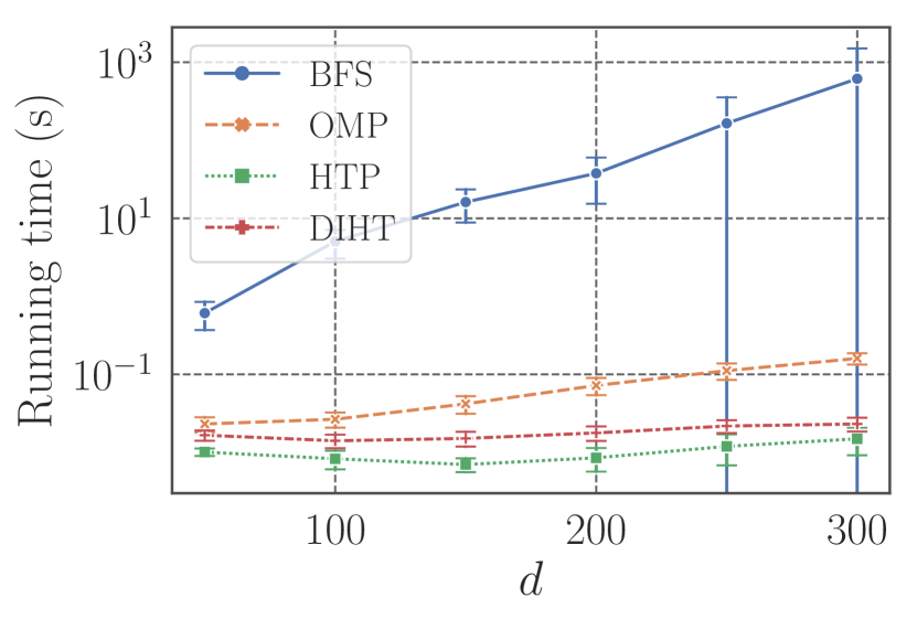
(a) Huber, Running Time

(b) Huber, Solver Call

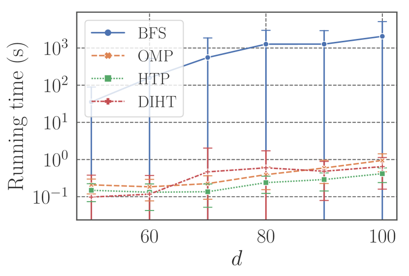
(c) Logistic, Running Time

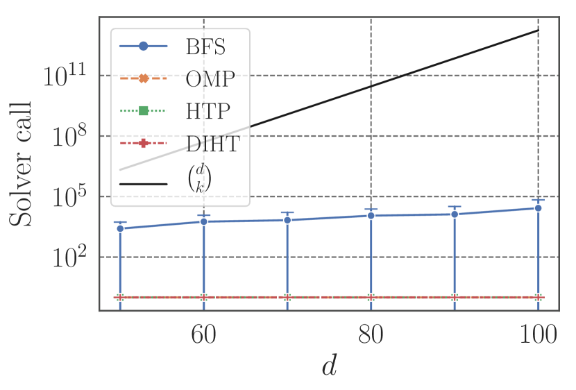
(d) Logistic, Solver Call

Figure 2: Running Times and Solver Calls. $\binom{d}{k}$ corresponds to the solver call of exhaustive search.

4.1.1 Computation Cost

We created $100$ random Huber and logistic instances with $d=50,100,\dots,300$ and $d=50,60,\dots,100$, respectively. We let $k=0.1k$ and $n=\lfloor 10k\log d\rfloor$. Figure 2 shows the running time and solver call, which indicates the number of times ${\tt SubtreeSolver}$ is executed, of each method. The solver calls of the inexact methods are regarded as $1$. Each curve and error bar indicate the mean and standard deviation calculated over $100$ instances. For comparison, we present the $\binom{d}{k}$ values, which correspond to the solver calls of a naive exhaustive search that solves problem (18) $\binom{d}{k}$ times. We see that BFS is far more efficient than the exhaustive search, which is too expensive to be used in practice. Note that the size of the state-space tree, $|V|$, is at least $\binom{d}{k}$; hence the results of solver calls confirm that BFS examines only a very small fraction of the tree. Furthermore, although BFS is slower than the inexact methods on average, BFS can sometimes run very fast as indicated by the error bars. We also counted the number of solved instances for each method: While BFS solved all the $600$ Huber instances and $600$ logistic instances, OMP, HTP, and DIHT solved 598, 172, and 233 Huber instance, respectively, and 464, 7, and 82 logistic instances, respectively. Note that these results regarding the inexact methods are obtained thanks to BFS, which always provides optimal solutions and enables us to see whether solutions obtained with inexact methods are optimal or not.

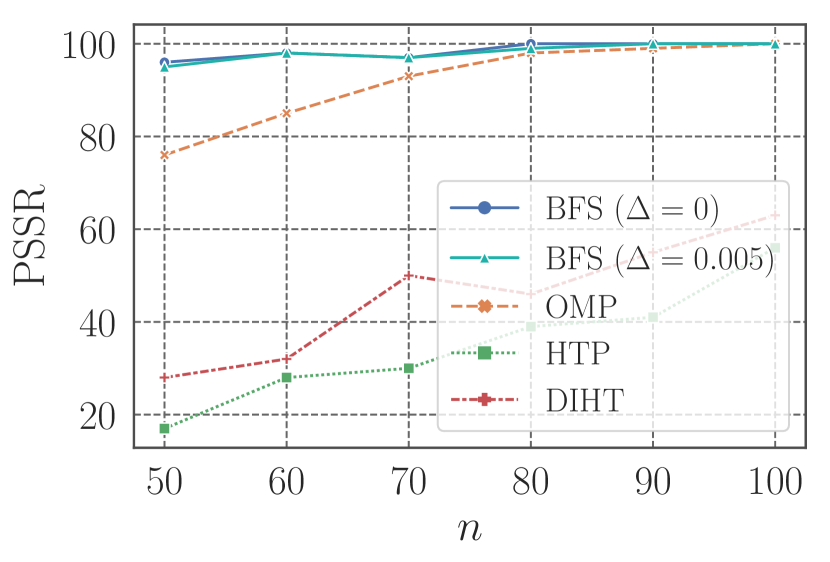
(a) Huber, PSSR

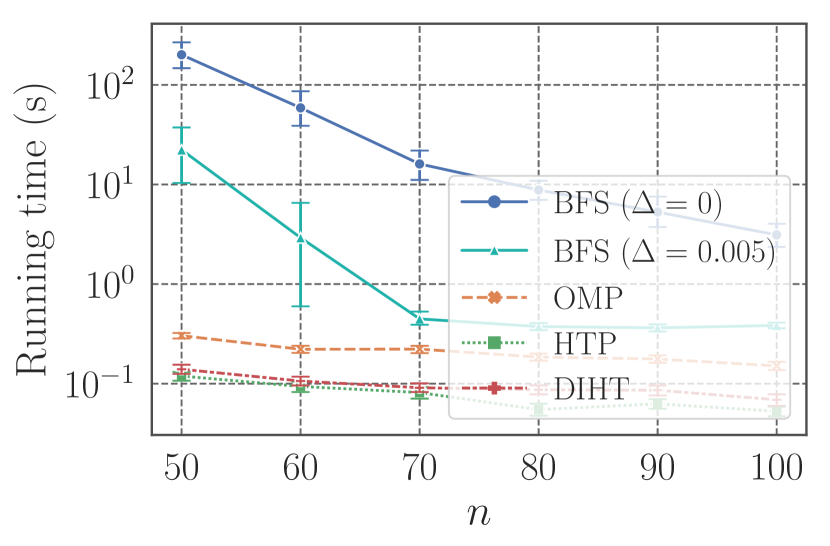
(b) Huber, Running Time

(c) Logistic, PSSR

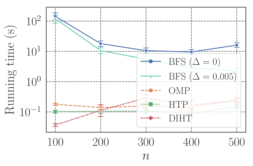
(d) Logistic, Running Time

Figure 3: PSSR and Running Times.

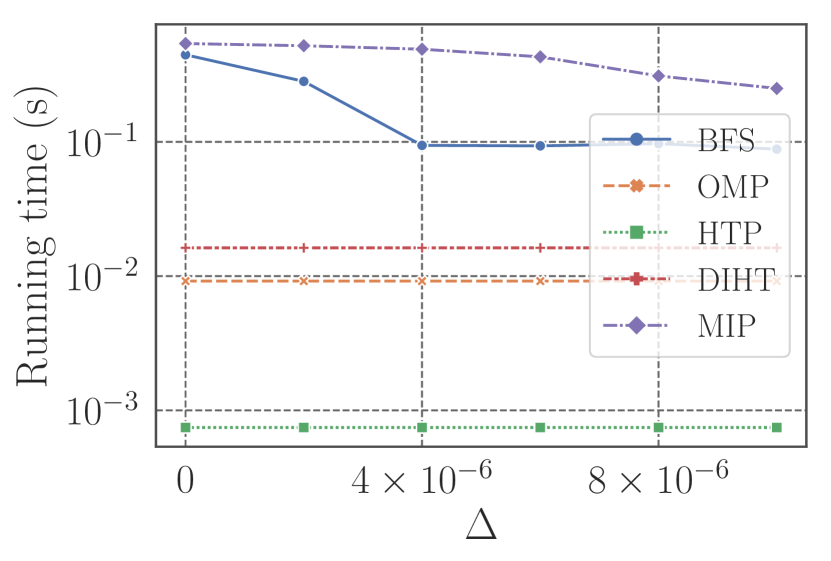
(a) Diabetes, Running Time

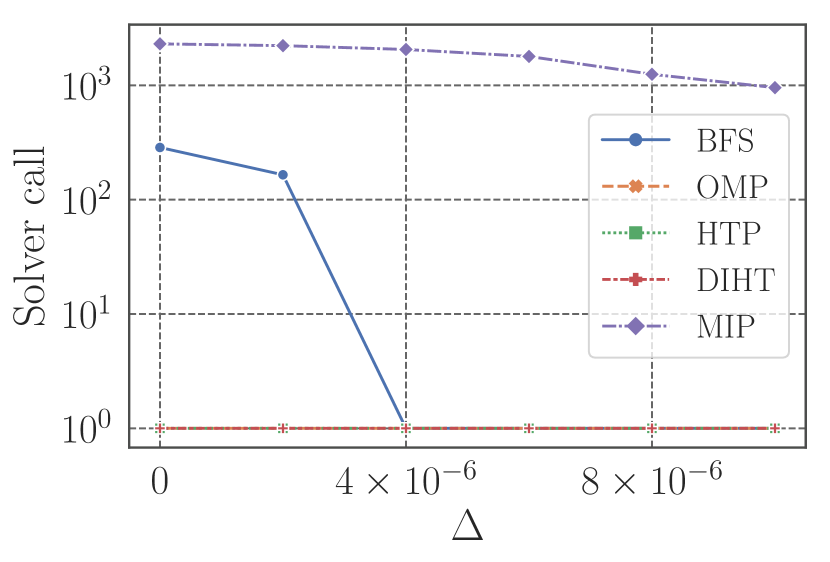
(b) Diabetes, Solver Call

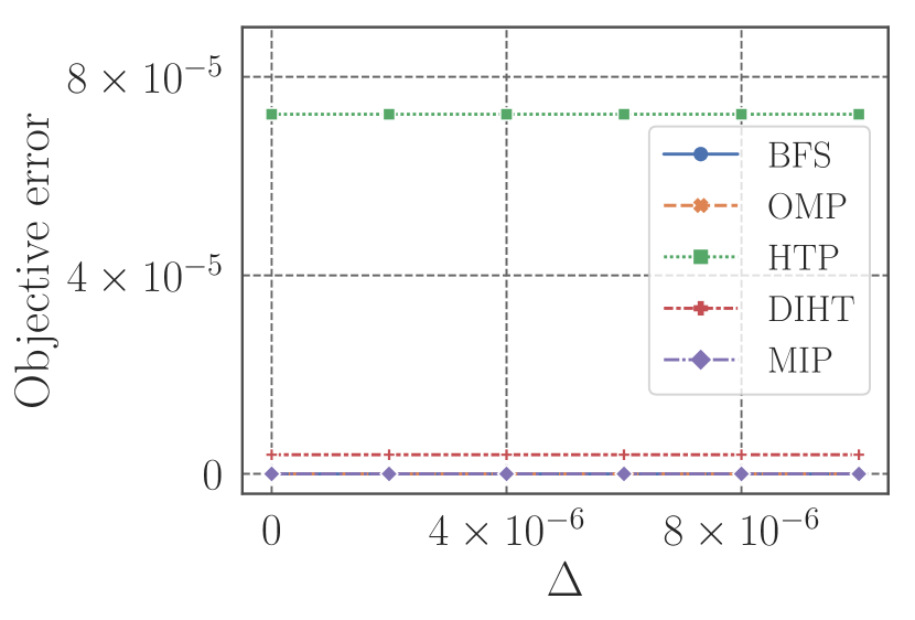
(c) Diabetes, Objective Error

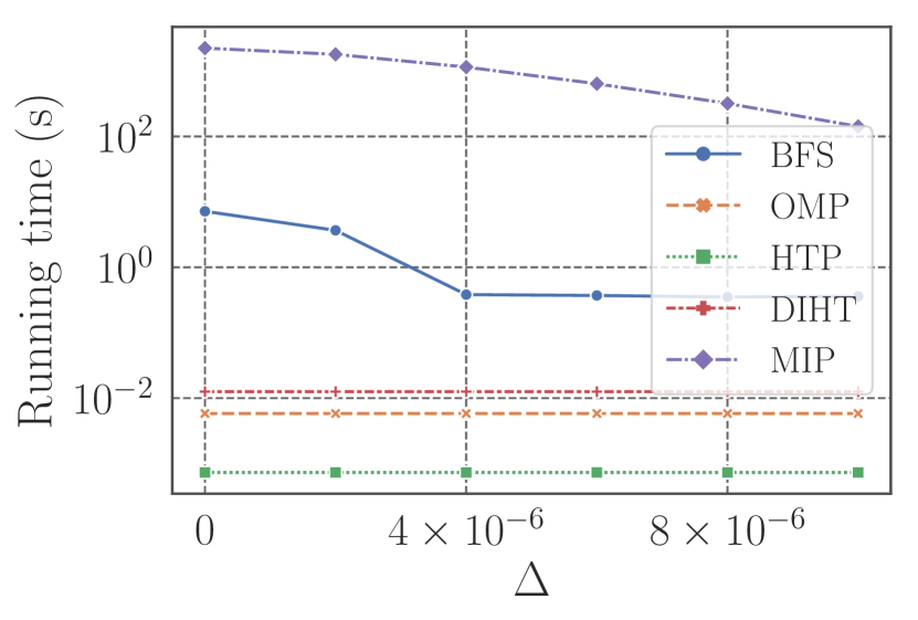
(d) Boston, Running Time

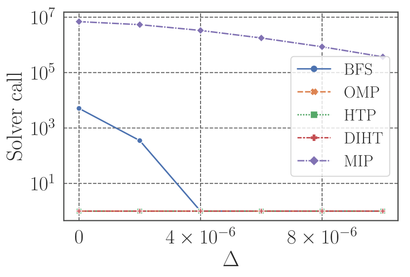
(e) Boston, Solver Call

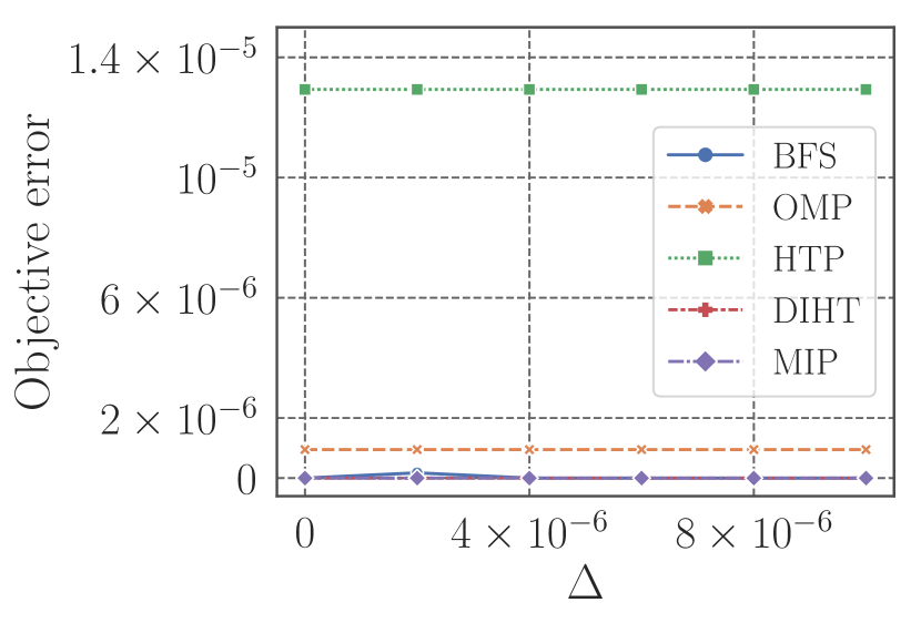
(f) Boston, Objective Error

Figure 4: Running Times, Solver Calls, and Objective Errors. Upper and lower figures show those of the Diabetes and Boston instances, respectively. We provide the results of OMP, HTP, and DIHT for comparison.

4.1.2 Support Recovery

We used Huber and logistic instances with $(d,k)=(50,5)$. We randomly generated $100$ Huber instances with $n=50,60,\dots,100$ and $100$ logistic instances with $n=100,200,\dots,500$. We applied the algorithms used in the above section and BFS that accepts $\Delta=0.005$ objective errors to the instances. We evaluated them with the percentage of successful support recovery (PSSR) as in (Liu et al., 2017), which counts the number of instances such that output solution $x$ satisfies $\mathop{\mathrm{supp}}\limits(x)=\mathop{\mathrm{supp}}\limits(x^{*})$ among the $100$ instances. We also measured running times of the algorithms. Figure 3 summarizes the results. BFS achieved higher PSSR performances than the inexact methods with both Huber and logistic instances. In particular, the performance gaps in Huber instances with small $n$ are significant as in Figure 3. Namely, to exactly solve NSM can be beneficial in terms of support recovery when only small samples are available. On the other hand, BFS tends to get faster as $n$ increases. This is because the condition of NSM instances typically becomes better as $n$ increases, which often makes the gap between $F(S)$ and ${\tt Low}_{S}$ smaller; i.e., ${\tt Low}_{S}$ can accurately estimate $F(S)$, and so BFS terminates quickly. To conclude, given moderate-size NSM instances whose true supports can hardly be recovered with inexact methods, BFS can be useful for recovering them at the expense of computation time. In Appendix D, we see that, given NSM instances with stronger regularization, BFS becomes faster while the PSSR performance deteriorates.

4.2 Real-world Instances

We compare BFS and MIP by using NSM instances with quadratic objectives, $P(x)=L_{\text{quadratic}}(Ax)+\frac{1}{2}\|\lambda\|^{2}$. The vector $b\in\mathbb{R}^{n}$ and matrix $A\in\mathbb{R}^{n\times d}$ were obtained from two scikit-learn datasets: Diabetes and Boston house-price, which for simplicity we call Boston. We normalized $b$ and each column of $A$ so that their $\ell_{2}$-norm became $1$. As in (Efron et al., 2004; Bertsimas et al., 2016), we considered the interaction and square effects of the original columns of $A$; any square effect whose original column had identical non-zeros was removed since they are redundant. Consequently, we obtained $A\in\mathbb{R}^{n\times d}$ with $(n,d)=(442,65)$ and $(506,103)$ for the Diabetes and Boston datasets, respectively. We let $\lambda=0.001$ and $k=10$. We applied BFS and MIP that accept various values of objective errors: $\Delta=0,2.0\times 10^{-6},4.0\times 10^{-6},\dots,1.0\times 10^{-5}$. The $\Delta$ value of MIP was controlled with the Gurobi parameter, MIPGapAbs. For comparison, we also applied the inexact methods to the instances, whose behavior is independent of $\Delta$ values. We evaluated the methods in terms of running times, solver calls, and objective errors, which are defined by $P(x)-P(x^{*})$ with output solution $x$. The solver call of MIP is the number of nodes explored by Gurobi.

Figure 4 summarizes the results. Both BFS and MIP become faster as $\Delta$ increases, and BFS is faster than MIP with every $\Delta$ value; in Boston instance with $\Delta=0$, BFS is more than $300$ times faster than MIP. Comparing the results with the two datasets ($d=65$ and $103$), we see that BFS is more scalable to large instances than MIP. For $\Delta\geq 4\times 10^{-6}$, BFS invoked ${\tt SubtreeSolver}$ only once. Namely, BFS detected that the solutions obtained by a single invocation of ${\tt SubtreeSolver}$ were guaranteed to have at most $\Delta$ errors without examining the descendant nodes. In contrast, MIP examined more nodes to obtain the $\Delta$-error guarantees, resulting in longer running times than those of BFS. This result is consistent with what we mentioned in Section 1.1. We see that BFS found optimal solutions except for the case of Boston instance with $\Delta=2\times 10^{-6}$, while none of the inexact methods succeeded in exactly solving both instances. We remark that the objective error of BFS does not always increase with $\Delta$ since the priority value, ${\tt Low}_{S}$, is not completely correlated with $F(S)$; i.e., a better solution can be obtained earlier.

5 CONCLUSION

We proposed a BFS algorithm for NSM with $\ell_{2}$-regularized convex objective functions. Experiments confirmed that our BFS existing exact methods are inapplicable, and that BFS can run faster than MIP with the latest commercial solver, Gurobi 8.1.0.

Appendix

Appendix A Computing Proximal Operator in Algorithm 3

We first introduce Moreau’s identity:

$$x=\alpha\mathop{\mathrm{prox}}\nolimits_{\alpha^{-1}f}(\alpha^{-1}x)+\mathop{\mathrm{prox}}\nolimits_{\alpha f^{*}}(x)$$

for any $\alpha>0$, $x\in\mathbb{R}^{m}$, and (proper closed) convex function $f:\mathbb{R}^{m}\to\mathbb{R}$. With this equality, the computation of $\mathop{\mathrm{prox}}\nolimits_{\tau_{t-1}L^{*}}(\beta^{t-1}-\tau_{t-1}Ay^{t-1})$ in Step 5 of Algorithm 3 can be reduced to the computation of the proximal operator for convex loss function $L(\cdot)$, which can be performed efficiently with various $L(\cdot)$.

We next see how to compute $\mathop{\mathrm{prox}}\nolimits_{\rho_{t}\tau_{t}(\frac{1}{2\lambda}\|\cdot\|^{2}_{k-s,2})^{*}}(\bar{y}^{t}_{S_{>}})$ in Step 12. Thanks to Moreau’s identity, it can be written as

$$\bar{y}^{t}_{S_{>}}-\rho_{t}\tau_{t}\mathop{\mathrm{prox}}\nolimits_{\frac{1}{2\lambda\rho_{t}\tau_{t}}\|\cdot\|^{2}_{k-s,2}}\left(\frac{1}{\rho_{t}\tau_{t}}\bar{y}^{t}_{S_{>}}\right).$$

Therefore, if we can compute the proximal operator for the top-$(k-s)$ $\ell_{2}$-norm, then we can perform Step 12. Below we show that it can be computed in $O(d)$ time.

Proximal-operator Computation for the Top-$k$ $\ell_{2}$-norm.

Given any positive integer $k$, $d$ ($k\leq d$), vector $v\in\mathbb{R}^{d}$, and parameter $\mu>0$, we show how to efficiently compute

$$\mathop{\mathrm{prox}}\nolimits_{\frac{\mu}{2}\|{\cdot}\|_{{k},2}^{2}}(v) =\mathop{\mathrm{argmin}}\limits_{x\in\mathbb{R}^{d}}\left\{\frac{\mu}{2}\|{x}\|_{{k},2}^{2}+\frac{1}{2}\|x-v\|^{2}\right\}$$ (21)

$$=\mathop{\mathrm{argmin}}\limits_{x\in\mathbb{R}^{d}}\left\{\mu\|{x}\|_{{k},2}^{2}+\|x-v\|^{2}\right\}.$$ (22)

Let $\mathop{\mathrm{sign}}\nolimits(v)\in\{-1,1\}^{d}$ denote a vector whose $i$th entry is $1$ if $v_{i}\geq 0$ and $-1$ otherwise. We have $\mathop{\mathrm{sign}}\nolimits(v)\odot v=(|v_{1}|,\dots,|v_{d}|)^{\top}\eqqcolon|v|$, where $\odot$ is the Hadamard (element-wise) product. We define $\sigma_{|v|}:{[d]}\to{[d]}$ as a permutation that rearranges the entries of $|v|$ in a non-increasing order. We abuse the notation and take $\sigma_{|v|}(x)\in\mathbb{R}^{d}$ to be a permutated vector for any given $x\in\mathbb{R}^{d}$; note that $\sigma_{|v|}(|v|)$ is non-increasing. We also define $\sigma_{|v|}^{-1}$ as the inverse permutation that satisfies $x=\sigma_{|v|}^{-1}(\sigma_{|v|}(x))$ for any $x\in\mathbb{R}^{d}$. Let $u\coloneqq\sigma_{|v|}(|v|)$ , which is non-negative and non-increasing. Note that, once we obtain

$$\tilde{x}\coloneqq\mathop{\mathrm{argmin}}\limits_{x\in\mathbb{R}^{d}}\left\{\mu\|{x}\|_{{k},2}^{2}+\|x-u\|^{2}\right\},$$ (23)

then the desired solution, $\mathop{\mathrm{prox}}\nolimits_{\frac{\mu}{2}\|{\cdot}\|_{{k},2}^{2}}(v)$, can be computed as $\mathop{\mathrm{sign}}\nolimits(v)\odot\sigma_{|v|}^{-1}(\tilde{x})$. Therefore, below we discuss how to compute $\tilde{x}$.

We define $f(x)\coloneqq\mu\|{x}\|_{{k},2}+\|x-u\|^{2}$. Since $u_{1}\geq\dots\geq u_{d}\geq 0$, we have $\tilde{x}_{1}\geq\dots\geq\tilde{x}_{d}\geq 0$; otherwise $\tilde{x}$ is not a minimizer. We let ${j_{{\tt start}}}\in[k]$ and ${j_{{\tt end}}}\in\{k,\dots,d\}$ be the smallest and largest indices such that $\tilde{x}_{j_{{\tt start}}}=\tilde{x}_{j_{{\tt end}}}=\tilde{x}_{k}$; i.e., it holds that

$$\tilde{x}_{1}\geq\dots>\tilde{x}_{j_{{\tt start}}}=\dots=\tilde{x}_{k}=\dots=\tilde{x}_{j_{{\tt end}}}>\dots\geq\tilde{x}_{d}.$$

We define ${\bar{u}}_{i}\coloneqq\frac{u_{i}}{1+\mu}$ for $i\in[k]$. If ${j_{{\tt start}}}={j_{{\tt end}}}=k$, we can readily obtain

$$\tilde{x}_{i}=\begin{cases}{\bar{u}}_{i}&\text{for $i=1,\dots,k$},\\ u_{i}&\text{for $i=k+1,\dots,d$}.\end{cases}$$ (24)

Note that this case occurs iff ${\bar{u}}_{k}\geq u_{k+1}$; in this case, $\tilde{x}$ can be obtained as above. We then consider the case ${j_{{\tt start}}}<{j_{{\tt end}}}$. Since $f$ is convex and $\tilde{x}$ is a minimizer, we have $0\in\partial f(\tilde{x})$, which implies

$$\tilde{x}_{i}=\begin{cases}{\bar{u}}_{i}&\text{for $i=1,\dots,{j_{{\tt start}}}-1$},\\ u_{i}&\text{for $i={j_{{\tt end}}}+1,\dots,d$}.\end{cases}$$ (25)

Namely, $\tilde{x}_{1},\dots,\tilde{x}_{{j_{{\tt start}}}-1}$ and $\tilde{x}_{{j_{{\tt end}}}+1},\dots,\tilde{x}_{d}$ can readily be obtained. Below we discuss how to compute ${j_{{\tt start}}}$, ${j_{{\tt end}}}$, and $\xi\coloneqq\tilde{x}_{j_{{\tt start}}}=\dots=\tilde{x}_{j_{{\tt end}}}$. Since $\tilde{x}$ is a minimizer of $f$, our aim is to find an optimal triplet, $({j_{{\tt start}}},{j_{{\tt end}}},\xi)\in[k]\times\{k,\dots,d\}\times\mathbb{R}$, that satisfies

$$\xi\in[u_{{j_{{\tt end}}}+1},{\bar{u}}_{{j_{{\tt start}}}-1}]$$ (26)

and minimizes

$$g({j_{{\tt start}}},{j_{{\tt end}}},\xi)\coloneqq{}(1+\mu)\sum_{i={j_{{\tt start}}}}^{k}(\xi-{\bar{u}}_{i})^{2}+\sum_{i=k+1}^{{j_{{\tt end}}}}(\xi-u_{i})^{2},$$ (27)

where we regard ${\bar{u}}_{0}=+\infty$ and $u_{d+1}=0$, and we take the second term on the RHS to be $0$ if ${j_{{\tt end}}}=k$. Note that, once $({j_{{\tt start}}},{j_{{\tt end}}})$ is fixed, computing optimal $\xi$ reduces to a one-dimensional quadratic minimization problem with constraint (26), whose solution $\xi$ can be written as follows:

$$\xi=\min\{{\bar{u}}_{{j_{{\tt start}}}-1},\max\{u_{{j_{{\tt end}}}+1},\tilde{\xi}\}\},$$ (28)

where

$$\tilde{\xi}=\frac{\sum_{i={j_{{\tt start}}}}^{{j_{{\tt end}}}}u_{i}}{\mu(k-{j_{{\tt start}}}+1)+{j_{{\tt end}}}-{j_{{\tt start}}}+1}.$$

In what follows, we discuss how to find $({j_{{\tt start}}},{j_{{\tt end}}})$ that constitutes an optimal triplet.

We first show that triplet $({j_{{\tt start}}},{j_{{\tt end}}},\xi)$ that satisfies (26) is sub-optimal if $\xi<{\bar{u}}_{j_{{\tt start}}}$ holds. In this case, we have

$$g({j_{{\tt start}}}+1,{j_{{\tt end}}},\xi)\leq g({j_{{\tt start}}},{j_{{\tt end}}},\xi)$$

and triple $({j_{{\tt start}}}+1,{j_{{\tt end}}},\xi)$ satisfies constraint (26), i.e.,

$$\xi\in[u_{{j_{{\tt end}}}+1},{\bar{u}}_{{j_{{\tt start}}}}],$$

since $\xi<{\bar{u}}_{{j_{{\tt start}}}}$. Namely, $({j_{{\tt start}}}+1,{j_{{\tt end}}},\xi)$ is feasible and achieves at least as small $g$ value as $({j_{{\tt start}}},{j_{{\tt end}}},\xi)$. Below we focus on the case where ${\bar{u}}_{j_{{\tt start}}}\leq\xi$ holds.

Algorithm 4 Computation of $\mathop{\mathrm{prox}}\nolimits_{\frac{\mu}{2}\|{\cdot}\|_{{k},2}^{2}}(v)$

1:$u\leftarrow\sigma_{|v|}(|v|)$

2:${\bar{u}}_{i}\leftarrow u_{i}/(1+\mu)$ for $i\in[k]$

3:if ${\bar{u}}_{k}\geq u_{k+1}$ then

4:     $\tilde{x}\leftarrow({\bar{u}}_{1},\dots,{\bar{u}}_{k},u_{k+1},\dots,u_{d})^{\top}$

5:     return $\mathop{\mathrm{sign}}\nolimits(v)\odot\sigma_{|v|}^{-1}(\tilde{x})$

6:${\hat{j}}\leftarrow k$, $g_{\min}\leftarrow+\infty$, and ${\tt Examined}\leftarrow\emptyset$

7:for ${j_{{\tt start}}}=1,\dots,k$ do

8:     ${\tt Endpoints}\leftarrow\{j\in[d]\mathrel{|}u_{j}>{\bar{u}}_{j_{{\tt start}}}\ \text{and}\ j\geq{\hat{j}}\}$

9:     for ${j_{{\tt end}}}\in{\tt Endpoints}$ do

10:         $\tilde{\xi}\leftarrow\frac{\sum_{i={j_{{\tt start}}}}^{{j_{{\tt end}}}}u_{i}}{\mu(k-{j_{{\tt start}}}+1)+{j_{{\tt end}}}-{j_{{\tt start}}}+1}$

11:         $\xi\leftarrow\min\{{\bar{u}}_{{j_{{\tt start}}}-1},\max\{u_{{j_{{\tt end}}}+1},\tilde{\xi}\}\}$

12:         if $g({j_{{\tt start}}},{j_{{\tt end}}},\xi)<g_{\min}$ then

13:              $({j^{*}_{{\tt start}}},{j^{*}_{{\tt end}}},\xi^{*})\leftarrow({j_{{\tt start}}},{j_{{\tt end}}},\xi)$

14:              ${g_{\min}}\leftarrow g({j^{*}_{{\tt start}}},{j^{*}_{{\tt end}}},\xi^{*})$               

15:     ${\tt Examined}\leftarrow{\tt Examined}\cup{\tt Endpoints}$

16:     if ${\tt Examined}\neq\emptyset$ then

17:         ${\hat{j}}\leftarrow\max{\tt Examined}$      

18:$\tilde{x}\leftarrow({\bar{u}}_{1},\dots,{\bar{u}}_{{j^{*}_{{\tt start}}}-1},\xi^{*},\dots,\xi^{*},u_{{j^{*}_{{\tt end}}}+1},\dots,u_{d})^{\top}$

19:return $\mathop{\mathrm{sign}}\nolimits(v)\odot\sigma_{|v|}^{-1}(\tilde{x})$

We then prove that triple $({j_{{\tt start}}},{j_{{\tt end}}},\xi)$ satisfying (26) and ${\bar{u}}_{{j_{{\tt start}}}}\geq u_{{j_{{\tt end}}}}$ is sub-optimal. In this case, we have

$$g({j_{{\tt start}}},{j_{{\tt end}}}-1,\xi)\leq g({j_{{\tt start}}},{j_{{\tt end}}},\xi)$$

and triple $({j_{{\tt start}}},{j_{{\tt end}}}-1,\xi)$ satisfies constraint (26), i.e.,

$$\xi\in[u_{{j_{{\tt end}}}},{\bar{u}}_{{j_{{\tt start}}}-1}],$$

since $u_{j_{{\tt end}}}\leq{\bar{u}}_{{j_{{\tt start}}}}\leq\xi$. Namely, $({j_{{\tt start}}},{j_{{\tt end}}}-1,\xi)$ is feasible and achieves at least as small $g$ value as $({j_{{\tt start}}},{j_{{\tt end}}},\xi)$. Therefore, to find an optimal triplet, we only need to examine $({j_{{\tt start}}},{j_{{\tt end}}},\xi)$ that satisfies constraint (26) and

$$u_{j_{{\tt end}}}>{\bar{u}}_{{j_{{\tt start}}}}.$$ (29)

We fix ${j_{{\tt start}}}\in[k]$ and define

$${\hat{j}}\coloneqq\max\{j\in\{k,\dots,d\}\mathrel{|}u_{j}>{\bar{u}}_{{j_{{\tt start}}}-1}\}.$$

Then,

$${j_{{\tt end}}}\geq{\hat{j}}\quad\text{(i.e., $u_{j_{{\tt end}}}\leq u_{\hat{j}}$)}$$ (30)

must hold for the following reason: If ${j_{{\tt end}}}+1\leq{\hat{j}}$ holds, we have $u_{{j_{{\tt end}}}+1}\geq u_{{\hat{j}}}>{\bar{u}}_{{j_{{\tt start}}}-1}$, which means no $\xi$ satisfies constraint (26).

Taking (29) and (30) into account, once ${j_{{\tt start}}}\in[k]$ is fixed, endpoint ${j_{{\tt end}}}$ to be examined satisfies

$$u_{j_{{\tt end}}}>{\bar{u}}_{{j_{{\tt start}}}}\quad\text{and}\quad{j_{{\tt end}}}\geq{\hat{j}}=\max\{j\in\{k,\dots,d\}\mathrel{|}u_{j}>{\bar{u}}_{{j_{{\tt start}}}-1}\}.$$ (31)

Therefore, by examining ${j_{{\tt start}}}=1,\dots,k$ sequentially and maintaining ${\tt Examined}=\{j\in\{k,\dots,d\}\mathrel{|}u_{j}>{\bar{u}}_{j_{{\tt start}}}\}$ as in Algorithm 4, we can find an optimal triplet $({j^{*}_{{\tt start}}},{j^{*}_{{\tt end}}},\xi^{*})$, with which we can obtain $\mathop{\mathrm{prox}}\nolimits_{\frac{\mu}{2}\|{\cdot}\|_{{k},2}^{2}}$.

We examine the complexity of Algorithm 4. Let ${\tt Endpoints}_{i}$ be the list of endpoints constructed in the $i$th iteration for $i\in[k]$. Since ${\tt Endpoints}_{i}$ and ${\tt Endpoints}_{i+1}$ have at most one common element and $\bigcup_{i\in[k]}{\tt Endpoints}_{i}$ includes at most $d-k+1$ elements, we have $\sum_{i=1}^{k}|{\tt Endpoints}_{i}|\leq d-k+1+(k-1)=d$. Namely, Algorithm 4 examines at most $d$ candidate triplets, hence Algorithm 4 runs in $O(d)$ time.

Algorithm 5 SGA for computing ${\tt Low}_{S}$ and ${\tt Sol}_{S}$

1:Initialize $\beta^{0}$ and $\eta_{0}$.

2:Fix $\epsilon>0$. $\triangleright$ $\epsilon=10^{-5}$ in the experiments

3:for $t=1,2,\dots$ do

4:     Compute a supergradient $g^{t-1}\in\partial D(\beta^{t-1};S)$.

5:     $\eta_{t}\leftarrow 2\times\eta_{t-1}$

6:     loop$\triangleright$ Backtracking of step-size $\eta_{t}$

7:         $\beta^{t}\leftarrow\mathcal{P}_{\mathcal{F}}(\beta^{t-1}+\eta_{t}g^{t-1})$

8:         if $D(\beta^{t};S)\geq D(\beta^{t-1};S)$ then

9:              break          

10:         $\eta_{t}\leftarrow 0.5\times\eta_{t}$      

11:     if $(D(\beta^{t};S)-D(\beta^{t-1};S))/P_{\min}\leq\epsilon$ then

12:         

$x^{t}_{S}\leftarrow-\frac{1}{\lambda}A_{S}^{\top}\beta^{t}$,  $x^{t}_{S_{\leq}\setminus S}\leftarrow 0$,  and

$x^{t}_{S_{>}}\leftarrow-\frac{1}{\lambda}\mathcal{T}_{k-s}(A_{S_{>}}^{\top}\beta^{t})$

13:         ${\tt Low}_{S}\leftarrow D(\beta^{t};S)$

14:         ${\tt Sol}_{S}\leftarrow\mathop{\mathrm{argmin}}\limits_{\mathop{\mathrm{supp}}\limits(x)\subseteq\mathop{\mathrm{supp}}\limits(x^{t})}P(x)$

15:         return ${\tt Low}_{S}$, ${\tt Sol}_{S}$      

Appendix B Comparison of Supergradient Ascent and Primal-dual Algorithm with Linesearch

As mentioned in Section 3.1, we can use the supergradient ascent (SGA) for solving

$$\operatorname*{maximize}_{\beta\in\mathbb{R}^{n}}\quad D(\beta;S)$$ (32)

instead of PDAL. We first describe the details of SGA based on (Liu et al., 2017), and then we experimentally compare two BFS algorithms that use SGA and PDAL as their subroutines.

B.1 Details of SGA

Let ${\mathcal{F}}\coloneqq\{\beta\in\mathbb{R}^{n}\mathrel{|}D(\beta;S)>-\infty\}$ be the effective domain of $D(\beta;S)$ and $\mathcal{P}_{\mathcal{F}}(\cdot)$ be the Euclidean projection operator onto ${\mathcal{F}}$. If $\partial L^{*}(\beta)\subseteq\mathbb{R}^{n}$ is the super-differential of $L^{*}(\beta)$, the super-differential of $D(\beta;S)$ is given by

$$\partial D(\beta;S)=\{A\tilde{x}(\beta;S)-\tilde{g}\mathrel{|}\tilde{g}\in\partial L^{*}(\beta)\}.$$

With these definitions, the SGA procedure for computing ${\tt Low}_{S}$ and ${\tt Sol}_{S}$ can be described as in Algorithm 5. We can use the warm-start and pruning techniques as in Section 3.2, but the details of the warm-start technique for initializing $\beta^{0}$ and $\eta_{0}$ are slightly different from those of PDAL as explained below. When executing SGA with $S=\emptyset$ at the beginning of BFS, we set $\beta^{0}\leftarrow 0$ and $\eta_{0}\leftarrow 1$. We now suppose that ${S^{\prime}}\in V$ is popped from $\mathrm{MinHeap}$ and that we are about to compute ${\tt Low}_{S}$ and ${\tt Sol}_{S}$, where $({S^{\prime}},S)\in E$. Let $\beta_{S^{\prime}}$ be a dual solution obtained in the last iteration of SGA executed for ${S^{\prime}}$; i.e., ${\tt Low}_{{S^{\prime}}}=D(\beta_{S^{\prime}};{S^{\prime}})$. When executing SGA to maximize $D(\beta;S)$, we let $\beta^{0}\leftarrow\beta_{S^{\prime}}$. Furthermore, we set $\eta^{0}\leftarrow\eta_{S^{\prime}}$, where $\eta_{S^{\prime}}$ is a step-size used to obtain $\beta^{1}$ in SGA executed for ${S^{\prime}}$.

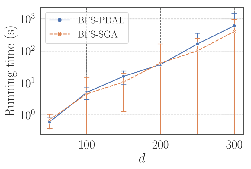
(a) Running Time

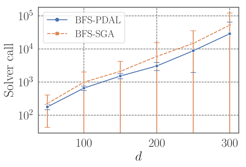
(b) Solver Call

Figure 5: Running Times and Solver Calls of BFS-SGA and BFS-PDAL.

B.2 Experimental Comparison

We experimentally compare two BFS algorithms with SGA and PDAL, which we call BFS-SGA and BFS-PDAL, respectively. The experimental setting used here is the same as the Huber instance in Section 4.1.1. We observed the running times and solver calls of BFS-SGA and BFS-PDAL. As with BFS-PDAL, BFS-SGA used warm-start and pruning techniques.

Figure 5 shows the results, where each curve and error bar indicate the mean and standard deviation calculated over $100$ random instances. While the running times of the two methods are almost the same, BFS-PDAL is more efficient in terms of solver calls. This result implies that ${\tt Low}_{S}$ values computed by PDAL and SGA are different even though $D(\beta;S)$ is concave; in fact, due to the non-smoothness of $D(\beta;S)$, SGA sometimes fails to maximize $D(\beta;S)$. As a result, BFS-SGA tends to require more solver calls than BFS-PDAL on average. Note that, while the computation costs of SGA and PDAL are polynomial in $d$, the number of solver calls can increase exponentially in $k$; i.e., it is more important to reduce the number of solver calls than to reduce the running time of subroutines (SGA and PDAL). To conclude, BFS-PDAL is expected to be more scalable to larger instances than BFS-SGA, which motivates us to employ PDAL.

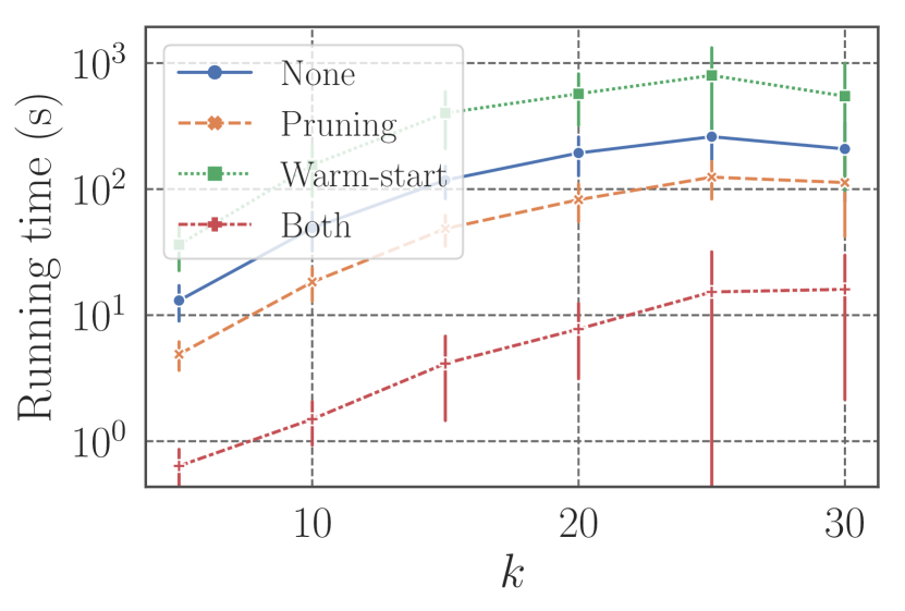
(a) Running Time

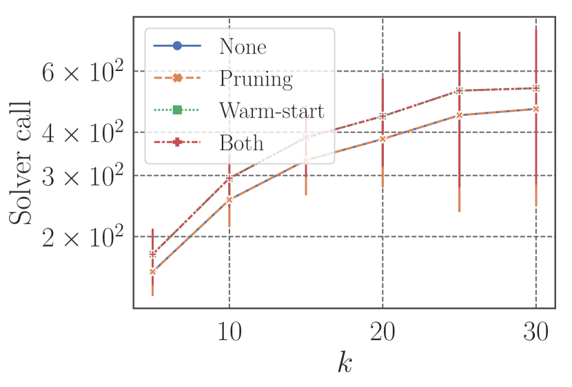
(b) Solver Call

Figure 6: Running Times and Solver Calls of BFS with and without Pruning and Warm-start Techniques.

Appendix C Ablation Study

We experimentally study the degree to which the pruning and warm-start techniques speed up BFS. We used the Huber instances (Section 4.1) with $d=50$, $k=5,10,\dots,30$, and $n=\left\lfloor{10k\log d}\right\rfloor$; for each $k$ value we generated $100$ random instances.

Figure 6 presents running times and solver calls. Each value and error bar are mean and standard deviation calculated over $100$ instances. We see that the warm-start technique alone does not always accelerate BFS, but the combination of pruning and warm-start greatly reduces the running time. This is because, if a good solution is available thanks to warm-start at the beginning of ${\tt SubtreeSolver}$, then it can be force-quitted quickly via the pruning procedure. We also see that, while the size of the state-space tree increases exponentially in $k$, the running time and solver call grow sub-linearly in $k$ in the semi-log plots, which implies that the search space is effectively reduced thanks to our prioritization method with ${\tt SubtreeSolver}$.

Appendix D Additional Experimental Results

We examine how the PSSR performances and running times change with stronger regularization. The experimental settings used here are almost the same as those of Section 4.1.2. The only difference is the $\lambda$ value: We let $\lambda=0.01$ and $0.002$ for Huber and logistic instances, respectively.

Figure 7 presents the PSSR values and running times. Relative to the results shown in Section 4.1.2, BFS became faster and the PSSR performance gap between BFS and the inexact methods became smaller. The reason for this result is as follows: When strongly regularized, objective functions become convex more strongly. This typically reduces the gap, $F(S)-{\tt Low}_{S}$, and so BFS terminates more quickly. Furthermore, it becomes easier to solve NSM instances exactly with inexact methods. Namely, it tends to be easy to exactly solve NSM instances with strong regularization. On the other hand, due to the over regularization, optimal solutions to such NSM instances often fail to recover the true support, hence the PSSR performance of BFS deteriorates; consequently, the gap between BFS and inexact methods became smaller. To conclude, if we are to achieve high support recovery performance, we need to solve NSM instances with moderate regularization, which is often hard for inexact methods as implied by the experimental results in Section 4.1.2. This observation emphasizes the utility of our BFS, which is empirically efficient enough for exactly solving moderate-size NSM instances.

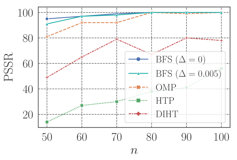
(a) Huber, PSSR

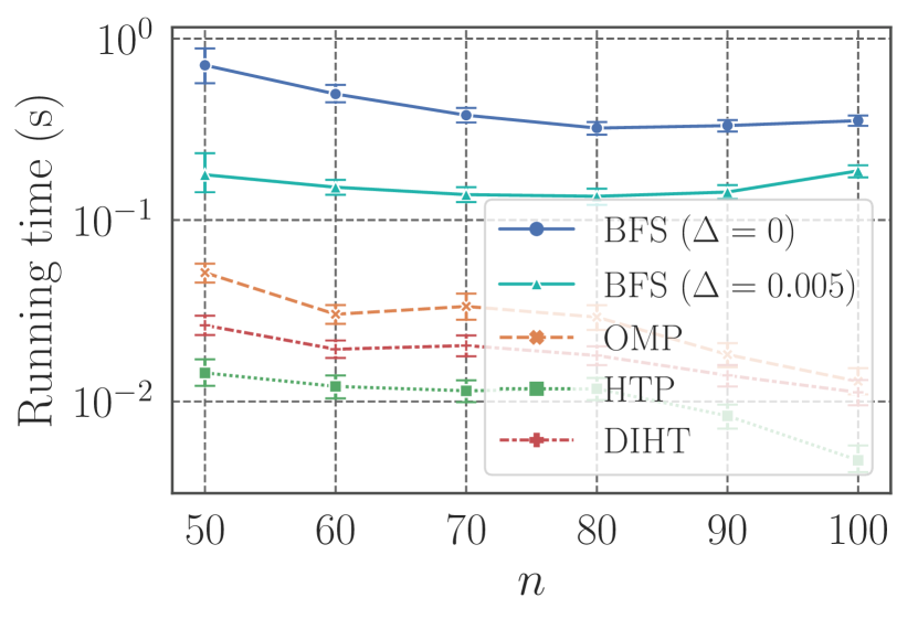
(b) Huber, Running Time

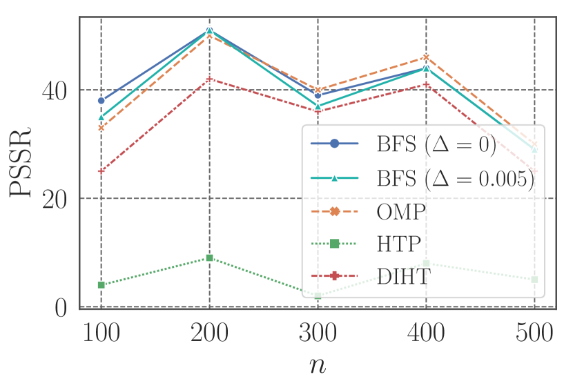
(c) Logistic, PSSR

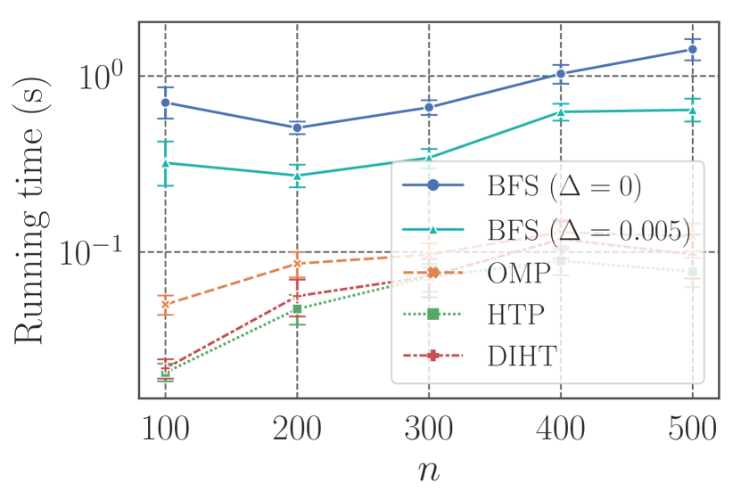
(d) Logistic, Running Time

Figure 7: PSSR and Running Times.

References

- Arai et al. (2015) H. Arai, C. Maung, and H. Schweitzer. Optimal column subset selection by A-star search. In Proceedings of the 29th AAAI Conference on Artificial Intelligence. AAAI Press, 2015.
- Avis and Fukuda (1996) D. Avis and K. Fukuda. Reverse search for enumeration. Discrete Appl. Math., 65(1):21 – 46, 1996.
- Bertsimas and Van Parys (2017) D. Bertsimas and B. Van Parys. Sparse high-dimensional regression: Exact scalable algorithms and phase transitions. arXiv preprint arXiv:1709.10029, 2017.
- Bertsimas et al. (2016) D. Bertsimas, A. King, and R. Mazumder. Best subset selection via a modern optimization lens. Ann. Statist., 44(2):813–852, 2016.
- Bhatia et al. (2017) K. Bhatia, P. Jain, P. Kamalaruban, and P. Kar. Consistent robust regression. In Advances in Neural Information Processing Systems 30, pages 2110–2119. Curran Associates, Inc., 2017.
- Blumensath and Davies (2009) T. Blumensath and M. E. Davies. Iterative hard thresholding for compressed sensing. Appl. Comput. Harmon. Anal., 27(3):265–274, 2009.
- Bourguignon et al. (2016) S. Bourguignon, J. Ninin, H. Carfantan, and M. Mongeau. Exact sparse approximation problems via mixed-integer programming: Formulations and computational performance. IEEE Trans. Signal Process., 64(6):1405–1419, 2016.
- Chen et al. (2015) W. Chen, Y. Chen, and K. Weinberger. Filtered search for submodular maximization with controllable approximation bounds. In Proceedings of the 18th International Conference on Artificial Intelligence and Statistics, volume 38, pages 156–164. PMLR, 2015.
- Dechter and Pearl (1985) R. Dechter and J. Pearl. Generalized best-first search strategies and the optimality of A*. J. ACM, 32(3):505–536, 1985.
- Defazio (2016) A. Defazio. A simple practical accelerated method for finite sums. In Advances in Neural Information Processing Systems 29, pages 676–684. Curran Associates, Inc., 2016.
- Ebendt and Drechsler (2009) R. Ebendt and R. Drechsler. Weighted search — unifying view and application. Artificial Intelligence, 173(14):1310 – 1342, 2009.
- Efron et al. (2004) B. Efron, T. Hastie, I. Johnstone, and R. Tibshirani. Least angle regression. Ann. Statist., 32(2):407–499, 2004.
- Elenberg et al. (2018) E. R. Elenberg, R. Khanna, A. G. Dimakis, and S. Negahban. Restricted strong convexity implies weak submodularity. Ann. Statist., 46(6B):3539–3568, 2018.
- Foucart (2011) S. Foucart. Hard thresholding pursuit: An algorithm for compressive sensing. SIAM J. Optim., 49(6):2543–2563, 2011.
- Hansen and Zhou (2007) E. A. Hansen and R. Zhou. Anytime heuristic search. J. Artif. Int. Res., 28(1):267–297, 2007.
- Hart et al. (1968) P. E. Hart, N. J. Nilsson, and B. Raphael. A formal basis for the heuristic determination of minimum cost paths. IEEE Trans. Syst. Sci. Cybernet., 4(2):100–107, 1968.
- Hocking and Leslie (1967) R. R. Hocking and R. N. Leslie. Selection of the best subset in regression analysis. Technometrics, 9(4):531–540, 1967.
- Huang et al. (2018) J. Huang, Y. Jiao, Y. Liu, and X. Lu. A constructive approach to penalized regression. J. Mach. Learn. Res., 19(1):403–439, 2018.
- Jain et al. (2014) P. Jain, A. Tewari, and P. Kar. On iterative hard thresholding methods for high-dimensional M-estimation. In Advances in Neural Information Processing Systems 27, pages 685–693. Curran Associates, Inc., 2014.
- Karahanoglu and Erdogan (2012) N. B. Karahanoglu and H. Erdogan. A* orthogonal matching pursuit: Best-first search for compressed sensing signal recovery. Digit. Signal Process., 22(4):555 – 568, 2012.
- Liu et al. (2017) B. Liu, X.-T. Yuan, L. Wang, Q. Liu, and D. N. Metaxas. Dual iterative hard thresholding: From non-convex sparse minimization to non-smooth concave maximization. In Proceedings of the 34th International Conference on Machine Learning, volume 70, pages 2179–2187. PMLR, 2017.
- Malitsky and Pock (2018) Y. Malitsky and T. Pock. A first-order primal-dual algorithm with linesearch. SIAM J. Optim., 28(1):411–432, 2018.
- Miyashiro and Takano (2015) R. Miyashiro and Y. Takano. Mixed integer second-order cone programming formulations for variable selection in linear regression. European J. Oper. Res., 247(3):721 – 731, 2015.
- Natarajan (1995) B. K. Natarajan. Sparse approximate solutions to linear systems. SIAM J. Optim., 24(2):227–234, 1995.
- Pati et al. (1993) Y. C. Pati, R. Rezaiifar, and P. S. Krishnaprasad. Orthogonal matching pursuit: recursive function approximation with applications to wavelet decomposition. In Proceedings of the 27th Asilomar Conference on Signals, Systems and Computers, pages 40–44 vol.1, 1993.
- Pearl (1984) J. Pearl. Heuristics: Intelligent Search Strategies for Computer Problem Solving. Addison-Wesley Longman Publishing Co., Inc., Boston, MA, USA, 1984.
- Sakaue and Ishihata (2018) S. Sakaue and M. Ishihata. Accelerated best-first search with upper-bound computation for submodular function maximization. In Proceedings of the 32nd AAAI Conference on Artificial Intelligence, 2018.
- Sato et al. (2016) T. Sato, Y. Takano, R. Miyashiro, and A. Yoshise. Feature subset selection for logistic regression via mixed integer optimization. Comput. Optim. Appl., 64(3):865–880, 2016.
- Shalev-Shwartz and Zhang (2016) S. Shalev-Shwartz and T. Zhang. Accelerated proximal stochastic dual coordinate ascent for regularized loss minimization. Math. Program., 155(1):105–145, 2016.
- Valenzano et al. (2013) R. Valenzano, S. J. Arfaee, J. Thayer, R. Stern, and N. R. Sturtevant. Using alternative suboptimality bounds in heuristic search. In Proceedings of the 23rd International Conference on Automated Planning and Scheduling, pages 233–241. AAAI Press, 2013.
- Yuan et al. (2014) X. Yuan, P. Li, and T. Zhang. Gradient hard thresholding pursuit for sparsity-constrained optimization. In Proceedings of the 31st International Conference on Machine Learning, volume 32, pages 127–135. PMLR, 2014.
- Yuan et al. (2016) X. Yuan, P. Li, and T. Zhang. Exact recovery of hard thresholding pursuit. In Advances in Neural Information Processing Systems 29, pages 3558–3566. Curran Associates, Inc., 2016.