Space–time reduced order model for large-scale linear dynamical systems with application to Boltzmann transport problems

Abstract

A classical reduced order model for dynamical problems involves spatial reduction of the problem size. However, temporal reduction accompanied by the spatial reduction can further reduce the problem size without losing accuracy much, which results in a considerably more speed-up than the spatial reduction only. Recently, a novel space–time reduced order model for dynamical problems has been developed [14], where the space–time reduced order model shows an order of a hundred speed-up with a relative error of $10^{-4}$ for small academic problems. However, in order for the method to be applicable to a large-scale problem, an efficient space–time reduced basis construction algorithm needs to be developed. We present incremental space–time reduced basis construction algorithm. The incremental algorithm is fully parallel and scalable. Additionally, the block structure in the space–time reduced basis is exploited, which enables the avoidance of constructing the reduced space–time basis. These novel techniques are applied to a large-scale particle transport simulation with million and billion degrees of freedom. The numerical example shows that the algorithm is scalable and practical. Also, it achieves a tremendous speed-up, maintaining a good accuracy. Finally, error bounds for space-only and space–time reduced order models are derived.

Keywords— Space–time reduced order model, incremental singular value decomposition, Boltzmann transport equations, linear dynamical systems, block structure, optimal projection, proper orthogonal decomposition

1 Introduction

Many computational models for physics simulations are formulated as linear dynamical systems. Examples of linear dynamical systems include the computational model for the signal propagation and interference in electric circuits, storm surge prediction models before an advancing hurricane, vibration analysis in large structures, thermal analysis in various media, neuro-transmission models in the nervous system, various computational models for micro-electro-mechanical systems, and various particle transport simulations. Depending on the complexity of geometries and desirable fidelity level, these problems become easily large-scale problems. For example, the Boltzmann Transport Equation (BTE) has seven independent variables, i.e., three spatial variables, two directional variables, one energy variable, and one time variable. It is not hard to see that the BTE can easily lead to a high dimensional discretized problem. Additionally, the complex geometry (e.g., reactors with thousands of pins and shields) can lead to a large-scale problem. As an example, a problem with 20 angular directions, a cubit spatial domain of 100 x 100 x 100 elements, 16 energy groups, and 100 time steps leads to 32 billion unknowns. The large-scale hinders a fast forward solve and prevents the multi-query setting problems, such as uncertainty quantification, design optimization, and parameter study, from being tractable. Therefore, developing a Reduced Order Model (ROM) that accelerates the solution process without losing much accuracy is essential.

There are several model order reduction approaches available for linear dynamical systems: (i) Balanced truncation [29, 28] in control theory community is the most famous one. It has explicit error bounds and guarantees stability. However, it requires the solution of two Lyapunov equations to construct bases, which is a formidable task in large-scale problems. (ii) The moment-matching methods [4, 19] provide a computationally efficient framework using Krylov subspace techniques in an iterative fashion where only matrix-vector multiplications are required. The optimal $H_{2}$ tangential interpolation for nonparametric systems [19] is also available. The most crucial part of the moment-matching methods is location of samples where moments are matched. Also, it is not a data-driven approach, meaning that no data is used to construct ROM. (iii) Proper Generalized Decomposition (PGD) [2] was first developed as a numerical method of solving boundary value problems, later extended to dynamical problems [3]. The main assumption of the method is a separated solution representation in space and time, which gives a way for an efficient solution procedure. Therefore, it is considered as a model reduction technique. However, PGD is not a data-driven approach.

Often there are many data available either from experiments or high-fidelity simulations. Those data contain valuable information about the system of interest. Therefore, data-driven methods can maximize the usage of the existing data and enable the construction of an optimal ROM. Dynamic Mode Decomposition (DMD) is a data-driven approach that generates reduced modes that embed an intrinsic temporal behavior. It was first developed by Peter Schmid in [34] and populated by many other scientists. For more detailed information about DMD, we refer to this preprint [37]. As another data-driven approach, Proper Orthogonal decomposition (POD) [6] gives the data-driven optimal basis through the method of snapshots. However, most of POD-based ROMs for linear dynamical systems apply spatial projection only. Temporal complexity is still proportional to temporal discretization of its high-fidelity model. In order to achieve an optimal reduction, a space–time ROM needs to be built where both spatial and temporal projections are applied. In literature, some space–time ROMs are available [14, 38, 41, 40], but they are only applied to small-scale problems.

Recently, several ROM techniques have been applied to various types of transport equations. Starting with Wols’s work that used the POD to simulate the dynamics of an accelerator driven system (ADS) in 2010 [39], the publications on ROMs in transport problems have increased in number. For example, a POD-based ROM for eigenvalue problems to calculate dominant eigenvalues in reactor physics applications is developed by Buchan, et al. in [10]. The corresponding Boltzmann transport equation was re-casted into its diffusion form, where some of dimensions were eliminated. Sartori, et al. in [33] also applied the POD-based ROM to the diffusion form and compared it with a modal method to show that the POD was superior to the modal method. Reed and Robert in [32] also used POD to expand energy that replaced the traditional Discrete Legendre Polynomials (DLP) or modified DLP. They showed that a small number of POD energy modes could capture many-group fidelity. Buchan, et al. in [11] also developed a POD-based reduced order model to efficiently resolve the angular dimension of the steady-state, mono-energetic Boltzmann transport equation. Behne, Ragusa, and Morel [5] applied POD-based reduced order model to accelerate steady state $S_{n}$ radiation multi-group energy transport problem. A Petrov-Galerkin projection was used to close the reduced system. Coale and Anistratov in [15] replaces a high-order (HO) system with POD-based ROM in high-order low-order (HOLO) approach for Thermal Radiative Transfer (TRT) problems.

There have been some interesting DMD works for transport problems. McClarren and Haut in [27] used DMD to estimate the slowly decaying modes from Richardson iteration and remove them from the solution. Hardy, Morel, and Cory [20] also explored DMD to accelerate the kinetics of subcritical metal systems without losing much accuracy. It was applied to a three-group diffusion model in a bare homogeneous fissioning sphere. An interesting work by Star, et al. in [36] exists, using the DMD method to identify non-intrusive POD-based ROM for the unsteady convection-diffusion scalar transport equation. Their approach applied the DMD method to reduced coordinate systems.

Several papers are found to use the PGD for transport problems. For example, Prince and Ragusa [30] applied the Proper Generalized Decomposition (PGD) to steady-state mono-energetic neutron transport equations where $S_{n}$ angular flux was sought as a finite sum of separable one-dimensional functions. However, the PGD was found to be ineffective for pure absorption problems because a large number of terms were required in the separated representation. Prince and Ragusa [31] also applied the PGD for uncertainty quantification process in the neutron diffusion–reaction problems. Dominesey and Ji used the PGD method to separate space and angle in [16] and to separate space and energy in [17].

However, all these model order reduction techniques for transport equations apply only spatial projection, ignoring the potential reduction in temporal dimension. In this paper, a Space–Time Reduced Order Model (ST-ROM) is developed and applied to large-scale linear dynamical problems. Our ST-ROM achieves complexity reduction in both space and time dimension, which enables a great maximal speed-up and accuracy. It is amenable to any time integrators. It follows the framework initially published in [14], but makes a new contribution by discovering a block structure in space–time basis that enables efficient implementation of the ST-ROM. The block structure in space–time basis allows us not to build a space–time basis explicitly. It enables the construction of space–time reduced operators with small additional costs to the space-only reduced operators. In turn, this allows us to apply the space–time ROM to a large-scale linear dynamical problem.

The paper is organized in the following way: Section 1.1 introduces useful mathematical notations that will be used throughout the paper. Section 2 describes a parametric linear dynamical system and how to solve high-fidelity model in a classical time marching fashion. The full-order space–time formulation is also presented in Section 2 to be reduced to form our space–time ROM in Section 3.2. Section 3 introduces both spatial and spatiotemporal ROMs. The basis generation is described in Section 4 where the traditional POD and incremental POD are explained in Sections 4.1 and 4.2, respectively. Section 4.3 reveals a block structure of the space–time reduced basis and derive each space–time reduced operators in terms of the blocks. We apply our space–time ROM to a large-scale linear dynamical problem, i.e., a neutron transport simulation of solving BTE. Section 6 explains a discretization derivation of the Boltzmann transport equation, using multigroup energy discretization, associated Legendre polynomials for surface harmonic, simple corner balance discretization for space and direction, and the discrete ordinates method. Finally, we present our numerical results in Section 7 and conclude the paper with summary and future works in Section 8.

1.1 Notations

We review some of the notation used throughout the paper. An $\ell_{2}$ norm is denoted as $\|\cdot\|$. For matrices $\boldsymbol{A}\in\mathbb{R}^{m\times n}$ and $\boldsymbol{B}\in\mathbb{R}^{k\times l}$, the Kronecker (or tensor) product of $\boldsymbol{A}$ and $\boldsymbol{B}$ is the $mk\times nl$ matrix denoted by

$$\boldsymbol{A}\otimes\boldsymbol{B}\equiv\left(\begin{array}[]{ccc}a_{11}\boldsymbol{B}&\cdots&a_{1n}\boldsymbol{B}\\ \vdots&\ddots&\vdots\\ a_{m1}\boldsymbol{B}&\cdots&a_{mn}\boldsymbol{B}\end{array}\right),$$

where $\boldsymbol{A}=(a_{ij})$. Kronecker products have many interesting properties. We list here the ones relevant to our discussion:

• If $\boldsymbol{A}$ and $\boldsymbol{B}$ are nonsingular, then $\boldsymbol{A}\otimes\boldsymbol{B}$ is nonsingular with $(\boldsymbol{A}\otimes\boldsymbol{B})^{-1}=\boldsymbol{A}^{-1}\otimes\boldsymbol{B}^{-1}$,

• $(\boldsymbol{A}\otimes\boldsymbol{B})^{T}=\boldsymbol{A}^{T}\otimes\boldsymbol{B}^{T}$,

• Given matrices $\boldsymbol{A}$, $\boldsymbol{B}$, $\boldsymbol{C}$, and $\boldsymbol{D}$, $(\boldsymbol{A}\otimes\boldsymbol{B})\cdot(\boldsymbol{C}\otimes\boldsymbol{D})=\boldsymbol{AC}\otimes\boldsymbol{BD}$, as long as both sides of the equation make sense,

• $(\boldsymbol{A}+\boldsymbol{B})\otimes\boldsymbol{C}=\boldsymbol{A}\otimes\boldsymbol{C}+\boldsymbol{B}\otimes\boldsymbol{C}$, and

• $\boldsymbol{A}\otimes(\boldsymbol{B}+\boldsymbol{C})=\boldsymbol{A}\otimes\boldsymbol{B}+\boldsymbol{A}\otimes\boldsymbol{C}$.

2 Linear dynamical systems

Parametric continuous dynamical systems that are linear in state are considered:

$$\dot{\boldsymbol{u}}(t;\boldsymbol{\mu}) =\boldsymbol{A}(\boldsymbol{\mu})\boldsymbol{u}(t;\boldsymbol{\mu})+\boldsymbol{B}(\boldsymbol{\mu})\boldsymbol{f}(t;\boldsymbol{\mu}),\quad\boldsymbol{u}(0;\boldsymbol{\mu})=\boldsymbol{u}_{0}(\boldsymbol{\mu}),$$ (1)

$$\boldsymbol{y}(t;\boldsymbol{\mu}) =\boldsymbol{C}(\boldsymbol{\mu})^{T}\boldsymbol{u}(t;\boldsymbol{\mu}),$$ (2)

where $\boldsymbol{\mu}\in\Omega_{\mu}\subset\mathbb{R}^{n_{\mu}}$ denotes a parameter vector, $\boldsymbol{u}:[0,T]\times\mathbb{R}^{n_{\mu}}\rightarrow\mathbb{R}^{N_{s}}$ denotes a time dependent state variable function, $\boldsymbol{u}_{0}:\mathbb{R}^{n_{\mu}}\rightarrow\mathbb{R}^{N_{s}}$ denotes an initial state, $\boldsymbol{f}:[0,T]\times\mathbb{R}^{n_{\mu}}\rightarrow\mathbb{R}^{N_{i}}$ denotes a time dependent input variable function, and $\boldsymbol{y}:[0,T]\times\mathbb{R}^{n_{\mu}}\rightarrow\mathbb{R}^{N_{o}}$ denotes a time dependent output variable function. The system operations, i.e., $\boldsymbol{A}:\mathbb{R}^{n_{\mu}}\rightarrow\mathbb{R}^{N_{s}\times N_{s}}$, $\boldsymbol{B}:\mathbb{R}^{n_{\mu}}\rightarrow\mathbb{R}^{N_{s}\times N_{i}}$, and $\boldsymbol{C}:\mathbb{R}^{n_{\mu}}\rightarrow\mathbb{R}^{N_{s}\times N_{o}}$, are real valued matrices, independent of state variables. We assume that the dynamical system above is stable, i.e., the eigenvalues of $\boldsymbol{A}$ have strictly negative real parts.

Our methodology works for any time integrators, but for the illustration purpose, we apply a backward Euler time integrator to Eq. (1). At $k$th time step, the following system of equations is solved:

$$\left(\boldsymbol{I}_{N_{s}}-\Delta t^{(k)}\boldsymbol{A}(\boldsymbol{\mu})\right)\boldsymbol{u}^{(k)}=\boldsymbol{u}^{(k-1)}+\Delta t^{(k)}\boldsymbol{B}(\boldsymbol{\mu})\boldsymbol{f}^{(k)}(\boldsymbol{\mu}),$$ (3)

where $\boldsymbol{I}_{N_{s}}\in\mathbb{R}^{N_{s}\times N_{s}}$ denotes an identity matrix, $\Delta t^{(k)}$ denotes $k$th time step size with $T=\sum_{k=1}^{N_{t}}\Delta t^{(k)}$, and $\boldsymbol{u}^{(k)}(\boldsymbol{\mu})$ and $\boldsymbol{f}^{(k)}(\boldsymbol{\mu})$ denote state and input vectors at $k$th time step, $t_{(k)}=\sum_{j=1}^{k}\Delta t^{(j)}$, respectively. A Full Order Model (FOM) solves Eq. (3) every time step. The spatial dimension, $N_{s}$, and the temporal dimension, $N_{t}$ can be very large, which leads to a large-scale problem. We introduce how to reduce the high dimensionality in Section 3.

The single time step formulation in Eq. (3) can be equivalently re-written in the following discretized space-time formulation:

$$\boldsymbol{A}^{\text{st}}(\boldsymbol{\mu})\boldsymbol{u}^{\text{st}}(\boldsymbol{\mu})=\boldsymbol{f}^{\text{st}}(\boldsymbol{\mu})+\boldsymbol{u}_{0}^{\text{st}}(\boldsymbol{\mu}),$$ (4)

where the space–-time system matrix, $\boldsymbol{A}^{\text{st}}:\mathbb{R}^{n_{\mu}}\rightarrow\mathbb{R}^{N_{s}N_{t}\times N_{s}N_{t}}$, the space–time state vector, $\boldsymbol{u}^{\text{st}}:\mathbb{R}^{n_{\mu}}\rightarrow\mathbb{R}^{N_{s}N_{t}}$, the space–time input vector, $\boldsymbol{f}^{\text{st}}:\mathbb{R}^{n_{\mu}}\rightarrow\mathbb{R}^{N_{s}N_{t}}$, and the space–time initial vector, $\boldsymbol{u}_{0}^{\text{st}}:\mathbb{R}^{n_{\mu}}\rightarrow\mathbb{R}^{N_{s}N_{t}}$, are defined respectively as

$$\boldsymbol{A}^{\text{st}}(\boldsymbol{\mu})=\begin{bmatrix}\boldsymbol{I}_{N_{s}}-\Delta t^{(1)}\boldsymbol{A}(\boldsymbol{\mu})&&\\ -\boldsymbol{I}_{N_{s}}&\boldsymbol{I}_{N_{s}}-\Delta t^{(2)}\boldsymbol{A}(\boldsymbol{\mu})&&\\ &\ddots&\ddots&\\ &&-\boldsymbol{I}_{N_{s}}&\boldsymbol{I}_{N_{s}}-\Delta t^{(N_{t})}\boldsymbol{A}(\boldsymbol{\mu})\end{bmatrix},$$ (5)

$$\boldsymbol{u}^{\text{st}}(\boldsymbol{\mu})=\begin{bmatrix}\boldsymbol{u}^{(1)}(\boldsymbol{\mu})\\ \boldsymbol{u}^{(2)}(\boldsymbol{\mu})\\ \vdots\\ \boldsymbol{u}^{(N_{t})}(\boldsymbol{\mu})\end{bmatrix},\quad\boldsymbol{f}^{\text{st}}(\boldsymbol{\mu})=\begin{bmatrix}\Delta t^{(1)}\boldsymbol{B}(\boldsymbol{\mu})\boldsymbol{f}^{(1)}(\boldsymbol{\mu})\\ \Delta t^{(2)}\boldsymbol{B}(\boldsymbol{\mu})\boldsymbol{f}^{(2)}(\boldsymbol{\mu})\\ \vdots\\ \Delta t^{(N_{t})}\boldsymbol{B}(\boldsymbol{\mu})\boldsymbol{f}{N_{t}}(\boldsymbol{\mu})\end{bmatrix},\quad\boldsymbol{u}_{0}^{\text{st}}(\boldsymbol{\mu})=\begin{bmatrix}\boldsymbol{u}_{0}(\boldsymbol{\mu})\\ \boldsymbol{0}\\ \vdots\\ \boldsymbol{0}\end{bmatrix}.$$ (6)

A lower block-triangular matrix structure of $\boldsymbol{A}^{\text{st}}$ comes from the backward Euler time integration scheme. Other time integrators will give other sparse block structures. No one will solve this space–time system directly because the specific block structure of $\boldsymbol{A}^{\text{st}}$ lets one to solve the system in time-marching fashion. However, if the space–time formulation in Eq. (4) can be reduced and solved efficiently, then one might be interested in solving the reduced space–time system in its whole. Section 3.2 shows such a reduction is possible.

3 Reduced order models

We consider a projection-based reduced order model for linear dynamical systems. Section 3.1 shows a typical spatial reduced order model. A space–time reduced order model is described in Section 3.2.

3.1 Spatial reduced order models

A projection-based spatial reduced order model approximates the state variables as a linear combination of a small number of spatial basis vectors, $\{\boldsymbol{\phi}^{\text{s}}_{1},\ldots,\boldsymbol{\phi}^{\text{s}}_{n_{s}}\}$, where $\boldsymbol{\phi}^{\text{s}}_{k}\in\mathbb{R}^{N_{s}}$, $k\in\mathbb{N}(n_{s})$ with $\mathbb{N}(n_{s})\equiv\{1,\ldots,n_{s}\}$, $n_{s}\ll N_{s}$, i.e.,

$$\boldsymbol{u}(t;\boldsymbol{\mu})\approx\tilde{\boldsymbol{u}}(t)\equiv\boldsymbol{u}_{\text{ref}}(\boldsymbol{\mu})+\boldsymbol{\Phi}_{\text{s}}\hat{\boldsymbol{u}}(t;\boldsymbol{\mu}),$$ (7)

where the spatial basis, $\boldsymbol{\Phi}_{\text{s}}\in\mathbb{R}^{N_{s}*n_{s}}$ with $\boldsymbol{\Phi}_{\text{s}}^{T}\boldsymbol{\Phi}_{\text{s}}=\boldsymbol{I}_{n_{s}}$, is defined as

$$\boldsymbol{\Phi}_{\text{s}}\equiv\begin{bmatrix}\boldsymbol{\phi}^{\text{s}}_{1}&\cdots&\boldsymbol{\phi}^{\text{s}}_{n_{s}}\end{bmatrix},$$ (8)

a reference state is denoted as $\boldsymbol{u}_{\text{ref}}(\boldsymbol{\mu})\in\mathbb{R}^{N_{s}}$, and a time-dependent reduced coordinate vector function is defined as $\hat{\boldsymbol{u}}:\mathbb{R}^{n_{\mu}}\rightarrow\mathbb{R}^{n_{s}}$. Substituting (7) to (1), gives an over-determined system of equations:

$$\boldsymbol{\Phi}_{\text{s}}\dot{\hat{\boldsymbol{u}}}(t;\boldsymbol{\mu})=\boldsymbol{A}(\boldsymbol{\mu})\boldsymbol{u}_{\text{ref}}(\boldsymbol{\mu})+\boldsymbol{A}(\boldsymbol{\mu})\boldsymbol{\Phi}_{\text{s}}\hat{\boldsymbol{u}}(t;\boldsymbol{\mu})+\boldsymbol{B}(\boldsymbol{\mu})\boldsymbol{f}(t,\boldsymbol{\mu}),$$ (9)

which can be closed, for example, by Galerkin projection, i.e., left-multiplying both sides of (9) and initial condition in (1) by $\boldsymbol{\Phi}_{\text{s}}^{T}$, giving the reduced system of equations and initial conditions:

$$\dot{\hat{\boldsymbol{u}}}(t;\boldsymbol{\mu})=\hat{\boldsymbol{A}}(\boldsymbol{\mu})\hat{\boldsymbol{u}}(t;\boldsymbol{\mu})+\hat{\boldsymbol{B}}(\boldsymbol{\mu})\boldsymbol{f}(t;\boldsymbol{\mu})+\hat{\boldsymbol{u}}_{\text{ref}}(\boldsymbol{\mu}),\quad\hat{\boldsymbol{u}}(0;\boldsymbol{\mu})=\hat{\boldsymbol{u}}_{0}(\boldsymbol{\mu})$$ (10)

where $\hat{\boldsymbol{A}}(\boldsymbol{\mu})\equiv\boldsymbol{\Phi}_{\text{s}}^{T}\boldsymbol{A}(\boldsymbol{\mu})\boldsymbol{\Phi}_{\text{s}}\in\mathbb{R}^{n_{s}\times n_{s}}$ denotes a reduced system matrix, $\hat{\boldsymbol{B}}(\boldsymbol{\mu})\equiv\boldsymbol{\Phi}_{\text{s}}^{T}\boldsymbol{B}(\boldsymbol{\mu})\in\mathbb{R}^{n_{s}\times N_{i}}$ denotes a reduced input matrix, $\hat{\boldsymbol{u}}_{\text{ref}}(\boldsymbol{\mu})\equiv\boldsymbol{\Phi}_{\text{s}}^{T}\boldsymbol{A}(\boldsymbol{\mu})\boldsymbol{u}_{\text{ref}}(\boldsymbol{\mu})\in\mathbb{R}^{n_{s}}$ denotes a reduced reference state vector, and $\hat{\boldsymbol{u}}_{0}(\boldsymbol{\mu})\equiv\boldsymbol{\Phi}_{\text{s}}^{T}(\boldsymbol{u}_{0}(\boldsymbol{\mu})-\boldsymbol{u}_{\text{ref}}(\boldsymbol{\mu}))\in\mathbb{R}^{n_{s}}$ denotes a reduced initial condition. Once $\boldsymbol{\Phi}_{\text{s}}$ and $\boldsymbol{u}_{\text{ref}}$ are known, the reduced operators, $\hat{\boldsymbol{A}}$, $\hat{\boldsymbol{B}}$, $\hat{\boldsymbol{u}}_{\text{ref}}$, and $\hat{\boldsymbol{u}}_{0}$ can be pre-computed. With the pre-computed operators, the system (10) can be solved fairly quickly, for example, by applying the backward Euler time integrator:

$$\left(\boldsymbol{I}_{n_{s}}-\Delta t^{(k)}\hat{\boldsymbol{A}}(\boldsymbol{\mu})\right)\hat{\boldsymbol{u}}^{(k)}(\boldsymbol{\mu})=\hat{\boldsymbol{u}}^{(k-1)}(\boldsymbol{\mu})+\Delta t^{(k)}\hat{\boldsymbol{B}}(\boldsymbol{\mu})\boldsymbol{f}^{(k)}(\boldsymbol{\mu})+\Delta t^{(k)}\hat{\boldsymbol{u}}_{\text{ref}}(\boldsymbol{\mu}),$$ (11)

where $\hat{\boldsymbol{u}}^{(k)}(\boldsymbol{\mu})\equiv\hat{\boldsymbol{u}}(t_{(k)};\boldsymbol{\mu})\in\mathbb{R}^{n_{s}}$. Then the output vector, $\boldsymbol{y}^{(k)}(\boldsymbol{\mu})\equiv\boldsymbol{y}(t_{(k)};\boldsymbol{\mu})$, can be computed as

$$\boldsymbol{y}^{(k)}(\boldsymbol{\mu})\equiv\hat{\boldsymbol{C}}(\boldsymbol{\mu})^{T}\hat{\boldsymbol{u}}^{(k)}(\boldsymbol{\mu})+\boldsymbol{C}(\boldsymbol{\mu})^{T}\boldsymbol{u}_{\text{ref}}(\boldsymbol{\mu}),$$ (12)

where $\hat{\boldsymbol{C}}(\boldsymbol{\mu})\equiv\boldsymbol{\Phi}_{\text{s}}^{T}\boldsymbol{C}(\boldsymbol{\mu})\in\mathbb{R}^{n_{s}\times N_{o}}$ denotes a reduced output matrix. The usual choices for $\boldsymbol{u}_{\text{ref}}$ include $\boldsymbol{0}$, $\boldsymbol{u}_{0}$, and some kind of average quantities. Note that if $\boldsymbol{u}_{0}$ is used as $\boldsymbol{u}_{\text{ref}}$, then $\hat{\boldsymbol{u}}_{0}=\boldsymbol{0}$, independent of $\boldsymbol{\mu}$, which is convenient. The POD for generating the spatial basis is described in Section 4.

3.2 Space–time reduced order models

The space–time formulation, (4), can be reduced by approximating the space–time state variables as a linear combination of a small number of space–time basis vectors, $\{\boldsymbol{\phi}^{\text{st}}_{1},\ldots,\boldsymbol{\phi}^{\text{st}}_{n_{s}n_{t}}\}$, where $\boldsymbol{\phi}^{\text{st}}_{k}\in\mathbb{R}^{N_{s}N_{t}}$, $k\in\mathbb{N}(n_{s}n_{t})$ with $n_{s}n_{t}\ll N_{s}N_{t}$, i.e.,

$$\boldsymbol{u}^{\text{st}}(\boldsymbol{\mu})\approx\tilde{\boldsymbol{u}}^{\text{st}}(\boldsymbol{\mu})\equiv\boldsymbol{\Phi}_{\text{st}}\hat{\boldsymbol{u}}^{\text{st}}(\boldsymbol{\mu}),$$ (13)

where the space–time basis, $\boldsymbol{\Phi}_{\text{st}}\in\mathbb{R}^{N_{s}N_{t}*n_{s}n_{t}}$ is defined as

$$\boldsymbol{\Phi}_{\text{st}}\equiv\begin{bmatrix}\boldsymbol{\phi}^{\text{st}}_{1}&\cdots&\boldsymbol{\phi}^{\text{st}}_{i+n_{s}(j-1)}&\cdots\boldsymbol{\phi}^{\text{st}}_{n_{s}n_{t}}\end{bmatrix},$$ (14)

where $i\in\mathbb{N}(n_{s})$, $j\in\mathbb{N}(n_{t})$. The space–time reduced coordinate vector function is denoted as $\hat{\boldsymbol{u}}^{\text{st}}:\mathbb{R}^{n_{\mu}}\rightarrow\mathbb{R}^{n_{s}n_{t}}$. Substituting (13) to (4), gives an over-determined system of equations:

$$\boldsymbol{A}^{\text{st}}(\boldsymbol{\mu})\boldsymbol{\Phi}_{\text{st}}\hat{\boldsymbol{u}}^{\text{st}}(\boldsymbol{\mu})=\boldsymbol{f}^{\text{st}}(\boldsymbol{\mu})+\boldsymbol{u}_{0}^{\text{st}}(\boldsymbol{\mu})$$ (15)

which can be closed, for example, by Galerkin projection, i.e., left-multiplying both sides of (15) by $\boldsymbol{\Phi}_{\text{st}}^{T}$, giving the reduced system of equations:

$$\hat{\boldsymbol{A}}^{\text{st}}(\boldsymbol{\mu})\hat{\boldsymbol{u}}^{\text{st}}(\boldsymbol{\mu})=\hat{\boldsymbol{f}}^{\text{st}}(\boldsymbol{\mu})+\hat{\boldsymbol{u}}_{0}^{\text{st}}(\boldsymbol{\mu})$$ (16)

where $\hat{\boldsymbol{A}}^{\text{st}}(\boldsymbol{\mu})\equiv\boldsymbol{\Phi}_{\text{st}}^{T}\boldsymbol{A}^{\text{st}}(\boldsymbol{\mu})\boldsymbol{\Phi}_{\text{st}}\in\mathbb{R}^{n_{s}n_{t}\times n_{s}n_{t}}$ denotes a reduced space–time system matrix, $\hat{\boldsymbol{f}}^{\text{st}}(\boldsymbol{\mu})\equiv\boldsymbol{\Phi}_{\text{st}}^{T}\boldsymbol{f}^{\text{st}}(\boldsymbol{\mu})\in\mathbb{R}^{n_{s}n_{t}}$ denotes a reduced space–time input vector, and $\hat{\boldsymbol{u}}_{0}^{\text{st}}(\boldsymbol{\mu})\equiv\boldsymbol{\Phi}_{\text{st}}^{T}\boldsymbol{u}_{0}^{\text{st}}(\boldsymbol{\mu})\in\mathbb{R}^{n_{s}n_{t}}$ denotes a reduced space–time initial state vector. Once $\boldsymbol{\Phi}_{\text{st}}$ is known, the space–time reduced operators, $\hat{\boldsymbol{A}}^{\text{st}}$, $\hat{\boldsymbol{f}}^{\text{st}}$, and $\hat{\boldsymbol{u}}_{0}^{\text{st}}$, can be pre-computed, but its computation involves the number of operations in $O(N_{s}N_{t})$, which can be large. Sec. 4.3 explores a block structure of $\boldsymbol{\Phi}_{\text{st}}$ that shows an efficient way of constructing reduced space–time operators without explicitly forming the full-size space–time operators, such as $\boldsymbol{\Phi}_{\text{st}}$, $\boldsymbol{A}^{\text{st}}$, $\boldsymbol{f}^{\text{st}}$, and $\boldsymbol{u}_{0}^{\text{st}}$.

4 Basis generation

4.1 Proper orthogonal decomposition

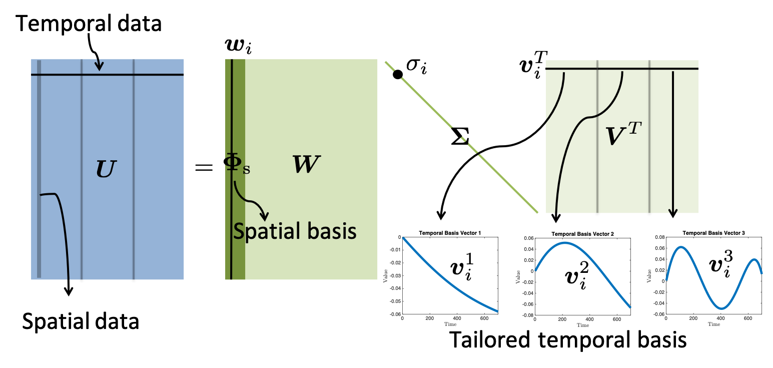
Figure 1: Illustration of spatial and temporal bases construction, using SVD with $n_{\mu}=3$. The right singular vector, $\boldsymbol{v}_{i}$, describes three different temporal behaviors of a left singular basis vector $\boldsymbol{w}_{i}$, i.e., three different temporal behaviors of a spatial mode. Each temporal behavior is denoted as $\boldsymbol{v}_{i}^{1}$, $\boldsymbol{v}_{i}^{2}$, and $\boldsymbol{v}_{i}^{3}$.

We follow the method of snapshots first introduced by Sirovich [35]. Let ${\mathcal{P}}=\{\boldsymbol{\mu}_{1},\ldots,\boldsymbol{\mu}_{n_{\mu}}\}$ be a set of parameter samples where we run full order model simulations. Let $\boldsymbol{U}_{p}\equiv\begin{bmatrix}\boldsymbol{u}^{(1)}(\boldsymbol{\mu}_{p})&\cdots&\boldsymbol{u}^{(N_{t})}(\boldsymbol{\mu}_{p})\end{bmatrix}\in\mathbb{R}^{N_{s}\times N_{t}}$, $p\in\mathbb{N}(n_{\mu})$, be a full order model state solution matrix for a sample parameter value, $\boldsymbol{\mu}_{p}\in\Omega_{\mu}$. Then a snapshot matrix, $\boldsymbol{U}\in\mathbb{R}^{N_{s}\times n_{\mu}N_{t}}$, is defined by concatenating all the state solution matrices, i.e.,

$$\boldsymbol{U}\equiv\begin{bmatrix}\boldsymbol{U}_{1}&\cdots&\boldsymbol{U}_{n_{\mu}}\end{bmatrix}.$$ (17)

The spatial basis from POD is an optimally compressed representation of $\text{range}(\boldsymbol{U})$ in a sense that it minimizes the difference between the original snapshot matrix and the projected one onto the subspace spanned by the basis, $\boldsymbol{\Phi}_{\text{s}}$:

$$\underset{\boldsymbol{\Phi}_{\text{s}}\in\mathbb{R}^{N_{s}\times n_{s}},\boldsymbol{\Phi}_{\text{s}}^{T}\boldsymbol{\Phi}_{\text{s}}=\boldsymbol{I}_{n_{s}}}{\text{minimize}} \left\|\boldsymbol{U}-\boldsymbol{\Phi}_{\text{s}}\boldsymbol{\Phi}_{\text{s}}^{T}{\boldsymbol{U}}\right\|_{F}^{2},$$ (18)

where $\|\cdot\|_{F}$ denotes the Frobenius norm. The solution of POD can be obtained by setting $\boldsymbol{\Phi}_{\text{s}}=\boldsymbol{W}(:,1:n_{s})$, $n_{s}<n_{\mu}N_{t}$, in MATLAB notation, where $\boldsymbol{W}$ is the left singular matrix of the following thin Singular Value Decomposition (SVD) with $\ell\equiv\min(N_{s},n_{\mu}N_{t})$:

$$\boldsymbol{U} =\boldsymbol{W}\boldsymbol{\Sigma}\boldsymbol{V}^{T}$$ (19)

$$=\sum_{i=1}^{\ell}\sigma_{i}\boldsymbol{w}_{i}\boldsymbol{v}_{i}^{T}$$ (20)

where $\boldsymbol{W}\in\mathbb{R}^{N_{s}\times\ell}$ and $\boldsymbol{V}\in\mathbb{R}^{n_{\mu}N_{t}\times\ell}$ are orthogonal matrices and $\boldsymbol{\Sigma}\in\mathbb{R}^{\ell\times\ell}$ is a diagonal matrix with singular values on its diagonal. The equivalent summation form is written in (20), where $\sigma_{i}\in\mathbb{R}$ is $i$th singular value, $\boldsymbol{w}_{i}$ and $\boldsymbol{v}_{i}$ are $i$th left and right singular vectors, respectively. Note that $\boldsymbol{v}_{i}$ describes $n_{\mu}$ different temporal behavior of $\boldsymbol{w}_{i}$. For example, Figure 1 illustrates the case of $n_{\mu}=3$, where $\boldsymbol{v}_{i}^{1}$, $\boldsymbol{v}_{i}^{2}$, and $\boldsymbol{v}_{i}^{3}$ describe three different temporal behavior of a specific spatial basis vector, i.e., $\boldsymbol{w}_{i}$. For general $n_{\mu}$, we note that $\boldsymbol{v}_{i}$ describes $n_{\mu}$ different temporal behavior of $i$th spatial basis vector, i.e., $\boldsymbol{\phi}^{\text{s}}_{i}=\boldsymbol{w}_{i}$. We set $\boldsymbol{\Upsilon}_{i}=\begin{bmatrix}\boldsymbol{v}_{i}^{1}&\cdots&\boldsymbol{v}_{i}^{n_{\mu}}\end{bmatrix}$ to be $i$th temporal snapshot matrix, where $\boldsymbol{v}_{i}^{k}\equiv\boldsymbol{v}_{i}(1+(k-1)N_{t}:kN_{t})$ for $k\in\mathbb{N}(n_{\mu})$. We apply SVD on $\boldsymbol{\Upsilon}_{i}$:

$$\boldsymbol{\Upsilon}_{i}=\boldsymbol{\Lambda}_{i}\boldsymbol{\Sigma}_{i}\boldsymbol{\Psi}_{i}^{T}.$$ (21)

Then, the temporal basis for $i$th spatial basis vector can be set $\boldsymbol{\Phi}_{\text{t}}^{i}=\boldsymbol{\Lambda}_{i}(:,1:n_{t})$ in MATLAB notation. Finally, a space–time basis vector, $\boldsymbol{\phi}^{\text{st}}_{i+n_{s}(j-1)}\in\mathbb{R}^{N_{s}N_{t}}$, in (14) can be constructed as

$$\boldsymbol{\phi}^{\text{st}}_{i+n_{s}(j-1)}=\boldsymbol{\phi}^{\text{t}}_{ij}\otimes\boldsymbol{\phi}^{\text{s}}_{i},$$ (22)

where $\boldsymbol{\phi}^{\text{s}}_{i}\equiv\boldsymbol{\Phi}_{\text{s}}(:,i)\in\mathbb{R}^{N_{s}}$ denotes $i$th spatial basis vector and $\boldsymbol{\phi}^{\text{t}}_{ij}\equiv\boldsymbol{\Phi}_{\text{t}}^{i}(:,j)\in\mathbb{R}^{N_{t}}$ denotes $j$th temporal basis vector that describes a temporal behavior of $\boldsymbol{\phi}^{\text{s}}_{i}$. The computational cost of SVD for the snapshot matrix, $\boldsymbol{U}\in\mathbb{R}^{N_{s}\times n_{\mu}N_{t}}$, assuming $N_{s}\gg n_{\mu}N_{t}$, is $O(N_{s}^{2}n_{\mu}N_{t})$ and the computational cost of SVD for $n_{s}$ temporal snapshot matrices, $\boldsymbol{\Upsilon}_{i}\in\mathbb{R}^{N_{t}\times n_{\mu}}$, $i\in\mathbb{N}(n_{s})$, $N_{t}\gg n_{\mu}$ is $O(N_{t}^{2}n_{s}n_{\mu})$. For a large-scale problem, this may be a formidable task. Thus, we use an incremental SVD where a rank one update of existing SVD is achieved with much more memory-efficient way than the thin SVD in Eq. (19). The incremental SVD procedure is explained in Section 4.2.

POD is related to the principal component analysis in statistics [22] and Karhunen–Loève expansion [26] in stochastic analysis. Since the objective function in (18) does not change even though $\boldsymbol{\Phi}_{\text{s}}$ is post-multiplied by an arbitrary $n_{s}\times n_{s}$ orthogonal matrix, the POD procedure seeks the optimal $n_{s}$-dimensional subspace that captures the snapshots in the least-squares sense. For more details on POD, we refer to [6, 21, 23].

4.2 Incremental space–time reduced basis

An incremental SVD is an efficient way of updating the existing singular value decomposition when a new snapshot vector, i.e., a column vector, is added. For a time dependent problem, we start with a first time step solution with a first parameter vector, i.e., $\boldsymbol{u}^{(1)}(\boldsymbol{\mu}_{1})$. If its norm is big enough (i.e., $\|\boldsymbol{u}^{(1)}(\boldsymbol{\mu}_{1})\|>\epsilon_{\text{SVD}}$), then we set the first singular value $\sigma_{1}=\|\boldsymbol{u}^{(1)}(\boldsymbol{\mu}_{1})\|$, the first left singular vector be the normalized first snapshot vector, i.e., $\boldsymbol{w}_{1}=\boldsymbol{u}^{(1)}(\boldsymbol{\mu}_{1})/\sigma_{1}$, and the right singular vector be $\boldsymbol{v}_{1}=1$. Otherwise, we set them empty, i.e., $\sigma_{1}=[]$, $\boldsymbol{w}_{1}=[]$, and $\boldsymbol{v}_{1}=[]$. This initializing process is described in Algorithm 1. We pass $k$ to initializingIncrementalSVD function as an input argument to indicate $k$th snapshot vector is being handled. Also, the rank of $\boldsymbol{W}_{k}$ is denoted as $r_{k}$. In general, $r_{k}\neq k$ because a snapshot vector will not be included if it is too small (i.e., Line 1 in Algorithm 1) or it is linearly dependent on the existing basis (i.e., Line 9 and 13 in Algorithm 2) or it generates a small eigenvalue (i.e., Line 18 in Algorithm 2).

Let’s assume that we have $(k-1)$th SVD from previous $k-1$ snapshot vectors, i.e., $\boldsymbol{W}_{k-1}\boldsymbol{\Sigma}_{k-1}\boldsymbol{V}_{k-1}^{T}$, whose rank is $r_{k-1}$. If a new snapshot vector, $\boldsymbol{u}$ (e.g., $k$th time step solution with the first sample parameter value, $\boldsymbol{u}^{(k)}(\boldsymbol{\mu}_{1})$) needs to be added to the existing SVD, the following factorization can be used [9]:

$$\begin{bmatrix}\boldsymbol{W}_{k-1}\boldsymbol{\Sigma}_{k-1}\boldsymbol{V}_{k-1}^{T}&\boldsymbol{u}\end{bmatrix} =\begin{bmatrix}\boldsymbol{W}_{k-1}&\left(\boldsymbol{I}-\boldsymbol{W}_{k-1}\boldsymbol{W}_{k-1}^{T}\right)\boldsymbol{u}/p\end{bmatrix}\begin{bmatrix}\boldsymbol{\Sigma}_{k-1}&\boldsymbol{W}_{k-1}^{T}\boldsymbol{u}\\ \boldsymbol{0}&p\end{bmatrix}\begin{bmatrix}\boldsymbol{V}_{k-1}&\boldsymbol{0}\\ \boldsymbol{0}&1\end{bmatrix}^{T}$$ (23)

$$=\begin{bmatrix}\boldsymbol{W}_{k-1}&\boldsymbol{j}\end{bmatrix}\begin{bmatrix}\boldsymbol{\Sigma}_{k-1}&\boldsymbol{\ell}\\ \boldsymbol{0}&p\end{bmatrix}\begin{bmatrix}\boldsymbol{V}_{k-1}&\boldsymbol{0}\\ \boldsymbol{0}&1\end{bmatrix}^{T},$$ (24)

where $\boldsymbol{\ell}=\boldsymbol{W}_{k-1}^{T}\boldsymbol{u}\in\mathbb{R}^{r_{k-1}}$ denotes a reduced coordinate of $\boldsymbol{u}$ that is projected onto the subspace spanned by $\boldsymbol{W}_{k-1}$, $p=\|\boldsymbol{u}-\boldsymbol{W}_{k-1}\boldsymbol{\ell}\|$ denotes the norm of the difference between $\boldsymbol{u}$ and the projected one, and $\boldsymbol{j}=\left(\boldsymbol{u}-\boldsymbol{W}_{k-1}\boldsymbol{\ell}\right)/p\in\mathbb{R}^{N_{s}}$ denotes a new orthogonal vector due to the incoming vector, $\boldsymbol{u}$. Note that the left and right matrices of the factorization, i.e., $\begin{bmatrix}\boldsymbol{W}_{k-1}&\boldsymbol{j}\end{bmatrix}\in\mathbb{R}^{N_{s}\times(r_{k-1}+1)}$ and $\begin{bmatrix}\boldsymbol{V}_{k-1}&\boldsymbol{0}\\ \boldsymbol{0}&1\end{bmatrix}\in\mathbb{R}^{k\times(r_{k-1}+1)}$ are orthogonal matrices. Let $\boldsymbol{Q}\in{\mathbb{R}^{(r_{k-1}+1)\times(r_{k-1}+1)}}$ denote the middle matrix of the factorization, i.e.,

$$\boldsymbol{Q}=\begin{bmatrix}\boldsymbol{\Sigma}_{k-1}&\boldsymbol{\ell}\\ \boldsymbol{0}&p\end{bmatrix}.$$ (25)

The matrix, $\boldsymbol{Q}$, is almost diagonal except for $\boldsymbol{\ell}$ in the upper right block, i.e., one column bordered diagonal. Its size is not in $O(N_{s})$. Thus, the SVD of $\boldsymbol{Q}$ is computationally cheap, i.e., $O((r_{k-1}+1)^{3})$. Let the SVD of $\boldsymbol{Q}$ be

$$\boldsymbol{Q}=\mkern 1.5mu\overline{\mkern-1.5mu\boldsymbol{W}\mkern-1.5mu}\mkern 1.5mu\mkern 1.5mu\overline{\mkern-1.5mu\boldsymbol{\Sigma}\mkern-1.5mu}\mkern 1.5mu\mkern 1.5mu\overline{\mkern-1.5mu\boldsymbol{V}\mkern-1.5mu}\mkern 1.5mu,$$ (26)

where $\mkern 1.5mu\overline{\mkern-1.5mu\boldsymbol{W}\mkern-1.5mu}\mkern 1.5mu\in\mathbb{R}^{(r_{k-1}+1)\times(r_{k-1}+1)}$ denotes the left singular matrix, $\mkern 1.5mu\overline{\mkern-1.5mu\boldsymbol{\Sigma}\mkern-1.5mu}\mkern 1.5mu\in\mathbb{R}^{(r_{k-1}+1)\times(r_{k-1}+1)}$ denotes the singular value matrix, and $\mkern 1.5mu\overline{\mkern-1.5mu\boldsymbol{V}\mkern-1.5mu}\mkern 1.5mu\in\mathbb{R}^{(r_{k-1}+1)\times(r_{k-1}+1)}$ denotes the right singular matrix of $\boldsymbol{Q}$. Replacing $\boldsymbol{Q}$ in Eq. (24) with (26) gives

$$\begin{bmatrix}\boldsymbol{W}_{k-1}\boldsymbol{\Sigma}_{k-1}\boldsymbol{V}_{k-1}^{T}&\boldsymbol{u}\end{bmatrix} =\begin{bmatrix}\boldsymbol{W}_{k-1}&\boldsymbol{j}\end{bmatrix}\mkern 1.5mu\overline{\mkern-1.5mu\boldsymbol{W}\mkern-1.5mu}\mkern 1.5mu\mkern 1.5mu\overline{\mkern-1.5mu\boldsymbol{\Sigma}\mkern-1.5mu}\mkern 1.5mu\mkern 1.5mu\overline{\mkern-1.5mu\boldsymbol{V}\mkern-1.5mu}\mkern 1.5mu\begin{bmatrix}\boldsymbol{V}_{k-1}&\boldsymbol{0}\\ \boldsymbol{0}&1\end{bmatrix}^{T}$$ (27)

$$=\boldsymbol{W}_{k}\boldsymbol{\Sigma}_{k}\boldsymbol{V}_{k}^{T},$$ (28)

where $\boldsymbol{W}_{k}=\begin{bmatrix}\boldsymbol{W}_{k-1}&\boldsymbol{j}\end{bmatrix}\mkern 1.5mu\overline{\mkern-1.5mu\boldsymbol{W}\mkern-1.5mu}\mkern 1.5mu\in\mathbb{R}^{N_{s}\times(r_{k-1}+1)}$ denotes the updated left singular matrix, $\boldsymbol{\Sigma}_{k}=\mkern 1.5mu\overline{\mkern-1.5mu\boldsymbol{\Sigma}\mkern-1.5mu}\mkern 1.5mu\in\mathbb{R}^{(r_{k-1}+1)\times(r_{k-1}+1)}$ denotes the updated singular value matrix, and $\boldsymbol{V}_{k}=\begin{bmatrix}\boldsymbol{V}_{k-1}&\boldsymbol{0}\\ \boldsymbol{0}&1\end{bmatrix}\mkern 1.5mu\overline{\mkern-1.5mu\boldsymbol{V}\mkern-1.5mu}\mkern 1.5mu\in\mathbb{R}^{k\times(r_{k-1}+1)}$ denotes the updated right singular matrix. This updating algorithm is described in Algorithm 2.

Algorithm 2 also checks if $\boldsymbol{u}$ is linearly dependent on the current left singular vectors numerically. If $p<\epsilon_{\text{SVD}}$, then we consider that it is linearly dependent. Thus, we set $p=0$ in $\boldsymbol{Q}$, i.e., Line 10 of Algorithm 2. Then we only update the first $r_{k-1}$ components of the singular matrices in Line 14 of Algorithm 2. Otherwise, we follow the update form in Eq. (28) as in Line 16 in Algorithm 2.

Line 18-20 in Algorithm 2 checks if the updated singular value has a small value. If it does, we neglect that particular singular value and corresponding component in left and right singular matrices. It is because a small singular value causes a large error in left and right singular matrices [18].

Although the orthogonality of the updated left singular matrix, $\boldsymbol{W}_{k}$, must be guaranteed in infinite precision by the product of two orthogonal matrices in Line 14 or 16 of Algorithm 2, it is not guaranteed in finite precision. Thus, we heuristically check the orthogonality in Lines 21-24 of Algorithm 2 by checking the inner product of the first and last columns of $\boldsymbol{\Phi}_{k}$. If the orthogonality is not shown, then we orthogonalize them by the QR factorization. Here $\epsilon$ denotes unit roundoff (e.g., eps in MATLAB).

The spatial basis can be set after $n_{\mu}N_{t}$ incremental steps:

$$\boldsymbol{\Phi}_{\text{s}}=\boldsymbol{W}_{n_{\mu}N_{t}}(:,1:n_{s}).$$ (29)

If all the time step solutions are taken incrementally and sequentially from $n_{\mu}$ different high-fidelity time dependent simulations, then the right singular matrix, $\boldsymbol{V}_{N_{t}n_{\mu}}\in\mathbb{R}^{N_{t}n_{\mu}\times r_{N_{t}n_{\mu}}}$, holds $n_{\mu}$ different temporal behavior for each spatial basis vector. For example, $\boldsymbol{v}_{i}$ describes $n_{\mu}$ different temporal behavior of $\boldsymbol{w}_{i}$. As in Section 4.1, $i$th temporal snapshot matrix $\boldsymbol{\Upsilon}_{i}\in\mathbb{R}^{N_{t}\times n_{\mu}}$ can be defined as

$$\boldsymbol{\Upsilon}_{i}\equiv\begin{bmatrix}\boldsymbol{v}_{i}^{1}&\cdots&\boldsymbol{v}_{i}^{n_{\mu}}\end{bmatrix},$$ (30)

where $\boldsymbol{v}_{i}^{k}\equiv\boldsymbol{V}_{N_{t}n_{\mu}}(1+(k-1)N_{t}:kN_{t},i)$ for $k\in\mathbb{N}(n_{\mu})$. If we take the SVD of $\boldsymbol{\Upsilon}_{i}=\boldsymbol{\Lambda}_{i}\boldsymbol{\Sigma}_{i}\boldsymbol{\Psi}_{i}^{T}$, then the temporal basis for $i$th spatial basis vector can be set

$$\boldsymbol{\Phi}_{\text{t}}^{i}=\boldsymbol{\Lambda}_{i}(:,1:n_{t}).$$ (31)

Algorithm 1 Initializing incremental SVD

[$\boldsymbol{W}_{k}$, $\boldsymbol{\sigma}_{k}$, $\boldsymbol{V}_{k}$] = initializingIncrementalSVD($\boldsymbol{u}$, $\epsilon_{\text{SVD}}$, $k$)
Input: $\boldsymbol{u}$, $\epsilon_{\text{SVD}}$, $k$
Output: $\boldsymbol{W}_{k}$, $\boldsymbol{\sigma}_{k}$, $\boldsymbol{V}_{k}$

1:  if $\|\boldsymbol{u}\|>\epsilon_{\text{SVD}}$ then

2:     $\boldsymbol{\sigma}_{k}\leftarrow\begin{bmatrix}\|\boldsymbol{u}\|\end{bmatrix}$, $\boldsymbol{W}_{k}\leftarrow\boldsymbol{u}/\sigma_{1}$, and $\boldsymbol{V}_{k}\leftarrow\begin{bmatrix}1\end{bmatrix}$

3:  else

4:     $\boldsymbol{\sigma}_{k}\leftarrow[]$, $\boldsymbol{W}_{k}\leftarrow[]$, and $\boldsymbol{V}_{k}\leftarrow[]$

5:  end if

Algorithm 2 Incremental SVD, $\boldsymbol{W}_{-1}=[]$

[$\boldsymbol{W}_{k}$, $\boldsymbol{\sigma}_{k}$, $\boldsymbol{V}_{k}$] = incrementalSVD($\boldsymbol{u}$, $\epsilon_{\text{SVD}}$, $\epsilon_{\text{SV}}$, $\boldsymbol{W}_{k-1}$, $\boldsymbol{\sigma}_{k}$, $\boldsymbol{V}_{k-1}$, $k$)
Input: $\boldsymbol{u}$, $\epsilon_{\text{SVD}}$, $\epsilon_{\text{SV}}$, $\boldsymbol{W}_{k-1}$, $\boldsymbol{\sigma}_{k-1}$, $\boldsymbol{V}_{k-1}$, $k$
Output: $\boldsymbol{W}_{k}$, $\boldsymbol{\sigma}_{k}$, $\boldsymbol{V}_{k}$

1:  if $r_{k-1}=0$ or $r_{k-1}=r_{\text{max}}$ then

2:     [$\boldsymbol{W}_{k}$, $\boldsymbol{\sigma}_{k}$, $\boldsymbol{V}_{k}$] = initializingIncrementalSVD($\boldsymbol{u}$, $\epsilon_{\text{SVD}}$, $k$), i.e., apply Algorithm 1

3:     return  

4:  end if

5:  $\boldsymbol{\boldsymbol{\ell}}\leftarrow\boldsymbol{W}_{k-1}^{T}\boldsymbol{u}$

6:  $p\leftarrow\sqrt{\boldsymbol{u}^{T}\boldsymbol{u}-\boldsymbol{\ell}^{T}\boldsymbol{\ell}}$

7:  $\boldsymbol{j}\leftarrow(\boldsymbol{u}-\boldsymbol{W}_{k-1}\boldsymbol{\ell})/p$

8:  $\boldsymbol{Q}\leftarrow\begin{bmatrix}\text{diag}(s)&\boldsymbol{\ell}\\ \boldsymbol{0}&p\end{bmatrix}$

9:  if $p<\epsilon_{\text{SVD}}$ then

10:     $\boldsymbol{Q}_{\text{end},\text{end}}\leftarrow 0$

11:  end if

12:  $[\mkern 1.5mu\overline{\mkern-1.5mu\boldsymbol{W}\mkern-1.5mu}\mkern 1.5mu,\mkern 1.5mu\overline{\mkern-1.5mu\boldsymbol{\Sigma}\mkern-1.5mu}\mkern 1.5mu,\mkern 1.5mu\overline{\mkern-1.5mu\boldsymbol{V}\mkern-1.5mu}\mkern 1.5mu]\leftarrow\text{SVD}(\boldsymbol{Q})$ $\#$ SVD update

13:  if $p<\epsilon_{\text{SVD}}$ then

14:     $\boldsymbol{W}_{k}\leftarrow\boldsymbol{W}_{k-1}{\mkern 1.5mu\overline{\mkern-1.5mu\boldsymbol{W}\mkern-1.5mu}\mkern 1.5mu}_{(1:r_{k-1},1:r_{k-1})}$,  $\boldsymbol{\sigma}_{k}\leftarrow\text{diag}(\mkern 1.5mu\overline{\mkern-1.5mu\boldsymbol{\Sigma}\mkern-1.5mu}\mkern 1.5mu_{(1:r_{k-1},1:r_{k-1})})$, and $\boldsymbol{V}_{k}\leftarrow\begin{bmatrix}\boldsymbol{V}_{k}&\boldsymbol{0}\\ \boldsymbol{0}&1\end{bmatrix}{\mkern 1.5mu\overline{\mkern-1.5mu\boldsymbol{V}\mkern-1.5mu}\mkern 1.5mu}_{(:,1:r_{k-1})}$

15:  else

16:     $\boldsymbol{W}_{k}\leftarrow\begin{bmatrix}\boldsymbol{W}_{k-1}&\boldsymbol{j}\end{bmatrix}\mkern 1.5mu\overline{\mkern-1.5mu\boldsymbol{W}\mkern-1.5mu}\mkern 1.5mu$,  $\boldsymbol{\sigma}_{k}\leftarrow\text{diag}(\mkern 1.5mu\overline{\mkern-1.5mu\boldsymbol{\Sigma}\mkern-1.5mu}\mkern 1.5mu)$,  and $\boldsymbol{V}_{k}\leftarrow\begin{bmatrix}\boldsymbol{V}_{k}&\boldsymbol{0}\\ \boldsymbol{0}&1\end{bmatrix}\mkern 1.5mu\overline{\mkern-1.5mu\boldsymbol{V}\mkern-1.5mu}\mkern 1.5mu$

17:  end if$\#$ Neglect small singular values: truncation

18:  if ${\boldsymbol{\sigma}_{k}}_{(r_{k})}<\epsilon_{\text{SV}}$ then

19:     $\boldsymbol{\sigma}_{k}\leftarrow{\boldsymbol{\sigma}_{k}}_{(1:r_{k}-1)}$,  $\boldsymbol{W}_{k}\leftarrow{\boldsymbol{W}_{k}}_{(:,1:r_{k}-1)}$,  $\boldsymbol{V}_{k}\leftarrow{\boldsymbol{V}_{k}}_{(:,1:r_{k}-1)}$

20:  end if$\#$ Orthogonalize if necessary

21:  if ${\boldsymbol{W}_{k}}^{T}_{(:,1)}{\boldsymbol{W}_{k}}_{(:,\text{end})}>\min\{\epsilon_{\text{SVD}},\epsilon\cdot N_{s}\}$ then

22:     $[\mkern 1.5mu\overline{\mkern-1.5mu\boldsymbol{Q}\mkern-1.5mu}\mkern 1.5mu,\boldsymbol{R}]\leftarrow QR\{\boldsymbol{W}_{k}\}$

23:     $\boldsymbol{W}_{k}\leftarrow\mkern 1.5mu\overline{\mkern-1.5mu\boldsymbol{Q}\mkern-1.5mu}\mkern 1.5mu$

24:  end if

4.3 Space–time reduced basis in block structure

Forming the space–time basis in Eq. (14) through the the Kronecker product in Eq. (22) requires $N_{s}N_{t}n_{s}n_{t}$ multiplications. This is troublesome, not only because it is computationally costly, but also it requires too much memory. Fortunately, a block structure of the space–time basis in (14) is available:

$$\boldsymbol{\Phi}_{st}=\begin{bmatrix}\boldsymbol{\Phi}_{\text{s}}\boldsymbol{D}_{1}^{1}&\cdots&\cdots&\cdots&\boldsymbol{\Phi}_{\text{s}}\boldsymbol{D}_{1}^{n_{t}}\\ \vdots&\ddots&\vdots&\cdot^{\cdot^{\cdot}}&\vdots\\ \vdots&\ldots&\boldsymbol{\Phi}_{\text{s}}\boldsymbol{D}_{k}^{j}&\ldots&\vdots\\ \vdots&\cdot^{\cdot^{\cdot}}&\vdots&\ddots&\vdots\\ \boldsymbol{\Phi}_{\text{s}}\boldsymbol{D}_{N_{t}}^{1}&\cdots&\cdots&\cdots&\boldsymbol{\Phi}_{\text{s}}\boldsymbol{D}_{N_{t}}^{n_{t}}\\ \end{bmatrix}\in\mathbb{R}^{N_{s}N_{t}\times n_{s}n_{t}},$$ (32)

where $k$th time step temporal basis matrix, $\boldsymbol{D}_{k}^{j}\in\mathbb{R}^{n_{s}\times n_{s}}$, is defined as

$$\boldsymbol{D}_{k}^{j}\equiv\text{diag}\left(\begin{bmatrix}\phi^{\text{t}}_{1j,k}&\cdots&\phi^{\text{t}}_{n_{s}j,k}\end{bmatrix}\right),$$ (33)

where $\phi^{\text{t}}_{ij,k}\in\mathbb{R}$ denotes a $k$th element of $\boldsymbol{\phi}^{\text{t}}_{ij}$. Thanks to this block structure, the space–time reduced order operators, such as $\hat{\boldsymbol{A}}^{\text{st}}$, $\hat{\boldsymbol{f}}^{\text{st}}$, and $\hat{\boldsymbol{u}}_{0}^{\text{st}}$ can be formed without explicitly forming $\boldsymbol{\Phi}_{\text{st}}$. For example, the reduced space–time system matrix, $\hat{\boldsymbol{A}}^{\text{st}}$ can be computed, using the block structures, as

$$\hat{\boldsymbol{A}}^{\text{st}}(\boldsymbol{\mu})=\boldsymbol{\Phi}_{\text{st}}^{T}\boldsymbol{A}^{\text{st}}(\boldsymbol{\mu})\boldsymbol{\Phi}_{\text{st}}=\begin{bmatrix}\hat{\boldsymbol{A}}^{\text{st}}_{(1,1)}(\boldsymbol{\mu})&\cdots&\cdots&\cdots&\hat{\boldsymbol{A}}^{\text{st}}_{(1,n_{t})}(\boldsymbol{\mu})\\ \vdots&\ddots&\vdots&\cdot^{\cdot^{\cdot}}&\vdots\\ \vdots&\cdots&\hat{\boldsymbol{A}}^{\text{st}}_{(j^{\prime},j)}(\boldsymbol{\mu})&\cdots&\vdots\\ \vdots&\cdot^{\cdot^{\cdot}}&\vdots&\ddots&\vdots\\ \hat{\boldsymbol{A}}^{\text{st}}_{(n_{t},1)}(\boldsymbol{\mu})&\cdots&\cdots&\cdots&\hat{\boldsymbol{A}}^{\text{st}}_{(n_{t},n_{t})}(\boldsymbol{\mu})\end{bmatrix},$$ (34)

where ($j^{\prime}$,$j$)th block matrix, $\hat{\boldsymbol{A}}^{\text{st}}_{(j^{\prime},j)}(\boldsymbol{\mu})\in\mathbb{R}^{n_{s}\times n_{s}}$, $j^{\prime}$, $j\in\mathbb{N}(n_{t})$ is defined as

$$\hat{\boldsymbol{A}}^{\text{st}}_{(j^{\prime},j)}(\boldsymbol{\mu})=\sum_{k=1}^{N_{t}}\left(\boldsymbol{D}_{k}^{j^{\prime}}\boldsymbol{D}_{k}^{j}-\Delta t^{(k)}\boldsymbol{D}_{k}^{j^{\prime}}\hat{\boldsymbol{A}}(\boldsymbol{\mu})\boldsymbol{D}_{k}^{j}\right)-\sum_{k=1}^{N_{t}-1}\boldsymbol{D}_{k+1}^{j^{\prime}}\boldsymbol{D}_{k}^{j}.$$ (35)

Note that the computations of $\boldsymbol{D}_{k}^{j^{\prime}}\boldsymbol{D}_{k}^{j}$ and $\boldsymbol{D}_{k+1}^{j^{\prime}}\boldsymbol{D}_{k}^{j}$ are trivial because they are diagonal matrix-products whose individual product requires $n_{s}$ scalar products. Additionally, $\hat{\boldsymbol{A}}:\mathbb{R}^{n_{\mu}}\rightarrow\mathbb{R}^{n_{s}\times n_{s}}$, is a reduced order system operator that is used for the spatial ROMs, e.g., see Eq. (10). This can be pre-computed. It implies that the construction of $\hat{\boldsymbol{A}}^{\text{st}}(\boldsymbol{\mu})$ requires computational cost that is a bit larger than the one for the spatial ROM system matrix. The additional cost $O(n_{s}^{2}n_{t}^{2}N_{t})$ to the spatial ROM system matrix construction is required.

Similarly, the reduced space–time input vector, $\hat{\boldsymbol{f}}^{\text{st}}\in\mathbb{R}^{n_{s}n_{t}}$, can be computed as

$$\hat{\boldsymbol{f}}^{\text{st}}=\boldsymbol{\Phi}_{\text{st}}^{T}\boldsymbol{f}^{\text{st}}=\begin{bmatrix}\vdots\\ \hat{\boldsymbol{f}}^{\text{st}}_{(j)}\\ \vdots\end{bmatrix},$$ (36)

where the $j$th block vector, $\hat{\boldsymbol{f}}^{\text{st}}_{(j)}\in\mathbb{R}^{n_{s}}$, $j\in\mathbb{N}(n_{t})$, is given as

$$\hat{\boldsymbol{f}}^{\text{st}}_{(j)}(\boldsymbol{\mu})=\sum_{k=1}^{N_{t}}\Delta t^{(k)}\boldsymbol{D}_{k}^{j}\hat{\boldsymbol{B}}(\boldsymbol{\mu})\boldsymbol{f}^{(k)}.$$ (37)

Note that $\hat{\boldsymbol{B}}:\mathbb{R}^{n_{\mu}}\rightarrow\mathbb{R}^{n_{s}\times N_{i}}$ is used for the spatial ROMs, e.g., see Eq. (10). Also, $\hat{\boldsymbol{B}}(\boldsymbol{\mu})\boldsymbol{f}^{(k)}$ needs to be computed in the spatial ROMs. These can be pre-computed. Other operations are related to the row-wise scaling with diagonal term, $\boldsymbol{D}_{k}^{j}$, whose computational cost is $O(n_{s}n_{t}N_{t})$. If $\boldsymbol{f}^{(k)}$ is constant throughout the whole time steps, i.e., $\boldsymbol{f}^{(k)}=\boldsymbol{f}$, then Eq. (37) can be further reduced to

$$\hat{\boldsymbol{f}}^{\text{st}}_{(j)}(\boldsymbol{\mu})=\left(\sum_{k=1}^{N_{t}}\Delta t^{(k)}\boldsymbol{D}_{k}^{j}\right)\hat{\boldsymbol{B}}(\boldsymbol{\mu})\boldsymbol{f},$$ (38)

where you can compute the summation term first, then multiply the diagonal term with the precomputed term, $\hat{\boldsymbol{B}}\boldsymbol{f}$, which is not much more than the cost for constructing the reduced input vector for the spatial ROM.

Finally, the space–time initial vector, $\hat{\boldsymbol{u}}_{0}^{\text{st}}\in\mathbb{R}^{n_{s}n_{t}}$, can be computed as

$$\hat{\boldsymbol{u}}_{0}^{\text{st}}=\boldsymbol{\Phi}_{\text{st}}^{T}\boldsymbol{u}_{0}^{\text{st}}=\begin{bmatrix}\hat{\boldsymbol{u}}_{0,1}^{\text{st}}\\ \boldsymbol{0}\\ \vdots\\ \boldsymbol{0}\end{bmatrix},$$ (39)

where the first block vector, $\hat{\boldsymbol{u}}_{0,1}^{\text{st}}\in\mathbb{R}^{n_{s}}$, is given as

$$\hat{\boldsymbol{u}}_{0,1}^{\text{st}}=\left(\sum_{k=1}^{N_{t}}\boldsymbol{D}_{k}^{1}\right)\hat{\boldsymbol{u}}_{0}.$$ (40)

Note that $\hat{\boldsymbol{u}}_{0}\in\mathbb{R}^{n_{s}}$ is the reduced initial condition in the spatial ROM, e.g., see Eq. (10). The additional cost to construct the space–time reduced initial vector is $O(n_{s})$.

In summary, the block structure in Eq. (32) enables the block term expression of the space–time reduced operators, i.e., $\hat{\boldsymbol{A}}^{\text{st}}$, $\hat{\boldsymbol{f}}^{\text{st}}$, and $\hat{\boldsymbol{u}}_{0}^{\text{st}}$, which results in a comparable computational cost that is not much more expensive than the construction of the spatial reduced operators, i.e., $\hat{\boldsymbol{A}}$, $\hat{\boldsymbol{B}}$, and $\hat{\boldsymbol{u}}_{0}$. This fact attracts the desire to use the spatio-temporal ROM rather than spatial ROM because the spatio-temporal ROM solving time is much smaller than the corresponding spatial ROM.

5 Error analysis

The error analysis for spatial and spatio-temporal ROMs is presented in this section. Section 5.1 presents two error bounds for the spatial ROM, while Section 5.2 presents error bounds for the spatio-termporal ROM.

5.1 Error analysis for the spatial ROM

First, two error bounds will be derived for the spatial ROM presented in Section 3.1. We define residual function for $k$th time step FOM, $\boldsymbol{r}^{(k)}:\mathbb{R}^{N_{s}}\times\mathbb{R}^{N_{s}}\rightarrow\mathbb{R}^{N_{s}}$, as

$$\boldsymbol{r}^{(k)}\left(\boldsymbol{u}^{(k)},\boldsymbol{u}^{(k-1)}\right)\equiv\boldsymbol{u}^{(k)}-\boldsymbol{u}^{(k-1)}-\Delta t^{(k)}\boldsymbol{A}\boldsymbol{u}^{(k)}-\Delta t^{(k)}\boldsymbol{B}\boldsymbol{f}^{(k)},$$ (41)

which is zero if $\boldsymbol{u}^{(k)}$ and $\boldsymbol{u}^{(k-1)}$ are FOM solutions from Eq. (3). Here, we drop the parameter dependence for brevity. Let $\tilde{\boldsymbol{u}}^{(k)}\in\mathbb{R}^{N_{s}}$ be the solution approximation at $k$th time step due to the spatial ROM, i.e., $\tilde{\boldsymbol{u}}^{(k)}=\boldsymbol{u}_{\text{ref}}+\boldsymbol{\Phi}_{\text{s}}\hat{\boldsymbol{u}}^{(k)}$. Note that the approximate solutions make the following approximate residual function zero:

$$\boldsymbol{0}=\tilde{\boldsymbol{r}}^{(k)}\left(\tilde{\boldsymbol{u}}^{(k)},\tilde{\boldsymbol{u}}^{(k-1)}\right)\equiv\tilde{\boldsymbol{u}}^{(k)}-\tilde{\boldsymbol{u}}^{(k-1)}-\Delta t^{(k)}\boldsymbol{\Phi}_{\text{s}}\boldsymbol{\Phi}_{\text{s}}^{T}\boldsymbol{A}\tilde{\boldsymbol{u}}^{(k)}-\Delta t^{(k)}\boldsymbol{\Phi}_{\text{s}}\boldsymbol{\Phi}_{\text{s}}^{T}\boldsymbol{B}\boldsymbol{f}^{(k)}.$$ (42)

Throughout this section, we use the following notations: $\delta\boldsymbol{u}^{(k)}\equiv\boldsymbol{u}^{(k)}-\tilde{\boldsymbol{u}}^{(k)}$, $\boldsymbol{P}\equiv\boldsymbol{\Phi}_{\text{s}}\boldsymbol{\Phi}_{\text{s}}^{T}$, and $\boldsymbol{T}_{k}\equiv\boldsymbol{I}_{N_{s}}-\Delta t^{(k)}\boldsymbol{A}$.

Theorem 1

(a residual-based a posteriori error bound with the backward Euler time integrator) Let $\alpha_{k}\in\mathbb{R}$ be a matrix norm of the inverse of the backward Euler time integrator operator, i.e., $\alpha_{k}\equiv\left\|\boldsymbol{T}_{k}^{-1}\right\|_{2}$. Then, a residual-based a posteriori error bound at $k$th time step is given as

$${\displaystyle\left\|\delta\boldsymbol{u}^{(k)}\right\|_{2}\leq\sum_{i=1}^{k}L_{i}\left\|\boldsymbol{r}^{(i)}\left(\tilde{\boldsymbol{u}}^{(i)},\tilde{\boldsymbol{u}}^{(i-1)}\right)\right\|_{2}},$$ (43)

where the stability constants, $L_{i}\in\mathbb{R}$, are defined as $L_{i}\equiv\prod_{j=i}^{k}\alpha_{j}$.

Proof. Approximate solutions, $\tilde{\boldsymbol{u}}^{(k)}$ and $\tilde{\boldsymbol{u}}^{(k-1)}$, make the residual nonzero and it can be expanded as

$$-\boldsymbol{r}^{(k)}\left(\tilde{\boldsymbol{u}}^{(k)},\tilde{\boldsymbol{u}}^{(k-1)}\right) =\boldsymbol{r}^{(k)}\left(\boldsymbol{u}^{(k)},\boldsymbol{u}^{(k-1)}\right)-\boldsymbol{r}^{(k)}\left(\tilde{\boldsymbol{u}}^{(k)},\tilde{\boldsymbol{u}}^{(k-1)}\right)$$ (44)

$$=\delta\boldsymbol{u}^{(k)}-\delta\boldsymbol{u}^{(k-1)}-\Delta t^{(k)}\boldsymbol{A}\delta\boldsymbol{u}^{(k)},$$ (45)

where we have used the fact that $\boldsymbol{r}^{(k)}\left(\boldsymbol{u}^{(k)},\boldsymbol{u}^{(k-1)}\right)=\boldsymbol{0}$. Rearranging terms and inverting the time integrator operator gives

$$\delta\boldsymbol{u}^{(k)}=\boldsymbol{T}_{k}^{-1}\left[\delta\boldsymbol{u}^{(k-1)}-\boldsymbol{r}^{(k)}\left(\tilde{\boldsymbol{u}}^{(k)},\tilde{\boldsymbol{u}}^{(k-1)}\right)\right].$$ (46)

Taking a norm each side, applying triangle inequality and Hölder’s inequality, we obtain the following one-time step bound:

$$\left\|\delta\boldsymbol{u}^{(k)}\right\|_{2}\leq\alpha_{k}\left(\left\|\delta\boldsymbol{u}^{(k-1)}\right\|_{2}+\left\|\boldsymbol{r}^{(k)}\left(\tilde{\boldsymbol{u}}^{(k)},\tilde{\boldsymbol{u}}^{(k-1)}\right)\right\|_{2}\right)$$ (47)

Assuming $\tilde{\boldsymbol{u}}^{(0)}=\boldsymbol{u}^{(0)}$, which can be achieved by setting $\boldsymbol{u}_{\text{ref}}=\boldsymbol{u}^{(0)}$, and applying (47) recursively, we get the claimed bound, i.e., (43).          

It is easy to see that the error bound in (43) is exponentially increasing with respect to time because of the summation and product appeared in the definition of stability constants, i.e., $L_{i}$. For $\ell_{2}$ induced matrix norm, $\alpha_{k}$ is the reciprocal of the smallest singular value of $\boldsymbol{T}_{k}$. Also, the error bound in (43) allows any approximate solution, that is, $\tilde{\boldsymbol{u}}^{(k)}$ does not need to come from the spatial ROM solution. The next theorem, however, shows an error bound for a specific case, i.e., the error bound for the spatial ROM solutions.

Theorem 2

(a spatial ROM-specific a posteriori error bound with the backward Euler time integrator) Let $\beta_{k}\in\mathbb{R}$ be defined as $\beta_{k}\equiv 1/\left(1-\Delta t^{(k)}\|\boldsymbol{A}\|_{2}\right)$. Also, assume that the timestep, $\Delta t^{(k)}$, is sufficiently small, i.e., $\Delta t^{(k)}<1/\|\boldsymbol{A}\|_{2}$. Then, a spatial ROM-specific a posteriori error bound at $k$th time step is given as

$${\displaystyle\left\|\delta\boldsymbol{u}^{(k)}\right\|_{2}\leq\sum_{i=1}^{k}M_{i}\left\|\boldsymbol{q}_{i}\right\|_{2}},$$ (48)

where the stability constants, $M_{i}\in\mathbb{R}$, are defined as $M_{i}\equiv\prod_{j=i}^{k}\beta_{j}$, and $\boldsymbol{q}_{k}\in\mathbb{R}^{N_{s}}$ be defined as $\boldsymbol{q}_{i}\equiv\Delta t^{(i)}\left(\boldsymbol{A}\tilde{\boldsymbol{u}}^{(i)}+\boldsymbol{B}\boldsymbol{f}^{(i)}\right)$.

Proof. Substracting Eq. (41) by Eq. (42) gives

$$\boldsymbol{0} =\boldsymbol{r}^{(k)}\left(\boldsymbol{u}^{(k)},\boldsymbol{u}^{(k-1)}\right)-\tilde{\boldsymbol{r}}^{(k)}\left(\tilde{\boldsymbol{u}}^{(k)},\tilde{\boldsymbol{u}}^{(k-1)}\right)$$ (49)

$$=\delta\boldsymbol{u}^{(k)}-\delta\boldsymbol{u}^{(k-1)}-\Delta t^{(k)}\boldsymbol{A}\boldsymbol{u}^{(k)}+\Delta t^{(k)}\boldsymbol{P}\boldsymbol{A}\tilde{\boldsymbol{u}}^{(k)}-\Delta t^{(k)}\boldsymbol{D}\boldsymbol{B}\boldsymbol{f}^{(k)},$$ (50)

where the projection error matrix, $\boldsymbol{D}\in\mathbb{R}^{N_{s}\times N_{s}}$, is defined as $\boldsymbol{D}\equiv\boldsymbol{I}_{N_{s}}-\boldsymbol{P}$. Rearranging terms, adding and subtracting $\Delta t^{(k)}\boldsymbol{A}\tilde{\boldsymbol{u}}^{(k)}$, and taking a norm with triangle inequality and Hölders’s inequality give

$$\left\|\delta\boldsymbol{u}^{(k)}\right\|_{2}\leq\left\|\delta\boldsymbol{u}^{(k-1)}\right\|_{2}+\Delta t^{(k)}\left\|\boldsymbol{A}\right\|_{2}\left\|\delta\boldsymbol{u}^{(k)}\right\|_{2}+\|\boldsymbol{D}\|_{2}\left\|\boldsymbol{q}_{k}\right\|_{2}$$ (51)

Rearranging terms again and dividing by $1-\Delta t^{(k)}\|\boldsymbol{A}\|_{2}$, using the assumption of $\Delta t^{(k)}<1/\|\boldsymbol{A}\|_{2}$, give

$$\left\|\delta\boldsymbol{u}^{(k)}\right\|_{2}\leq\beta_{k}\left(\left\|\delta\boldsymbol{u}^{(k-1)}\right\|_{2}+\|\boldsymbol{q}_{k}\|_{2}\right),$$ (52)

where we used the fact that $\|\boldsymbol{D}\|_{2}=1$. Assuming $\tilde{\boldsymbol{u}}^{(0)}=\boldsymbol{u}^{(0)}$, which can be achieved by setting $\boldsymbol{u}_{\text{ref}}=\boldsymbol{u}^{(0)}$, and applying (52) recursively, the claimed bound is obtained, i.e., (48).          

As in the residual-based error bound in Theorem 1, the error bound in Theorem 2 is also exponentially increasing with respect to time because of the summation and product appeared in the definition of stability constants, i.e., $M_{i}$. However, it is easier to see from (48) that the effect of exponential growth is degraded as the time step decreases. It is because $M_{i}$ becomes closer to one as the time step decreases.

5.2 Error analysis for the spatio-temporal ROM

Now, we turn our attention to the error bound for the space–time ROM solutions. A residual-based error bound will be derived. For the backward Euler time integrator, the space–time residual function, $\boldsymbol{r}^{\text{st}}:\mathbb{R}^{N_{s}N_{t}}\rightarrow\mathbb{R}^{N_{s}N_{t}}$, is defined as

$$\boldsymbol{r}^{\text{st}}(\boldsymbol{u}^{\text{st}})\equiv\boldsymbol{A}^{\text{st}}\boldsymbol{u}^{\text{st}}-\boldsymbol{f}^{\text{st}}-\boldsymbol{u}_{0}^{\text{st}},$$ (53)

where the parameter dependence is dropped. We define the space–time infinity norm, $\|\cdot\|_{\infty}:\mathbb{R}^{N_{s}N_{t}}\rightarrow\mathbb{R}$, as

$$\left\|\boldsymbol{u}^{\text{st}}\right\|_{\infty}\equiv\max_{k\in\mathbb{N}(N_{t})}\left\|\boldsymbol{u}^{(k)}\right\|_{2}$$ (54)

Throughout this section, the following notation is used: $\delta\boldsymbol{u}^{\text{st}}\equiv\boldsymbol{u}^{\text{st}}-\tilde{\boldsymbol{u}}^{\text{st}}$.

Theorem 3

(a space–time residual-based a posteriori error bound with the backward Euler time integrator) The space–time residual-based a posteriori error bound is given as

$${\displaystyle\left\|\delta\boldsymbol{u}^{\text{st}}\right\|_{\infty}\leq\sqrt{N_{t}}\left\|\left(\boldsymbol{A}^{\text{st}}\right)^{-1}\right\|_{2}\left\|\boldsymbol{r}^{\text{st}}\left(\tilde{\boldsymbol{u}}^{\text{st}}\right)\right\|_{\infty}}.$$ (55)

Proof. Approximate space–time solution, $\tilde{\boldsymbol{u}}^{\text{st}}$, makes the space–time residual nonzero and it can be expanded as

$$\boldsymbol{r}^{\text{st}}\left(\tilde{\boldsymbol{u}}^{\text{st}}\right) =\boldsymbol{r}^{\text{st}}\left(\tilde{\boldsymbol{u}}^{\text{st}}\right)-\boldsymbol{r}^{\text{st}}\left(\boldsymbol{u}^{\text{st}}\right)$$ (56)

$$=-\boldsymbol{A}^{\text{st}}\delta\boldsymbol{u}^{\text{st}},$$ (57)

where we have used the fact that $\boldsymbol{r}^{\text{st}}\left(\boldsymbol{u}^{\text{st}}\right)=\boldsymbol{0}$. Inverting the space–time operator, taking $\ell_{2}$ norm and Hölders’ inequality, and squaring both sides gives

$$\left\|\delta\boldsymbol{u}^{\text{st}}\right\|_{2}^{2}\leq\left\|\left(\boldsymbol{A}^{\text{st}}\right)^{-1}\right\|_{2}^{2}\left\|\boldsymbol{r}^{\text{st}}\left(\tilde{\boldsymbol{u}}^{\text{st}}\right)\right\|_{2}^{2}.$$ (58)

Note that Inequality (58) can be re-written as

$$\sum_{k=1}^{N_{t}}\left\|\delta\boldsymbol{u}^{(k)}\right\|_{2}^{2}\leq\left\|\left(\boldsymbol{A}^{\text{st}}\right)^{-1}\right\|_{2}^{2}\sum_{k=1}^{N_{t}}\left\|\boldsymbol{r}^{(k)}\left(\tilde{\boldsymbol{u}}^{(k)},\tilde{\boldsymbol{u}}^{(k-1)}\right)\right\|_{2}^{2}.$$ (59)

Due to the norm equivalence relations, i.e., $\|\boldsymbol{a}\|_{\infty}\leq\|\boldsymbol{a}\|_{2}\leq\sqrt{N}\|\boldsymbol{a}\|_{\infty}$ for a vector $\boldsymbol{a}\in\mathbb{R}^{N}$, we have

$$\max_{k\in\mathbb{N}(N_{t})}\left\|\delta\boldsymbol{u}^{(k)}\right\|_{2}\leq\sqrt{N_{t}}\left\|\left(\boldsymbol{A}^{\text{st}}\right)^{-1}\right\|_{2}\max_{k\in\mathbb{N}(N_{t})}\left\|\boldsymbol{r}^{(k)}\right\|_{2},$$ (60)

which is equivalent to the claimed bound in (55).          

6 The neutron transport equation

6.1 Boltzmann transport equation

The Boltzmann equation for the neutron flux function, $\psi(\boldsymbol{r},E,\boldsymbol{\Omega},t):\mathbb{R}^{3}\times\mathbb{R}\times\mathbb{R}^{2}\times\mathbb{R}\rightarrow\mathbb{R}$, is formulated as

$$\frac{1}{\nu(E)}\frac{\partial\psi}{\partial t}+\boldsymbol{\Omega}\cdot\nabla\psi+\sigma(\boldsymbol{r},E)\psi=\int_{0}^{\infty}\int_{4\pi}\sigma_{\text{s}}(\boldsymbol{r},E^{\prime}\rightarrow E,\boldsymbol{\Omega}^{\prime}\cdot\boldsymbol{\Omega})\psi(\boldsymbol{r},E^{\prime},\boldsymbol{\Omega}^{\prime},t)d\boldsymbol{\Omega}^{\prime}dE^{\prime}+q(\boldsymbol{r},E,\boldsymbol{\Omega},t),$$ (61)

where $\boldsymbol{r}\in\mathbb{R}^{3}$ denotes a position vector, $E\in\mathbb{R}$ denotes energy, and $\boldsymbol{\Omega}\in{\cal{S}}^{2}$ (the unit sphere in $\mathbb{R}^{2}$) denotes a directional vector. The speed of the neutron is a function of energy, i.e., $\nu:\mathbb{R}\rightarrow\mathbb{R}$. The cross-sectional area of a target nucleus is a function of position and energy, i.e., $\sigma(\boldsymbol{r},E):\mathbb{R}^{3}\times\mathbb{R}\rightarrow\mathbb{R}$. The scattering cross-sectional area is denoted as $\sigma_{\text{s}}$ and an external source function is denoted as $q(\boldsymbol{r},E,\boldsymbol{\Omega},t):\mathbb{R}^{3}\times\mathbb{R}\times\mathbb{R}^{2}\times\mathbb{R}\rightarrow\mathbb{R}$. The spatial domain is the box ${\cal D}\equiv\{r=(x,y,z)|a_{x}\leq x\leq b_{x},a_{y}\leq y\leq b_{y},\mbox{ and }a_{z}\leq z\leq b_{z}\}$, and the spatial gradient is denoted as $\nabla\psi\equiv(\partial\psi/\partial x,\partial\psi/\partial y,\partial\psi/\partial z)$. We also assume that $\int_{{\cal S}^{2}}d\boldsymbol{\Omega}=1$ as in Lewis and Miller [24].

Boundary conditions must also be specified to make (61) well-posed. Various options include a reflecting condition on a face, or a Dirichlet condition in which the incident flux is specified on a face. For simplicity, we will consider only the latter case. Namely, we will consider vacuum boundary conditions of the form

$$\psi(\boldsymbol{r},\boldsymbol{\Omega},E,t)=0\mbox{ for all $\boldsymbol{r}\in\partial{\cal D}$ and $\boldsymbol{\Omega}\in{\cal S}^{2}$ with }\vec{n}(\boldsymbol{r})\cdot\boldsymbol{\Omega}<0,$$ (62)

where $\vec{n}(\boldsymbol{r})$ is the outward pointing unit normal at $\boldsymbol{r}\in\partial{\cal D}$.

A semi-discretization of (61) can be obtained using a multigroup discretization of the energy $E$ (see, e.g., [24]). In the multigroup approach, the energy $E$ is restricted to a finite interval partitioned into subintervals, or “groups”:

$$E_{max}=E_{0}>E_{1}>\cdots>E_{G}=E_{min}.$$ (63)

The equation (61) is then averaged over each group $E_{g}<E<E_{g-1}$ and the cross-sections $\sigma$ and $\sigma_{s}$ are approximated by certain “flux-weighted averages” to maintain linearity. This yields the following semi-discretization of (61):

$$\frac{1}{\nu_{g}}\frac{\partial\psi_{g}(\boldsymbol{r},\boldsymbol{\Omega},t)}{\partial t}+\boldsymbol{\Omega}\cdot\nabla\psi_{g}(\boldsymbol{r},\boldsymbol{\Omega},t)+\sigma_{g}(\boldsymbol{r})\psi_{g}(\boldsymbol{r},\boldsymbol{\Omega},t)=$$ (64)

$$\hskip 45.00008pt\sum_{g^{\prime}=1}^{G}\int_{{\cal S}^{2}}\sigma_{s,g,g^{\prime}}(\boldsymbol{r},\boldsymbol{\Omega}^{\prime}\cdot\boldsymbol{\Omega})\psi_{g^{\prime}}(\boldsymbol{r},\boldsymbol{\Omega}^{\prime},t)d\boldsymbol{\Omega}^{\prime}+q_{g}(\boldsymbol{r},\boldsymbol{\Omega},t),$$

for $g=1,\cdots,G$, where $\psi_{g}(\boldsymbol{r},\boldsymbol{\Omega})\equiv\int_{g}\psi(\boldsymbol{r},\boldsymbol{\Omega},E)dE$ and $q_{g}(\boldsymbol{r},\boldsymbol{\Omega})\equiv\int_{g}q(\boldsymbol{r},\boldsymbol{\Omega},E)dE$, with $\int_{g}dE=\int_{E_{g}}^{E_{g-1}}dE$.

When solving (64), for each $g$ the flux $\psi_{g}(\boldsymbol{r},\boldsymbol{\Omega})$ is expanded in surface harmonics according to

$$\psi_{g}(\boldsymbol{r},\boldsymbol{\Omega})=\sum_{n=0}^{\infty}\sum_{m=-n}^{n}\phi_{g,n,m}(\boldsymbol{r})\;Y_{n}^{m}(\boldsymbol{\Omega}).$$

Here, $Y_{n}^{m}(\boldsymbol{\Omega})$ is a surface harmonic defined by

$$Y_{n}^{m}(\boldsymbol{\Omega})=a_{n}^{m}P_{n}^{|m|}(\xi)\tau_{m}(\varphi),$$

where $\boldsymbol{\Omega}=(\mu,\eta,\xi)=(\sin\theta\cos\varphi,\sin\theta\sin\varphi,\cos\theta)$, $P_{n}^{|m|}$ is an associated Legendre polynomial [25], and

$$\tau_{m}(\varphi)=\left\{\begin{array}[]{l}\cos m\varphi\mbox{, if $m\geq 0$, and}\\ \sin|m|\varphi\mbox{, if $m<0$}.\end{array}\right.$$

The constants $a_{n}^{m}$ are defined by

$$a_{n}^{m}=\left[\frac{2(2n+1)(n-|m|)!}{(1+\delta_{m0})(n+|m|)!}\right]^{1/2},$$

where $\delta_{n,n^{\prime}}$ is the Kronecker delta, and

$$\phi_{g,n,m}(\boldsymbol{r})\equiv\int_{{\cal S}^{2}}\psi_{g}(\boldsymbol{r},\boldsymbol{\Omega})Y_{n}^{m}(\boldsymbol{\Omega})d\boldsymbol{\Omega},$$

is the $(n,m)^{th}$ moment of $\psi$. We have

$$\int_{{\cal S}^{2}}Y_{n}^{m}(\boldsymbol{\Omega})\;Y_{n^{\prime}}^{m^{\prime}}\!(\boldsymbol{\Omega})\;d\boldsymbol{\Omega}=\delta_{n,n^{\prime}}\;\delta_{m,m^{\prime}}$$

for all $n,n^{\prime}=0,1,\cdots$, and $|m|\leq n,|m^{\prime}|\leq n^{\prime}$. The source $q_{g}$ is similarly expanded.

Given $\psi_{g}$ in the above form, one is able to rewrite the scattering integral in the form

$$\int_{{\cal S}^{2}}\sigma_{s,g,g^{\prime}}(\boldsymbol{r},\boldsymbol{\Omega}^{\prime}\cdot\boldsymbol{\Omega})\psi_{g^{\prime}}(\boldsymbol{r},\boldsymbol{\Omega}^{\prime})d\boldsymbol{\Omega}^{\prime}=\sum_{n=0}^{\infty}\sigma_{s,g,g^{\prime},n}(\boldsymbol{r})\sum_{m=-n}^{n}\phi_{g^{\prime},n,m}(\boldsymbol{r})Y_{n}^{m}(\boldsymbol{\Omega}),$$ (65)

where the $\sigma_{s,g,g^{\prime},n}$ are given by

$$\sigma_{s,g,g^{\prime},n}(\boldsymbol{r})\equiv\frac{1}{2}\int_{-1}^{1}\sigma_{s,g,g^{\prime}}(\boldsymbol{r},\mu_{0})P_{n}(\mu_{0})d\mu_{0},$$

and where $\mu_{0}$ is the cosine of the scattering angle. The infinite series in (65) is truncated to a finite number of terms, with a maximum value $N_{s}$ for $n$. Thus, we can write the multigroup equations as

$$\frac{1}{\nu_{g}}\frac{\partial\psi_{g}(\boldsymbol{r},\boldsymbol{\Omega})}{\partial t}+\boldsymbol{\Omega}\cdot\nabla\psi_{g}(\boldsymbol{r},\boldsymbol{\Omega})+\sigma_{g}(\boldsymbol{r})\psi_{g}(\boldsymbol{r},\boldsymbol{\Omega})=$$ (66)

$$\hskip 45.00008pt\sum_{g^{\prime}=1}^{G}\sum_{n=0}^{N_{s}}\sigma_{s,g,g^{\prime},n}(\boldsymbol{r})\sum_{m=-n}^{n}\phi_{g^{\prime},n,m}(\boldsymbol{r})Y_{n}^{m}(\boldsymbol{\Omega})+q_{g}(\boldsymbol{r},\boldsymbol{\Omega}),$$

for $g=1,\cdots,G$.

6.2 Spatial and directional discretization of the 3-D Problem

In previous work [7], we derived a matrix version of the well-known simple corner balance (SCB) discretization scheme for the 1-D slab problem analogous to (61)-(62). See [1] for more details about the SCB method. This matrix formalism can easily be extended to 3-D problems, and we give a brief overview here.

The angular variable $\boldsymbol{\Omega}$ is discretized using a quadrature rule. The specific quadrature rules we consider for approximating integrals on ${\cal S}^{2}$ employ the standard symmetry assumptions. Following Carlson and Lathrop [12], we consider quadrature rules of the form

$$\int_{{\cal S}^{2}}\psi(\boldsymbol{\Omega})d\boldsymbol{\Omega}\approx\sum_{\ell=1}^{L}w_{\ell}\psi(\boldsymbol{\Omega}_{\ell}),$$ (67)

where $\boldsymbol{\Omega}_{\ell}\equiv(\mu_{\ell},\eta_{\ell},\xi_{\ell})$, for all $\ell=1,\ldots,L$, with $L=\nu(\nu+2)$ and $\nu$ is the number of direction cosines ($\nu=2,4,6,\ldots$).

For the spatial discretization, we begin by considering the mono-energetic steady-state Boltzmann equation

$$\left\{\begin{array}[]{l}\boldsymbol{\Omega}\cdot\nabla\psi+\sigma\psi=f\mbox{ in }{\cal D},\\ \psi(\boldsymbol{r})=0\mbox{ for all $\boldsymbol{r}\in\partial{\cal D}$ with }\vec{n}(\boldsymbol{r})\cdot\boldsymbol{\Omega}<0,\end{array}\right.$$ (68)

where $\boldsymbol{\Omega}=(\mu,\eta,\xi)\in{\cal S}^{2}$ is fixed and equal to one of the above quadrature points (although we suppress the $\ell$ subscript to simplify notation), ${\cal D}$ is the spatial domain defined earlier, and $\vec{n}(\boldsymbol{r})$ is the outward pointing unit normal at $\boldsymbol{r}\in\partial{\cal D}$. The functions $f$ and $\sigma$ are assumed known. The spatial domain ${\cal D}$ is discretized into zones in the natural way, defining

$$\Delta x_{i}=x_{i}-x_{i-1}\mbox{ for }i=1,\ldots,M,\;\;\Delta y_{j}=y_{j}-y_{j-1}\mbox{ for $j=1,\ldots,J$, and}$$

$$\Delta z_{k}=z_{k}-z_{k-1}\mbox{ for }k=1,\ldots,K,$$

and define $\boldsymbol{r}_{ijk}=(x_{i},y_{j},z_{k})$. Also define $\Delta\boldsymbol{r}_{ijk}\equiv\Delta x_{i}\Delta y_{j}\Delta z_{k}$. We will view the SCB method here as a zone-centered discretization without the use of $8\times 8$ superzones in 3D as is normally done with SCB. Thus, the parameters $M$, $J$, and $K$ must all be even numbers. Assume that $\sigma$ and $f$ have constant values on each zone

$${\cal Z}_{ijk}\equiv\{\boldsymbol{r}|x_{i-1}<x<x_{i},y_{j-1}<y<y_{j},z_{k-1}<z<z_{k}\},$$

denoted by $\sigma_{ijk}$ and $f_{ijk}$, respectively. We use $\psi_{ijk}$ to denote the approximation to $\psi(\boldsymbol{r}_{ijk})$, the true solution at $\boldsymbol{r}_{ijk}$. Following the development given in [7], there are $MJK$ unknowns $\psi_{ijk}$, and $MJK$ equations.

Writing the discretized system in matrix notation, we first have the discrete flux vector and right hand side

$$\boldsymbol{\Psi}\mbox{ and }\boldsymbol{F}\in\mathbb{R}^{MJK},$$

defined for all zones ordered by $i$ first, then $j$, and finally $k$. Next, define the diagonal matrix

$$\boldsymbol{\Sigma}\equiv\mbox{diag}(\sigma_{111},\cdots,\sigma_{MJK}).$$ (69)

The SCB discretization of the $\boldsymbol{\Omega}\cdot\nabla$ operator then results in matrices $\boldsymbol{C}_{x}$, $\boldsymbol{C}_{y}$, and $\boldsymbol{C}_{z}\in\mathbb{R}^{MJK\times MJK}$, similar in form to the $\boldsymbol{G}_{j}$ matrices in [7], but permuted because of the cell-centered ordering, and has the form

$$\boldsymbol{C}\equiv\mu\boldsymbol{C}_{x}+\eta\boldsymbol{C}_{y}+\xi\boldsymbol{C}_{z}\approx\boldsymbol{\Omega}\cdot\nabla.$$ (70)

While not explicitly noted, the $\boldsymbol{C}_{x}$, $\boldsymbol{C}_{y}$, and $\boldsymbol{C}_{z}$ matrices in this approximation also depend on the particular octant of ${\cal S}^{2}$ the variable $\boldsymbol{\Omega}$ is in. Putting (69) and (70) together we have (and adding the quadrature point and group dependence) the matrix representation of the discrete version of (68) can be written as

$$\boldsymbol{H}_{g,\ell}\boldsymbol{\Psi}_{g,\ell}=\boldsymbol{F}_{g,\ell}\mbox{, where }\boldsymbol{H}_{g,\ell}\equiv\boldsymbol{C}_{\ell}+\boldsymbol{\Sigma}_{g}.$$ (71)

6.3 The discrete ordinates method

Continuing the matrix development of the overall discretization of (61), we begin by defining discretized representations of the operations of taking moments of the flux. As operators on zone-centered vectors, these are easily seen to be given by the $MJK\times LMJK$ matrices

$$\boldsymbol{L}_{n,m}\equiv(\boldsymbol{l}_{n,m}\boldsymbol{W})\otimes\boldsymbol{I}_{MJK}$$ (72)

where

$$\boldsymbol{l}_{n,m}\equiv(Y_{n}^{m}(\boldsymbol{\Omega}_{1}),Y_{n}^{m}(\boldsymbol{\Omega}_{2}),\cdots,Y_{n}^{m}(\boldsymbol{\Omega}_{L}))\mbox{ and }\boldsymbol{W}\equiv\mbox{diag}(w_{1},\cdots,w_{L}).$$

If the vector $\boldsymbol{\Psi}_{g}$ approximates $\psi_{g}(\boldsymbol{r},\boldsymbol{\Omega})$, then $\boldsymbol{L}_{n,m}\boldsymbol{\Psi}_{g}$ will approximate the $(n,m)^{\rm th}$ moment of $\psi_{g}(\boldsymbol{r},\boldsymbol{\Omega})$, namely $\phi_{g,n,m}(\boldsymbol{r})$. Similarly, we define the $LMJK\times MJK$ matrices

$$\boldsymbol{L}_{n,m}^{+}\equiv\boldsymbol{l}_{n,m}^{T}\otimes\boldsymbol{I}_{MJK}.$$ (73)

For a vector $\boldsymbol{\Phi}$ approximating $\phi(\boldsymbol{r})$, $\boldsymbol{L}_{n,m}^{+}\boldsymbol{\Phi}$ will approximate $Y_{n}^{m}(\boldsymbol{\Omega})\phi(\boldsymbol{r})$. We also will find it useful to define the grouped matrices $\boldsymbol{L}_{n}$ and $\boldsymbol{L}_{n}^{+}$, where

$$\boldsymbol{L}_{n}=\left(\begin{array}[]{c}\boldsymbol{L}_{n,-n}\\ \vdots\\ \boldsymbol{L}_{n,n}\end{array}\right)\mbox{ and }\boldsymbol{L}^{+}_{n}=\left(\boldsymbol{L}^{+}_{n,-n},\cdots,\boldsymbol{L}^{+}_{n,n}\right),$$

and also the further grouped matrices

$$\boldsymbol{L}^{N}=\left(\begin{array}[]{c}\boldsymbol{L}_{0}\\ \vdots\\ \boldsymbol{L}_{N}\end{array}\right)\mbox{ and }\boldsymbol{L}^{N,+}=\left(\boldsymbol{L}^{+}_{0},\cdots,\boldsymbol{L}^{+}_{N}\right),$$

Given an $N=N_{s}$, the number of terms in the scattering kernel, we will assume that the quadrature rule is symmetric through the origin (see remarks above) and such that the spherical harmonics of order $N_{s}$ and less satisfy

$$\sum_{\ell=1}^{L}Y_{n}^{m}(\boldsymbol{\Omega}_{\ell})Y_{n^{\prime}}^{m^{\prime}}(\boldsymbol{\Omega}_{\ell})=\delta_{n,n^{\prime}}\delta_{m,m^{\prime}}$$

for all $0\leq n,n^{\prime}\leq N_{s}$, $|m|\leq n$, and $|m^{\prime}|\leq n^{\prime}$. This can be written more compactly as

$$\boldsymbol{L}^{N_{s}}\boldsymbol{L}^{N_{s},+}=\boldsymbol{I}_{(N_{s}+1)^{2}}\otimes\boldsymbol{I}_{MJK}.$$ (74)

To represent the source term, define the zone-centered vector $\boldsymbol{Q}\equiv(q_{ijk\ell})\in\mathbb{R}^{LMJK}$, where $q_{ijk\ell}\equiv q(r_{ijk},\boldsymbol{\Omega}_{\ell})$. Next, let

$$\boldsymbol{\Sigma}_{s,g,g^{\prime},n} \equiv \boldsymbol{I}_{2n+1}\otimes\hat{\boldsymbol{\Sigma}}_{s,g,g^{\prime},n},\hskip 9.00002pt\mbox{where }$$

$$\hat{\boldsymbol{\Sigma}}_{s,g,g^{\prime},n}\equiv{\rm diag}(\sigma_{s,g,g^{\prime},n,111},\ldots,\sigma_{s,g,g^{\prime},n,MJK}),\hskip 9.00002ptn=0,1,\ldots\mbox{, and }$$

$$\bar{\boldsymbol{\Sigma}} \equiv \boldsymbol{I}_{L}\otimes\boldsymbol{\Sigma}.$$

Using the above matrices, define the matrix $\boldsymbol{H}_{g}$ by

$$\boldsymbol{H}_{g}\equiv\mbox{diag}(H_{g,1},\ldots,H_{g,L}).$$ (76)

If we assume only $N_{s}+1$ terms in the scattering operator, then the complete discretization of (61)–(62) can be written in the compact form

$$v_{g}^{-1}\dot{\boldsymbol{\Psi}}_{g}+\boldsymbol{H}_{g}\boldsymbol{\Psi}_{g}=\bar{\boldsymbol{Z}}\sum_{g^{\prime}=1}^{G}\sum_{n=0}^{N_{s}}\boldsymbol{L}_{n}^{+}\boldsymbol{\Sigma}_{s,g,g^{\prime},n}\boldsymbol{L}_{n}\bar{\boldsymbol{S}}\boldsymbol{\Psi}_{g^{\prime}}+\boldsymbol{Q}_{g},\;\;g=1,\cdots,G.$$ (77)

Next, if we define

$${\bf\Psi}\equiv\left(\begin{array}[]{c}\boldsymbol{\Psi}_{1}\\ \boldsymbol{\Psi}_{2}\\ \vdots\\ \boldsymbol{\Psi}_{G}\end{array}\right),\;\;{\bf\Psi_{B}}\equiv\left(\begin{array}[]{c}\boldsymbol{\Psi}_{B,1}\\ \boldsymbol{\Psi}_{B,2}\\ \vdots\\ \boldsymbol{\Psi}_{B,G}\end{array}\right),\;\;{\bf F}\equiv\left(\begin{array}[]{c}\boldsymbol{F}_{1}\\ \boldsymbol{F}_{2}\\ \vdots\\ \boldsymbol{F}_{G}\end{array}\right),\;\;{\bf Q}\equiv\left(\begin{array}[]{c}\boldsymbol{Q}_{1}\\ \boldsymbol{Q}_{2}\\ \vdots\\ \boldsymbol{Q}_{G}\end{array}\right),\;\;{\bf\Sigma}_{s}\equiv\left(\begin{array}[]{ccc}\boldsymbol{\Sigma}_{s,11}^{N_{s}}&\cdots&\boldsymbol{\Sigma}_{s,1G}^{N_{s}}\\ \vdots&\ddots&\vdots\\ \boldsymbol{\Sigma}_{s,G1}^{N_{s}}&\cdots&\boldsymbol{\Sigma}_{s,GG}^{N_{s}}\end{array}\right),$$

where $\boldsymbol{\Sigma}_{s,gg^{\prime}}^{N_{s}}\equiv\mbox{diag}\left(\boldsymbol{\Sigma}_{s,g,g^{\prime},0},\cdots,\boldsymbol{\Sigma}_{s,g,g^{\prime},N_{s}}\right)$, and define ${\bf H}\equiv\mbox{diag}(\boldsymbol{H}_{1},\boldsymbol{H}_{2},\cdots,\boldsymbol{H}_{G})$, ${\bf L}^{+}\equiv\boldsymbol{I}_{G}\otimes\boldsymbol{L}^{N_{s},+}$, ${\bf L}\equiv\boldsymbol{I}_{G}\otimes\boldsymbol{L}^{N_{s}}$, ${\bf V}\equiv\boldsymbol{V}\otimes\boldsymbol{I}_{LMJK}$, with $\boldsymbol{V}\equiv\mbox{diag}(v_{1},\cdots,v_{G})$, then (77) can be written as

$${\bf V}^{-1}\dot{\bf\Psi}+{\bf H}{\bf\Psi}={\bf L}^{+}{\bf\Sigma}_{s}{\bf L}{\bf\Psi}+{\bf Q},.$$ (78)

Finally, writing (78) in the form of systems (Eqs. (1) and (2)) gives

$$\dot{\bf\Psi}(t) = {\bf V}\left({\bf L}^{+}{\bf\Sigma}_{s}{\bf L}-{\bf H}\right){\bf\Psi}+{\bf V}{\bf Q}(t),\quad{\bf\Psi}(0)={\bf\Psi}_{0},$$

$$\boldsymbol{R}(t) = {\bf D}^{T}{\bf\Psi}(t),$$

with $\boldsymbol{R}(t)\in\mathbb{R}$ representing the response of the flux ${\bf\Psi}(t)$ integrated over a region in phase space and the matrix $\bf D$ performs the integration.

7 Numerical results

We present the performance of the space–time ROM applied to the Boltzmann particle transport equation. We consider two 3D neutron particle simulation examples with two different geometries, see Figure 2. The full order model simulations are done by ARDRA, the LLNL production code for the transport sweep algorithms [8]. The space–time ROM is implemented within ARDRA source code and the reduced bases are generated by libROM, i.e., the LLNL reduced order basis generation codes [13]. The libROM can be obtained from the following github page: https://github.com/LLNL/libROM. The Boltzmann particle transport equation and its numerical discretization are described in Section 6. Each example description is detailed in Sections 7.1 and 7.2.

All the simulations in this numerical section use RZTopaz in Livermore Computing Center, on Intel Xeon CPUs with 128 GB memory, peak TFLOPS of 928.9, and peak single CPU memory bandwidth of 77 GB/s.

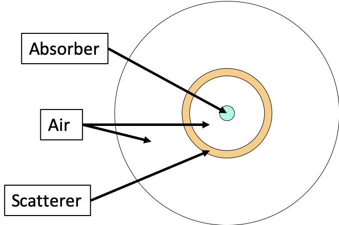
(a) Geometry for Example 1 in Section 7.1

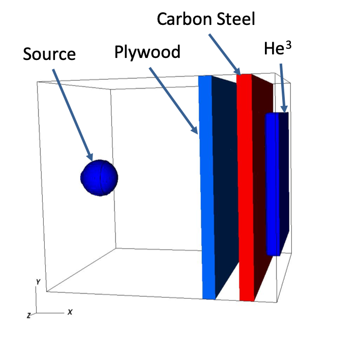
(b) Geometry for Example 2 in Section 7.2

Figure 2: Geometry description of numerical examples

7.1 Example 1: a symmetric case

The first example solves the Boltzmann particle transport equation on a 3D cartesian mesh. The mesh is $20\times 20\times 20$, resulting in $8,000$ spatial zones. There are eighty angular directions and seventeen energy groups. An absorber is located at the center and the second shell is scatterer as described in Figure 2a. The neutron source is $14.1$ $MeV$, which is in the 2nd energy group. The source is constant and the final simulation time step is at $T=40$ $nsec$ with a uniform time step $\Delta t=1$ $nsec$. As a result, there are $10,880,000$ degrees of freedom in space and $435,200,000$ degrees of freedom in space–time. The full order model simulation uses $8$ cores in RZTopaz and takes 22.5 seconds, resulting in the CPU time of around 3 minutes.

The space–time ROM is constructed, using $\epsilon_{\text{SVD}}=2\times 10^{-8}$ and $\epsilon_{\text{SV}}=10^{-14}$ for the basis size of $16$, whose reduction factor is around twenty-seven million. The ROM simulation uses $1$ core in RZTopaz. With the basis size of $16$, the relative error with respect to the full order model solution is less than $0.1\%$ as described in Figure 3(c). Figure 3(a) and (c) show the neutron flux distributions at the first and last time steps, respectively. The space–time ROM simulation with the basis size of $16$ takes $0.0055$ seconds, resulting in wall-clock time speed-up of $4,093.7$ and CPU time speed-up of $32,727.2$.

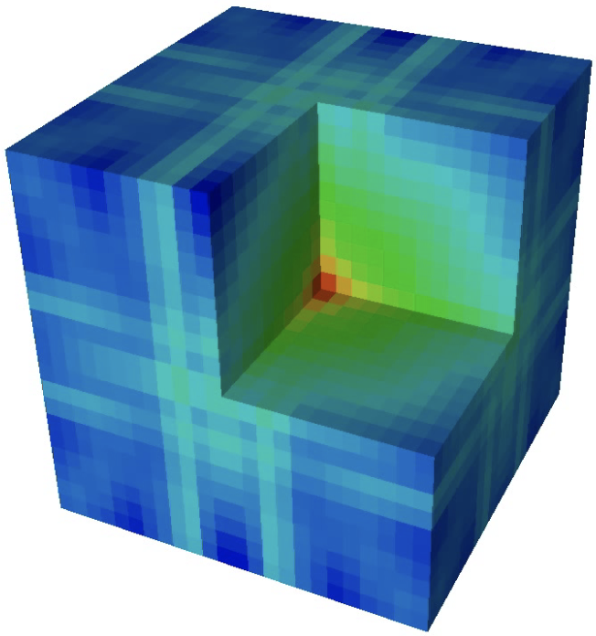
(a) Neutron flux at $t=0$ $nsec$

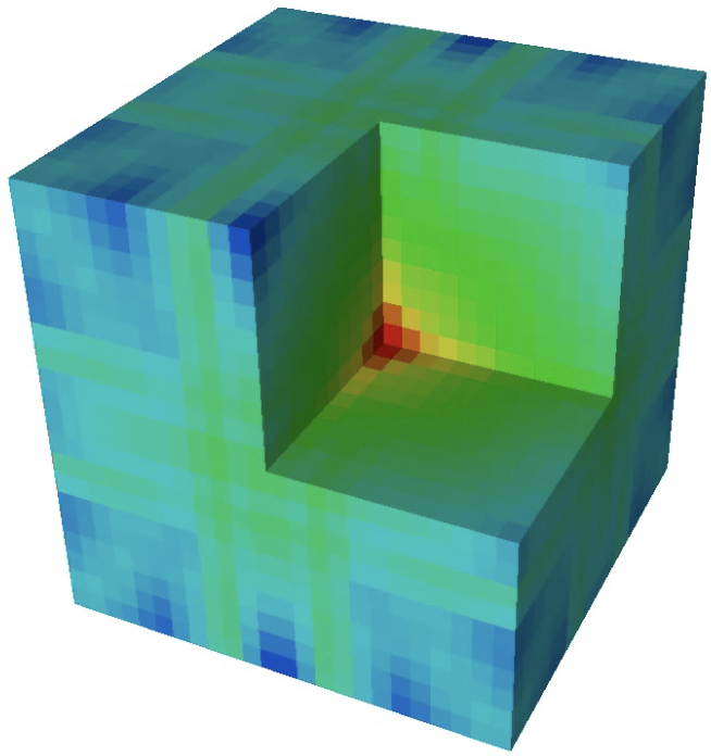
(b) Neutron flux at $t=40$ $nsec$

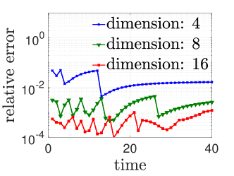
(c) relative error

Figure 3: Neutron flux and relative errors for the first problem

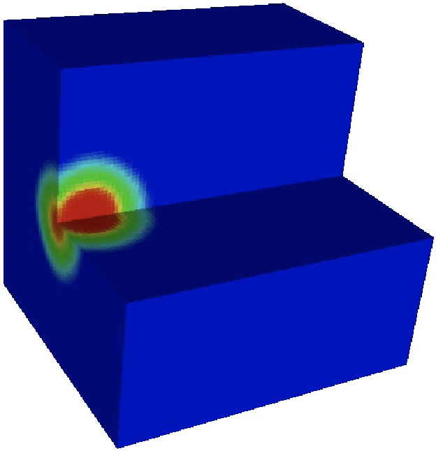
(a) Neutron flux at $t=0$ $nsec$

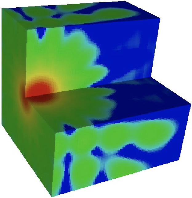
(b) Neutron flux at $t=30$ $nsec$

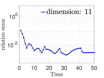
(c) relative error

Figure 4: Neutron flux and relative errors for the second problem, i.e., a truly 3D and larger-scale problem

7.2 Example 2: truly 3D case

The second example solves the Boltzmann particle transport equation on a different geometry, i.e., Figure 2b. This is truly 3D with more structure than the previous example. The neutron source is $14.1$ $MeV$, which is in the 2nd energy group. The source is constant and the final simulation time step is at $T=30$ $nsec$ with a uniform time step $\Delta t=0.2$ $nsec$. The mesh is $80\times 80\times 80$, resulting in $512,000$ spatial zones. There are eighty angular directions and seventeen energy groups. As a result, there are $696,320,000$ degrees of freedom in space and $104,448,000,000$ degrees of freedom in space and time. The full order model simulation uses $64$ cores in RZTopaz and takes 123.3 seconds, resulting in the CPU time of around 2.2 hours.

The space–time ROM is constructed, using $\epsilon_{\text{SVD}}=5\times 10^{-7}$ and $\epsilon_{\text{SV}}=10^{-14}$ for the basis size of $11$, whose reduction factor is around ten billion. The ROM simulation uses $1$ core in RZTopaz. With the basis size of $11$, the relative error with respect to the full order model solution is less than $1.0\%$ as described in Figure 4(c). Figure 4(a) and (c) show the neutron flux distributions at the first and last time steps, respectively. The space–time ROM simulation with the basis size of $11$ takes $0.00682$ seconds, resulting in wall-clock time speed-up of $7,891.2$ and CPU time speed-up of $1,157,067.4$.

8 Conclusion

Block structures in the space–time basis enable an efficient implementation of space–time reduced operators, which require small additional costs to the construction of the corresponding spatial ROM. Additionally, an incremental SVD is used to construct spatial and temporal bases in memory efficient way. As a result, the training cost of the space–time ROM is considerably reduced. Furthermore, because the space–time ROM achieves both space and time dimension reduction, considerably more reduction is accomplished than the spatial ROM, resulting in a great speed-up in online phase without losing much accuracy. It is demonstrated with Boltzmann transport problems where a reduction factor of twenty-seven million to ten billion and a CPU time speed-up of thirty-two thousand to one million were achieved by our space–time ROM. Finally, our space–time ROM is not limited to a space–time full order model formulation. It is amenable to any time integrators although the backward Euler time integrator is used as an illustration purpose in this paper.

Future works include applying the space–time ROM in the context of design optimization, uncertainty quantification, and inverse problems. Also, we will develop an efficient space–time ROM for nonlinear dynamical systems, such as TRT problems.

References

- [1] L. M. Adams. Subcell balance methods for radiative transfer on arbitrary grids. Transport Th. Statis. Phys., 26(4,5):385–431, 1997.
- [2] Amine Ammar, Béchir Mokdad, Francisco Chinesta, and Roland Keunings. A new family of solvers for some classes of multidimensional partial differential equations encountered in kinetic theory modeling of complex fluids. Journal of Non-Newtonian Fluid Mechanics, 139(3):153–176, 2006.
- [3] Amine Ammar, Béchir Mokdad, Francisco Chinesta, and Roland Keunings. A new family of solvers for some classes of multidimensional partial differential equations encountered in kinetic theory modelling of complex fluids: Part ii: Transient simulation using space-time separated representations. Journal of Non-Newtonian Fluid Mechanics, 144(2-3):98–121, 2007.
- [4] Zhaojun Bai. Krylov subspace techniques for reduced-order modeling of large-scale dynamical systems. Applied numerical mathematics, 43(1-2):9–44, 2002.
- [5] Patrick Behne, Jean Ragusa, and Jim Morel. Model-order reduction for sn radiation transport. In ANS International Conference on Mathematics and Computation (M&C). Portland, OR, USA, 2019.
- [6] Gal Berkooz, Philip Holmes, and John L Lumley. The proper orthogonal decomposition in the analysis of turbulent flows. Annual review of fluid mechanics, 25(1):539–575, 1993.
- [7] B. L. Bihari and P. N. Brown. A linear algebraic analysis of diffusion synthetic acceleration for the boltzmann transport equation ii: The simple corner balance method. SIAM J. Numer. Anal., 47(3):1782–1826, 2009.
- [8] BL Bihari and Peter N Brown. A linear algebraic analysis of diffusion synthetic acceleration for the boltzmann transport equation ii: The simple corner balance method. SIAM Journal on Numerical Analysis, 47(3):1782–1826, 2009.
- [9] Matthew Brand. Incremental singular value decomposition of uncertain data with missing values. In European Conference on Computer Vision, pages 707–720. Springer, 2002.
- [10] AG Buchan, CC Pain, F Fang, and IM Navon. A pod reduced-order model for eigenvalue problems with application to reactor physics. International Journal for Numerical Methods in Engineering, 95(12):1011–1032, 2013.
- [11] Andrew G Buchan, AA Calloo, Mark G Goffin, Steven Dargaville, Fangxin Fang, Christopher C Pain, and Ionel Michael Navon. A POD reduced order model for resolving angular direction in neutron/photon transport problems. Journal of Computational Physics, 296:138–157, 2015.
- [12] B. G. Carlson and K. D. Lathrop. Transport theory: The method of discrete ordinates. In H. Greenspan et al., editors, Computing Methods in Reactor Physics, pages 166–266. Gordon and Breach, New York, 1968.
- [13] Youngsoo Choi, William J. Arrighi, Dylan M. Copeland, Robert W. Anderson, Geoffrey M. Oxberry, and USDOE National Nuclear Security Administration. librom, 10 2019.
- [14] Youngsoo Choi and Kevin Carlberg. Space–time least-squares petrov–galerkin projection for nonlinear model reduction. SIAM Journal on Scientific Computing, 41(1):A26–A58, 2019.
- [15] Joseph Coale and Dmitriy Y. Anistratov. A reduced-order model for thermal radiative transfer problems based on multilevel quasidiffusion method. In ANS International Conference on Mathematics and Computation (M&C). Portland, OR, USA, 2019.
- [16] Kurt Dominesey and Wei Ji. Reduced-order modeling of neutron transport separated in space and angle via proper generalized decomposition. In ANS International Conference on Mathematics and Computation (M&C). Portland, OR, USA, 2019.
- [17] Kurt Dominesey and Wei Ji. A reduced-order neutron diffusion model separated in space and energy via proper generalized decomposition. In Transactions of the American Nuclear Society, volume 120, pages 457–460. Minneapolis, Minnesota, USA, 2019.
- [18] Hiba Fareed and John R Singler. Error analysis of an incremental pod algorithm for pde simulation data. arXiv preprint arXiv:1803.06313, 2018.
- [19] Serkan Gugercin, Athanasios C Antoulas, and Christopher Beattie. H_2 model reduction for large-scale linear dynamical systems. SIAM journal on matrix analysis and applications, 30(2):609–638, 2008.
- [20] Zachary K Hardy, Jim E Morel, and Cory Ahrens. Dynamic mode decomposition for subcritical metal systems. Nuclear Science and Engineering, pages 1–13, 2019.
- [21] Michael Hinze and Stefan Volkwein. Proper orthogonal decomposition surrogate models for nonlinear dynamical systems: Error estimates and suboptimal control. In Dimension reduction of large-scale systems, pages 261–306. Springer, 2005.
- [22] Harold Hotelling. Analysis of a complex of statistical variables into principal components. Journal of educational psychology, 24(6):417, 1933.
- [23] Karl Kunisch and Stefan Volkwein. Galerkin proper orthogonal decomposition methods for a general equation in fluid dynamics. SIAM Journal on Numerical analysis, 40(2):492–515, 2002.
- [24] E.Ẽ. Lewis and W.F̃. Miller. Computational Methods of Neutron Transport. American Nuclear Society, La Grange Park, IL, 1993.
- [25] R. L. Liboff. Introductory Quantum Mechanics. Holden-Day, Inc., San Francisco, 1980.
- [26] Michel Loeve. Probability Theory. D. Van Nostrand, New York, 1955.
- [27] Ryan G McClarren and Terry S Haut. Acceleration of source iteration using the dynamic mode decomposition. arXiv preprint arXiv:1812.05241, 2018.
- [28] Bruce Moore. Principal component analysis in linear systems: Controllability, observability, and model reduction. IEEE transactions on automatic control, 26(1):17–32, 1981.
- [29] C Mullis and RA Roberts. Synthesis of minimum roundoff noise fixed point digital filters. IEEE Transactions on Circuits and Systems, 23(9):551–562, 1976.
- [30] Zachary Prince and Jean Ragusa. Separated representation of spatial dimensions in neutron transport using the proper generalized decomposition. In ANS International Conference on Mathematics and Computation (M&C). Portland, OR, USA, 2019.
- [31] Zachary M Prince and Jean C Ragusa. Parametric uncertainty quantification using proper generalized decomposition applied to neutron diffusion. International Journal for Numerical Methods in Engineering, pages 1–23, 1993.
- [32] Richard L Reed and Jeremy A Roberts. An energy basis for response matrix methods based on the karhunen–loéve transform. Annals of Nuclear Energy, 78:70–80, 2015.
- [33] A. Sartori, D. Baroli, A. Cammi, D. Chiesa, L. Luzzi, R. Ponciroli, E. Previtali, M.E. Ricotti, G. Rozza, and M. Sisti. Comparison of a modal method and a proper orthogonal decomposition approach for multi-group time-dependent reactor spatial kinetics. Annals of Nuclear Energy, 71:217–229, 2014.
- [34] Peter J Schmid. Dynamic mode decomposition of numerical and experimental data. Journal of fluid mechanics, 656:5–28, 2010.
- [35] Lawrence Sirovich. Turbulence and the dynamics of coherent structures. i. coherent structures. Quarterly of applied mathematics, 45(3):561–571, 1987.
- [36] S Kelbij Star, Francesco Belloni, Gert Van den Eynde, and Joris Degroote. Pod-identification reduced order model of linear transport equations for control purposes. International Journal for Numerical Methods in Fluids, 90(8):375–388, 2019.
- [37] Jonathan H Tu, Clarence W Rowley, Dirk M Luchtenburg, Steven L Brunton, and J Nathan Kutz. On dynamic mode decomposition: theory and applications. arXiv preprint arXiv:1312.0041, 2013.
- [38] Karsten Urban and Anthony Patera. An improved error bound for reduced basis approximation of linear parabolic problems. Mathematics of Computation, 83(288):1599–1615, 2014.
- [39] Frank Wols. Transient analyses of accelerator driven systems using modal expansion techniques. PhD thesis, Delft University of Technology, 2010.
- [40] Masayuki Yano. A space-time petrov–galerkin certified reduced basis method: Application to the boussinesq equations. SIAM Journal on Scientific Computing, 36(1):A232–A266, 2014.
- [41] Masayuki Yano, Anthony T Patera, and Karsten Urban. A space-time hp-interpolation-based certified reduced basis method for burgers’ equation. Mathematical Models and Methods in Applied Sciences, 24(09):1903–1935, 2014.