On fractional Lévy processes: tempering, sample path properties and stochastic integration

Abstract

We define two new classes of stochastic processes, called tempered fractional Lévy process of the first and second kinds (TFLP and TFLP II, respectively). TFLP and TFLP II make up very broad finite-variance, generally non-Gaussian families of transient anomalous diffusion models that are constructed by exponentially tempering the power law kernel in the moving average representation of a fractional Lévy process. Accordingly, the increment processes of TFLP and TFLP II display semi-long range dependence. We establish the sample path properties of TFLP and TFLP II. We further use a flexible framework of tempered fractional derivatives and integrals to develop the theory of stochastic integration with respect to TFLP and TFLP II, which may not be semimartingales depending on the value of the memory parameter and choice of marginal distribution.

1 Introduction

In this paper, we define two new classes of stochastic processes, called tempered fractional Lévy processes of the first and second kinds (TFLP and TFLP II, respectively). TFLP and TFLP II make up very broad finite-variance, generally non-Gaussian transient anomalous diffusion models, i.e., their second order properties qualitatively change over time. They are constructed by exponentially tempering the power law kernel in the moving average representation of a fractional Lévy process (FLP). In particular, their increment processes exhibit semi-long range dependence (semi-LRD) in the sense of [42], namely, their autocovariance functions decay hyperbolically over small lags and exponentially fast over large lags (see (1.2)). We establish the sample path regularity of TFLPs. Turning to stochastic analysis, we use a flexible framework of tempered fractional derivatives and integrals to develop the theory of stochastic integration with respect to TFLP and TFLP II, which may not be semimartingales depending on the value of the memory parameter and choice of marginal distribution.

Fractional, or non-Markovian, stochastic processes naturally emerge in many fields of science, technology and engineering (see, e.g., [61, 28, 37, 46, 60, 97]). They provide the mathematical framework for what is called scale-free analysis [61, 36, 102]. Rather than focusing on the detection of a small number of characteristic scales, in scale-free analysis it is assumed that the phenomenological dynamics are driven by a large continuum of time scales usually related by means of a power law. A cornerstone class of scale invariant processes is fractional Brownian motion (FBM), i.e., the only Gaussian, self-similar, stationary increment process [34, 77]. The literature on fractional processes is now voluminous; see, e.g., [18, 33, 44, 71, 98, 99, 88, 2, 29].

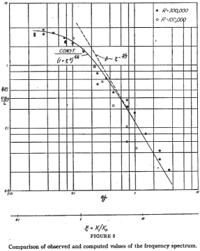
Figure 1: The Von Kármán spectral density (curved line) versus Kolmogorov’s 5/3 law (straight line). Kolmogorov’s classical theory [52, 53, 40, 92] posits that the energy spectrum in the inertial range is universal and given by the frequency domain power law $\omega^{-5/3}$. However, in the production (low frequency) range, turbulence is not universal, which may lead to transient behavior. In the Von Kármán model of continuous wind gusts [101, 31, 75, 14, 47, 73], the framework favored by the U.S. Department of Defense in aircraft design, the spectral density is proportional to $(\lambda^{2}+\omega^{2})^{-5/6}$ with $\lambda=1$ (see [30, 72, 57, 13, 31]). The tempering parameter $\lambda$ dampens down, in the low frequency limit, the power law behavior universally valid for the inertial range. The spectral density of tempered fractional Lévy noise $I\!I$, the increment process of TFLP $I\!I$, is of the Von Kármán type (see Proposition 2.13).

In many empirical settings, power law behavior is expected to hold only within a range of scales, out of which the observed dynamics qualitatively change, possibly to different power law behavior or simply non-fractional stationarity. In anomalous diffusion modeling, this is typically reflected in the behavior of the so-named mean squared displacement (MSD)

$$\mathbb{E}X^{2}(t)\approx Ct^{\vartheta},\quad C,\vartheta\geq 0,$$ (1.1)

of the particle position $X(t)$ over a time interval $T\ni t$, where the instances $\vartheta=1$ and $\vartheta\neq 1$ correspond to classical and anomalous behavior, respectively (e.g., [69, 54, 94, 32, 45, 108]). In the physics literature, a particle is said to undergo transient anomalous diffusion when the value of the exponent $\vartheta$ in (1.1) changes over different time intervals (e.g., [78, 95, 1, 89, 103, 24, 58, 25]). Transience may appear in several contexts such as in nanobiophysics [91, 70] and particle dispersion [100, 104]. It also arises as a consequence of accounting for the energy spectrum of turbulence in the low frequency range, leading to the so-named Davenport– [20] or Von Kármán–type spectra (see Figure 1).

Tempered FBM of the first and second kinds (TFBM [64] and TFBM $I\!I$ [85], respectively) are transient anomalous diffusion models. For TFBM, the MSD in (1.1) goes from $\vartheta>0$ over small time scales to $\vartheta=0$ over large scales, as in geophysical flows [68, 66]. By contrast, for TFBM $I\!I$, it shifts from anomalous over small scales to regular ($\vartheta=1$) over large scales, as in viscoelastic diffusion (cf. [39, 38, 105]). Accordingly, the autocovariance functions $\gamma$ of the increments of both TFBM and TFBM $I\!I$ have the related property of semi-LRD, i.e.,

$$\gamma(h)\sim C\frac{|h|^{\delta}}{e^{\lambda|h|}},\quad\lambda>0,\quad\delta>-\frac{3}{2},\quad|h|\rightarrow\infty,$$ (1.2)

where $\lambda>0$ is called the tempering parameter (see also Remark 2.4 on the related literature on Lévy semistationary processes). Moreover, like FBM vis-à-vis the Kolmogorov spectrum in the inertial range, TFBM $I\!I$ [64, 65] is a Gaussian model that displays a von Kármán–type spectrum. Due to their appeal in applications, TFBMs have recently attracted considerable research efforts [107, 24]. In [20, 21], wavelets are used in the construction of the first statistical method for TFBM as a model of geophysical flow turbulence. Nevertheless, there is abundant phenomenological evidence of non-Gaussian behavior, especially in terms of tail distributions. This is true, for example, for the velocity and velocity derivative processes in wind turbulence [4, 5, 7, 8, 9, 93] or returns to financial assets [6]; see also Figure 2. Accordingly, many authors have developed several other classes of tempered non-Gaussian stochastic processes such as tempered fractional stable or tempered Hermite processes [85, 84], and tempered stable processes [82, 1, 19, 41, 83, 50, 55].

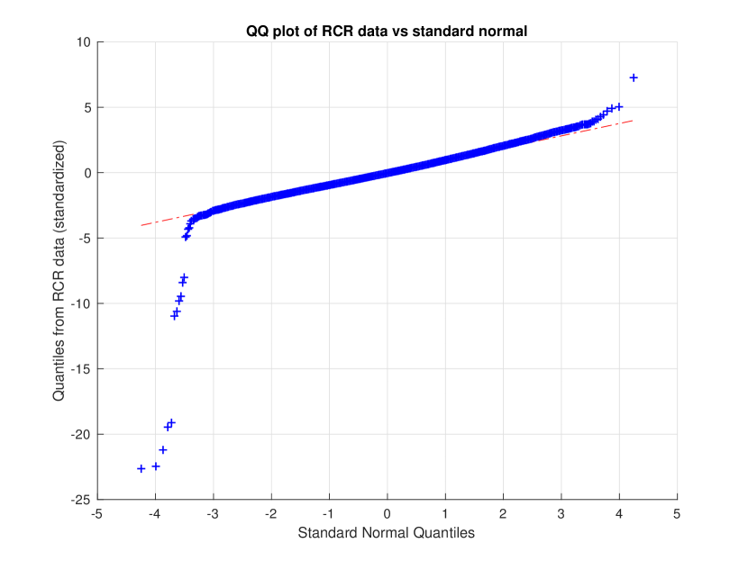
Figure 2: Non-Gaussianity in river flow turbulence. Data on turbulent supercritical flow in the Red Cedar River, a fourth-order stream in Michigan, USA, was collected and kindly provided by Prof. Mantha S. Phanikumar, from Michigan State University. The measurements ($n=46080$ points) were made at a sampling rate of 50 Hz using a 16 MHz Sontek Micro-ADV (Acoustic Doppler Velocimeter) on May 26, 2014. The data is modeled in [66] in the Fourier and in [21, 20] in the wavelet domains. The qq–plot, shown above, further reveals the conspicuous non-Gaussianity of the sample tails.

The family of fractional Lévy processes (e.g., [15, 22, 62, 56, 17]) has become popular in physical modeling since it provides a second order non-Gaussian framework displaying fractional covariance structure [11, 96, 59, 109, 106]. In this paper, we construct the classes of TFLP and TFLP $I\!I$, which are families of tempered fractional processes with finite-variance, infinitely divisible finite-dimensional distributions. While FLP (including FBM) is only well-defined for memory parameter values $d\in(-1/2,1/2)$ [35, 62], TFLPs are well-defined for every $d>-1/2$ due to the tempering effect of the exponential function in their kernels. We establish their second order and sample path regularity properties (see Propositions 2.3, 2.7, 2.9 and 2.13 and Theorems 2.6 and 2.12). In our analysis, continuous modifications of TFLP and TFLP II can also be obtained, under conditions, by means of improper Riemann integral representations (Propositions 2.5 and 2.11; see also Bender et al. [16] for related results in a general martingale-driven framework). In particular, our results show that TFLP and TFLP $I\!I$ can be viewed as non-Gaussian transient anomalous diffusion models whose second order properties generalize those of TFBM and TFBM $I\!I$, respectively (see also Example 2.15 and Figures 3, 4 on the effect of non-Gaussian noise distributions on sample path behavior).

Physical models of transient phenomena are often based on Langevin-type stochastic differential equations; see, for example, [70] on the transient MSD of solutions to TFBM-driven Langevin equations, and [27] on turbulence modeling based on regularized colored noise. In this paper, we approach stochastic differential systems from the dual perspective of integration. For the purpose of stochastic analysis, TFLPs are finite variation processes when $d>1/2$ (see Proposition 3.1), and hence integration with respect to these processes can be defined pathwise in the usual Stieltjes manner. However, like FLP, when $-1/2<d<1/2$ TFLPs may not be finite variation processes, or even semimartingales (Proposition 2.14 and Remark 2.16). For this parameter range, we construct the theory of Wiener-like integrals with respect to these processes. Our approach follows the seminal work [76] for FBM, later extended in [65] to TFBM. Whereas the integration theory with respect to FBM draws upon classical fractional derivatives [67, 74, 87], we put forward a framework for TFLPs based on tempered fractional derivatives [23, 1]. Tempering produces a more tractable mathematical object, and can be made arbitrarily light, so that the resulting operators approximate the fractional derivative to any desired degree of accuracy over compact intervals.

We focus on integration with respect to TFLP II (denoted $S^{I\!I}_{d,\lambda}$, $\lambda>0$), since the claims for TFLP are analogous to those for TFBM (see Remark 3.12). Our construction follows from characterizing the natural inner product spaces of integrands ${\mathcal{A}}_{1}$ and ${\mathcal{A}}_{2}$ (see (3.16) and (3.22)), which are associated with the memory parameter ranges $-1/2<d<0$ and $d>0$, respectively. In particular, we show that, for TFLP II, the phenomenon revealed in [76] for FBM resurfaces in the context of tempered fractional Lévy-type stochastic integration. In other words, for $-1/2<d<0$, ${\mathcal{A}}_{1}$ and the space of stochastic integrals $\overline{\rm Sp}(S^{I\!I}_{d,\lambda})$ are isometric. As a consequence, every random variable in $\overline{\rm Sp}(S^{I\!I}_{d,\lambda})$ with $-1/2<d<0$ can be written as an integral of a single deterministic function with respect to the stochastic process $S^{I\!I}_{d,\lambda}$ (see Theorems 3.9 and 3.11). However, for $d>0$, our results show that ${\mathcal{A}}_{2}$ is isometric only to a subspace of $\overline{\rm Sp}(S^{I\!I}_{d,\lambda})$ (see Theorems 3.5 and 3.8).

The paper is organized as follows. Section 2 contains the definitions and fundamental properties of TFLPs, where Sections 2.1 and 2.2 pertain to TFLP and TFLP II, respectively. In Section 3, we first show that TFLP and TFLP $I\!I$ are semimartingales for $d>1/2$ and then construct the theory of stochastic integration with respect to these processes for $-1/2<d<1/2$. In Section 4, we sum up the conclusions and discuss open problems as well as future research directions. All proofs can be found in the Appendix.

2 Moving average representation

Recall that a Lévy process is a stochastically continuous process with stationary and independent increments that starts at zero and has càdlàg sample paths a.s.  [90]. Throughout this paper, Lévy noise plays the role that Brownian noise plays in a Gaussian framework. So, let $L=\{L(t)\}_{t\in\mathbb{R}}$ be a two-sided Lévy process constructed by taking two independent copies $L_{1}=\{L_{1}(t)\}_{t\geq 0}$ and $L_{2}=\{L_{2}(t)\}_{t\geq 0}$ of a Lévy process and by setting

$$L(t):=L_{1}(t){\bf 1}_{[0,\infty)}(t)-L_{2}((-t)-){\bf 1}_{(-\infty,0)}(t).$$ (2.1)

Hereinafter, we assume $L$ as in (2.1) satisfies the following condition.

Condition $L$: The Lévy process $L$ in (2.1) is centered ($\mathbb{E}[L(1)]=0$) and contains no Brownian component. The distribution of $L$ is uniquely determined by the characteristic function (ch.f.) $\mathbb{E}[\exp{i\theta L(t)}]=\exp\{t\psi(\theta)\}$ for $t\geq 0$, where

$$\psi(\theta)=\int_{\mathbb{R}}(e^{i\theta x}-1-i\theta x)\nu(dx),\quad\quad\theta\in\mathbb{R}.$$ (2.2)

In (2.2), $\nu(dx)$ is called the Lévy measure of $L$, i.e.,

$$\nu(\{0\})=0,\qquad\int_{\mathbb{R}}(|x|^{2}\wedge 1)\nu(dx)<\infty.$$

Moreover, $\nu(dx)$ is assumed to be such that $\int_{|x|>1}x^{2}\nu(dx)<\infty$, i.e., $\mathbb{E}[(L(t))^{2}]=t\mathbb{E}[(L(1))^{2}]=t\int_{\mathbb{R}}|x|^{2}\nu(dx)<\infty$ for all $t\in\mathbb{R}$.

We recall the following classical result for later reference. It provides the conditions for the existence, in the $L^{2}(\Omega)$ sense, of Wiener-like stochastic integrals with respect to Lévy noise.

Proposition 2.1

[80, 51] Let $f:\mathbb{R}\times\mathbb{R}\to\mathbb{R}$ be a measurable function. Let $L$ be a Lévy process such that $\mathbb{E}[L(1)]=0$ and $\mathbb{E}[(L(1))^{2}]<\infty$. For $t\in\mathbb{R}$, let $f_{t}(\cdot)\in L^{2}(\mathbb{R})$. Then, the stochastic integral $S(t):=\int_{\mathbb{R}}f_{t}(u)dL(u)$ exists in the $L^{2}(\Omega)$ sense for any $t\in\mathbb{R}$. Furthermore, for $t\in\mathbb{R}$, $\mathbb{E}[S(t)]=0$. The isometry

$$\mathbb{E}[(S(t))^{2}]=\mathbb{E}[(L(1))^{2}]\|f_{t}\|^{2}_{L^{2}(\mathbb{R})},\quad t\in\mathbb{R},$$ (2.3)

also holds, as well as the relation

$$\widetilde{\Gamma}(s,t)={\rm cov}(S(s),S(t))=\mathbb{E}[(L(1))^{2}]\int_{\mathbb{R}}f_{s}(u)f_{t}(u)du,\quad s,t\in\mathbb{R},$$ (2.4)

Moreover, the ch.f. of $S(t_{1}),\ldots,S(t_{m})$ for $-\infty<t_{1}<\ldots<t_{m}<\infty$ is given by

$$\mathbb{E}\Big{[}\exp\Big{\{}\sum_{j=1}^{m}i\theta_{j}S(t_{j})\Big{\}}\Big{]}=\exp\Big{\{}\int_{\mathbb{R}}\psi\Big{(}\sum_{j=1}^{m}\theta_{j}f_{t_{j}}(s)\Big{)}ds\Big{\}}$$ (2.5)

for $\theta_{j}\in\mathbb{R},j=1,2,\ldots,m$, where $\psi$ is given by (2.2).

2.1 Tempered fractional Lévy processes of the first kind

In this section, we introduce and study tempered fractional Lévy process of the first kind. We start with its definition.

Definition 2.2

Let $L=\{L(t)\}_{t\in\mathbb{R}}$ be the two-sided Lévy process (2.1). Consider the function $(x)_{+}=xI(x>0)$ and set the convention $0^{0}=0$. Consider the function $g^{I}_{d,\lambda,t}:\mathbb{R}\rightarrow\mathbb{R}$ given by

$$g^{I}_{d,\lambda,t}(x):=e^{-\lambda(t-x)_{+}}{(t-x)_{+}^{d}}-e^{-\lambda(-x)_{+}}{(-x)_{+}^{d}}.$$

For any $d>-\frac{1}{2}$ and $\lambda>0$, the stochastic process

$$S^{I}_{d,\lambda}(t):=\frac{1}{\Gamma(1+d)}\int_{\mathbb{R}}g^{I}_{d,\lambda,t}(x)dL(x),\quad t\in\mathbb{R},$$ (2.6)

is called a tempered fractional Lévy process of the first kind (TFLP).

The kernel function $g^{I}_{d,\lambda,t}(x)$ is square integrable over $\mathbb{R}$. Hence, by Proposition 2.1, the stochastic integral in (2.6) exists in the $L^{2}(\Omega)$ sense for any $t\in\mathbb{R}$.

The class of stochastic processes given by Definition 2.2 is closely related to a number of other frameworks. When $-\frac{1}{2}<d<\frac{1}{2}$ and tempering is eliminated ($\lambda=0$), the expression on the right-hand side of (2.6) is the classical FLP. If $d=0$ (and $\lambda>0$), then $S^{I}_{0,\lambda}(t)$ is called a Lévy Ornstein-Uhlenbeck (OU) process ([90], Section 3.17). If $dL(x)$ in (2.6) is replaced with a Gaussian random measure, the resulting process is a TFBM.

Hereinafter, for $S^{I}_{d,\lambda}$ we assume $d\neq 0$ (and $\lambda>0$) unless otherwise stated. Note also that, for any $s,t\in\mathbb{R}$, the integrand (2.2) satisfies $g^{I}_{d,\lambda,s+t}(s+x)-g^{I}_{d,\lambda,s}(s+x)=g^{I}_{d,\lambda,t}(x)$, and hence one can show that TFLP has stationary increments. In the next proposition, we provide the covariance structure of TFLP.

Proposition 2.3

A TFLP $S^{I}_{d,\lambda}$ (see (2.6)) has the covariance function

$${\rm Cov}\left[S^{I}_{d,\lambda}(t),S^{I}_{d,\lambda}(s)\right]=\frac{\mathbb{E}[(L(1))^{2}]}{2\Gamma(1+d)^{2}}\Big{\{}|t|^{1+2d}C^{2}_{d,\lambda,|t|}+|s|^{1+2d}C^{2}_{d,\lambda,|s|}-|t-s|^{1+2d}C^{2}_{d,\lambda,|t-s|}\Big{\}}$$ (2.7)

for any $s,t\in\mathbb{R}$. In (2.7),

$$C^{2}_{d,\lambda,|t|}=\frac{2\Gamma(1+2d)}{(2\lambda|t|)^{1+2d}}-\frac{2\Gamma(1+d)}{\sqrt{\pi}}\Big{(}\frac{1}{2\lambda|t|}\Big{)}^{\frac{1}{2}+d}K_{\frac{1}{2}+d}(\lambda|t|),$$ (2.8)

for $t\neq 0$, and we define $C_{d,\lambda,0}^{2}=0$. In (2.8), $K_{\nu}(z)$ is the modified Bessel function of the second kind, which is given by

$$K_{\nu}(z)=\int^{\infty}_{0}e^{-z(\frac{e^{-t}+e^{t}}{2})}\frac{e^{-\nu t}+e^{\nu t}}{2}dt,\quad z>0,\quad\nu\in\mathbb{R}.$$

Moreover,

$$\lim_{t\to\infty}{\rm Var}\big{[}S^{I}_{d,\lambda}(t)\big{]}=\frac{2\mathbb{E}(L(1)^{2})\Gamma(1+2d)}{\Gamma(1+d)^{2}(2\lambda)^{1+2d}}.$$ (2.9)

It is well known that the variance of FLP is divergent [62]. Remarkably, expression (2.9) shows that the variance of TFLP stays finite in the large scale limit (cf. [20], Proposition A.1).

Remark 2.4

Let $L=\{L(t)\}_{t\in\mathbb{R}}$ be the two-sided Lévy process (2.1). Then, a Lévy semistationary process (LSS; see [3, 10]) is defined by the stochastic integral representation

$$Y(t)=\mu+\int_{-\infty}^{t}g(t-s)\sigma(s)dL(s)+\int_{-\infty}^{t}q(t-s)a(s)ds,$$ (2.10)

where $\sigma$ and $a$ are stochastic processes, and $g$ and $q$ are deterministic kernels with $g(t)=h(t)=0$ for $t\leq 0$. Although LSS instances associated with gamma kernels ($g(x)=x^{d-1}e^{-\lambda x}$) and TFLP both display a tempering component, the two processes are generally quite different. In particular, the former may be stationary, while the latter is always nonstationary.

In the next proposition, we establish a stochastic integral representation of TFLP as an improper Riemann integral for the parameter range $d>0$. The result is then used in part $(a)$ of the subsequent theorem to construct a Hölder–continuous modification of TFLP.

Proposition 2.5

Let $S^{I}_{d,\lambda}=\{S^{I}_{d,\lambda}(t)\}_{t\in\mathbb{R}}$ be a TFLP (see (2.6)) with $d>0$. Then, for all $t\in\mathbb{R}$, there exists a modification of $S^{I}_{d,\lambda}(t)$ which is equal to the improper Riemann integral

$$\begin{split}S^{I}_{d,\lambda}(t)&=\frac{1}{\Gamma(d)}\int_{\mathbb{R}}\Big{(}e^{-\lambda(t-x)_{+}}{(t-x)_{+}^{d-1}}-e^{-\lambda(-x)_{+}}{(-x)_{+}^{d-1}}\Big{)}\ L(x)\ dx\\ &\qquad\qquad-\frac{\lambda}{\Gamma(d+1)}\int_{\mathbb{R}}\Big{(}e^{-\lambda(t-x)_{+}}(t-x)_{+}^{d}-e^{-\lambda(-x)_{+}}(-x)_{+}^{d}\Big{)}\ L(x)\ dx.\end{split}$$ (2.11)

In particular, the process (2.11) is continuous in $t$.

The following theorem is our main result on the sample path properties of TFLP. Note that the statement in $(a)$ is slightly stronger than the one usually obtained in the framework of the Kolmogorov-$\breve{\textnormal{C}}$entsov criterion.

Theorem 2.6

Let $S^{I}_{d,\lambda}=\{S^{I}_{d,\lambda}(t)\}_{t\in\mathbb{R}}$ be a TFLP (see (2.6)).

• If $0<d\leq\frac{1}{2}$, then there exists a locally $d$-Hölder continuous modification of $S^{I}_{d,\lambda}$. That is, for $T>0$,

  $$\mathbb{P}\Bigg{[}\omega:\sup_{0<|s-t|<k_{T}(\omega),|s|\leq T,|t|\leq T}\Big{(}\frac{|S^{I}_{d,\lambda}(t)-S^{I}_{d,\lambda}(s)|}{|s-t|^{d}}\Big{)}\leq C\Bigg{]}=1,$$ (2.12)

  where $k_{T}(\omega)$ is an almost surely positive random variable and $C>0$.

• If $-\frac{1}{2}<d<0$ and $L$ has symmetric finite-dimensional distributions, then $S^{I}_{d,\lambda}$ has discontinuous and unbounded sample paths with positive probability.

Next, we turn to the increment process of TFLP. Starting from a TFLP $S^{I}_{d,\lambda}$, the stationary process tempered fractional Lévy noise of the first kind (TFLN) is naturally defined as

$$X^{I}_{d,\lambda}(t):=S^{I}_{d,\lambda}(t+1)-S^{I}_{d,\lambda}(t),\quad t\in\mathbb{R}.$$ (2.13)

It follows readily from (2.6) that TFLN has the moving average representation

$$X^{I}_{d,\lambda}(t)=\frac{1}{\Gamma(d+1)}\int_{\mathbb{R}}\big{[}e^{-\lambda(t+1-x)_{+}}(t+1-x)_{+}^{d}-e^{-\lambda(t-x)_{+}}(t-x)_{+}^{d}\big{]}\ dL(x).$$ (2.14)

In the following proposition, we characterize the behavior of the covariance of TFLN over large lags. In particular, TFLN is semi-LRD in the sense of (1.2) with $\delta=d>-1/2$.

Proposition 2.7

Let $X^{I}_{d,\lambda}=\{X^{I}_{d,\lambda}(t)\}_{t\in\mathbb{R}}$ be a TFLN (see (2.14)). Let $\gamma^{I}(h)=\mathbb{E}[X^{I}_{d,\lambda}(0)X^{I}_{d,\lambda}(h)]$ be its covariance function and let $h^{I}(\omega)$ be its spectral density. Then,

• as $h\to\infty$,

  $$\gamma^{I}(h)\sim Ce^{-\lambda h}h^{d},$$ (2.15)

  where $C=C(d,\lambda)=-\frac{\mathbb{E}[L(1)^{2}]\lambda^{2}}{\Gamma(d+1)(2\lambda)^{d+1}}$;

• for $\omega\in\mathbb{R}$,

  $$h^{I}(\omega)=\frac{1}{2\pi}\frac{(1-\cos{\omega})}{(\lambda^{2}+\omega^{2})^{d+1}}.$$ (2.16)

2.2 Tempered fractional Lévy processes of the second kind

In this section, we introduce and study tempered fractional Lévy process of the second kind. We start with its definition.

Definition 2.8

Let $L=\{L(t)\}_{t\in\mathbb{R}}$ be the two-sided Lévy process (2.1) and consider the function $g^{I\!I}_{d,\lambda,t}:\mathbb{R}\to\mathbb{R}$ given by

$$g^{I\!I}_{d,\lambda,t}(y)=(t-y)_{+}^{d}\ e^{-\lambda(t-y)_{+}}-(-y)_{+}^{d}\ e^{-\lambda(-y)_{+}}+\lambda\int_{0}^{t}(s-y)_{+}^{d}\ e^{-\lambda(s-y)_{+}}\ ds.$$

For any $d>-\frac{1}{2}$ and $\lambda>0$, the stochastic process

$$S^{I\!I}_{d,\lambda}(t):=\frac{1}{\Gamma(d+1)}\int_{\mathbb{R}}g^{I\!I}_{d,\lambda,t}(y)\ dL(y),\quad t\in\mathbb{R},$$ (2.17)

is called a tempered fractional Lévy process of the second kind (TFLP II).

By Proposition 2.1, $S^{I\!I}_{d,\lambda}(t)$ is well defined in the $L^{2}(\Omega)$ sense for any $t\in\mathbb{R}$, since $g^{I\!I}_{d,\lambda,t}(y)$ is square integrable (see Lemma A.1).

As with (2.6), the class of stochastic processes given by (2.17) is closely related to other frameworks. When $-\frac{1}{2}<d<\frac{1}{2}$ and tempering is eliminated ($\lambda=0$), the process $S^{I\!I}_{d,0}(t)$ also reduces to FLP. If $dL(x)$ in (2.17) is replaced with a Gaussian random measure, the resulting process is a TFBM $I\!I$.

Hereinafter, for $S^{I\!I}_{d,\lambda}$ we assume $d\neq 0$ (and $\lambda>0$), unless otherwise stated.

In the following proposition, we express the covariance function $\mathbb{E}[S^{I\!I}_{d,\lambda}(t)S^{I\!I}_{d,\lambda}(s)]$ of TFLP $I\!I$ when $d>0$.

Proposition 2.9

For $d>0$, a TFLP $I\!I$ (see (2.17)) has covariance function

$${\rm Cov}\left[S^{I\!I}_{d,\lambda}(t),S^{I\!I}_{d,\lambda}(s)\right]=\frac{\mathbb{E}[L(1)^{2}]}{\sqrt{\pi}\Gamma(d)(2\lambda)^{d-\frac{1}{2}}}\int_{0}^{t}\int_{0}^{s}|u-v|^{d-\frac{1}{2}}K_{d-\frac{1}{2}}(\lambda|u-v|)dv\ du$$ (2.18)

for any $s,t\in\mathbb{R}$.

Remark 2.10

In the parameter range $-1/2<d<0$, the covariance of TFLP $I\!I$ can be found by first developing $\mathbb{E}[(S^{I\!I}_{d,\lambda}(t))^{2}]$ via the isometry property (2.3), and then applying the elementary formula $ab=\frac{1}{2}(a^{2}+b^{2}-(a-b)^{2})$ as well as the stationary increments property. However, the final formula for $\mathbb{E}[(S^{I\!I}_{d,\lambda}(t))^{2}]$ involves several integral expressions, and consequently so does the formula for $\mathbb{E}[S^{I\!I}_{d,\lambda}(t)S^{I\!I}_{d,\lambda}(s)]$. For brevity and clarity of exposition, we opt for not including it here.

The next proposition is the analog for TFLP $I\!I$ of Proposition 2.5. It shows that TFLP $I\!I$ has a modification that can be written as an improper Riemann integral.

Proposition 2.11

Let $S^{I\!I}_{d,\lambda}=\{S^{I\!I}_{d,\lambda}(t)\}_{t\in\mathbb{R}}$ be a TFLP $I\!I$ (see (2.17)) with $d>0$. Then, for all $t\in\mathbb{R}$, there exists a modification of $S^{I\!I}_{d,\lambda}(t)$ which is equal to the improper Riemann integral

$$\begin{split}S^{I\!I}_{d,\lambda}(t)&=\frac{1}{d\Gamma(d-1)}\int_{\mathbb{R}}\int_{0}^{t}e^{-\lambda(s-x)_{+}}(s-x)_{+}^{d-2}dsL(x)dx\\ &-\frac{\lambda}{\Gamma(d-1)}\int_{\mathbb{R}}\int_{0}^{t}e^{-\lambda(s-x)_{+}}(s-x)_{+}^{d-1}dsL(x)dx.\end{split}$$ (2.19)

In particular, the process (2.19) is continuous in $t$.

The following theorem is our main result on the sample path properties of TFLP $I\!I$.

Theorem 2.12

Let $S^{I\!I}_{d,\lambda}=\{S^{I\!I}_{d,\lambda}(t)\}_{t\in\mathbb{R}}$ be a TFLP $I\!I$ (see (2.17)).

• If $0<d\leq\frac{1}{2}$, then for every $0<\gamma<d$, there exists a locally $\gamma$-Hölder continuous modification of $S^{I\!I}_{d,\lambda}$. That is, for $T>0$,

  $$\mathbb{P}\Bigg{[}\omega:\sup_{0<|s-t|<k_{T}(\omega),|s|\leq T,|t|\leq T}\Big{(}\frac{|S^{I\!I}_{d,\lambda}(t)-S^{I\!I}_{d,\lambda}(s)|}{|s-t|^{\gamma}}\Big{)}\leq C\Bigg{]}=1,$$ (2.20)

  where $k_{T}(\omega)$ is an almost surely positive random variable and $C>0$.

• If $-\frac{1}{2}<d<0$ and $L$ has symmetric finite-dimensional distributions, then $S^{I\!I}_{d,\lambda}$ has discontinuous and unbounded sample paths with positive probability.

Next, we turn to the increment process of TFLP $I\!I$. Starting from a TFLP $I\!I$ $S^{I\!I}_{d,\lambda}$, the stationary process tempered fractional Lévy noise of the second kind (TFLN $I\!I$) is naturally defined as

$$X^{I\!I}_{d,\lambda}(t)=S^{I\!I}_{d,\lambda}(t+1)-S^{I\!I}_{d,\lambda}(t),\quad t\in\mathbb{R}.$$ (2.21)

It follows from (2.17) that TFLN $I\!I$ has moving average representation

$$X^{I\!I}_{d,\lambda}(t)=\frac{1}{\Gamma(d)}\int_{\mathbb{R}}\int_{t}^{t+1}(s-y)_{+}^{d}e^{-\lambda(s-y)_{+}}\ ds\ dL(y).$$ (2.22)

The following proposition describes the behavior of the covariance structure of TFLN $I\!I$ over large lags. In particular, the proposition shows that TFLN$I\!I$ is semi-LRD in the sense of (1.2) with $\delta=d-1>-3/2$. In the Fourier domain, it shows that the spectral density is of the Von Kármán type (cf. Figure 1). In the statement of the proposition, we make use of the following notation: given two real-valued functions $f(t)$, $g(t)$ on $\mathbb{R}$, we write $f(t)\asymp g(t)$ if $C_{1}\leq|{f(t)}/{g(t)}|\leq C_{2}$ for all $t>0$ sufficiently large, for some $0<C_{1}<C_{2}<\infty$.

Proposition 2.13

Let $X^{I\!I}_{d,\lambda}=\{X^{I\!I}_{d,\lambda}(t)\}_{t\in\mathbb{R}}$ be a TFLN $I\!I$ (see (2.21)). Let $\gamma^{I\!I}(h)=\mathbb{E}[X^{I\!I}_{d,\lambda}(0)X^{I\!I}_{d,\lambda}(h)]$, $h\in\mathbb{R}$, be its covariance function, and let $\{h^{I\!I}(\omega)\}_{\omega\in\mathbb{R}}$ be its spectral density. Then,

• as $h\to\infty$,

  $$\gamma^{I\!I}(h)\asymp e^{-\lambda h}h^{d-1};$$ (2.23)

• for $\omega\in\mathbb{R}$,

  $$h^{I\!I}(\omega)=\frac{1}{2\pi}\frac{(1-\cos{\omega})}{\omega^{2}\ (\lambda^{2}+\omega^{2})^{d}}.$$

As a preparation for the next section – on stochastic integration –, we conclude this section by constructing subclasses of TFLPs that are not semimartingales. Note that, in all cases, the memory parameter is taken in the range $d\in(-1/2,1/2)$.

So, let $(\mathcal{F}^{L,\infty}_{t})_{t\geq 0}$ be the smallest filtration such that $\sigma\Big{(}L(s):-\infty<s\leq t\Big{)}\subseteq(\mathcal{F}^{L,\infty}_{t})_{t\geq 0}$ for all $t\geq 0$.

Proposition 2.14

Let $1<\alpha<2$, and choose $d\in(-1/2,1/2)\setminus\{0\}$ such that $d+\frac{1}{\alpha}\in(0,1)$. For such $d$, let $S^{*}_{d,\lambda}=\{S^{*}_{d,\lambda}(t)\}_{t\in\mathbb{R}}$ be a either a TFLP (2.6) or TFLP II (2.17) with $\nu(dx)=h(x)dx$, where

$$h(x)\sim|x|^{-1-\alpha},\quad x\to 0.$$ (2.24)

Then, $S^{*}_{d,\lambda}$ is not a $(\mathcal{F}^{L,\infty}_{t})_{t\geq 0}$-semimartingale.

Above: compound Poisson driving noise

Above: tempered stable driving noise

Figure 3: Simulated paths of $S_{d,\lambda}^{I}$. In the top row of figures above, paths with memory parameter $d=1/6$ were generated for $\lambda\in\{0,0.001,0.01,0.1\}$ based on the same corresponding driving process (bottom plots). The plot on the left uses a compound Poisson driving process with intensity $1$ and uniform $[-1,1]$ jumps. The figure on the right uses symmetric tempered $\alpha$-stable driving noise (see, e.g., [1] for details on the simulation of such processes) with tempering parameter $\lambda_{\text{noise}}=.01$ and $\alpha=1.65$. The discontinuous sample paths of the driving processes are displayed as continuous lines for visual clarity (see Example 2.15 on simulation details). The convergence to stationarity effect caused by tempering is more visible for larger values of $\lambda$.

Above: compound Poisson driving noise

Above: tempered stable driving noise

Figure 4: Simulated paths of $S_{d,\lambda}^{I\!I}$. In the top row of figures above, paths with memory parameter $d=1/6$ were generated for $\lambda\in\{0,0.001,0.01,0.1\}$ based on the same corresponding driving process (bottom plots). The plot on the left uses a compound Poisson driving process with intensity $1$ and uniform $[-1,1]$ jumps. The figure on the right uses symmetric tempered $\alpha$-stable driving noise (see, e.g., [1] for details on the simulation of such processes) with tempering parameter $\lambda_{\text{noise}}=.01$ and $\alpha=1.65$. The discontinuous sample paths of the driving processes are displayed as continuous lines for visual clarity (see Example 2.15 on simulation details).

Example 2.15

Figures 3 and 4 display simulated sample paths of TFLP and TFLP $I\!I$. The simulation was carried out based on Riemann-Stieltjes sums, in the fashion of [63, p. 89]. Multiple values of the tempering parameter $\lambda$ and two different types of driving Lévy noise were used as to illustrate the effect of tempering and of distinct non-Gaussian distributions, respectively.

Remark 2.16

The argument for showing Proposition 2.14 requires $d\in(-1/2,1/2)\setminus\{0\}$. Whether or not the boundary value $d=1/2$ always gives a semimartingale remains an open question (cf. Proposition 3.1).

3 Stochastic integration with respect to TFLP and TFLP $I\!I$

In this section, we develop the theory of stochastic integration with respect to TFLPs. Recall that TFLP and TFLP $I\!I$ are both well defined for $d>-1/2$ and $\lambda>0$.

Stochastic integration theory for FBM and FLP is complicated by the fact that they are not semimartingales [76, 63]. In contrast, as shown in the following proposition, the representations of TFLP and TFLP $I\!I$ as Riemann-Stieltjes integrals imply that they are finite variation processes when $d>1/2$. Consequently, in this parameter range, we can conveniently define integrals

$$I(f):=\int f(x)dS^{*}_{d,\lambda}(x),\quad dS^{*}_{d,\lambda}(x)=dS^{I}_{d,\lambda}(x)\hskip 5.69054pt\textnormal{ or }\hskip 5.69054ptdS^{*}_{d,\lambda}(x)=dS^{I\!I}_{d,\lambda}(x),$$

$\omega$-by-$\omega$ as ordinary Stieltjes integrals (see [48, p. 283] or [49, pp. 149–150]).

Proposition 3.1

Suppose $d>1/2$, and let $L=\{L(t)\}_{t\in\mathbb{R}}$ be the two-sided Lévy process (2.1).

• Let $S^{I}_{d,\lambda}=\{S^{I}_{d,\lambda}(t)\}_{t\in\mathbb{R}}$ be a TFLP (see (2.6)). Then, the process

  $$\left\{\frac{1}{\Gamma(d+1)}\int_{0}^{t}\int_{-\infty}^{s}d(s-x)^{d-1}e^{-\lambda(s-x)}-\lambda(s-x)^{d}e^{-\lambda(s-x)}dL(x)ds\right\}_{t\in\mathbb{R}}$$ (3.1)

  is a version of $S^{I}_{d,\lambda}$. In particular, for such $d$, $S^{I}_{d,\lambda}$ has a.s. absolutely continuous paths and hence is a finite variation process.

• Let $S^{I\!I}_{d,\lambda}=\{S^{I\!I}_{d,\lambda}(t)\}_{t\in\mathbb{R}}$ be a TFLP $I\!I$ (see (2.17)). Then, the process

  $$\left\{\frac{1}{\Gamma(d+1)}\int_{0}^{t}\int_{-\infty}^{s}d(s-x)^{d-1}e^{-\lambda(s-x)}dL(x)ds\right\}_{t\in\mathbb{R}}$$ (3.2)

  is a version of $S^{I\!I}_{d,\lambda}$. In particular, for such $d$, $S^{I\!I}_{d,\lambda}$ has a.s. absolutely continuous paths and hence is a finite variation process.

Next, we tackle the case

$$-1/2<d<1/2.$$ (3.3)

Even though (3.3) is our focus, whenever applicable we use the larger range interval $d>0$ instead of $1/2>d>0$.

First, we show the connection between tempered fractional processes and tempered fractional calculus. We refer the reader to the appendix for more details on the latter.

Definition 3.2

For any $f\in{L}^{p}({\mathbb{R}})$, $1\leq p<\infty$, the positive and negative tempered fractional integrals of a function $f:\mathbb{R}\rightarrow\mathbb{R}$ are defined by

$${\mathbb{I}}^{\kappa,\lambda}_{+}f(y)=\frac{1}{\Gamma(\kappa)}\int_{-\infty}^{+\infty}f(s)(y-s)_{+}^{\kappa-1}e^{-\lambda(y-s)_{+}}ds$$ (3.4)

and

$${\mathbb{I}}^{\kappa,\lambda}_{-}f(y)=\frac{1}{\Gamma(\kappa)}\int_{-\infty}^{\infty}f(s)(s-y)_{+}^{\kappa-1}e^{-\lambda(s-y)_{+}}ds$$ (3.5)

respectively, for any $\kappa>0$ (and $\lambda>0$).

Note that, when $\lambda=0$, these definitions reduce to the (positive and negative) Riemann-Liouville fractional integral, which extends the usual operation of iterated integration to a fractional order [67, 74, 87]. When $\lambda=1$, the operator (3.4) is called the Bessel fractional integral [87, Section 18.4].

The inverse operator of the tempered fractional integral is called tempered fractional derivative. For our purposes, we only require derivatives of order $0<\kappa<1$, which simplifies the presentation.

Definition 3.3

The positive and negative tempered fractional derivatives of a function $f:\mathbb{R}\to\mathbb{R}$ are defined as

$${\mathbb{D}}^{\kappa,\lambda}_{+}f(y)={\lambda}^{\kappa}f(y)+\frac{\kappa}{\Gamma(1-\kappa)}\int_{-\infty}^{y}\frac{f(y)-f(s)}{(y-s)^{\kappa+1}}\,e^{-\lambda(y-s)}\ ds$$ (3.6)

and

$${\mathbb{D}}^{\kappa,\lambda}_{-}f(y)={\lambda}^{\kappa}f(y)+\frac{\kappa}{\Gamma(1-\kappa)}\int_{y}^{+\infty}\frac{f(y)-f(s)}{(s-y)^{\kappa+1}}\,e^{-\lambda(s-y)}\ ds,$$ (3.7)

respectively, for any $0<\kappa<1$ (and $\lambda>0$).

Note that expressions (3.6) and (3.7) reduce to the positive and negative Marchaud fractional derivatives if $\lambda=0$ (cf. [87, Section 5.4]).

As pointed out in [65, p. 2367], tempered fractional derivatives cannot be defined pointwise for all functions $f\in L^{p}(\mathbb{R})$. However, $\mathbb{D}^{\kappa,\lambda}_{\pm}f$ is well defined when $f,f^{\prime}\in L^{1}(\mathbb{R})$. For such $f$, the Fourier transform $\mathcal{F}[\mathbb{D}^{\kappa,\lambda}_{\pm}f]$ satisfies $\mathcal{F}[\mathbb{D}^{\kappa,\lambda}_{\pm}f](\omega)=(\lambda\pm i\omega)^{\kappa}\widehat{f}(\omega)$ (see [65, Theorem 2.9]). Thus, we can extend the definition of tempered fractional derivatives to a suitable class of functions in $L^{2}(\mathbb{R})$ in a natural way, as described below. For any $\kappa>0$ (and $\lambda>0$), define the fractional Sobolev space

$$W^{\kappa,2}(\mathbb{R}):=\Big{\{}f\in L^{2}(\mathbb{R}):\int_{\mathbb{R}}(\lambda^{2}+\omega^{2})^{\kappa}|\hat{f}(\omega)|^{2}\,d\omega<\infty\Big{\}},$$ (3.8)

which is a Banach space with norm $\|f\|_{\kappa,\lambda}=\|(\lambda^{2}+\omega^{2})^{\kappa/2}\hat{f}(\omega)\|_{2}$. The space $W^{\kappa,2}(\mathbb{R})$ is the same for any $\lambda>0$ (typically, we take $\lambda=1$) and all the norms $\|f\|_{\kappa,\lambda}$ are equivalent, since $1+\omega^{2}\leq\lambda^{2}+\omega^{2}\leq\lambda^{2}(1+\omega^{2})$ for all $\lambda\geq 1$, and $\lambda^{2}+\omega^{2}\leq 1+\omega^{2}\leq\lambda^{-2}(1+\omega^{2})$ for all $0<\lambda<1$.

Definition 3.4

The positive (respectively, negative) tempered fractional derivative ${\mathbb{D}}^{\kappa,\lambda}_{\pm}f(t)$ of a function $f\in W^{\kappa,2}(\mathbb{R})$ is defined as the unique element of $L^{2}(\mathbb{R})$ with Fourier transform $\widehat{f}{(\omega)}(\lambda\pm i\omega)^{\kappa}$ for any $\kappa>0$ and any $\lambda>0$.

Tempered fractional integrals or derivatives are useful in developing stochastic analysis based on TFLP and TFLP $I\!I$, since we can naturally reexpress these processes based on the former. In fact, for $t<0$, let ${\bf 1}_{[0,t]}(y):=-{\bf 1}_{[-t,0]}(y),y\in\mathbb{R}$. As shown in Lemma A.2, for $d>0$ and $t\in\mathbb{R}$, we can write

$$S^{I}_{d,\lambda}(t)=\int_{-\infty}^{\infty}\Big{(}{\mathbb{I}}^{d,\lambda}_{-}{\bf 1}_{[0,t]}-\lambda{\mathbb{I}}^{d+1,\lambda}_{-}{\bf 1}_{[0,t]}\Big{)}(y)\ dL(y)$$ (3.9)

and

$$S^{I\!I}_{d,\lambda}(t)=\int_{-\infty}^{\infty}\Big{(}{\mathbb{I}}^{d,\lambda}_{-}{\bf 1}_{[0,t]}\Big{)}(y)dL(y).$$ (3.10)

Likewise, for $-\frac{1}{2}<d<0$ and $t\in\mathbb{R}$,

$$S^{I}_{d,\lambda}(t)=\int_{-\infty}^{\infty}\Big{(}{\mathbb{D}}^{-d,\lambda}_{-}{\bf 1}_{[0,t]}(y)-\lambda{\mathbb{I}}^{d+1,\lambda}_{-}{\bf 1}_{[0,t]}(y)\Big{)}\ dL(y)$$ (3.11)

and

$$S^{I\!I}_{d,\lambda}(t)=\int_{-\infty}^{\infty}\Big{(}{\mathbb{D}}^{-d,\lambda}_{-}{\bf 1}_{[0,t]}\Big{)}(y)dL(y).$$ (3.12)

In light of expressions (3.9)–(3.12), we are now in a position to construct the theory of stochastic integration with respect to TFLP $I\!I$. Recall that we focus on integration with respect to TFLP II because the claims for TFLP are analogous to those for TFBM (see Remark 3.12). Let

$$f(u)=\sum^{n}_{i=1}a_{i}{\mathbf{1}_{[t_{i},t_{i+1})}(u)}$$ (3.13)

be a step, or elementary, function, where $\{a_{i}\}_{i=1,\ldots,n}$, $\{t_{i}\}_{i=1,\ldots,n+1}$, are real numbers such that $t_{i}\leq a_{i}\leq t_{i+1}$ for any $i$. Also, let ${\mathcal{E}}$ be the space of step functions. It is natural to define the stochastic integral of $f\in{\mathcal{E}}$ with respect to $S^{I\!I}_{d,\lambda}$ by means of the Riemann-Stieltjes-like expression

$${{\mathcal{I}}}^{d,\lambda}(f)=\int_{\mathbb{R}}f(x)dS^{I\!I}_{d,\lambda}(x)=\sum^{n}_{i=1}a_{i}\Big{[}S^{I\!I}_{d,\lambda}(t_{i+1})-S^{I\!I}_{d,\lambda}(t_{i})\Big{]}.$$ (3.14)

Therefore, ${{\mathcal{I}}}^{d,\lambda}(f)$ is an infinitely divisible random variable with mean zero.

We first consider the memory parameter range $d>0$. It follows immediately from (3.10) that we can write

$${{\mathcal{I}}}^{d,\lambda}(f)=\int_{\mathbb{R}}\Big{(}{\mathbb{I}}^{d,\lambda}_{-}f\Big{)}(x)\ dL(x).$$

Moreover, the isometry (2.3) implies that, for any $f,g\in{\mathcal{E}}$,

$$\begin{split}&{\langle{{\mathcal{I}}}^{d,\lambda}(f),{{\mathcal{I}}}^{d,\lambda}(g)\rangle}_{L^{2}(\Omega)}=\mathbb{E}\left(\int_{\mathbb{R}}f(x)dS^{I\!I}_{d,\lambda}(x)\int_{\mathbb{R}}g(x)dS^{I\!I}_{d,\lambda}(x)\right)\\ &=\mathbb{E}L(1)^{2}\int_{\mathbb{R}}\Big{(}{\mathbb{I}}^{d,\lambda}_{-}f\Big{)}(x)\Big{(}{\mathbb{I}}^{d,\lambda}_{-}g\Big{)}(x)\ dx.\end{split}$$ (3.15)

In view of expression (3.15), we define and characterize the class of integrands ${\mathcal{A}}_{1}$ as follows.

Theorem 3.5

Given $d>0$ (and $\lambda>0$), let

$${\mathcal{A}}_{1}=\Big{\{}f\in L^{2}(\mathbb{R}):\int_{\mathbb{R}}\left|\Big{(}{\mathbb{I}}^{d,\lambda}_{-}f\Big{)}(x)\right|^{2}dx<\infty\Big{\}}.$$ (3.16)

Then, the class of functions ${\mathcal{A}}_{1}$ is a linear space with inner product

$$\begin{split}{\langle f,g\rangle}_{{\mathcal{A}}_{1}}&:={\langle F,G\rangle}_{L^{2}(\mathbb{R})},\end{split}$$ (3.17)

where

$$F(x)=\Big{(}{\mathbb{I}}^{d,\lambda}_{-}f\Big{)}(x)\qquad{\rm and}\ G(x)=\Big{(}{\mathbb{I}}^{d,\lambda}_{-}g\Big{)}(x).$$ (3.18)

The set of elementary functions ${\mathcal{E}}$ is dense in ${\mathcal{A}}_{1}$. Moreover, the linear space ${\mathcal{A}}_{1}$ is not complete.

Note that, although ${\mathcal{A}}_{1}=L^{2}(\mathbb{R})$, the two spaces are endowed with different inner products.

We now define the stochastic integral with respect to TFLP $I\!I$ for any function in ${\mathcal{A}}_{1}$ in the case where $d>0$.

Definition 3.6

For any $d>0$ (and $\lambda>0$),

$${{\mathcal{I}}}^{d,\lambda}(f)=\int_{\mathbb{R}}f(x)dS^{I\!I}_{d,\lambda}(x):=\int_{\mathbb{R}}\Big{(}\mathbb{I}^{d,\lambda}_{-}f\Big{)}(x)\ dL(x),\quad f\in{\mathcal{A}}_{1},$$ (3.19)

where ${\mathcal{A}}_{1}$ is given by (3.16).

Remark 3.7

If one were instead to use the completion $\overline{\mathcal{A}_{1}}$ of $\mathcal{A}_{1}$ as a class of integrands, a random element $X\in\overline{\rm Sp}(S^{I\!I}_{d,\lambda})$ could only be represented up to equivalence classes of sequences in $\overline{\mathcal{A}_{1}}$. See [76] for a detailed discussion.

In the following theorem, we establish the link between integrands and stochastic integrals when $d>0$.

Theorem 3.8

For any $d>0$ (and $\lambda>0$), the stochastic integral ${\mathcal{I}}^{d,\lambda}$ in (3.19) is an isometry between ${\mathcal{A}}_{1}$ and a strict subset of

$$\overline{\rm Sp}(S^{I\!I}_{d,\lambda})=\Big{\{}X\in L^{2}(\Omega):\|{{\mathcal{I}}}^{d,\lambda}(f_{n})-X\|_{L^{2}(\Omega)}\rightarrow 0\textnormal{ for some sequence $(f_{n})_{n\in\mathbb{N}}\subseteq\mathcal{E}$}\Big{\}}.$$ (3.20)

As a consequence of Theorems 3.5 and 3.8, for the memory parameter range $d>0$ the stochastic integral (3.19) is well defined as a $L^{2}(\Omega)$ limit of stochastic integrals constructed from elementary functions.

We now tackle the memory parameter range $-\frac{1}{2}<d<0$. As usual, we first consider integrands in the space of elementary functions ${\mathcal{E}}$. It follows from (3.12) that the stochastic integral (3.14) can be written in the form

$${{\mathcal{I}}}^{d,\lambda}(f)=\int_{\mathbb{R}}\Big{(}\mathbb{D}^{-d,\lambda}_{-}f\Big{)}(x)dL(x),\quad f\in{\mathcal{E}}.$$

Moreover, by the isometry (2.3),

$$\begin{split}{\langle{{\mathcal{I}}}^{d,\lambda}(f),{{\mathcal{I}}}^{d,\lambda}(g)\rangle}_{L^{2}(\Omega)}&=\mathbb{E}\left(\int_{\mathbb{R}}\Big{(}\mathbb{D}^{-d,\lambda}_{-}f\Big{)}(x)dL(x)\int_{\mathbb{R}}\Big{(}\mathbb{D}^{-d,\lambda}_{-}g\Big{)}(x)dL(x)\right)\\ &=\int_{\mathbb{R}}\Big{(}{\mathbb{D}}^{-d,\lambda}_{-}f\Big{)}(x)\Big{(}{\mathbb{D}}^{-d,\lambda}_{-}g\Big{)}(x)\ dx,\end{split}$$ (3.21)

for any $f,g\in{\mathcal{E}}$. In light of expression (3.21), we define and characterize the class of integrands ${\mathcal{A}}_{2}$ as follows.

Theorem 3.9

For any $-\frac{1}{2}<d<0$ (and $\lambda>0$), let

$${\mathcal{A}}_{2}=\Big{\{}f\in W^{-d,2}(\mathbb{R}):\varphi_{f}={\mathbb{D}}^{-d,\lambda}_{-}f\ {\rm for\ some}\ \varphi_{f}\in{L}^{2}(\mathbb{R})\Big{\}}.$$ (3.22)

Then, the class of functions ${\mathcal{A}}_{2}$ is a linear space with inner product

$${\langle f,g\rangle}_{{\mathcal{A}}_{2}}:={\langle{\varphi_{f},\varphi_{g}}\rangle}_{L^{2}(\mathbb{R})}.$$ (3.23)

The set of elementary functions ${\mathcal{E}}$ is dense in ${\mathcal{A}}_{2}$. Moreover, the linear space ${\mathcal{A}}_{2}$ is complete.

We now define the stochastic integral with respect to TFLP $I\!I$ for any function in ${\mathcal{A}}_{2}$ in the case where $-\frac{1}{2}<d<0$.

Definition 3.10

For any $-\frac{1}{2}<d<0$ (and $\lambda>0$),

$${\mathcal{I}}^{d,\lambda}(f)=\int_{\mathbb{R}}f(x)dS^{I\!I}_{d,\lambda}(x):=\int_{\mathbb{R}}\Big{(}\mathbb{D}^{-d,\lambda}_{-}f\Big{)}(x)\ dL(x),\quad f\in{\mathcal{A}}_{2},$$ (3.24)

where ${\mathcal{A}}_{2}$ is given by (3.22).

In the following theorem, we establish the link between integrands and stochastic integrals when $-1/2<d<0$. In contrast with the range $d>0$ (see Theorem 3.8), in this case every element in the space $\overline{\rm Sp}(S^{I\!I}_{d,\lambda})$ can be represented as a stochastic integral of a single integrand function $f\in{\mathcal{A}}_{2}$.

Theorem 3.11

For any $-\frac{1}{2}<d<0$ (and $\lambda>0$), the space ${\mathcal{A}}_{2}$ is isometric to $\overline{\rm Sp}(S^{I\!I}_{d,\lambda})$, where $\overline{\textnormal{Sp}}(S^{I\!I}_{d,\lambda})$ is given by (3.20).

Note that an element $X\in\overline{\rm Sp}(S^{I\!I}_{d,\lambda})$ is an infinitely divisible random variable. In fact, the law of $S^{I\!I}_{d,\lambda}$ is the limit of infinitely divisible laws and, hence, likewise for $X$. In addition, it has mean zero and finite variance

$${\operatorname{Var}}(X)=\lim_{n\to\infty}{\operatorname{Var}}[{{\mathcal{I}}}^{d,\lambda}(f_{n})]$$

(cf. [80], Theorem 2.7). Moreover, $X$ can be associated with an equivalence class of sequences of elementary functions $(f_{n})_{n\in\mathbb{N}}$ such that $\|{{\mathcal{I}}}^{\alpha,\lambda}(f_{n})-X\|_{L^{2}(\Omega)}\rightarrow 0$ as $n\rightarrow\infty$. Theorem 3.11 states that for any $X\in\overline{\rm Sp}(S^{I\!I}_{d,\lambda})$, there exists a unique $f\in L^{2}(\mathbb{R})$ such that $\|f_{n}-f\|_{L^{2}(\mathbb{R})}\rightarrow 0$ as $n\rightarrow\infty$, and that we can write $X=\int_{\mathbb{R}}f(x)dS^{I\!I}_{d,\lambda}(x)$.

Remark 3.12

Stochastic integration with respect to TFLP leads to properties that are analogous to those contained in Theorems 3.5, 3.9, 3.10 and 3.14 in [65] for the Gaussian case (TFBM). Moreover, these properties can be established by adapting the second order arguments used in [65]. For the reader’s convenience, we summarize the main statements, where $L=\{L(t)\}_{t\in\mathbb{R}}$ is given by (2.1).

Let

$$-1/2<d<0,\quad\lambda>0.$$ (3.25)

Then, the class of functions

$${\mathcal{A}}_{3}:=\Big{\{}f\in L^{2}(\mathbb{R}):\int_{\mathbb{R}}\Big{|}\mathbb{I}^{-d,\lambda}_{-}f(x)-\lambda\mathbb{I}^{-d+1,\lambda}_{-}f(x)\Big{|}^{2}<\infty\Big{\}}$$

is a linear space with inner product $\langle f,g\rangle_{{\mathcal{A}}_{3}}:=\langle F,G\rangle_{L^{2}(\mathbb{R})}$, where

$$F(x)=\Gamma(-d+1)\Big{[}\mathbb{I}^{-d,\lambda}_{-}f(x)-\lambda\mathbb{I}^{-d+1,\lambda}_{-}f(x)\Big{]},\quad G(x)=\Gamma(-d+1)\Big{[}\mathbb{I}^{-d,\lambda}_{-}g(x)-\lambda\mathbb{I}^{-d+1,\lambda}_{-}g(x)\Big{]}.$$

Moreover, the space ${\mathcal{A}}_{3}$ is not complete. Under (3.25), we define

$$\int_{\mathbb{R}}f(x)S^{I}_{d,\lambda}(dx):=\Gamma(-d+1)\int_{\mathbb{R}}\Big{[}\mathbb{I}^{-d,\lambda}_{-}f(x)-\lambda\mathbb{I}^{-d+1,\lambda}_{-}f(x)\Big{]}dL(x),\quad f\in{\mathcal{A}}_{3}.$$ (3.26)

Then, the stochastic integral in (3.26) is an isometry from ${\mathcal{A}}_{3}$ into $\overline{\textnormal{Sp}}(S^{I}_{d,\lambda})$. Since ${\mathcal{A}}_{3}$ is not complete, these two spaces are not isometric.

Now let

$$0<d<1/2,\quad\lambda>0,$$ (3.27)

and consider the fractional Sobolev space $W^{d,2}(\mathbb{R})$ as given by (3.8). Then, the class of functions

$${\mathcal{A}}_{4}:=\Big{\{}f\in W^{d,2}(\mathbb{R}):\varphi_{f}=\mathbb{D}^{d,\lambda}_{f}-\lambda\mathbb{I}^{1-d,\lambda}_{-}f\textnormal{ for some }\varphi_{f}\in L^{2}(\mathbb{R})\Big{\}}$$

is a linear space with inner product $\langle f,g\rangle_{{\mathcal{A}}_{3}}:=\langle F,G\rangle_{L^{2}(\mathbb{R})}$, where

$$F(x)=\Gamma(1-d)\Big{[}\mathbb{D}^{d,\lambda}_{-}f(x)-\lambda\mathbb{I}^{1-d,\lambda}_{-}f(x)\Big{]},\quad G(x)=\Gamma(1-d)\Big{[}\mathbb{D}^{d,\lambda}_{-}g(x)-\lambda\mathbb{I}^{1-d,\lambda}_{-}g(x)\Big{]}.$$

Moreover, the space ${\mathcal{A}}_{4}$ is not complete. Under (3.27), we define

$$\int_{\mathbb{R}}f(x)S^{I}_{d,\lambda}(dx):=\Gamma(1-d)\int_{\mathbb{R}}\Big{[}\mathbb{D}^{d,\lambda}_{-}f(x)-\lambda\mathbb{I}^{1-d,\lambda}_{-}f(x)\Big{]}dL(x),\quad f\in{\mathcal{A}}_{4}.$$ (3.28)

Then, the stochastic integral in (3.28) is an isometry from ${\mathcal{A}}_{4}$ into $\overline{\textnormal{Sp}}(S^{I}_{d,\lambda})$. Since ${\mathcal{A}}_{4}$ is not complete, these two spaces are not isometric.

4 Conclusion

In this work, we use exponential tempering to construct two flexible parametric classes of second order, non-Gaussian transient anomalous diffusion models called TFLP and TFLP $I\!I$. In particular, their increment processes exhibit semi-long range dependence, namely, their autocovariance functions decay hyperbolically over small lags and exponentially fast over large lags. We establish the covariance and sample path regularity properties of the TFLP and TFLP $I\!I$ classes. Moreover, with the purpose of constructing a stochastic analysis framework, we use tempered fractional derivatives and integrals to develop the theory of stochastic integration with respect to TFLP and TFLP $I\!I$, which may not be semimartingales.

The results in this paper open up several new research directions. The developed theory provides mathematical tools for the study of solutions of TFLP and TFLP $I\!I$-driven Langevin-type equations. Moreover, it can also be applied in constructing functional limit theorems for unit root problems (cf. [86]). From a modeling standpoint, it remains as a future research topic to develop efficient inferential methods for the analysis of geophysical flow and nanobiophysical data. A related research direction is that of the assessment and development of new simulation methods for the TFLP families. This is especially important for TFLP $I\!I$, since the additional integral term in the kernel $g^{I\!I}_{d,\lambda,t}$ makes Stieltjes-based simulation rather computationally costly.

A Proofs

Proof of Proposition 2.3: The proof of (2.7) follows by a similar argument of Proposition 2.3 in [64] and hence we omit the details. To show (2.9), apply the covariance function formula (2.7) in Proposition 2.3 for $s=t$ to arrive at

$${\rm Var}\big{[}S^{I}_{d,\lambda}(t)\big{]}=\frac{\mathbb{E}(L(1)^{2})}{\Gamma(1+d)^{2}}\Bigg{[}\frac{2\Gamma(1+2d)}{(2\lambda)^{1+2d}}-\frac{2\Gamma(1+d)}{\sqrt{\pi}}\Big{(}\frac{1}{2\lambda}\Big{)}^{d+\frac{1}{2}}|t|^{d+\frac{1}{2}}K_{d+\frac{1}{2}}(\lambda t)\Bigg{]}.$$ (A.1)

The second term inside the bracket tends to zero as $t\to\infty$, since

$$K_{d+\frac{1}{2}}(\lambda t)\sim\sqrt{\frac{\pi}{2\lambda t}}e^{-\lambda t}.$$

Hence, relation (2.9) holds, as claimed. $\Box$

Proof of Proposition 2.5: Starting from the definition of TFLP, we can use integration by parts (see [62], p. 1106) to write

$$\begin{split}\Gamma(d+1)S^{I}_{d,\lambda}(t)&=\int_{\mathbb{R}}\big{[}e^{-\lambda(t-x)_{+}}(t-x)_{+}^{d}-e^{-\lambda(-x)_{+}}(-x)_{+}^{d}\big{]}\ dL(x)\\ &=\int_{-\infty}^{t-}e^{-\lambda(t-x)}(t-x)^{d}dL(x)-\int_{-\infty}^{0-}e^{\lambda x}(-x)^{d}dL(x)\\ &=\lim_{u\uparrow t}\Big{(}e^{-\lambda(t-u)}(t-u)^{d}L(u)-\int_{-\infty}^{u}L(u)d(e^{-\lambda(t-u)}(t-u)^{d})\Big{)}\\ &-\lim_{u\uparrow 0}\Big{(}e^{\lambda u}(-u)^{d}L(u)-\int_{-\infty}^{u}L(u)d(e^{\lambda u}(-u)^{d})\Big{)}.\end{split}$$ (A.2)

Using [90, Proposition 47.11], we have $e^{\lambda v}L(v)\to 0$ as $v\to 0$. Hence, for $d>0$,

$$\lim_{u\uparrow t}e^{-\lambda(t-u)}(t-u)^{d}L(u)=\lim_{u\uparrow 0}e^{\lambda u}(-u)^{d}L(u)=0.$$

Therefore, we can reexpress (A.2) as

$$\begin{split}&-\lim_{u\uparrow t}\int_{-\infty}^{u}L(u)\Big{(}-de^{-\lambda(t-u)}(t-u)^{d-1}+\lambda e^{-\lambda(t-u)}(t-u)^{d}\Big{)}du\\ &+\lim_{u\uparrow 0}\int_{-\infty}^{u}L(u)\Big{(}-de^{\lambda u}(-u)^{d-1}+\lambda e^{\lambda u}(-u)^{d}\Big{)}du\\ &=d\int_{\mathbb{R}}L(u)\big{[}e^{-\lambda(t-u)_{+}}(t-u)_{+}^{d-1}-e^{-\lambda(-u)_{+}}(-u)_{+}^{d-1}\big{]}\ du\\ &-\lambda\int_{\mathbb{R}}L(u)\big{[}e^{-\lambda(t-u)_{+}}(t-u)_{+}^{d}-e^{-\lambda(-u)_{+}}(-u)_{+}^{d}\big{]}\ du.\\ \end{split}$$

Hence, (2.11) holds.

To show the continuity of the process (2.11), without loss of generality fix $t\in(a,b)\subseteq\mathbb{R}_{+}$. Rewrite the first term in the expression (2.11) as

$$\Big{\{}\int^{a}_{-\infty}+\int^{t}_{a}\Big{\}}\Big{(}e^{-\lambda(t-x)_{+}}{(t-x)_{+}^{d-1}}-e^{-\lambda(-x)_{+}}{(-x)_{+}^{d-1}}\Big{)}\ L(x)\ dx.$$

We want to show that this expression is continuous as a function of $t$. On one hand, the mapping $t\mapsto\int_{-\infty}^{a}L(u)\big{[}e^{-\lambda(t-u)_{+}}(t-u)_{+}^{d-1}-e^{-\lambda(-u)_{+}}(-u)_{+}^{d-1}\big{]}\ du$ is continuous. This is a consequence of the dominated convergence theorem, since

$$\mathbf{1}_{(-\infty,a]}(u)|L(u)|\left|\big{[}e^{-\lambda(t-u)_{+}}(t-u)_{+}^{d-1}-e^{-\lambda(-u)_{+}}(-u)_{+}^{d-1}\right|$$

$$\leq\mathbf{1}_{(-\infty,a]}(u)|L(u)|\Big{(}e^{-\lambda(a-u)}(b-u)_{+}^{d-1}+e^{-\lambda(-u)_{+}}(-u)_{+}^{d-1}\Big{)}\in L^{1}(\mathbb{R}),$$

where we use the fact that $L$ is locally bounded. On the other hand, by making the change of variable $z=t-u$,

$$\int^{t}_{a}L(u)e^{-\lambda(t-u)_{+}}(t-u)_{+}^{d-1}\ du=\int_{\mathbb{R}}1_{[0,t-a]}(z)L(t-z)e^{-\lambda z}z^{d-1}\ dz.$$ (A.3)

However, the integrand in (A.3) is bounded in absolute value by

$$\sup_{w\in(a,b)}|L(w)|1_{[0,b-a]}(z)e^{-\lambda z}z^{d-1}\in L^{1}(\mathbb{R}).$$

Therefore, by the dominated convergence theorem, the mapping $t\mapsto\int_{a}^{t}L(u)\big{[}e^{-\lambda(t-u)_{+}}(t-u)_{+}^{d-1}-e^{-\lambda(-u)_{+}}(-u)_{+}^{d-1}\big{]}\ du$ is also continuous. Hence, the first term in the expression (2.11) is continuous as a function of $t$, as claimed. Again by the dominated convergence theorem, the second term in the expression (2.11) is also continuous as a function of $t$. This establishes that the process (2.11) is continuous. $\Box$

Proof of Theorem 2.6: First, we establish (a). We use the modification of $S^{I}_{d,\lambda}$ given in Theorem 2.5 to write

$$\begin{split}|S^{I}_{d,\lambda}(t)-S^{I}_{d,\lambda}(s)|&\leq\frac{1}{\Gamma(d)}\int_{\mathbb{R}}\Big{|}e^{-\lambda(t-u)_{+}}(t-u)_{+}^{d-1}-e^{-\lambda(s-u)_{+}}(s-u)_{+}^{d-1}\Big{|}\Big{|}L(u)\Big{|}\ du\\ &+\frac{\lambda}{\Gamma(d+1)}\int_{\mathbb{R}}\Big{|}e^{-\lambda(t-u)_{+}}(t-u)_{+}^{d}-e^{-\lambda(s-u)_{+}}(s-u)_{+}^{d}\Big{|}\Big{|}L(u)\Big{|}\ du.\end{split}$$ (A.4)

Recall that $0<d\leq 1/2$. For notational simplicity, consider a parameter $\beta$, which can be interpreted either as $d$ or $d-1$, i.e. $\beta\in(-1,-1/2]\cup(0,1/2]$. Define

$$W_{\beta}(s,t)=\int_{\mathbb{R}}\Big{|}e^{-\lambda(t-u)_{+}}(t-u)_{+}^{\beta}-e^{-\lambda(s-u)_{+}}(s-u)_{+}^{\beta}\Big{|}\Big{|}L(u)\Big{|}\ du.$$

For $s$, $t$ satisfying $-T\leq s\leq t\leq T$, we obtain

$$\begin{split}W_{\beta}(s,t)&=\int_{s}^{t}e^{-\lambda(t-u)}(t-u)^{\beta}\Big{|}L(u)\Big{|}\ du+\int_{-\infty}^{s}\Big{|}e^{-\lambda(t-u)}(t-u)^{\beta}-e^{-\lambda(s-u)}(s-u)^{\beta}\Big{|}\Big{|}L(u)\Big{|}\ du\\ &\leq\sup_{|u|\leq T}|L(u)|\int_{s}^{t}e^{-\lambda(t-u)}(t-u)^{\beta}\ du+\int_{-\infty}^{s}e^{-\lambda(t-u)}\Big{|}(t-u)^{\beta}-(s-u)^{\beta}\Big{|}\Big{|}L(u)\Big{|}\ du\\ &+\int_{-\infty}^{s}(s-u)^{\beta}\Big{|}e^{-\lambda(t-u)}-e^{-\lambda(s-u)}\Big{|}\Big{|}L(u)\Big{|}\ du.\end{split}$$

Using the substitution $h=t-s$, we get

$$\begin{split}W_{\beta}(s,t)&\leq\frac{h^{\beta+1}}{\beta+1}\sup_{|u|\leq T}|L(u)|+e^{-\lambda h}\int_{-\infty}^{s}e^{-\lambda(s-u)}\Big{|}(h+s-u)^{\beta}-(s-u)^{\beta}\Big{|}\Big{|}L(u)\Big{|}\ du\\ &+\int_{-\infty}^{s}|e^{-\lambda h}-1|(s-u)^{\beta}e^{-\lambda(s-u)}\Big{|}L(u)\Big{|}\ du\\ &=\frac{h^{\beta+1}}{\beta+1}\sup_{|u|\leq T}|L(u)|+e^{-\lambda h}\int_{0}^{\infty}e^{-\lambda v}\Big{|}(h+v)^{\beta}-v^{\beta}\Big{|}\Big{|}L(s-v)\Big{|}\ dv\\ &+(1-e^{-\lambda h})\int_{0}^{\infty}v^{\beta}e^{-\lambda v}\Big{|}L(s-v)\Big{|}\ dv\\ &=:I_{1}+I_{2}+I_{3}.\end{split}$$ (A.5)

Since $L$ is locally bounded, then

$$I_{1}\leq C_{1}(\omega)h^{\beta+1}$$ (A.6)

for an almost surely finite random variable $C_{1}$. Next, observe that

$$\limsup_{|v|\to\infty}\hskip 1.42262pt\frac{|L(v)|}{|v|}=0$$ (A.7)

by [90, Proposition 48.9]. In particular, the integrands appearing in $I_{2}$ and $I_{3}$ are finite almost surely (since $\lambda>0$). Since $(1-e^{-\lambda h})\leq\lambda h$ for $h>0$, we conclude that there is an almost sure finite continuous random variable $C_{3}(\omega)$ such that

$$I_{3}(\omega)\leq C_{3}(\omega)h$$ (A.8)

for all $-T\leq s\leq t\leq T$.

In regard to $I_{2}$, consider the decomposition

$$\Big{\{}\int_{0}^{1}+\int_{1}^{\infty}\Big{\}}\hskip 2.84526pte^{-\lambda v}|(h+v)^{\beta}-v^{\beta}||L(s-v)|\ dv.$$ (A.9)

By the mean value theorem, for each $v>0$ there exists some $v_{h}\in[v,v+h]$ such that $(h+v)^{\beta}-v^{\beta}=h\beta{v_{h}}^{\beta-1}$. Thus, we can bound the second integral in (A.9) by

$$\begin{split}&\int_{1}^{\infty}e^{-\lambda v}|(h+v)^{\beta}-v^{\beta}||L(s-v)|\ dv\\ &\leq\int_{1}^{\infty}e^{-\lambda v}h\beta\max\{v^{\beta},(v+h)^{\beta}\}|L(s-v)|\ dv\leq C_{2,1}h\end{split}$$ (A.10)

$-T\leq s\leq t\leq T$. In (A.10), $C_{2,1}$ is an almost surely finite random variable as a consequence of (A.7). On the other hand, the first integral in (A.9) can be bounded by

$$\begin{split}&\int_{0}^{1}e^{-\lambda v}\Big{|}(h+v)^{\beta}-v^{\beta}\Big{|}\Big{|}L(s-v)\Big{|}\ dv\\ &\leq\sup_{v\in[-T-1,T]}|L(v)|\int_{0}^{1}\Big{|}(h+v)^{\beta}-v^{\beta}\Big{|}\ dv\\ &=\sup_{v\in[-T-1,T]}|L(v)|\Big{|}\int_{0}^{1}(h+v)^{\beta}\ dv-\int_{0}^{1}v^{\beta}\ dv\Big{|}\\ &=\sup_{v\in[-T-1,T]}|L(v)|\hskip 1.42262pt\frac{1}{\beta+1}\Big{|}(1+h)^{\beta+1}-h^{\beta+1}-1\Big{|}\\ &\leq\sup_{v\in[-T-1,T]}|L(v)|\hskip 1.42262pt\frac{1}{\beta+1}\Big{(}|(1+h)^{\beta+1}-1|+h^{\beta+1}\Big{)}.\end{split}$$

Using a Taylor expansion, it follows that there is an almost surely finite random variable $C_{2,2}$ such that

$$\begin{split}&\int_{0}^{1}e^{-\lambda v}\Big{|}(h+v)^{\beta}-v^{\beta}\Big{|}\Big{|}L(s-v)\Big{|}\ dv\leq C_{2,2}|h|^{\min(1,\beta+1)}\end{split}$$ (A.11)

for $s,t\in[-T,T]$. Combining (A.5), (A.6), (A.8), (A.10), and (A.11), we see that

$$|W_{\beta}(s,t)|\leq C_{\beta}h^{\min(1,\beta+1)}$$ (A.12)

for $s,t\in[-T,T]$, where $C_{\beta}$ is an almost surely finite random variable. Applying (A.12) to (A.4) with $\beta=d$ and $\beta=d-1$ yields

$$|S^{I}_{d,\lambda}(t)-S^{I}_{d,\lambda}(s)|\leq C_{T}|t-s|^{d},\quad s,t\in[-T,T],$$

which establishes (2.20).

To show (b), let $-\frac{1}{2}<d<0$. In this case, the kernel function $g^{I}_{d,\lambda,\cdot}(s)$ is not locally bounded and in fact the mapping $t\longmapsto g^{I}_{d,\lambda,t}(s)$, $t\in\mathbb{R}$, is unbounded and discontinuous for all $s$. Therefore, Theorem 4 in [81] implies that the sample paths of $S^{I}_{d,\lambda}$ are unbounded and discontinuous with positive probability, as claimed. $\Box$

Proof of Proposition 2.7: To prove (a), note that TFLN has the same covariance structure as tempered fractional Gaussian noise (TFGN), up to a constant. Expression (2.15) can be obtained by following the same argument as in Chen et al. [24, Appendix 2] for the asymptotic behavior of TFGN over large covariance lags.

To show (b), let $a(t)$ be the time domain kernel of the moving average representation (2.14) of TFLN. Then, the spectral density is given by

$$h^{I}(\omega)=\frac{1}{2\pi}\hskip 2.84526pt\Big{|}\int_{\mathbb{R}}e^{-i\omega t}a(t)dt\Big{|}^{2}=\frac{1}{2\pi}\hskip 2.84526pt\Big{|}\frac{e^{i\omega}-1}{(\lambda+i\omega)^{d+1}}\Big{|}^{2}.$$

This establishes (2.16). $\Box$

The next lemma is mentioned in Section 2.2. As a consequence of the lemma, $S^{I\!I}_{d,\lambda}(t)$ is well defined for any $t>0$.

Lemma A.1

Let $g^{I\!I}_{d,\lambda,t}(y)$ be the function (2.8). Then,

$$g^{I\!I}_{d,\lambda,t}(y)\in L^{2}(\mathbb{R})$$ (A.13)

for any $t\in\mathbb{R}$ and any $\lambda>0$, $d>-\frac{1}{2}$.

Proof of Lemma A.1: Let $t>0$. By applying Minkowski’s inequality to (2.8), we arrive at

$$\|g^{I\!I}_{d,\lambda,t}(\cdot)\|_{2}\leq\Big{(}\int_{\mathbb{R}}(t-y)_{+}^{2d}\ e^{-2\lambda(t-y)_{+}}\ dy\Big{)}^{1/2}+\Big{(}\int_{\mathbb{R}}(-y)_{+}^{2d}\ e^{-2\lambda(-y)_{+}}\ dy\Big{)}^{1/2}$$

$$+\lambda\Big{(}\int_{\mathbb{R}}\ \Big{\{}\int^{t}_{0}(s-y)_{+}^{d}\ e^{-\lambda(s-y)_{+}}\ ds\Big{\}}^{2}dy\Big{)}^{1/2}<\infty,$$

where finiteness is a consequence of the facts that $2d+1>0$ and $\lambda>0$. Since $g^{I\!I}_{d,\lambda,-t}(y)=-g^{I\!I}_{d,\lambda,t}(y+t)$ for any $t,y\in\mathbb{R}$, (A.13) holds. $\Box$

Proof of Proposition 2.9: We first note that $g^{I\!I}_{d,\lambda,t}(y)=d\int_{0}^{t}(s-y)_{+}^{d-1}e^{-\lambda(s-y)_{+}}ds$, where $g^{I\!I}_{d,\lambda,t}(y)$ is the function given by (2.8). Hence,

$$S^{I\!I}_{d,\lambda}(t)=\frac{1}{\Gamma(d+1)}\int_{\mathbb{R}}g^{I\!I}_{d,\lambda,t}(y)\ dL(y)=\frac{1}{\Gamma(d)}\int_{\mathbb{R}}\int_{0}^{t}(s-y)_{+}^{d-1}e^{-\lambda(s-y)_{+}}ds\ dL(y)$$ (A.14)

From Proposition 2.1,

$${\text{Cov}}\Big{(}\int_{\mathbb{R}}f(y)\ dL(y),\int_{\mathbb{R}}g(y)\ dL(y)\Big{)}=\mathbb{E}[L(1)^{2}]\int_{\mathbb{R}}f(y)g(y)dy$$ (A.15)

Now, by Lemma A.1, we can apply (A.15) to TFLP $I\!I$ in (A.14) to write

$$\begin{split}&{\text{Cov}}\Big{(}S^{I\!I}_{d,\lambda}(t),S^{I\!I}_{d,\lambda}(s)\Big{)}=\frac{\mathbb{E}[L(1)^{2}]}{(\Gamma(d))^{2}}\int_{\mathbb{R}}g^{I\!I}_{d,\lambda,t}(y)g^{I\!I}_{d,\lambda,s}(y)dy\\ &=\frac{\mathbb{E}[L(1)^{2}]}{(\Gamma(d))^{2}}\int_{\mathbb{R}}\Big{(}\int_{0}^{t}\int_{0}^{s}(u-y)_{+}^{d-1}(v-y)_{+}^{d-1}e^{-\lambda(u-y)_{+}}e^{-\lambda(v-y)_{+}}dv\ du\Big{)}dy\\ &=\frac{\mathbb{E}[L(1)^{2}]}{(\Gamma(d))^{2}}\int_{0}^{t}\int_{0}^{s}\Bigg{[}\int_{-\infty}^{\min(u,v)}(u-y)^{d-1}(v-y)^{d-1}e^{-\lambda(u-y)}e^{-\lambda(v-y)}dy\Bigg{]}dv\ du.\end{split}$$ (A.16)

Using the relation

$$\int_{0}^{\infty}x^{\nu-1}(x+\beta)^{\nu-1}e^{-\mu x}dx=\frac{1}{\sqrt{\pi}}\left(\frac{\beta}{\mu}\right)^{\nu-\frac{1}{2}}e^{\frac{\beta\mu}{2}}\ \Gamma(\nu)K_{\frac{1}{2}-\nu}\Big{(}\frac{\beta\mu}{2}\Big{)},$$ (A.17)

(see [43], p. 348), we have

$$\int_{-\infty}^{\min(u,v)}(u-y)^{d-1}(v-y)^{d-1}e^{-\lambda(u-y)}e^{-\lambda(v-y)}dy=\frac{\Gamma(d)}{\sqrt{\pi}}\Big{(}\frac{|u-v|}{2\lambda}\Big{)}^{d-\frac{1}{2}}K_{d-\frac{1}{2}}(\lambda|u-v|).$$ (A.18)

Therefore, from (A.16) and (A.18), we have

$${\text{Cov}}\Big{(}S^{I\!I}_{d,\lambda}(t),S^{I\!I}_{d,\lambda}(s)\Big{)}=\frac{\mathbb{E}[L(1)^{2}]}{\sqrt{\pi}\Gamma(d)(2\lambda)^{d-\frac{1}{2}}}\int_{0}^{t}\int_{0}^{s}|u-v|^{d-\frac{1}{2}}K_{d-\frac{1}{2}}(\lambda|u-v|)dv\ du$$

for any $d>0$ and $\lambda>0$, as claimed. $\Box$

Proof of Proposition 2.11: The proof follows the similar technique that was employed in Theorem 2.5 and hence we omit it. $\Box$

Proof of Theorem 2.12: We use the Kolmogorov-$\breve{\textnormal{C}}$entsov theorem (e.g., [49], p. 53) to establish the claim. Since $\lambda>0$ is fixed, we can assume $\lambda=1$ without loss of generality. Since the increments of $S^{I\!I}_{d,1}(t)$ are stationary, it suffices to show that

$$\mathbb{E}|S^{I\!I}_{d,1}(t)|^{2}\leq Ct^{1+\beta}$$ (A.19)

for some $\beta>0$ and all $0<t<1$. Consider $g^{I\!I}_{d,1,t}$ as in (2.17). By (A.15),

$$\mathbb{E}|S^{I\!I}_{d,1}(t)|^{2}=C\int_{-\infty}^{t}(g^{I\!I}_{d,1,t}(y))^{2}\ dy=:C(I_{1}+I_{2}),$$

where

$$I_{1}=\int_{-t}^{t}(g^{I\!I}_{d,1,t}(y))^{2}\ dy=\frac{1}{\Gamma(d)}\int_{-t}^{t}\left(\int_{0}^{t}(s-x)^{d-1}e^{-(s-x)}ds\right)^{2}dx$$

$$\leq C\int_{-t}^{t}(t-y)^{2d}\ dy\leq Ct^{2d+1}$$ (A.20)

and

$$\begin{split}I_{2}=\int_{-\infty}^{-t}(g^{I\!I}_{d,1,t}(y))^{2}\ dy&\leq C\int_{t}^{\infty}((t+y)^{d}\ e^{-t-y}-y^{d}\ e^{-y})^{2}\ dy\\ &\ +C\int_{t}^{\infty}\Big{\{}\int_{0}^{t}(s+y)^{d}\ e^{-s-y}\ ds\Big{\}}^{2}\ dy=C(I_{2}^{\prime}+I_{2}^{\prime\prime}).\end{split}$$

Using $|(t+y)^{d}\ e^{-(t-y)}-y^{d}\ e^{-y}|\leq|\ e^{-t}-1|\,\ e^{-y}(t+y)^{d}+\ e^{-y}\,|(t+y)^{d}-y^{d}|\leq Ct\,\ e^{-y}(t+y)^{d}+Ct\,\ e^{-y}y^{d}$ we obtain $I^{\prime}_{2}\leq Ct^{2}$ and, similarly, $I^{\prime\prime}_{2}\leq Ct^{2}$, implying $I_{1}+I_{2}\leq C(t^{2d+1}+t^{2})$ and $\mathbb{E}|S^{I\!I}_{d,1}(t)|^{2}\leq C(t^{2d+1}+t^{2})\leq t^{2d+1}$ since $d\in(0,1/2]$ and $0<t<1$. Hence, (A.19) is satisfied with $\beta=2d$. This completes the proof. To show (b), note that when $-\frac{1}{2}<d<0$ $g^{I\!I}_{d,\lambda,\cdot}(s)$ is not locally bounded and $t\longmapsto g^{I\!I}_{d,\lambda,t}(s)$, $t\in\mathbb{R}$ is unbounded and discontinuous for all $s$, and so the same proof in part (b) of Theorem 2.6 applies. $\Box$

Proof of Proposition 2.13: To show (a), note that the autocovariance function of a TFGN $I\!I$ satisfies $\gamma(h)\asymp e^{-\lambda h}h^{d-1}$ as $h\to\infty$ (see [85]). From (2.3), TFBM $I\!I$ and TFLP $I\!I$ have the same second order structure up to constants. Hence, (2.23) holds.

To show (b), let $\Big{(}\mathbb{I}^{d,\lambda}_{-}f\Big{)}(x)$ be as in (3.4) with $\kappa=d$. Note that the process $X^{I\!I}_{d,\lambda}$ as in (2.14) has the integral representation

$$X^{I\!I}_{d,\lambda}(t)=\int_{\mathbb{R}}\Big{(}\mathbb{I}^{d,\lambda}_{-}{\bf 1}_{[t,t+1]}(x)\Big{)}\ dL(x).$$

Therefore, its spectral density is given by

$$\begin{split}h^{I\!I}(\omega)&=\frac{1}{2\pi}\Big{|}\int_{\mathbb{R}}e^{-i\omega t}\Big{(}\mathbb{I}^{d,\lambda}_{-}{\bf 1}_{[t,t+1]}(\omega)\Big{)}dt\Big{|}^{2}\\ &=\frac{1}{2\pi}\Big{|}(\lambda+i\omega)^{-d}\int_{t}^{t+1}e^{-i\omega x}dx\Big{|}^{2}=\frac{1}{2\pi}\frac{2(1-\cos(\omega))}{(\lambda^{2}+\omega^{2})^{d}\ \omega^{2}},\end{split}$$

as claimed. $\Box$
Proof of Proposition 2.14: Write

$$\phi^{I}(x)=x_{+}^{d}e^{-\lambda x_{+}},\quad\phi^{II}(x)=x_{+}^{d}e^{-\lambda x_{+}}+\lambda\int_{0}^{x}u_{+}^{d}e^{-\lambda u_{+}}du,$$ (A.21)

and note that

$$S^{I}_{d,\lambda}(t)=\frac{1}{\Gamma(d+1)}\int_{\mathbb{R}}\{\phi^{I}(t-x)-\phi^{I}(-x)\}dL(x),$$

$$S^{I\!I}_{d,\lambda}(t)=\frac{1}{\Gamma(d+1)}\int_{\mathbb{R}}\{\phi^{II}(t-x)-\phi^{II}(-x)\}dL(x).$$ (A.22)

For $x>0$, the derivatives $\eta^{I}(x):=\frac{d}{dx}\phi^{I}(x)$, $\eta^{II}(x):=\frac{d}{dx}\phi^{II}(x)$ exist and satisfy $\eta^{I}(x)\sim\eta^{II}(x)\sim dx^{d-1}$, $x\to 0^{+}$. Hence

$$\int_{a}^{b}\left|\eta^{I}(x)\right|^{\alpha}dx=\infty,\quad\int_{a}^{b}\left|\eta^{II}(x)\right|^{\alpha}dx=\infty$$

for any interval $[a,b)$ containing 0 whenever $\alpha(d-1)+1<0$, i.e., whenever $d+\frac{1}{\alpha}<1$. Hence, by Corollary 3.4 in [12], the processes

$$\int_{0}^{t}\phi^{I}(t-x)dL(x),\quad\int_{0}^{t}\phi^{II}(t-x)dL(x),\quad t\geq 0$$

are not $(\mathcal{F}^{L}_{t})_{t\geq 0}$-semimartingales, where $(\mathcal{F}^{L}_{t})_{t\geq 0}=\sigma\{L(s);0\leq s\leq t\}$. Thus, since $L$ is symmetric, in view of the representations (A.22), by Lemma 5.2 of [12] $S^{I}_{d,\lambda}$ and $S^{I\!I}_{d,\lambda}$ are not $(\mathcal{F}^{L,\infty}_{t})_{t\geq 0}$-semimartingales. $\Box$
Proof of Proposition 3.1: The proof is similar to that of Theorem 3.9 in [26]. Write $\eta^{I}(x)=\frac{d}{dx}\phi^{I}(x)$ where $\phi^{I}$ is given in (A.21). Note since $d>1/2$, $\eta^{I}\in L^{2}(\mathbb{R})$, and hence the integral $\int_{\mathbb{R}}\eta^{I}(x)dL(x)$ is well-defined. Now,

$$\Gamma(d+1)S^{I}_{d,\lambda}(t)=\int_{-\infty}^{t}\{\phi^{I}(t-x)-\phi^{I}(-x)\}dL(x)$$

$$=\int_{-\infty}^{0}\{\phi^{I}(t-x)-\phi^{I}(-x)\}dL(x)+\int_{0}^{t}\phi^{I}(t-x)dL(x)$$

$$=\int_{-\infty}^{0}\int_{0}^{t}\eta^{I}(s-x)dsdL(x)+\int_{0}^{t}\int_{x}^{t}\eta^{I}(s-x)dsdL(x).$$

Hence, by a stochastic version of the Fubini theorem (e.g. [79], Theorem 65), the above process has a version that is equal to

$$\int_{0}^{t}\int_{-\infty}^{0}\eta^{I}(s-x)dL(x)ds+\int_{0}^{t}\int_{0}^{s}\eta^{I}(s-x)dL(x)ds=\int_{0}^{t}\int_{-\infty}^{s}\eta^{I}(s-x)dL(x)ds.$$

This establishes $(i)$.

We now turn to $(ii)$. First note that

$$S^{I\!I}_{d,\lambda}(t)=\frac{1}{\Gamma(d+1)}\int_{\mathbb{R}}\{\phi^{II}(t-x)-\phi^{II}(-x)\}dL(x),$$

where $\phi^{II}$ is given in (A.21). Since $d>1/2$, $\frac{d}{dx}\phi^{II}(x)\in L^{2}(\mathbb{R})$, and the rest of the proof can be done similarly to that of part $(i)$. $\Box$

The following lemma is used in Section 3.

Lemma A.2

Let $S^{I}_{d,\lambda}$ and $S^{I\!I}_{d,\lambda}(t)$ be a TFLP and TFLP $I\!I$ given by (2.6) and (2.17), respectively. Then, for every $t\in\mathbb{R}$,

• when $d>0$, expressions (3.9) and (3.10) hold;

• when $-\frac{1}{2}<d<0$, expressions (3.11) and (3.12) hold.

Proof of Lemma A.2: The proofs can be developed along the same lines of that of Lemma 3.4 in [65] for TFLP, and of Proposition 2.5 in [85] for TFLP $I\!I$. $\Box$

Proof of Theorem 3.5 : To show that ${\mathcal{A}}_{1}$ is an inner product space, it suffices to establish that ${\langle f,f\rangle}_{{\mathcal{A}}_{1}}=0$ implies $f=0$ $dx$–a.e. If ${\langle f,f\rangle}_{{\mathcal{A}}_{1}}=0$, then in view of (3.17) and (3.18) we have ${\langle F,F\rangle}_{2}=0$, so $F(x)=\Big{(}{\mathbb{I}}^{d,\lambda}_{-}f\Big{)}(x)=0$ $dx$–a.e. Then,

$$\Big{(}{\mathbb{I}}^{d,\lambda}_{-}f\Big{)}(x)=0\quad dx\text{--a.e.}$$ (A.23)

Apply ${\mathbb{D}}^{d,\lambda}_{-}$ to both sides of equation (A.23) and use Lemma 2.14 in [65] to get $f(x)=0$ $dx$–a.e. Hence, ${\mathcal{A}}_{1}$ is an inner product space, as claimed.

Next, we want to show that the set of elementary functions ${\mathcal{E}}$ is dense in ${\mathcal{A}}_{1}\subseteq L^{2}(\mathbb{R})$. For any $f\in{\mathcal{A}}_{1}$, we also have $f\in{L}^{2}(\mathbb{R})$, and hence there exists a sequence of elementary functions $(f_{n})_{n\in\mathbb{N}}$ in $L^{2}(\mathbb{R})$ such that $\|f-f_{n}\|_{2}\to 0$ as $n\rightarrow\infty$. However,

$$\|f-f_{n}\|^{2}_{{\mathcal{A}}_{1}}={\langle f-f_{n},f-f_{n}\rangle}_{{\mathcal{A}}_{1}}={\langle F-F_{n},F-F_{n}\rangle}_{2}=\|F-F_{n}\|^{2}_{2},$$

where $F_{n}(x)=\Big{(}{\mathbb{I}}^{d,\lambda}_{-}{f_{n}}\Big{)}(x)$ and $F(x)$ is given by (3.18). It can be further shown that $\|{\mathbb{I}}^{\kappa,\lambda}_{-}(f)\|_{2}\leq C\|f\|_{2}$ for some constant $C$. Then,

$$\|f-f_{n}\|_{{\mathcal{A}}_{1}}=\left\|F-F_{n}\right\|_{2}=\|{\mathbb{I}}^{d,\lambda}_{-}(f-f_{n})\|_{2}\leq C\|f-f_{n}\|_{2}.$$

Since $\|f-f_{n}\|_{2}\to 0$ as $n\rightarrow\infty$, it follows that the set of elementary functions is dense in ${{\mathcal{A}}_{1}}$. Finally, using the example provided in the [76, Theorem 3.1], one can show that ${\mathcal{A}}_{1}$ is not complete.

The following proposition can be established by a direct adaptation of the proof of Proposition 2.1 in [76].

Proposition A.3

For $d>-1/2$, $\lambda>0$, let ${\mathcal{E}}$ be the set of elementary functions, let ${\mathcal{I}}^{d,\lambda}(f)$ be an integral (3.19) of $f\in{\mathcal{E}}$ with respect to the Lévy process $L$ as in (2.1). Suppose ${\mathcal{D}}$ is a set of deterministic functions on $\mathbb{R}$ such that: $(i)$ ${\mathcal{D}}$ is an inner product space with an inner product $\langle f,g\rangle_{{\mathcal{D}}}$ for $f,g\in{\mathcal{D}}$; (ii) ${\mathcal{E}}\subseteq{\mathcal{D}}$ and $\langle f,g\rangle_{{\mathcal{D}}}=\langle{\mathcal{I}}^{d,\lambda}(f),{\mathcal{I}}^{d,\lambda}(g)\rangle_{L^{2}(\Omega)}$, $f,g\in{\mathcal{E}}$; $(iii)$ the set is dense in ${\mathcal{D}}$. Then,

• there is an isometry between the space ${\mathcal{D}}$ and a linear subspace of $\overline{\textnormal{Sp}}(S^{I\!I}_{d,\lambda})$ which is an extension of the mapping $f\mapsto{\mathcal{I}}^{d,\lambda}(f)$, $f\in{\mathcal{E}}$;

• ${\mathcal{D}}$ is isometric to $\overline{\textnormal{Sp}}(S^{I\!I}_{d,\lambda})$ itself if and only if ${\mathcal{D}}$ is complete.

We are now in a position to prove Theorem 3.8.

Proof of Theorem 3.8 : Since $\|{\mathbb{I}}^{\kappa,\lambda}_{-}(f)\|_{2}\leq C\|f\|_{2}$ then the stochastic integral (3.19) is well-defined for any $f\in{\mathcal{A}}_{1}$. By using the isometry (2.3) and expression (3.19), it follows from Proposition A.3 and (3.17) that, for any $f,g\in{{\mathcal{A}}_{1}}$,

$${\langle f,g\rangle}_{{\mathcal{A}}_{1}}={\langle F,G\rangle}_{L^{2}(\mathbb{R})}={\langle{{\mathcal{I}}}^{d,\lambda}(f),{{\mathcal{I}}}^{d,\lambda}(g)\rangle}_{L^{2}(\Omega)}.$$

Then, Theorem 3.5 implies that ${\mathcal{A}}_{1}$ is isometric to a subset of $\overline{\rm Sp}(S^{I\!I}_{d,\lambda})$, as claimed. However, again by Theorem 3.5, ${\mathcal{A}}_{1}$ is not complete. Therefore, ${\mathcal{A}}_{1}$ is isometric to a strict subset of $\overline{\rm Sp}(S^{I\!I}_{d,\lambda})$. $\Box$

Lemmas A.4 and A.5, stated and proved next, are used in the proof of Theorem 3.9.

Lemma A.4

Under the assumptions of Theorem 3.9, every $f\in W^{-d,2}(\mathbb{R})$ is an element of ${\mathcal{A}}_{2}$ for $-\frac{1}{2}<d<0$ and $\lambda>0$, i.e., as sets, $W^{-d,2}(\mathbb{R})=\mathcal{A}_{2}$.

Proof of Lemma A.4: Given $f\in W^{-d,2}(\mathbb{R})$, we need to show that

$$\varphi_{f}=\mathbb{D}^{-d,\lambda}_{-}f$$ (A.24)

for some $\varphi_{f}\in L^{2}(\mathbb{R})$. From the definition (3.8) we see that $\int(\lambda^{2}+\omega^{2})^{-d}|\hat{f}(\omega)|^{2}\ d\omega<\infty$. Define $h_{1}(\omega)=(\lambda-i\omega)^{-d}\hat{f}(\omega)$ and note that $h_{1}$ is the Fourier transform of some function $\varphi_{1}\in L^{2}(\mathbb{R})$. Define $\varphi_{f}:=\varphi_{1}$ so that

$$\widehat{\varphi_{f}}(\omega)=\widehat{\varphi_{1}}(\omega)=\widehat{f}(\omega)(\lambda-i\omega)^{-d}.$$ (A.25)

Since $f\in W^{-d,2}(\mathbb{R})\subset L^{2}(\mathbb{R})$, we can apply Definition 3.4 to get the desired result. $\Box$

We state the following lemma that will be used to proof Theorem 3.9. We refer the reader to [65, Lemma 3.12] for the proof of the Lemma.

Lemma A.5

Suppose the assumptions of Theorem 3.9 hold. If $f\in W^{-d,2}(\mathbb{R})$, then there exists a sequence of functions $(f_{n})_{n\in\mathbb{N}}\subseteq{\mathcal{E}}$ such that $\|f_{n}-f\|_{L^{2}(\mathbb{R})}$. Moreover, when $-\frac{1}{2}<d<0$,

$$\int_{\mathbb{R}}|\widehat{f}_{n}(\omega)-\widehat{f}(\omega)|^{2}|\omega|^{-2d}d\omega\to 0,\quad\text{$n\to\infty$.}$$ (A.26)

Proof of Theorem 3.9 : For $f\in{\mathcal{A}}_{2}$ we define

$$\|f\|_{{\mathcal{A}}_{2}}=\sqrt{{\langle f,f\rangle}_{{\mathcal{A}}_{2}}}=\sqrt{{\langle\varphi_{f},\varphi_{f}\rangle}_{2}}=\|{\varphi_{f}}\|_{2},$$ (A.27)

where $\varphi_{f}$ is given by (A.24). Next, use (A.25) to see that

$$\widehat{\varphi_{f}}(\omega)=(\lambda-i\omega)^{-d}\widehat{f}(\omega).$$ (A.28)

To verify that (3.23) is an inner product, it suffices to show that, if ${\langle f,f\rangle}_{{\mathcal{A}}_{2}}=0$, then

$$f=0\quad dx\textnormal{--a.e.}$$ (A.29)

In fact,

$$0=\|f\|_{{\mathcal{A}}_{2}}^{2}=\|{\varphi_{f}}\|_{2}^{2}=\|{\widehat{\varphi_{f}}}\|^{2}_{2}=\int_{\mathbb{R}}|\widehat{f}(\omega)|^{2}(\lambda^{2}+\omega^{2})^{-d}\ d\omega$$ (A.30)

implies that $\widehat{f}(\omega)=0$ $d\omega$–a.e. Hence, (A.29) holds.

We now show that ${\mathcal{E}}$ is dense in ${\mathcal{A}}_{2}$. By Lemma A.5, there is a sequence $(f_{n})_{n\in\mathbb{N}}\subseteq{\mathcal{E}}$ such that

$$\|f_{n}-f\|_{2}\to 0,\quad n\rightarrow\infty,$$ (A.31)

and (A.26) holds. On the other hand, by Lemma A.4, ${\mathcal{E}}\subseteq W^{-d,2}(\mathbb{R})\subseteq{\mathcal{A}}_{2}$. By (A.30), we can write

$$\|f_{n}-f\|^{2}_{{\mathcal{A}}_{2}}=\int_{\mathbb{R}}\Big{|}\widehat{f}_{n}(\omega)-\widehat{f}(\omega)\Big{|}^{2}(\lambda^{2}+\omega^{2})^{-d}\ d\omega=:I_{1}+I_{2},$$

where

$$I_{1}=\int_{|\omega|<\lambda}\Big{|}\widehat{f}_{n}(\omega)-\widehat{f}(\omega)\Big{|}^{2}(\lambda^{2}+\omega^{2})^{-d}\ d\omega,\quad I_{2}=\int_{|\omega|\geq\lambda}\Big{|}\widehat{f}_{n}(\omega)-\widehat{f}(\omega)\Big{|}^{2}(\lambda^{2}+\omega^{2})^{-d}\ d\omega.$$

Since $|\omega|<\lambda$, then $I_{1}\leq 2\lambda^{-2d}\int_{\mathbb{R}}|\widehat{f}_{n}(\omega)-\widehat{f}(\omega)\Big{|}^{2}\ d\omega\to 0$ as $n\to\infty$, where convergence is a consequence of (A.31). Moreover, by (A.26), $I_{2}\leq 2^{-d}\int_{\mathbb{R}}\Big{|}\widehat{f}_{n}(\omega)-\widehat{f}(\omega)\Big{|}|\omega|^{-2d}\ d\omega\to 0$ as $n\to\infty$. Hence, $\|f_{n}-f\|^{2}_{{\mathcal{A}}_{2}}\to 0$ as $n\to\infty$, namely, ${\mathcal{E}}$ is dense in ${\mathcal{A}}_{2}$.

It only remains to show that ${\mathcal{A}}_{2}$ is complete. In fact, let $\big{(}f_{n}\big{)}_{n\in\mathbb{N}}$ be a Cauchy sequence in ${\mathcal{A}}_{2}$. Then, by using the inner product (3.23), the corresponding sequence $\big{(}{\varphi_{f_{n}}}\big{)}_{n\in\mathbb{N}}$ is Cauchy in $L^{2}(\mathbb{R})$. Again by the inner product (3.23), and since $L^{2}(\mathbb{R})$ is complete, there exists $\varphi_{f^{*}}$ such that $\|f_{n}-f^{*}\|_{{\mathcal{A}}_{2}}=\|{\varphi_{f_{n}}}-{\varphi_{f^{*}}}\|_{2}\to 0$, $n\to\infty$. Hence, $f^{*}\in{\mathcal{A}}_{2}$ and ${\mathcal{A}}_{2}$ is complete. $\Box$

Proof of Theorem 3.11: By Lemma A.4, the stochastic integral (3.24) is well-defined for any $f\in{\mathcal{A}}_{2}$. Since ${\mathcal{A}}_{2}$ is a complete space with inner product (3.23) and $\mathcal{E}$ is dense, then Proposition A.3 implies that ${\mathcal{A}}_{2}$ is isometric to $\overline{\rm Sp}(S^{I\!I}_{d,\lambda})$. This completes the proof. $\Box$

B. Cooper Boniece	Gustavo Didier	Farzad Sabzikar
Department of Mathematics and Statistics	Mathematics Department	Department of Statistics
Washington University in St. Louis	Tulane University	Iowa State University
CB 1146, One Brookings Drive	6823 St. Charles Avenue	2438 Osborn Drive
St. Louis, MO 63130-4899, USA	New Orleans, LA 70118, USA	Ames, IA 50011-1090, USA
bcboniece@wustl.edu	gdidier@tulane.edu	sabzikar@iastate.edu

References

- [1] B. Baeumer and M. M. Meerschaert. Tempered stable Lévy motion and transient super-diffusion. Journal of Computational and Applied Mathematics, 233(10):2438–2448, 2010.
- [2] J.-M. Bardet and C. Tudor. Asymptotic behavior of the Whittle estimator for the increments of a Rosenblatt process. Journal of Multivariate Analysis, 131:1–16, 2014.
- [3] J. Barndorff-Nielsen, O.E. Schmiegel. Brownian semistationary processes and volatility/intermittency. Radon Series Comp. Appl. Math., 8:1–26, 2009.
- [4] O. Barndorff-Nielsen. Exponentially decreasing distributions for the logarithm of particle size. Proceedings of the Royal Society of London A, 353(1674):401–419, 1977.
- [5] O. Barndorff-Nielsen. Models for non-Gaussian variation, with applications to turbulence. Proceedings of the Royal Society of London A, 368(1735):501–520, 1979.
- [6] O. Barndorff-Nielsen. Normal inverse Gaussian distributions and stochastic volatility modelling. Scandinavian Journal of Statistics, 24(1):1–13, 1997.
- [7] O. Barndorff-Nielsen, J. L. Jensen, and M. Sørensen. Wind shear and hyperbolic distributions. Boundary-Layer Meteorology, 49(4):417–431, 1989.
- [8] O. Barndorff-Nielsen, J. L. Jensen, and M. Sørensen. Parametric modelling of turbulence. Philosophical Transactions of the Royal Society of London A, 332(1627):439–455, 1990.
- [9] O. Barndorff-Nielsen, J. L. Jensen, and M. Sørensen. A statistical model for the streamwise component of a turbulent velocity field. In Annales Geophysicae, volume 11, pages 99–103, 1993.
- [10] O. E. Barndorff-Nielsen. Assessing gamma kernels and BSS/LSS processes. CREATES Research Paper 2016-9, pages 1–17, 2016.
- [11] O. E. Barndorff-Nielsen and J. Schmiegel. Time change, volatility, and turbulence. In Mathematical Control Theory and Finance, pages 29–53. Springer, 2008.
- [12] A. Basse and J. Pedersen. Lévy driven moving averages and semimartingales. Stochastic Processes and their Applications, 119(9):2970–2991, 2009.
- [13] J. Beaupuits, A. Otárola, F. T. Rantakyrö, R. C. Rivera, S. J. E. Radford, and L. Nyman. Analysis of wind data gathered at Chajnantor. ALMA Memo 497, National Radio Astronomy Observatory, 2004.
- [14] J. P. Beaupuits, A. Otárola, F. Rantakyrö, R. Rivera, S. Radford, and L. Nyman. Analysis of wind data gathered at chajnantor. ALMA Memo 497, National Radio Astronomy Observatory, pages 1–20, 2004.
- [15] A. Benassi, S. Cohen, and J. Istas. Identification and properties of real harmonizable fractional Lévy motions. Bernoulli, 8(1):97–115, 2002.
- [16] C. Bender, R. Knobloch, and P. Oberacker. Maximal inequalities for fractional Lévy and related processes. Stochastic Analysis and Applications, 33(4):701–714, 2015.
- [17] C. Bender and T. Marquardt. Stochastic calculus for convoluted Lévy processes. Bernoulli, 14(2):499–518, 2008.
- [18] J. Beran, Y. Feng, S. Ghosh, and R. Kulik. Long Memory Processes – Probabilistic Properties and Statistical Models. Springer, Heidelberg, 2013.
- [19] M. L. Bianchi, S. T. Rachev, Y. S. Kim, and F. J. Fabozzi. Tempered stable distributions and processes in finance: numerical analysis. In Mathematical and Statistical Methods for Actuarial Sciences and Finance, pages 33–42. 2010.
- [20] B. C. Boniece, G. Didier, and F. Sabzikar. Tempered fractional Brownian motion: wavelet estimation, modeling and testing. Under review, pages 1–51.
- [21] B. C. Boniece, F. Sabzikar, and G. Didier. Tempered fractional Brownian motion: wavelet estimation and modeling of geophysical flows. In IEEE Statistical Signal Processing Workshop – Freiburg, Germany, pages 1–5. IEEE, 2018.
- [22] P. J. Brockwell and T. Marquardt. Lévy-driven and fractionally integrated ARMA processes with continuous time parameter. Statistica Sinica, pages 477–494, 2005.
- [23] Á. Cartea and D. del Castillo-Negrete. Fluid limit of the continuous-time random walk with general Lévy jump distribution functions. Physical Review E, 76(4):041105, 2007.
- [24] Y. Chen, X. Wang, and W. Deng. Localization and ballistic diffusion for the tempered fractional Brownian-Langevin motion. Journal of Statistical Physics, 169:18–37, 2017.
- [25] Y. Chen, X. Wang, and W. Deng. Resonant behavior of the generalized Langevin system with tempered Mittag–Leffler memory kernel. Journal of Physics A: Mathematical and Theoretical, 51(18):185201, 2018.
- [26] P. Cheridito. Gaussian moving averages, semimartingales and option pricing. Stochastic Processes and their Applications, 109(1):47 – 68, 2004.
- [27] L. Chevillard. Regularized fractional Ornstein-Uhlenbeck processes and their relevance to the modeling of fluid turbulence. Physical Review E, 96:033111, 2017.
- [28] P. Ciuciu, P. Abry, and B. He. Interplay between functional connectivity and scale-free dynamics in intrinsic fMRI networks. Neuroimage, 95:248–263, 2014.
- [29] M. Clausel, F. Roueff, M. S. Taqqu, and C. Tudor. Wavelet estimation of the long memory parameter for Hermite polynomial of Gaussian processes. ESAIM: Probability and Statistics, 18:42–76, 2014.
- [30] A. Davenport. The spectrum of horizontal gustiness near the ground in high winds. Quarterly Journal of the Royal Meteorological Society, 87(372):194–211, 1961.
- [31] U. S. Department of Defense. Flying qualities of piloted aircraft, military standard MIL-STD-1797A. 2004.
- [32] G. Didier, S. A. McKinley, D. B. Hill, and J. Fricks. Statistical challenges in microrheology. Journal of Time Series Analysis, 33(5):724–743, 2012.
- [33] R. Dobrushin and P. Major. Non-central limit theorems for non-linear functional of Gaussian fields. Probability Theory and Related Fields, 50(1):27–52, 1979.
- [34] P. Embrechts and M. Maejima. Selfsimilar processes. Princeton series in applied mathematics. Princeton University Press, Princeton, NJ, 2002.
- [35] H. Fink. Conditional distributions of Mandelbrot–Van Ness fractional Lévy processes and continuous-time ARMA–GARCH-type models with long memory. Journal of Time Series Analysis, 37(1):30–45, 2016.
- [36] P. Flandrin. Wavelet analysis and synthesis of fractional brownian motion. IEEE Transactions on Information Theory, 38:910 – 917, March 1992.
- [37] E. Foufoula-Georgiou and P. Kumar. Wavelets in Geophysics, volume 4. Academic Press, 2014.
- [38] N. Francois, H. Xia, H. Punzmann, T. Combriat, and M. Shats. Inhibition of wave-driven two-dimensional turbulence by viscoelastic films of proteins. Physical Review E, 92:023027, 2015.
- [39] J. Fricks, L. Yao, T. Elston, and M. G. Forest. Time-domain methods for diffusive transport in soft matter. SIAM Journal on Applied Mathematics, 69(5):1277–1308, 2009.
- [40] S. K. Friedlander and L. Topper. Turbulence: classic papers on statistical theory. Interscience Publishers, 1961.
- [41] J. Gajda and M. Magdziarz. Fractional Fokker-Planck equation with tempered -stable waiting times: Langevin picture and computer simulation. Physical Review E, 82:011117, 2010.
- [42] L. Giraitis, P. Kokoszka, and R. Leipus. Stationary ARCH models: dependence structure and central limit theorem. Econometric theory, 16(1):3–22, 2000.
- [43] I. S. Gradshteyn and I. M. Ryzhik. Table of Integrals, Series, and Products. Academic Press, New York, NY, 7th edition, 2007.
- [44] C. Granger and R. Joyeux. An introduction to long-memory time series models and fractional differencing. Journal of Time Series Analysis, 1(1):15–29, 1980.
- [45] D. S. Grebenkov, M. Vahabi, E. Bertseva, L. Forró, and S. Jeney. Hydrodynamic and subdiffusive motion of tracers in a viscoelastic medium. Physical Review E, 88(4):040701, 2013.
- [46] P. Ivanov, L. Nunes Amaral, A. Goldberger, S. Havlin, M. Rosenblum, Z. Struzik, and H. Stanley. Multifractality in human heartbeat dynamics. Nature, 399(6735):461–465, 1999.
- [47] J.-J. Jang and J.-S. Guo. Analysis of maximum wind force for offshore structure design. Journal of Marine Science and Technology, 7(1):43–51, 1999.
- [48] y. p. Kallenberg, O. Foundations of Modern Probability.
- [49] I. Karatzas and S. Shreve. Brownian Motion and Stochastic Calculus, volume 113. Springer Science & Business Media, 2012.
- [50] R. Kawai and H. Masuda. Infinite variation tempered stable Ornstein–Uhlenbeck processes with discrete observations. Communications in Statistics-Simulation and Computation, 41(1):125–139, 2012.
- [51] C. Klüppelberg and M. Matsui. Generalized fractional Lévy processes with fractional Brownian motion limit. Advances in Applied Probability, 47(4):1108–1131, 2015.
- [52] A. N. Kolmogorov. The Wiener spiral and some other interesting curves in Hilbert space. In Dokl. Akad. Nauk SSSR, volume 26, pages 115–118, 1940.
- [53] A. N. Kolmogorov. The local structure of turbulence in an incompressible fluid at very high Reynolds numbers. In Dokl. Akad. Nauk SSSR, volume 30, pages 299–303, 1941.
- [54] S. Kou. Stochastic modeling in nanoscale biophysics: subdiffusion within proteins. Annals of Applied Statistics, pages 501–535, 2008.
- [55] U. Küchler and S. Tappe. Tempered stable distributions and processes. Stochastic Processes and their Applications, 123(12):4256–4293, 2013.
- [56] C. Lacaux and J.-M. Loubes. Hurst exponent estimation of fractional Lévy motion. ALEA: Latin American Journal of Probability and Mathematical Statistics, 3:143–164, 2007.
- [57] Y. Li and A. Kareem. ARMA systems in wind engineering. Probabilistic Engineering Mechanics, 5(2):49–59, 1990.
- [58] A. Liemert, T. Sandev, and H. Kantz. Generalized Langevin equation with tempered memory kernel. Physica A: Statistical Mechanics and its Applications, 466:356–369, 2017.
- [59] M. Magdziarz and A. Weron. Ergodic properties of anomalous diffusion processes. Annals of Physics, 326(9):2431–2443, 2011.
- [60] B. Mandelbrot. Intermittent turbulence in self-similar cascades: divergence of high moments and dimension of the carrier. J. Fluid Mech., 62:331–358, 1974.
- [61] B. Mandelbrot and J. Van Ness. Fractional Brownian motions, fractional noises and applications. SIAM Review, 10(4):422–437, October 1968.
- [62] T. Marquardt. Fractional Lévy processes with an application to long memory moving average processes. Bernoulli, 12(6):1099–1126, 2006.
- [63] T. M. Marquardt. Fractional Lévy processes, CARMA processes and related topics. PhD thesis, Technische Universität München, 2006.
- [64] M. Meerschaert and F. Sabzikar. Tempered fractional Brownian motion. Statistics & Probability Letters, 83(10):2269–2275, 2013.
- [65] M. Meerschaert and F. Sabzikar. Stochastic integration with respect to tempered fractional Brownian motion. Stochastic Processes and their Applications, 124(7):2363–2387, 2014.
- [66] M. Meerschaert, F. Sabzikar, M. Phanikumar, and A. Zeleke. Tempered fractional time series model for turbulence in geophysical flows. Journal of Statistical Mechanics: Theory and Experiment, 2014(9):P09023, 2014.
- [67] M. M. Meerschaert and A. Sikorskii. Stochastic Models for Fractional Calculus, volume 43. Walter de Gruyter, 2011.
- [68] M. M. Meerschaert, Y. Zhang, and B. Baeumer. Tempered anomalous diffusion in heterogeneous systems. Geophysical Research Letters, 35(17), 2008.
- [69] R. Metzler and J. Klafter. The random walk’s guide to anomalous diffusion: a fractional dynamics approach. Physics Reports, 339(1):1–77, 2000.
- [70] D. Molina-Garcia, T. Sandev, H. Safdari, G. Pagnini, A. Chechkin, and R. Metzler. Crossover from anomalous to normal diffusion: truncated power-law noise correlations and applications to dynamics in lipid bilayers. New Journal of Physics, 20(10):103027, 2018.
- [71] E. Moulines, F. Roueff, and M. Taqqu. A wavelet Whittle estimator of the memory parameter of a nonstationary Gaussian time series. Annals of Statistics, pages 1925–1956, 2008.
- [72] D. Norton and C. Wolff. Mobile offshore platform wind loads. In Offshore Technology Conference. Offshore Technology Conference, 1981.
- [73] D. J. Norton, C. V. Wolff, et al. Mobile offshore platform wind loads. In Offshore Technology Conference. Offshore Technology Conference, 1981.
- [74] K. Oldham and J. Spanier. The Fractional Calculus. Academic Press, New York, 1974.
- [75] S. Penner, F. Williams, P. Libby, and S. Nemat-Nasser. Von Kármán’s work: The later years (1952 to 1963) and legacy. Annual Review of Fluid Mechanics, 41:1–15, 2009.
- [76] V. Pipiras and M. S. Taqqu. Integration questions related to fractional Brownian motion. Probability Theory and Related Fields, 118(2):251–291, 2000.
- [77] V. Pipiras and M. S. Taqqu. Long-Range Dependence and Self-Similarity. Cambridge University Press, Cambridge, U.K., 2017.
- [78] A. Piryatinska, A. Sanchev, and W. A. Woyczynski. Models of anomalous diffusion: the subdiffusive case. Physica A, 349:375–420, 2005.
- [79] P. E. Protter. Stochastic differential equations. In Stochastic Integration and Differential Equations. Springer, 2003.
- [80] B. S. Rajput and J. Rosinski. Spectral representations of infinitely divisible processes. Probability Theory and Related Fields, 82(3):451–487, 1989.
- [81] J. Rosinski. On path properties of certain infinitely divisible processes. Stochastic Processes and their Applications, 33(1):73–87, 1989.
- [82] J. Rosiński. Tempering stable processes. Stochastic Processes and their Applications, 117(6):677–707, 2007.
- [83] J. Rosiński and J. Sinclair. Generalized tempered stable processes. Stability in Probability, 90:153–170, 2010.
- [84] F. Sabzikar. Tempered Hermite process. Modern Stochastics: Theory and Applications, 2:327–341, 2015.
- [85] F. Sabzikar and D. Surgailis. Tempered fractional Brownian and stable motions of second kind. Statistics and Probability Letters, 132:17–27, 2018.
- [86] F. Sabzikar, Q. Wang, and P. C. Phillips. Asymptotic theory for near integrated process driven by tempered linear process. Submitted.
- [87] S. G. Samko, A. A. Kilbas, and O. I. Marichev. Fractional integrals and derivatives: theory and applications. CRC, 1993.
- [88] G. Samorodnitsky and M. Taqqu. Stable non-Gaussian random processes. Chapman and Hall, New York, 1994.
- [89] T. Sandev, A. Chechkin, H. Kantz, and R. Metzler. Diffusion and Fokker-Planck-Smoluchowski equations with generalized memory kernel. Fractional Calculus and Applied Analysis, 18(4):1006–1038, 2015.
- [90] K.-i. Sato and S. Ken-Iti. Lévy Processes and Infinitely Divisible Distributions. Cambridge University Press, Cambridge, U.K., 1999.
- [91] M. J. Saxton. A biological interpretation of transient anomalous subdiffusion. I. Qualitative model. Biophysical Journal, 92(4):1178–1191, 2007.
- [92] A. N. Shiryaev. Kolmogorov and the turbulence. University of Aarhus: Centre for Mathematical Physics and Stochastics, 1999.
- [93] P. Skyum, C. Christiansen, and P. Blaesild. Hyperbolic distributed wind, sea-level and wave data. Journal of Coastal Research, pages 883–889, 1996.
- [94] I. Sokolov. Statistics and the single molecule. Physics, 1:8, 2008.
- [95] A. Stanislavsky, K. Weron, and A. Weron. Diffusion and relaxation controlled by tempered -stable processes. Physical Review E, 78(5):051106, 2008.
- [96] N. Suciu. Spatially inhomogeneous transition probabilities as memory effects for diffusion in statistically homogeneous random velocity fields. Physical Review E, 81(5):056301, 2010.
- [97] M. Taqqu, W. Willinger, and R. Sherman. Proof of a fundamental result in self-similar traffic modeling. ACM SIGCOMM Computer Communication Review, 27(2):5–23, 1997.
- [98] M. S. Taqqu. Weak convergence to fractional Brownian motion and to the Rosenblatt process. Probability Theory and Related Fields, 31(4):287–302, 1975.
- [99] M. S. Taqqu. Convergence of integrated processes of arbitrary Hermite rank. Probability Theory and Related Fields, 50(1):53–83, 1979.
- [100] G. I. Taylor. Diffusion by continuous movements. Proceedings of the London Mathematical Society, s2-20(1):196–212, 1922.
- [101] T. Von Kármán. Progress in the statistical theory of turbulence. Proceedings of the National Academy of Sciences of the United States of America, 34(11):530, 1948.
- [102] G. Wornell and A. Oppenheim. Estimation of fractal signals from noisy measurements using wavelets. IEEE Transactions on Signal Processing, 40(3):611–623, 1992.
- [103] X. Wu, W. Deng, and E. Barkai. Tempered fractional Feynman-Kac equation: Theory and examples. Physical Review E, 93(3):032151, 2016.
- [104] H. Xia, N. Francois, H. Punzmann, and M. Shats. Lagrangian scale of particle dispersion in turbulence. Nature Communications, 4:1–8, 2013.
- [105] H. Xia, N. Francois, H. Punzmann, and M. Shats. Taylor particle dispersion during transition to fully developed two-dimensional turbulence. Physical Review Letters, 112:104501, 2014.
- [106] Y. Xu, Y. Li, H. Zhang, X. Li, and J. Kurths. The switch in a genetic toggle system with Lévy noise. Scientific Reports, 6:31505, 2016.
- [107] C. Zeng, Q. Yang, and Y. Chen. Bifurcation dynamics of the tempered fractional Langevin equation. Chaos: An Interdisciplinary Journal of Nonlinear Science, 26(8):084310, 2016.
- [108] K. Zhang, K. Crizer, M. H. Schoenfisch, D. B. Hill, and G. Didier. Fluid heterogeneity detection based on the asymptotic distribution of the pathwise mean squared displacement in single particle tracking experiments. Journal of Physics A: Mathematical and Theoretical, 51:445601, 2018.
- [109] S. Zhang, Z. Lin, and X. Zhang. A least squares estimator for Lévy-driven moving averages based on discrete time observations. Communications in Statistics-Theory and Methods, 44(6):1111–1129, 2015.