Forecasting Chaotic Systems with Very Low Connectivity Reservoir Computers

Abstract

We explore the hyperparameter space of reservoir computers used for forecasting of the chaotic Lorenz ’63 attractor with Bayesian optimization. We use a new measure of reservoir performance, designed to emphasize learning the global climate of the forecasted system rather than short-term prediction. We find that optimizing over this measure more quickly excludes reservoirs that fail to reproduce the climate. The results of optimization are surprising: the optimized parameters often specify a reservoir network with very low connectivity. Inspired by this observation, we explore reservoir designs with even simpler structure, and find well-performing reservoirs that have zero spectral radius and no recurrence. These simple reservoirs provide counterexamples to widely used heuristics in the field, and may be useful for hardware implementations of reservoir computers.

Reservoir computers have seen wide use in forecasting physical systems, inferring unmeasured values in systems, and classification. The construction of a reservoir computer is often reduced to a handful of tunable parameters. Choosing the best parameters for the job at hand is a difficult task. We explored this parameter space on the forecasting task with Bayesian optimization using a new measure for reservoir performance that emphasizes global climate reproduction and avoids known problems with the usual measure. We find that even reservoir computers with a very simple construction still perform well at the task of system forecasting. These simple constructions break common rules for reservoir construction and may prove easier to implement in hardware than their more complex variants while still performing as well.

I Introduction

A reservoir computer (RC) is a machine learning tool that has been used successfully for chaotic system forecastingJaeger and Haas (2004) and hidden-variable observation.Lu et al. (2017) The RC uses an internal or hidden artificial neural network known as a reservoir, which is a dynamic system that reacts over time to changes in its inputs. Since the RC is a dynamical system with a characteristic time scale, it is a good fit for solving problems where time and history are critical.

More recently, RCs were used to learn the climate of a chaotic system;Pathak et al. (2017); Haluszczynski and Räth (2019) that is, it learns the long-term features of the system, such as the system’s attractor. Reservoir computers have also been realized physically as networks of autonomous logic on an FPGACanaday, Griffith, and Gauthier (2018) or as optical feedback systems,Antonik et al. (2016) both of which can perform chaotic system forecasting at a very high rate.

A common issue that must be addressed in all of these implementations is designing the internal reservoir. Commonly, the reservoir is created as a network of interacting nodes with a random topology. Many types of topologies have been investigated, from Erdös-Rényi networks and small-world networksHaluszczynski and Räth (2019) to simpler cycle and line networks.Rodan and Tiňo (2011) Optimizing the RC performance for a specific task is accomplished by adjusting some large-scale network properties, known as hyperparameters, while constraining others.

Choosing the correct hyperparameters is a difficult problem because the hyperparameter space can be large. There are a handful of known results for some parameters, such as setting the spectral radius $\rho_{r}$ of the network near to unity and the need for recurrent network connections,Jaeger (2001); Lukoševičius (2012) but the applicability of these results is narrow. In the absence of guiding rules, choosing the hyperparameters is done with costly optimization methods, such as grid search,Rodan and Tiňo (2011) or methods that only work on continuous parameters, such as gradient descent.Jaeger et al. (2007)

The hyperparameter optimization problem has also been solved with Bayesian methods,Yperman and Becker (2016); Maat, Gianniotis, and Protopapas (2018) which are well suited to optimize over either discrete or continuous functions that are computationally intensive and potentially noisy. Hyperparameters optimized in this way can be surprising: the Bayesian algorithm can find an optimum set of parameters that defy common heuristics for choosing reservoir parameters, as we demonstrate below.

We use this Bayesian approach for optimizing RC hyperparameters for the task of replicating the climate of the chaotic Lorenz ’63 attractor,Lorenz (1963) the Rössler attractor,Rössler (1976) and a chaotic double-scroll circuit.Gauthier and Bienfang (1996) We introduce a new measure of reservoir performance designed to emphasize global climate reproduction as opposed to focusing only on short-term forecasting. During optimization, we find that the optimizer often settled on hyperparameters that describe a reservoir network with extremely low connectivity, but which function as well as networks with higher connectivity. Inspired by this observation, we investigate even simpler reservoir topologies. We discover reservoirs that successfully replicate the climate despite having no recurrent connections and $\rho_{r}=0$. Such simple network topologies may be easier to synthesize in physical RC realizations, where internal connections and recurrence have a hardware cost.

The rest of this paper is structured as follows: in Section II, we describe our RC construction at a high level. We describe the Lorenz ’63 system, the Rössler system, and a double-scroll chaotic circuit in Section III, which we use as examples for the forecasting task. In Section IV, we detail the specifics of how our reservoir networks are constructed, introduce the five hyperparameters we consider, and describe the five network topologies we investigate. We also discuss how to choose these hyperparameters with Bayesian optimization, and how to train the resulting RC. Section V explains our process for evaluating the forecasting ability of these RCs. We discuss the short-term forecasting performance measure and its pitfalls and introduce our modified measure of performance. Section VI describes the results of our investigation, and finally Section VII concludes with some ideas for applying these results in future research.

II Reservoir Computers

At a high level, an RC is a method to transform one time-varying signal (the input to the RC) into another time-varying signal (the output of the RC), using the dynamics of an internal system called the reservoir.

We use an RC construct known as an echo state network,Jaeger (2001) which uses a network of nodes as the internal reservoir. Every node has inputs, drawn from other nodes in the reservoir or from the input to the RC, and every input has an associated weight. Each node also has an output, described by a differential equation. The output of each node in the network is fed into the output layer of the RC, which performs a linear operation of the node values to produce the output of the RC as a whole. This construction is summarized in Fig. 1.

Figure 1: High-level view of a reservoir computer. Each node may have three kinds of connections: connections to other nodes in the network ($W_{r}$, blue), connections to the overall input ($W_{\text{in}}$, red), or connections to the output ($W_{\text{out}}$, green). Note that the internal connections may contain cycles. When the RC is used to perform forecasting, the output on the right side is connected to the input on the left side, allowing the RC to run autonomously with no external input.

II.1 Reservoir

The dynamics of the reservoir are described by

$$\dot{\mathbf{r}}(t)=-\gamma\,\mathbf{r}(t)+\gamma\,\tanh\left(W_{r}\mathbf{r}(t)+W_{\text{in}}\mathbf{u}(t)\right),$$ (1)

where each dimension of the vector $\mathbf{r}$ represents a single node in the network. Here, the function $\tanh(\ldots)$ operates component-wise over vectors: $\tanh{(\mathbf{x})}_{i}=\tanh(x_{i})$.

For our study, we fix the dimension of the reservoir vector $\mathbf{r}$ at $N=100$ nodes, and the dimension $d$ of the input signal $\mathbf{u}(t)$ is $d=3$. Therefore, $W_{r}$ is an $N\times N$ matrix encoding connections between nodes in the network, and $W_{\text{in}}$ is an $N\times d$ matrix encoding connections between the reservoir input $\mathbf{u}(t)$ and the nodes within the reservoir. The parameter $\gamma$ defines a natural rate (inverse time scale) of the reservoir dynamics. The RC performance depends on the specific choice of $\gamma$, $W_{r}$, and $W_{\text{in}}$. This choice is discussed further in Section IV.1.

II.2 Output Layer

The output layer consists of a linear transformation of a function of node values

$$\mathbf{y}(t)=W_{\text{out}}\mathbf{\tilde{r}}(t),$$ (2)

where $\mathbf{\tilde{r}}(t)=\mathbf{f_{\text{out}}}\left(\mathbf{r}(t)\right)$. The function $\mathbf{f_{\text{out}}}$ is chosen ahead of time to break any unwanted symmetries in the reservoir system. If no such symmetries exist, $\mathbf{\tilde{r}}(t)=\mathbf{r}(t)$ suffices. $W_{\text{out}}$ is chosen by supervised training of the RC. First, the reservoir structure in Eq. 1 is fixed. Then, the reservoir is fed an example input $\mathbf{u}(t)$ for which we know the desired output $\mathbf{y_{\text{desired}}}(t)$. This example input produces a reservoir response $\mathbf{r}(t)$ via Eq. 1. Then, we choose $W_{\text{out}}$ to minimize the difference between $\mathbf{y}(t)$ and $\mathbf{y_{\text{desired}}}(t)$, to approximate

$$\mathbf{y_{\text{desired}}}(t)\approx W_{\text{out}}\mathbf{\tilde{r}}(t).$$ (3)

More details of how this approximation is performed can be found in Section IV.3.

Once the reservoir computer is trained, Eqs. 1 and 2 describe the complete process to transform the RC’s input $\mathbf{u}(t)$ into its output $\mathbf{y}(t)$.

II.3 Forecasting

To forecast a signal $\textbf{u}(t)$ with an RC, we construct the RC as usual, but train $W_{\text{out}}$ to reproduce the reservoir input $\textbf{u}(t)$: we set $W_{\text{out}}$ to best approximate

$$\mathbf{u}(t)\approx W_{\text{out}}\mathbf{\tilde{r}}(t).$$ (4)

To begin forecasting, we replace the input to the RC with the output. That is, we replace $\mathbf{u}(t)$ with $W_{\text{out}}\mathbf{\tilde{r}}(t)$, and Eq. 1 with

$$\dot{\mathbf{r}}(t)=-\gamma\,\mathbf{r}(t)+\gamma\,\tanh\left(W_{r}\mathbf{r}(t)+W_{\text{in}}W_{\text{out}}\mathbf{\tilde{r}}(t)\right),$$ (5)

which no longer has a dependence on the input $\mathbf{u}(t)$ and runs autonomously. If $W_{\text{out}}$ is chosen well, then $W_{\text{out}}\mathbf{\tilde{r}}(t)$ will approximate the original input $\mathbf{u}(t)$. These two signals can be compared to assess the quality of the forecast (see Section V).

III Example Systems

As examples for the forecasting task, we consider three chaotic systems: Lorenz ’63, the Rössler system, and a double-scroll chaotic circuit. Because all three of these systems are three-dimensional, they can all be used as inputs to the same reservoir computer without modifying $W_{\text{in}}$.

To ensure that the results for all three systems are directly comparable, we rescale the temporal axis so that the maximum positive Lyapunov exponent matches that of the Lorenz system, $\lambda=0.9056$. We also shift and rescale each component of the system to have zero mean and unit variance, to finally produce the true three-dimensional reservoir input $\mathbf{u}(t)$.

III.1 Lorenz ’63

The Lorenz ’63 chaotic system is described by

$$\dot{x} =10\left(y-x\right),$$ (6)

$$\dot{y} =x\left(28-z\right)-y,$$

$$\dot{z} =x\,y-\frac{8}{3}z,$$

with standard parameters.Lorenz (1963) The attractor of this system can be visualized easily in two dimensions by projecting the three-dimensional trajectory of the system onto a plane. We show the attractor in the $x$/$z$ plane in Fig. 2.

Figure 2: The true Lorenz attractor in the $x$/$z$ plane, produced by integrating Eq. 6.

Our goal is to train an RC by training on a segment of the Lorenz dynamics with Eq. 1, then perform prediction of the Lorenz system after that segment with Eq. 5. Because the Lorenz system is chaotic, forecasting must eventually fail. We choose to only perform prediction for windows of one Lyapunov period $1/\lambda=1.104$ when evaluating reservoir performance.

III.2 Rössler

The Rössler system is described by

$$\dot{x} =-y-z,$$ (7)

$$\dot{y} =x+ay,$$

$$\dot{z} =b+z(x-c),$$

with standard parameters $a=0.2$, $b=0.2$, $c=5.7$.Rössler (1976)

The $z$ component of this system mostly stays near zero, with rare positive spikes. This makes prediction with an RC difficult. To make this component of the system more suitable for RC prediction, we use $\log z$ instead for both RC input and prediction output.

III.3 Double-Scroll

The double-scroll chaotic circuit is described by the dimensionless equations

$$\dot{V_{1}} =\frac{V_{1}}{R_{1}}-\frac{V_{1}-V_{2}}{R_{2}}-2I_{r}\sinh\left(\alpha(V_{1}-V_{2})\right),$$ (8)

$$\dot{V_{2}} =\frac{V_{1}-V_{2}}{R_{2}}+2I_{r}\sinh\left(\alpha(V_{1}-V_{2})\right)-I,$$

$$\dot{I} =V_{2}-R_{4}I,$$

with parameters $R_{1}=1.2$, $R_{2}=3.44$, $R_{4}=0.193$, $I_{r}=2.25\times 10^{-5}$, and $\alpha=11.6$.Gauthier and Bienfang (1996)

IV Reservoir Construction and Training

To build our reservoir computers, we need to build the internal network to use as the reservoir, create connections from the nodes to the overall input, and then train it to fix $W_{\text{out}}$. Once this is completed, the RC will be fully specified and able to perform forecasting.

IV.1 Internal Reservoir Construction

There are many possible choices for generating the internal reservoir connections $W_{r}$ and the input connections $W_{\text{in}}$. For $W_{\text{in}}$, we randomly connect each node to each RC input with probability $\sigma$. The weight for each connection is drawn randomly from a normal distribution with mean $0$ and variance $\rho_{\text{in}}^{2}$. Together, $\sigma$ and $\rho_{\text{in}}$ are enough to generate a random instantiation of $W_{\text{in}}$.

For the internal connections $W_{r}$, we generate a random network where every node has a fixed in-degree $k$. For each node, we select $k$ nodes in the network without replacement and use those as inputs to the current node. Each input is assigned a random weight drawn from a normal distribution with mean $0$ and variance $1$. This results in a connection matrix $W_{r}^{\prime}$ where each row has exactly $k$ non-zero entries. Finally, we rescale the whole matrix

$$W_{r}=\frac{\rho_{r}}{\operatorname{SR}(W_{r}^{\prime})}W_{r}^{\prime},$$ (9)

where $\operatorname{SR}(W_{r}^{\prime})$ is the spectral radius, or maximum absolute eigenvalue, of the matrix $W_{r}^{\prime}$. This scaling ensures that $\operatorname{SR}(W_{r})=\rho_{r}$. Together, $k$ and $\rho_{r}$ are enough to generate a random instantiation of $W_{r}$. We present an example of such a network in Fig. 3 (a).

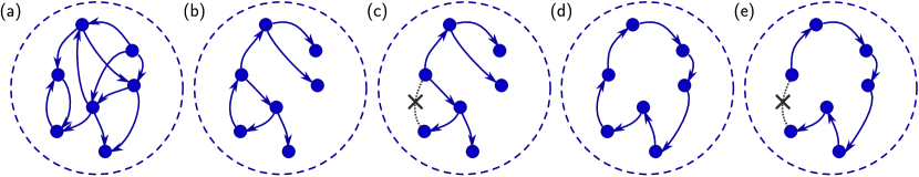
Figure 3: The five reservoir topologies tested. Only internal reservoir connections are pictured. Connections to the reservoir computer input, or to the output layer (as in Fig. 1) are not shown. (a) A general, fixed in-degree network, here pictured with $N=7$ and $k=2$. (b) A $k=1$ network with a single connected component. (c) A $k=1$ network with the single cycle cut at an arbitrary point. (d) A simple cycle reservoir. (e) A delay line reservoir.

Therefore, to create a random instantiation of a RC suitable to begin the training process, we must set a value for five hyperparameters:

• $\gamma$, which sets the characteristic time scale of the reservoir,

• $\sigma$, which determines the probability a node is connected to a reservoir input,

• $\rho_{\text{in}}$, which sets the scale of input weights,

• $k$, the recurrent in-degree of the reservoir network,

• $\rho_{r}$, the spectral radius of the reservoir network.

We select these parameters by searching a range of acceptable values selected to minimize the forecasting error using the Bayesian optimization procedure. The details of this can be found in Section IV.2. However, during the optimization process, we discovered that the optimizer was often finding RCs with $k=1$ that perform as well as RCs with a higher $k$. Such reservoirs have an interesting and simple network topology, thereby suggesting other simple topologies for comparison.

First, networks with $k=1$ generated with our algorithm often have disconnected components. These components essentially act as RCs operating in parallel; we do not consider these further even though it is an interesting line of research.Pathak et al. (2018) We limit ourselves to only looking at reservoir networks with a single connected component.

If a $k=1$ network only has a single connected component, then it must also contain only a single directed cycle. This limits how recurrence can occur inside the network compared to higher-$k$ networks. Every node in a $k=1$ network is either part of this cycle or part of a directed tree branching off from this cycle, as depicted in Fig. 3 (b). Inspired by the high performance of this simple structure, we also investigate $k=1$ networks when the single cycle is cut at an arbitrary point. This turns the entire network into a tree, as in Fig. 3 (c).

Finally, we also investigate reservoir networks that consist entirely of a cycle or ring with identical weights with no attached tree structure, depicted in Fig. 3 (d), and networks with a single line of nodes (a cycle that has been cut), in Fig. 3 (e). These are also known as simple cycle reservoirs and delay line reservoirs, respectively.Rodan and Tiňo (2011)

In total, there are five topologies we investigate:

1. general construction with unrestrained $k$,

2. $k=1$ with a single cycle,

3. $k=1$ with a cut cycle,

4. single cycle, or simple cycle reservoir,

5. single line, or delay line reservoir.

Both the $k=1$ cut cycle networks (c) and line networks (e) are rescaled to have a fixed $\rho_{r}$ before the cycle is cut. However, after the cycle is cut, they both have $\rho_{r}=0$.

IV.2 Bayesian Optimization

The choice of hyperparameters that best fits this problem is difficult to identify. Grid searchRodan and Tiňo (2011) and gradient descentJaeger et al. (2007) have been used previously. However, these algorithms struggle with either non-continuous parameters or noisy results. Because $W_{r}$ and $W_{\text{in}}$ are determined randomly, our optimization algorithm should be able to handle noise. We use Bayesian optimization,Yperman and Becker (2016); Maat, Gianniotis, and Protopapas (2018) as implemented by the skopt Python package.The scikit-optimize contributors (2018) Bayesian optimization deals well with both noise and integer parameters like $k$, is more efficient than grid search,Maat, Gianniotis, and Protopapas (2018) and works well with minimal tuning.

Table 1: Range of hyperparameters searched using Bayesian optimization.

Parameter	min		max
$\gamma$	7	–	11
$\sigma$	0.1	–	1.0
$\rho_{\text{in}}$	0.3	–	1.5
$k$	1	–	5
$\rho_{r}$	0.3	–	1.5

For each topology, the Bayesian algorithm repeatedly generates a set of hyperparameters to test within the ranges listed in Table 1. Larger ranges require a longer optimization time. We selected these ranges to include the values that existing heuristics would choose, and to allow exploration of the space without a prohibitively long runtime. However, exploring outside these ranges is valuable. Here we focus on the connectivity $k$, but expanding the search range for the other parameters may also produce interesting results.

At each iteration of the algorithm, the optimizer constructs a single random reservoir with the chosen hyperparameters, trains it according to the procedure described in Section IV.3, and measures its performance with the metric $\epsilon$ described in Section V. From this measurement, it chooses a new set of hyperparameters to test that may be closer to the optimal values. We limit the number of iterations of this algorithm to test a maximum of 100 reservoir realizations before returning an optimized reservoir. In order to estimate the variance in the performance of reservoirs optimized by this method, we repeat this process 20 times.

IV.3 Training

To train the RC, we integrate Eq. 1 coupled with the chosen input (Eqs. 6, 7 and 8) via the hybrid Runge-Kutta 5(4)Dormand and Prince (1980) method from $t=0$ to $300$ with a fixed time step $\Delta t=0.01$, and divide this interval into three ranges:

• $t=0$ – $100$: a transient, which is discarded,

• $t=100$ – $200$: the training period,

• $t=200$ – $300$: the testing period.

We use the transient period to ensure the later times are not dependent on the specific initial conditions. We divide the rest into a training period, used only during training, and a testing period, used later only to evaluate the RC performance.

This integration produces a solution for $\mathbf{r}(t)$. However, when the reservoir is combined with the Lorenz system, it has a symmetry that can confuse prediction.Pathak et al. (2017) Before integration, we break this symmetry by setting $\mathbf{f_{\text{out}}}$ so that

$$\tilde{r}_{i}(t)=\begin{cases}r_{i}(t)&\text{if }i\leq N/2,\\ r_{i}{(t)}^{2}&\text{if }i>N/2.\end{cases}$$ (10)

For consistency across our three example input systems, this is done for every reservoir we construct, even if the input system we eventually use is not the Lorenz system. We then find a $W_{\text{out}}$ to minimize

$$\sum_{t=100}^{200}|\mathbf{u}(t)-W_{\text{out}}\,\mathbf{\tilde{r}}(t)|^{2}+\alpha||W_{\text{out}}||^{2},$$ (11)

where the sum is understood to be over time steps $\Delta t$ apart. Now that $W_{\text{out}}$ is determined, the RC is trained.

Equation 11 is known as Tikhonov regularization, or ridge regression. The ridge parameter $\alpha$ could be included among the hyperparameters to optimize. However, unlike the other hyperparameters, modifying $\alpha$ does not require re-integration and can be optimized with simpler methods. We select an $\alpha$ from among $10^{-5}$ to $10^{5}$ by leave-one-out cross-validation. This also reduces the number of dimensions the Bayesian algorithm must work with.

V Forecasting and Evaluation

To evaluate the performance of the trained RC, we use it to perform autonomous forecasting using Eq. 5.

The most common method for evaluating an RC forecast is to choose a time $t_{1}$ to begin forecasting and then compare the forecast to the true system.Lukoševičius (2012) Usually, $t_{1}$ is chosen to be directly after the training period, which is $t_{1}=200$ in our procedure. Then, we initialize the reservoir state $\mathbf{r}(t_{1})$ to the value found earlier during training and integrate Eq. 5 for one Lyapunov time, between $t=t_{1}$ and $t=t_{1}+1/\lambda$. This produces a reservoir forecast $W_{\text{out}}\;\mathbf{\tilde{r}}(t)$ during these times, which we compare to the true system $\mathbf{u}(t)$ to produce a root-mean-squared error (RMSE)

$$\epsilon_{1}={\left(\Delta t\,\lambda\sum_{t=t_{1}}^{t_{1}+1/\lambda}|\mathbf{u}(t)-W_{\text{out}}\mathbf{\tilde{r}}(t)|^{2}\right)}^{1/2}.$$ (12)

Note that $\epsilon_{1}$ is normalized because we construct the input signal $\mathbf{u}(t)$ with unit variance.

This method of evaluating forecasting ability is flawed for our purposes. Previous results have shown that a low $\epsilon_{1}$ is not a good indicator of whether a reservoir computer has learned the climate of a systemPathak et al. (2017); Haluszczynski and Räth (2019) and we also observe the same effect here. Figure 4 depicts two common ways for an RC to fail to replicate the true Lorenz attractor, shown in Fig. 2. However, both produce a good short-term forecast near $t_{1}$. In particular, reservoir (ii) in Fig. 4 has a lower $\epsilon_{1}$ score than any of the optimized reservoirs despite its obvious failure to learn the Lorenz attractor.

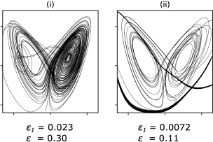
Figure 4: Two examples of reservoir computers that fail to reproduce the Lorenz climate, but produce a low $\epsilon_{1}$. Compare with the true attractor in Fig. 2. Reservoir (i) fails to learn the attractor, overemphasizing the right lobe in which $t_{1}$ resides. Reservoir (ii) matches the attractor well early on, but as the prediction lengthens, it falls into a periodic orbit (thick black line). Both (i) and (ii) show a promising low $\epsilon_{1}$, but the averaged $\epsilon$ measure more accurately captures their failure to learn the Lorenz attractor.

This problem is exacerbated in an optimization setting because searching for reservoirs with the lowest $\epsilon_{1}$ risks producing reservoirs that are only good at forecasts near $t_{1}$, but otherwise perform poorly in reproducing the climate. It can also waste time, as the optimization algorithm explores areas of the parameter space it believes perform well, but actually do not.

Finally, the choice of $t_{1}$ can dramatically affect $\epsilon_{1}$. For example, the Lorenz system has an unstable saddle point at the origin, and trajectories that approach this point may end up in either the left or right lobe of the attractor in Fig. 2. If $t_{1}$ happens to lie near this point, then even very small prediction errors can be magnified. For example, if the reservoir predicts a trajectory into the left lobe, while the true system goes to the right, the $\epsilon_{1}$ measure might be very high even though the reservoir is well-trained.

To combat these problems, we instead evaluate a short-term forecast at $50$ times $t_{i}$, evenly spaced within our testing period between $t=200\;\text{--}\;300$. For each $t_{i}$, we perform the evaluation method as described above, producing $50$ error measures $\epsilon_{i}$. Because each $t_{i}$ is drawn from the testing period, we only evaluate the reservoir on data it has not yet seen: no information about the input or reservoir system at $t_{i}$ is used to construct $W_{\text{out}}$.

We then combine these errors into a single overall error

$$\epsilon={\left(\frac{1}{50}\sum_{i=1}^{50}\epsilon_{i}^{2}\right)}^{1/2}$$ (13)

that represents the average ability of the reservoir computer to forecast accurately at any point on the input system attractor.

The parameter $\epsilon$ is our figure of merit that the Bayesian algorithm is trying to minimize. By combining short-term forecasting errors from many points on the input attractor, this metric emphasizes learning the global dynamics of the system as opposed to short-term forecasting over a single temporal segment. Using this method, we see that the Bayesian optimization algorithm works more effectively, as it no longer gets trapped in valleys of low $\epsilon_{1}$ that otherwise fail to reproduce the attractor. This evaluation method is summarized in Fig. 5.

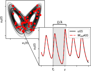
Figure 5: Summary of our forecasting evaluation method. We calculate errors $\epsilon_{i}$ at times $t_{i}$, marked on the attractor as red dots, and combine them into a single error $\epsilon$. Before each $t_{i}$ (dotted vertical line), the reservoir is integrated with Eq. 1 and listening to the input. After $t_{i}$, the reservoir is integrated with Eq. 5, and runs autonomously. The reservoir’s prediction (dotted red line) must eventually diverge from the true system (solid black line). We calculate $\epsilon_{i}$ only during a single Lyapunov period after forecasting begins, marked here in grey.

VI Results

We run all five reservoir topologies through 100 iterations of the Bayesian algorithm using the Lorenz system as input, and record the best-performance RC for each topology according to the metric $\epsilon$. These reservoirs, and the hyperparameters that generated them, are reported in Table 2. We estimate the errors on these with the standard deviation of $\epsilon$ after repeating the optimization process 20 times.

Table 2: Best reservoir computers of each topology, after 100 iterations of the Bayesian optimization algorithm using the Lorenz system as input. The hyperparameters chosen by the algorithm are shown on the right. The simpler topologies (b) – (e) all perform nearly as well as the general topology (a).

		Lorenz
	Topology	$\epsilon$	$\gamma$	$\sigma$	$\rho_{\text{in}}$	$\rho_{r}$
(a)	Any $k$	0.022 $\pm$ 0.004	$7.7$	$0.81$	$0.37$	$0.41$
(b)	$k=1$ with cycle	0.024 $\pm$ 0.005	$10.9$	$0.44$	$0.30$	$0.30$
(c)	$k=1$ no cycle	0.028 $\pm$ 0.005	$7.2$	$0.78$	$0.30$	$0.30$
(d)	cycle	0.023 $\pm$ 0.008	$7.9$	$0.17$	$0.58$	$0.30$
(e)	line	0.024 $\pm$ 0.003	$10.6$	$0.79$	$0.30$	$0.45$

When optimized, all reservoir topologies perform well. In particular, the simpler topologies all perform almost as well as the general-$k$ topology. They often lie within one, or at most two standard deviations from topology (a). This is despite the fact that topologies (c) and (e) both have $\rho_{r}=0$ and no recurrent connections within the network. The other topologies have $\rho_{r}\ll 1$. Previous work has already demonstrated that reservoirs with low or zero spectral radius can still function.Pathak et al. (2017); Rodan and Tiňo (2011) These results act as additional counterexamples to the heuristic that reservoir computers should have $\rho_{r}\approx 1$.Lukoševičius (2012)

However, these best-observed reservoirs are not representative of a typical RC. We use the hyperparameters to guide the random input connections and connections within the reservoir, and so even once the hyperparameters are fixed, constructing the reservoir is a random process. Not all reservoirs with a fixed topology and hyperparameters will perform the same.

To explore this variation, we generate and evaluate $200$ RCs of each topology on the Lorenz system, using the optimized hyperparameters in Table 2. For all five topologies, as the measured $\epsilon$ increases, the quality of the reproduced attractor decreases gradually. On manual inspection of the attractors, the reason for this decrease can be divided into three qualitative regions. For $\epsilon<0.3$, the RCs reproduce the Lorenz attractor consistently. Failures still rarely occur, but they always reproduce part of the attractor before falling into a fixed point or periodic orbit. In this region, small differences between the true attractor and the reproduced attractor contribute more to $\epsilon$ than outright failure. For $0.3<\epsilon<1.0$, RCs always fail to reproduce the attractor, though they will still always reproduce a portion of it before failing. Examples of these failures are provided in Fig. 4. Above $\epsilon>1.0$, these failures become catastrophic, and no longer resemble the Lorenz attractor at all. A more quantitative description of these regions is one line of possible future research.

Though the optimized best-performing reservoirs of each topology show very little performance difference, the differences between them become more apparent when we compare the probability distribution of $\epsilon$ for each topology. These distributions are shown in Fig. 6.

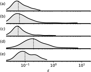
Figure 6: Performance for each reservoir topology, evaluated for the Lorenz system at the hyperparameters listed in Table 2. Each is visualized as a Gaussian kernel density estimation in $\log_{10}\epsilon$ with a bandwidth of 0.35,Scott (1992) which can be interpreted as a probability distribution. Using a narrower bandwidth does not reveal additional features. A vertical line marks the median. Note that topologies (b) – (e) have very long tails, and can produce reservoirs that perform very poorly in comparison to (a). However, all five have the capability to produce well-performing reservoirs.

A well-performing reservoir with arbitrary $k$ (a) is a much more likely outcome than a well-performing reservoir with a single cycle (d). However, the performance of arbitrary $k$ reservoirs (a) is very similar to that of tree-like reservoirs (c). Though (c) has a longer tail on the high end, the simpler structure of the reservoir may be appealing for hardware RCs.

The distribution of performance for each topology can be a deciding factor if reservoir construction and evaluation is expensive, as it might be in hardware. In software, though, we find the best-performing reservoirs in Table 2 after only $100$ trials. A hardware design can still benefit from the simpler topologies (b) – (e) despite their very wide performance distributions if the creation of the evaluation of the design can be automated to test many candidate reservoirs, as on an FPGA.Canaday, Griffith, and Gauthier (2018)

Figure 7: Lorenz attractor plots in the $x$/$z$ plane for long-term free-running predictions for each reservoir topology in Table 2. Compare with true Lorenz attractor in Fig. 2, and the failed reservoirs in Fig. 4.

There may also be a benefit in software. The simpler topologies are represented by weight matrices $W_{r}$ in very simple forms. Topology (c) can always be represented as a strictly lower-diagonal matrix, and (d) – (e) can be represented with non-zero entries only directly below the main diagonal. Software simulations can take advantage of this structure to speed up integration of Eq. 1.

To explore whether these topologies remain equally effective at tasks beyond forecasting the Lorenz system, we run all five reservoir topologies through 100 iterations of the Bayesian algorithm for both the Rössler and the double-scroll systems. As with the Lorenz system, we estimate the errors on these results by repeating the process 20 times each. These results are reported in Table 3.

Table 3: Result of optimizing reservoirs with the Bayesian algorithm over 100 iterations, on both the Rössler system and the double-scroll system. All five topologies can perform equally well at both systems.

		Double Scroll	Rössler
	Topology	$\epsilon$	$\epsilon$
(a)	Any $k$	0.029 $\pm$ 0.006	0.017 $\pm$ 0.005
(b)	$k=1$ with cycle	0.033 $\pm$ 0.007	0.020 $\pm$ 0.007
(c)	$k=1$ no cycle	0.033 $\pm$ 0.008	0.018 $\pm$ 0.006
(d)	cycle	0.033 $\pm$ 0.007	0.018 $\pm$ 0.006
(e)	line	0.037 $\pm$ 0.01	0.019 $\pm$ 0.015

The results for the double-scroll and Rössler systems agree well with those for Lorenz. All five topologies optimize reliably with the Bayesian algorithm, and all perform similarly when optimized. Optimizing a reservoir to reproduce either system will almost always work after only 100 iterations.

One advantage to RCs is that a single reservoir can be re-used on many different tasks by re-training $W_{\text{out}}$. To evaluate whether this is possible with these optimized reservoirs, we take the 20 reservoirs optimized for the Lorenz system and re-train $W_{\text{out}}$ for each to instead reproduce the double-scroll circuit system. Every other part of the RC is left unchanged. We then evaluate how accurate this prediction is using the metric $\epsilon$. These results are summarized in Table 4.

Table 4: Result of re-using reservoirs optimized for Lorenz prediction to perform double-scroll prediction. The minimum error encountered across all 20 reservoirs of each topology is reported as $\epsilon_{\text{min}}$.

		Double Scroll
	Topology	$\epsilon$	$\epsilon_{\text{min}}$
(a)	Any $k$	0.43 $\pm$ 1.2	0.028
(b)	$k=1$ with cycle	0.30 $\pm$ 0.5	0.048
(c)	$k=1$ no cycle	0.37 $\pm$ 0.8	0.032
(d)	cycle	0.17 $\pm$ 0.2	0.056
(e)	line	0.22 $\pm$ 0.3	0.058

In general, these reservoirs perform poorly on this new task. However, there is extremely high variation. Even though they were optimized to perform Lorenz forecasting, many of these reservoirs are still able to reproduce the double-scroll attractor. Moreover, the best performers in each category approach the performance of reservoirs optimized specifically for the double-scroll system. This indicates that it is possible to find a single reservoir in any of these topologies that works well on more than one system. The Bayesian optimization algorithm may be able to find these reservoirs more reliably if the metric $\epsilon$ is modified to reward RCs that perform well on many systems.

Finally, for each topology produced a free-running prediction of the Lorenz system for $100$ time units using the best-performing RC. We use these predictions to produce an attractor as shown in Fig. 7. All five optimized RCs reproduce the Lorenz attractor well. Though comparing these plots by eye is not quantitative, we find them qualitatively useful: an RC that fails to reproduce the Lorenz attractor by eye is unlikely to have a low $\epsilon$ compared to one that does.

VII Conclusion

We find that Bayesian optimization of RC hyperparameters is a useful tool for creating high-performance reservoirs quickly. We also find that allowing the optimizer to explore areas of the parameter space that are typically excluded in other optimization studies can lead to interesting and effective reservoir designs such as those presented here.

For this procedure to be effective, we find that evaluating the RC performance at many points along the attractor and averaging, rather than at a single point, encourages the optimization algorithm to find reservoirs that reproduce the Lorenz climate. Using this evaluation method helps direct the optimizer away from reservoirs that perform good short-term forecasting at only one point on the Lorenz attractor.

One surprising outcome of our optimization procedure is finding reservoirs that perform well even with no recurrent connections and $\rho_{r}=0$. Though some reservoirs of this kind have been explored previously and shown to work,Pathak et al. (2017); Rodan and Tiňo (2011) the heuristics remain common in reservoir design. We present additional concrete examples that provide evidence these heuristics are not unbreakable rules.

In greater detail, we find reservoirs with very low internal connectivity that perform at least as well as their higher-connectivity counterparts. A reservoir with only a single internal cycle, or even no cycle at all, can perform as well as those with many recurrent cycles. These simpler topologies manifest as simpler weight matrices, which can result in faster integration in software. In a hardware environment where connections between nodes have a cost, or recurrence is difficult to implement, these network topologies may also have a direct benefit.

Though the best of these low-connectivity reservoirs perform as well as the more complicated reservoirs, they tend to perform worse on average. However, searching for the best-performing instance of these reservoirs can be done in few trials, and may be feasible for hardware reservoirs that can be constructed and evaluated in an automated way.

We have discovered many interesting lines of future research. First, we can evaluate the new metric $\epsilon$ by comparing the output of the reservoir predictions to the true system attractor using a new metric for attractor overlap.Ishar et al. (2019) This overlap metric can also be used to quantify the qualitative observations of different failure modes in regions of our $\epsilon$ metric. Second, there are known results that prove that a linear network architecture with time-independent nodes, the discrete-time NARX networks, can simulate fully-connected networks.Siegelmann, Horne, and Giles (1997) There may be a similar proof for RCs, which might explain why we see no difference in the best-performing reservoirs in each topology. Third, our optimization procedure finds the best network weights $W_{r}$ for a given task. In many ways, this is a similar task to training a traditional recurrent neural network. We are interested in comparing this method to those used for networks other than RCs.

Our results show that these very low connectivity reservoirs perform well in the narrow context of software-based, chaotic system forecasting. Future work will explore whether these results hold for other reservoir computing tasks such as classification, and whether it is possible to find reservoirs that perform well on a variety of tasks simultaneously by modifying the metric $\epsilon$ to encourage generalization. We also intend to explore whether these results hold in hardware reservoirs and if the simpler reservoir designs allow for more efficient and faster operating hardware RCs.