Confidence intervals for median absolute deviations

Abstract

The median absolute deviation (MAD) is a robust measure of scale that is simple to implement and easy to interpret. Motivated by this, we introduce interval estimators of the MAD to make reliable inferences for dispersion for a single population and ratios and differences of MADs for comparing two populations. Our simulation results show that the coverage probabilities of the intervals are very close to the nominal coverage for a variety of distributions. We have used partial influence functions to investigate the robustness properties of the difference and ratios of independent MADs.

Keywords: asymptotic variance, partial influence functions, robust

1 Introduction

The median absolute deviation is a robust measure of dispersion (MAD, see e.g. Hampel,, 1974; Hampel et al. ,, 1986). Defined as the median of the absolute residuals from the median, the MAD is a suitable scale measure to accompany the median. Hampel, (1974) referred to the MAD as the “median deviation” and it had first received attention even as early as Gauss, (1816), and later rediscovered by Hampel, (1968). The MAD is the most robust estimator of scale as measured by robustness measures such as the break-down point and gross error sensitivity (Hampel,, 1974). The breakdown point of an estimator is the proportion of contamination that the estimator can handle before providing unreliable results and for the MAD this is equal to 1/2 (the maximum). The MAD estimator has what is known as a bounded influence function so that the amount of influence any observational type can exert on the estimator is limited. More will be said on the influence function later.

Arachchige et al. , (2019a) showed that excellent coverages for interval estimators of ratios of interquantile ranges can be achieved. This makes these intervals more suitable than those for ratio of variances when normality cannot be assumed. Then, Arachchige et al. , (2019b) considered interval estimators for robust versions of the coefficient of variation, one of which uses the MAD in place of the standard deviation (and the median to replace the mean). Motivated by these good coverage properties, we consider interval estimators for the MAD and for ratios and differences of independent MADs as robust alternatives to intervals based on sample variances. To the best of our knowledge, and not to confuse the MAD with the mean absolute deviation for which interval estimators with good coverage have been introduced by Bonett & Seier, (2003), no one has introduced these interval estimators for the MAD. The very good coverage properties, that we will highlight later, ensure inferences about dispersion based on the MAD are possible.

In Section 2 we provide some necessary notations before considering influence functions for ratios of MADs. In Section 3 we consider confidence intervals for MADs, differences of MADs and ratios of MADs with coverage properties explored via simulations in Section 4. Examples are also considered in Section 4 and we conclude in Section 5.

2 Notations and influence functions

Let $X$ denote a random variable and $F$ its distribution function. Then Hampel, (1974) defined the median absolute deviation (MAD) as

$$\hbox{MAD}(X)=\text{med}\mid{X-M}\mid~{},$$ (2.1)

where ‘med’ denotes the median and $M=\text{med}(X)=F^{-1}(0.5)$ is the population median. Let $X_{1},\ldots,X_{n}$ denote a random sample of $n$ observations. Then the MAD estimate is simply the median of the absolute residuals from the sample median. That is, for $m$ denoting the sample median, $\widehat{\text{MAD}}$ is the sample median of the $|X_{1}-m|,\ldots,|X_{n}-m|$. While inference, for a single MAD may be of interest, it is often that case that comparison of dispersion measures, such as the MAD, is needed to compare two populations.

Consider two independent random variables $X\sim F_{1}$ and $Y\sim F_{2}$ and let us consider $\hbox{MAD}(X)$ and $\hbox{MAD}(Y)$. Then, the population squared ratio of MADs, which we denote as $R_{M}$, and associated estimator can be define as

$$R_{M}=\left[\frac{\hbox{MAD}(X)}{\hbox{MAD}(Y)}\right]^{2}\;\;\text{and}\;\;\widehat{R}_{M}=\left[\frac{\widehat{\hbox{MAD}(X)}}{\widehat{\hbox{MAD}(Y)}}\right]^{2}.$$ (2.2)

Here we have suggested the squared ratio of MADs since it is the analogue to the ratio of variances and, in fact, equal to ratio of variances for some distributions (e.g. normal). However, the ratio of MADs may also be used. Another possibility is the difference of MADs, $D_{M}$, where

$$D_{M}=\hbox{MAD}(X)-\hbox{MAD}(Y)\;\;\text{and}\;\;\widehat{D}_{M}=\widehat{\hbox{MAD}(X)}-\widehat{\hbox{MAD}(Y)}~{}.$$ (2.3)

2.1 Influence function and partial influence functions

Define the contamination distribution to be $F_{\epsilon}=(1-\epsilon)F+\epsilon\Delta_{x}$, where $\epsilon\in[0,1]$ is the proportion of contamination and $\Delta_{x}$ has all of its mass at the contaminant $x$. Consider an estimator functional $\mathcal{T}$ such that $\mathcal{T}(F)=\theta$ and $\mathcal{T}(F_{n})=\widehat{\theta}$ where $F_{n}$ denotes the empirical distribution function for sample of $n$ observations. The relative influence on $\mathcal{T}(F)$ of $\epsilon$ proportion of contaminated observations at $x$ is given by, $[\mathcal{T}(F_{\epsilon})-\mathcal{T}(F)]/\epsilon$, where $\mathcal{T}(F_{\epsilon})=(1-\epsilon)\mathcal{T}(F)+\epsilon\Delta_{x}$. Then, the influence function (IF Hampel,, 1974) is defined as,

$$\hbox{IF}(x;\mathcal{T},F)=\lim_{\epsilon\downarrow 0}\frac{\mathcal{T}(F_{\epsilon})-\mathcal{T}(F)}{\epsilon}\equiv\frac{\partial}{\partial\epsilon}\mathcal{T}(F_{\epsilon})\Big{|}_{\epsilon=0}.$$

When more than one population exists, the IF is determined by contaminating one population while the other population remains uncontaminated. Pires & Branco, (2002) defines this notion as “partial IFs” (PIFs) and in our context with two populations we have two PIFs. The first PIF of the estimator with functional $\mathcal{T}$ at ($F_{1},\ F_{2}$) is

$$\text{PIF}_{1}(x;\mathcal{T},F_{1},F_{2})=\lim_{\epsilon\to 0}\left[\frac{\mathcal{T}[(1-\epsilon)F_{1}+\epsilon\Delta_{x_{0}},F_{2}]-\mathcal{T}(F_{1},F_{2})}{\epsilon}\right]$$ (2.4)

and with $\text{PIF}_{2}(x;\mathcal{T},F_{1},F_{2})$ defined similarly.

Now, consider the functional for the standardized MAD denoted by $\mathcal{MAD}$ so that $\mathcal{MAD}(F)=\hbox{MAD}_{X}$. Hampel, (1974) gives the influence function for the MAD when $F$ is the normal distribution and further details can be found on page 107 of Hampel et al. , (1986). Let $f=F^{\prime}$ denote the density function then, assuming $f(M)$ and $2[f(M+\text{MAD}_{X})+f(M-\text{MAD}_{X})]$ are nonzero, a general form of the IF for the MAD exists; e.g. see page 137 of Huber, (1981) or page 16 of Andersen, (2008). This is given as

$$\hbox{IF}(x;\,\mathcal{MAD},F)=\displaystyle\frac{\left[\text{sign}(x-M)-\text{MAD}_{X}\right]-\displaystyle\frac{f(M+\text{MAD}_{X})-f(M-\text{MAD}_{X})}{f(M)}\text{sign}(x-M)}{2[f(M+\text{MAD}_{X})+f(M-\text{MAD}_{X})]}.$$ (2.5)

2.1.1 Partial influence functions of the difference and squared ratio of MADs

Let $\mathcal{D}_{M}$ be the functional for the difference of MADs so that,

$$\mathcal{D}_{M}(F_{1},F_{2})=\mathcal{MAD}(F_{1})-\mathcal{MAD}(F_{2})~{}$$

then the PIFs are $\text{PIF}_{1}(x;\mathcal{D}_{M},F_{1},F_{2})=\hbox{IF}(x;\mathcal{MAD},F_{1})$ and $\text{PIF}_{2}(x;\mathcal{D}_{M},F_{1},F_{2})=-\hbox{IF}(x;\mathcal{MAD},F_{2})$. These are trivial and previous studies on robustness of the MAD may be considered for this context. We therefore do not explore the difference PIFs further.

Let $\mathcal{R}_{M}$ be the functional for the squared ratio of MADs so that,

$$\mathcal{R}_{M}(F_{1},F_{2})=\left[\frac{\mathcal{MAD}(F_{1})}{\mathcal{MAD}(F_{2})}\right]^{2}~{}.$$

Then the PIFs for the squared ratio of MADs are given below.

Theorem 2.1.

For $\text{PIF}(x;T,F_{1},F_{2})$ as defined in (2.4), the PIFs of $\mathcal{R}_{M}$ are

$$\text{PIF}_{1}(x;\mathcal{R}_{M},F_{1},F_{2}) =\frac{2\,\mathcal{R}_{M}(F_{1},F_{2})}{\mathcal{MAD}(F_{1})}\hbox{IF}(x;\mathcal{MAD},F_{1}),$$

$$\text{PIF}_{2}(x;\mathcal{R}_{M},F_{1},F_{2}) =-\frac{2\,\mathcal{R}_{M}(F_{1},F_{2})}{\mathcal{MAD}(F_{2})}\hbox{IF}(x;\mathcal{MAD},F_{2}).$$

The proof of Theorem 2.1 is in Appendix A.2 and we consider some examples of the first PIF next.

2.1.2 Partial influence functions comparison

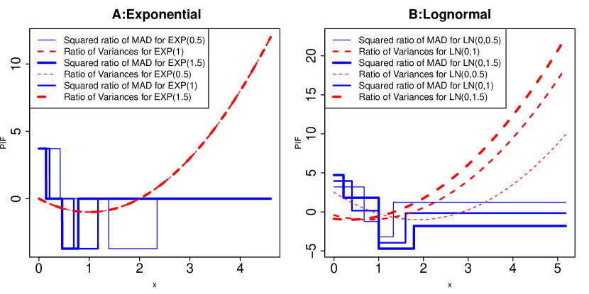
Figure 1: PIF₁ comparisons for (A) two exponential populations both with rates 0.5, 1 and 1.5 and (B) two log-normal populations both with $\mu$=0 and $\sigma$=0.5,1,1.5.

Figure 1 depicts the PIFs of the first population for the squared ratio of MADs and the ratio of variances (see Arachchige et al. ,, 2019a, for these). In Plot A we consider the ratio of variances and squared ratio of MADs for two exponential distributions, both with rates equal to 0.5, or 1 or 1.5. Similarly, in Plot B we do this for two log normal distributions both with $\mu$=0 and $\sigma=0.5$ or 1 or 1.5. Since the numerator and denominator distributions are the same, both are estimators of one and therefore the PIFs are comparable. As expected, the PIFs of the ratio of variances is unbounded indicating that outliers can exert large influence on the estimator. The PIFs of the squared ratio of MAD is bounded and the influence of any large outliers is limited, and far less than for the ratio of variances. For the exponential distribution, the PIFs of ratio of variances do not depend on the rate parameter. However, for the log-normal distribution the PIF for the ratio of variances increases quickly with increasing $\sigma$.

3 Asymptotic confidence intervals

In their discussion of intervals for the mean absolute deviations, Bonett & Seier, (2003) provide suggestions for median absolution deviations from a fixed point, $h$. They suggest using intervals for the median and where the data used is the transformed $|X_{i}-h|$s. When $h$ is the population median, i.e. $h=M$, and this median is known, simulations (not shown) result in good coverage that is close to nominal. However, when $M$ is not known and needs to be estimated, this approach typically results in coverage that is too low (e.g. less than 0.8 for a nominal 0.95). In this section we therefore provide confidence intervals that have good coverage properties, as shown by our simulations that follow.

Asymptotic normality and associated variance of the MAD can be found in Falk, (1997) who provide the asymptotic joint normality between the median and MAD estimators. We again let $\text{MAD}_{X}=\mathcal{MAD}(F)$ and also let $\mathcal{MAD}(F_{n})=\widehat{\text{MAD}}_{X}$. Then, if $F$ is continuous near, and differentiable at, the median $M$, $M-\hbox{MAD}_{X}$ and $M+\hbox{MAD}_{X}$ with $f(M)>0$ and $B_{1}=f(M-\hbox{MAD}_{X})+f(M+\hbox{MAD}_{X})>0,$ we have

$$\sqrt{n}\left(\widehat{\text{MAD}}_{X}-\hbox{MAD}_{X}\right)\stackrel{{\scriptstyle\text{\tiny approx.}}}{{\sim}}N(0,\hbox{ASV})~{},$$

where ‘$\stackrel{{\scriptstyle\text{\tiny approx.}}}{{\sim}}$’ denotes ‘approximately distributed’. The asymptotic variance of the MAD estimator is

$$\hbox{ASV}=\hbox{ASV}(\mathcal{MAD};F)=\frac{1}{4B_{1}^{2}}\left[1+\frac{B_{2}}{\left[f(M)\right]^{2}}\right]~{},$$ (3.1)

where $B_{1}$ is given above and $B_{2}=B_{3}^{2}+4B_{3}f(M)\left[1-F(M+\hbox{MAD}_{X})-F(M-\hbox{MAD}_{X})\right]$ with $B_{3}=f(M-\hbox{MAD}_{X})-f(M+\hbox{MAD}_{X})$.

We used the ASV in (3.1) and the Delta method (see e.g., chapter 3 of DasGupta,, 2006) to derive the asymptotic variance of the ratios of MADs. The asymptotic variance of $\sqrt{n_{1}+n_{2}}\mathcal{R}_{M}(F_{n_{1}},F_{n_{2}})$ is

$$\hbox{ASV}(\mathcal{R}_{M};n_{1},n_{2})=4\mathcal{R}^{2}_{M}(F_{1},F_{2})\Bigg{[}\frac{\hbox{ASV}(\mathcal{MAD},F_{1})}{w_{1}\,\mathcal{MAD}^{2}(F_{1})}+\frac{\hbox{ASV}(\mathcal{MAD},F_{2})}{w_{2}\,\mathcal{MAD}^{2}(F_{2})}\Bigg{]}~{}$$ (3.2)

where $w_{i}=n_{i}/(n_{1}+n_{2})$ for $i=1,2$.

Since the two populations are independent, deriving the asymptotic variance of the difference of MAD is straightforward.

$$\hbox{ASV}(\mathcal{D}_{M};n_{1},n_{2})=\hbox{ASV}(\mathcal{MAD},F_{1})+\hbox{ASV}(\mathcal{MAD},F_{2}).$$ (3.3)

Throughout, let $\widehat{\text{ASD}}(\cdot)=\sqrt{\widehat{\text{ASV}}(\cdot)}$ denote the estimated asymptotic standard deviation estimate. Note that the ASV depends on both $f$ and $F$, the density and distribution functions. There are several options to estimate these, but we choose to use the very flexible Generalized Lambda Distribution (GLD) which, for the FKML parameterization (Freimer et al. ,, 1988), is defined in terms of its quantile function, $Q(p)$,

$$Q(p)=\lambda_{1}+\lambda_{2}^{-1}\left\{\lambda_{3}^{-1}(p^{\lambda_{3}}-1)-\lambda_{4}^{-1}[(1-p)^{\lambda_{4}}-1]\right\}~{},$$

where $\lambda_{1}$, $\lambda_{2}$, $\lambda_{3}$ and $\lambda_{4}$ are the location, inverse scale and two shape parameters respectively. To estimate the GLD parameters we use a recent approach introduced by Dedduwakumara et al. , (2019a) which is computationally efficient making it useful for our simulations that follow. However, other estimators can also be used. We then use these parameter estimates with the density and distribution functions for the GLD in R gld package (King et al. ,, 2016).

Based on asymptotic normality of the MAD (e.g. Falk,, 1997), an asymptotic $(1-\alpha)\%$ confidence interval for MAD is given as

$$[L,U]_{\hbox{MAD}}=\Bigg{[}\widehat{\hbox{MAD}}_{X}\pm z_{1-\alpha/2}\;\frac{\widehat{\hbox{ASD}}{(\mathcal{MAD},F_{n})}}{\sqrt{n}\,}\Bigg{]}~{},$$ (3.4)

where the $z_{1-\alpha/2}$ is the $(1-\alpha/2)\times$100 percentile of the standard normal distribution.

When constructing the interval estimator for the squared ratio of MADs, we first derive the confidence interval for the log transformed ratio and then exponentiate to return to the ratio scale. Let $\mathcal{W}(F_{1},F_{2})=\ln[\mathcal{R}_{M}(F_{1},F_{2})]$ then, using the Delta method, it is straightforward to show that $\hbox{ASV}(\mathcal{W},F_{1},F_{2})\doteq\hbox{ASV}(\mathcal{R}_{M},F_{1},F_{2})/[\mathcal{R}_{M}(F_{1},F_{2})]^{2}$ . Then a $(1-\alpha)\%$ confidence interval estimator for $R_{M}$ is given as

$$[L,U]_{R_{M}}=\exp\Bigg{[}\ln(\widehat{R}_{M})\pm z_{1-\alpha/2}\;\frac{\widehat{\hbox{ASD}}{(\mathcal{R}_{M},F_{n_{1}},F_{n_{2}})}}{\widehat{R}_{M}\sqrt{n_{1}+n_{2}}\,}\Bigg{]}~{},$$ (3.5)

where $\widehat{R}_{M}$ is the squared ratio of MADs estimator and the ASV is in (3.2).

Finally, a $(1-\alpha)\%$ confidence interval for the difference in MADs is simply

$$[L,U]_{D_{M}}=\widehat{D}_{M}\pm z_{1-\alpha/2}\;\frac{\widehat{\hbox{ASD}}{(\mathcal{D}_{M},F_{n_{1}},F_{n_{2}})}}{\sqrt{n_{1}+n_{2}}\,}~{},$$ (3.6)

where $\widehat{D}_{M}$ is the difference of MADs estimator and the ASV can be found in (3.3).

4 Simulations and Examples

We begin by conducting simulations to assess the coverage properties of the interval estimations for data generated from several distributions. As pointed out earlier, we have used a new estimator of the GLD parameters provided by Dedduwakumara et al. , (2019b) since it exhibits very good performance and is very efficient making it useful for our simulations. In Appendix A.2, we provide R code for the interval estimators using readily available estimators for the GLD from the gld package (King et al. ,, 2016). In that code we have opted for Titterington’s method (Titterington,, 1985) since it to has good performance, albeit is more time consuming.

4.1 Simulations

To investigate the performance of the MAD, squared ratio of MADs and difference of MADs intervals we consider simulated coverage probability and the average confidence interval width as performance measures. We have selected the log normal (LN), exponential (EXP), chi-square ($\chi^{2}_{5}$) and Pareto (PAR) distributions with different sample sizes of $n=50,100,200,500,1000$. Each simulation consists of 10,000 trials.

Table 1: Simulated coverage probabilities (and widths in parentheses) for the 95% confidence interval for the MAD (* denotes median width reported due to excessively large widths for a small number of intervals that skew the mean).

Sample size	$X\sim$ LN(0,1)	$X\sim$ EXP(1)	$X\sim\chi^{2}_{5}$	$X\sim$ PAR(1,7)
True $\hbox{MAD}=$	0.599	0.481	1.895	0.075
50	0.938 (1.43)	0.936 (1.93)	0.927 (1.25*)	0.939 (0.34)
100	0.940 (0.37)	0.939 (0.29)	0.938 (0.91)	0.939 (0.05)
200	0.938 (0.26)	0.947 (0.20)	0.942 (0.65)	0.944 (0.03)
500	0.945 (0.16)	0.948 (0.12)	0.947 (0.41)	0.949 (0.02)
1000	0.946 (0.12)	0.951 (0.09)	0.944 (0.29)	0.947 (0.01)

Simulated coverages and widths for the interval estimator of MADs, from (3.4), are provided in Table 1 for several distributions. The coverage probabilities are all close to the nominal level of 0.95, even for $n=50$ where coverages were approximately in the vicinity of 0.93-0.94. Coverages become closer to the nominal level as the sample size increases and, as expected the interval widths decrease with increasing sample size.

Table 2: Simulated coverage probabilities (and widths in parentheses) for the 95% confidence interval for the squared ratio of MADs ($R_{M}$) and difference of MADs ($D_{M}$) (* Median width reported due to excessively large widths for a small number, between 1% and 2%, of intervals).

Sample sizes		$X\sim$ LN(0,1)	$X\sim$ EXP(1)	$X\sim\chi^{2}_{5}$	$X\sim$ PAR(1,7)
($n_{1}$,$n_{2}$)	Measure	$Y\sim$ LN(0,1)	$Y\sim$ EXP(1)	$Y\sim\chi^{2}_{2}$	$Y\sim$ PAR(1,3)
	True $R_{M}=$	1	1	3.876	0.148
	True $D_{M}=$	0	0	0.932	-0.119
50,50	$R_{M}$	0.958 (3.71*)	0.971 (4.03*)	0.955 (12.14*)	0.978 (0.91*)
	$D_{M}$	0.967 (2.55)	0.972 (3.49)	0.956 (1.54*)	0.967 (1.17)
100,100	$R_{M}$	0.949 (2.23)	0.958 (1.87*)	0.954 (6.48*)	0.960 (0.33*)
	$D_{M}$	0.954 (0.52)	0.958 (0.42)	0.952 (1.08)	0.951 (0.16)
200,200	$R_{M}$	0.953 (1.37)	0.946 (1.28)	0.950 (4.51)	0.952 (0.22)
	$D_{M}$	0.945 (0.37)	0.950 (0.28)	0.950 (0.76)	0.947 (0.10)
200,500	$R_{M}$	0.946 (1.09)	0.951 (1.02)	0.950 (3.47)	0.952 (0.17)
	$D_{M}$	0.945 (0.31)	0.951 (0.23)	0.946 (0.69)	0.956 (0.07)
500,500	$R_{M}$	0.946 (0.81)	0.952 (0.75)	0.949 (2.69)	0.950 (0.12)
	$D_{M}$	0.948 (0.23)	0.953 (0.17)	0.950 (0.48)	0.947 (0.06)
500,1000	$R_{M}$	0.947 (0.69)	0.952 (0.64)	0.948 (2.23)	0.951 (0.10)
	$D_{M}$	0.947 (0.20)	0.949 (0.15)	0.949 (0.45)	0.948 (0.04)
1000,1000	$R_{M}$	0.947 (0.56)	0.949 (0.52)	0.949 (1.87)	0.950 (0.09)
	$D_{M}$	0.944 (0.16)	0.950 (0.12)	0.952 (0.34)	0.948 (0.04)

Simulated coverages for interval estimators of squared ratio of MADs and difference of MADs are provided in Table 2 for several distributions. Results show excellent coverages compared to the coverages of F-test (the coverage probabilities for interval estimator of the $F$-test can be found in Table 3 of Arachchige et al. ,, 2019a) which are poor due to the violation of underlying normality assumptions). Coverages are very close to the nominal 0.95 for both the squared MAD ratio and difference of MAD for all the selected distributions, including smaller sample sizes. There are some slightly conservative coverages only for $n=50$ and for other sample sizes the coverages become very close. For smaller sample sizes a very small number of the intervals were very wide (between 1% and 2%) so we report the median width instead.

4.2 Prostate data example

The prostate data set, which is available in the depthTools package (Lopez-Pintado & Torrente,, 2013), is a normalized subset of the Singh et al. , (2002) prostate data set. The data consists of gene expressions for the 100 most variable genes for 25 normal and 25 tumoral samples.

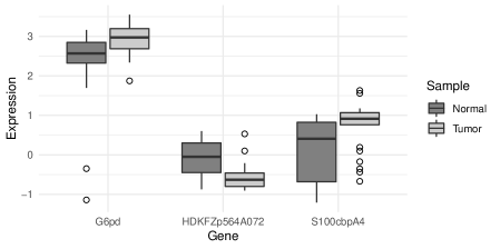
Figure 2: Box plots of three interesting genes selected from the prostate data set.

We selected three genes that are interesting when comparing intervals for ratios of variances and those based on the MADs. These three genes are three of the six that were considered by Arachchige et al. , (2019a). The genes and their abbreviations we consider are Glucose-6-phosphate dehydrogenase (G6pd), HDKFZp564A072 and calcium-binding protein A4 (S100cbpA4). Box plots of the genes are provided in Figure 2 where we note that, ignoring extreme outliers, the spread for the bulk of the data looks similar for G6pd and very different for HDKFZp564A072 and S100cbpA4.

Table 3: 95% asymptotic confidence intervals (CI) for the ratios of variances resulting from the $F$-test ($F$), the ratio of MADs ($R_{M}$) and difference of MADs ($D_{M}$) for the three selected genes.

	$F$		$R_{M}$		$D_{M}$
Gene	Est.	CI	Est.	CI	Est.	CI
G6pd	6.496	(2.863, 14.742)	1.000	(0.268, 3.734)	0.000	(-0.185, 0.185)
HDKFZp564A072	1.930	(0.850, 4.379)	5.013	(1.211, 20.761)	0.213	( 0.035, 0.391)
S100cbpA4	1.748	(0.770, 3.968)	8.725	(1.440, 52.856)	0.301	( -0.013, 0.615)

In Table 3 we provide the point estimate and asymptotic 95% confidence intervals for the ratio of variances (from the $F$-test assuming underlying normality), the squared ratios of MADs and difference of MADs for the three selected genes. When ignoring two outliers for G6pd the spread looks similar, however the interval for the ratio of variances suggests a large difference in variance between the two. This is not the case for the MAD intervals where the point and intervals estimates suggest little difference. For HDKFZp564A072 and S100cbpA4 the intervals tell a different story. The ratio of variance intervals do not find a significant difference, while the MAD intervals do, or in the case of the difference very close to. We favor the findings from the MAD due to the obvious difference in spread for the bulk of the data as depicted in the box plots. This difference in findings is likely due to the group with smaller spread for most data, have extreme outliers that increases the sample variance so that it is similar to the sample variance for the other group. The MADs are not affected by these outliers. Arachchige et al. , (2019a) provide similar contrasting results when comparing an asymptotic interval for the ratio of variances and intervals based on the interquantile range.

5 Summary and discussion

The MAD is a robust estimator of scale exhibiting good robustness properties. We have considered interval estimators for the MAD, ratios of MADs and differences of MADs. Simulation results for the interval estimators showed excellent coverages even for small sample sizes such as $n=50$ for all distributions we considered. Our example reveals that different conclusions can be made by using ratios of MADs and differences of MADs compared to intervals for the ratio of variances which is influenced by outliers. Future extensions to this work would be to consider intervals for alternatives to the MAD (e.g. see Rousseeuw & Croux,, 1993).

Appendix A Appendix

A.1 Proof of Theorem 2.1

Proof.

A power series expansion of $\mathcal{MAD}(F_{\epsilon})$ can be written as

$$\mathcal{MAD}(F_{\epsilon})=\mathcal{MAD}(F)+\epsilon\hbox{IF}(x;\mathcal{MAD},F)+O(\epsilon^{2})~{}.$$

Let $F_{\epsilon}=(1-\epsilon)F_{1}+\epsilon\Delta_{x}$, then we have

$$\left[\mathcal{MAD}(F_{\epsilon})\right]^{2}=\mathcal{MAD}^{2}(F_{1})+2\epsilon\mathcal{MAD}(F_{1})\hbox{IF}(x;\mathcal{MAD},F_{1})+O(\epsilon^{2})~{}.$$

Therefore, the first PIF is

$$\text{PIF}_{1}(x;\mathcal{R}_{M},F_{1},F_{2})= \lim_{\epsilon\downarrow 0}\Bigg{\{}\frac{\mathcal{MAD}^{2}(F_{1})+2\epsilon\mathcal{MAD}(F_{1})\hbox{IF}(x;\mathcal{MAD},F_{1})+O(\epsilon^{2})-\mathcal{MAD}^{2}(F_{1})}{\epsilon\mathcal{MAD}^{2}(F_{2})}\Bigg{\}}$$

For the second PIF set $F_{\epsilon}=(1-\epsilon)F_{2}+\epsilon\Delta_{x}$. Then

$$\text{PIF}_{2}(x;\mathcal{R}_{M},F_{1},F_{2})= \lim_{\epsilon\downarrow 0}\Bigg{\{}\frac{\mathcal{MAD}^{2}(F_{1})\left[\mathcal{MAD}^{2}(F_{\epsilon})\right]^{-1}-\mathcal{MAD}^{2}(F_{1})/\mathcal{MAD}^{2}(F_{2})}{\epsilon}\Bigg{\}}$$

$$= \lim_{\epsilon\downarrow 0}\Bigg{\{}\frac{\mathcal{MAD}^{2}(F_{1})\mathcal{MAD}^{2}(F_{2})-\mathcal{MAD}^{2}(F_{1})\mathcal{MAD}^{2}(F_{\epsilon})}{\epsilon\mathcal{MAD}^{2}(F_{2})\mathcal{MAD}^{2}(F_{\epsilon})}\Bigg{\}}$$

$$= \lim_{\epsilon\downarrow 0}\Bigg{\{}\frac{-2\epsilon\mathcal{MAD}^{2}(F_{1})\mathcal{MAD}(F_{2})\hbox{IF}(x;\mathcal{MAD},F_{2})+O(\epsilon^{2})}{\epsilon\mathcal{MAD}^{2}(F_{2})\mathcal{MAD}^{2}(F_{\epsilon})}\Bigg{\}}$$

Recall the $\hbox{IF}(x;\mathcal{MAD},F)$ in (2.5) and evaluated at $F_{1}$ and $F_{2}$. Finally, the $\text{PIF}_{1}$ and $\text{PIF}_{2}$ can be obtained by taking the limit by noting that $\lim_{\epsilon\downarrow 0}[O(\epsilon^{2})/\epsilon]=0$. ∎

A.2 R code for interval estimators

# This codes uses the gld R package for estimation of the GLD since it is
# readily available in R.
library(gld)

mad <- function(x) median(abs(x - median(x)))

asv.mad <- function(x, method = "TM"){
  lambda <- fit.fkml(x, method = method)$lambda
  m  <- median(x)
  mad.x <- mad(x)
  fFinv <- dgl(c(m - mad.x, m + mad.x, m), lambda1 = lambda)
  FFinv <- pgl(c(m - mad.x, m + mad.x), lambda1 = lambda)
  A <- fFinv[1] + fFinv[2]
  C <- fFinv[1] - fFinv[2]
  B <- C^2 + 4*C*fFinv[3]*(1 - FFinv[2] - FFinv[1])
  (1/(4 * A^2))*(1 + B/fFinv[3]^2)
}

ci.mad <- function(x, y = NULL, gld.est = "TM",
          two.samp.diff = TRUE, conf.level = 0.95){
  alpha <- 1 - conf.level
  z <- qnorm(1 - alpha/2)
  x <- x[!is.na(x)]
  est <- mad.x <- mad(x)
  n.x <- length(x)
  asv.x <- asv.mad(x, method = gld.est)
  if(is.null(y)){
    ci <- mad.x + c(-z, z)*sqrt(asv.x/n.x)
  } else{
    y <- y[!is.na(y)]
    mad.y <- mad(y)
    n.y <- length(y)
    asv.y <- asv.mad(y, method = gld.est)
    if(two.samp.diff){
      est <- mad.x - mad.y
      ci <- est + c(-z, z)*sqrt(asv.x/n.x + asv.y/n.y)
    } else{
      est <- (mad.x/mad.y)^2
      log.est <- log(est)
      var.est <- 4 * est * ((1/mad.y^2)*asv.x/n.x + (est/mad.y^2)*asv.y/n.y)
      Var.log.est <- (1 / est^2) * var.est
      ci <- exp(log.est + c(-z, z) * sqrt(Var.log.est))
    }
  }
  list(Estimate = est, conf.int = ci)
}

x <- rlnorm(100)
y <- rlnorm(200, meanlog = 1.2)

ci.mad(x) # single sample
ci.mad(x, y) # two sample difference
ci.mad(x, y, two.samp.diff = FALSE) # two sample squared ratio

References

- Andersen, (2008) Andersen, R. 2008. Modern methods for robust regression. Sage.
- Arachchige et al. , (2019a) Arachchige, C. NPG, Cairns, M., & Prendergast, L. A. 2019a. Interval estimators for ratios of independent quantiles and interquantile ranges. Commun. Stat. B-Simul, 1–17.
- Arachchige et al. , (2019b) Arachchige, C. NPG, Prendergast, L. A., & Staudte, R. G. 2019b. Robust analogues to the coefficient of variation. arXiv preprint arXiv:1907.01110.
- Bonett & Seier, (2003) Bonett, D. G., & Seier, E. 2003. Confidence intervals for mean absolute deviations. Am. Stat., 57(4), 233–236.
- DasGupta, (2006) DasGupta, A. 2006. Asymptotic Theory of Statistics and Probability. New York, NY: Springer.
- Dedduwakumara et al. , (2019a) Dedduwakumara, D. S., Prendergast, L. A., & Staudte, R. G. 2019a. An efficient estimator of the parameters of the generalized lambda distribution. arXiv preprint arXiv:1907.06336.
- Dedduwakumara et al. , (2019b) Dedduwakumara, D. S., Prendergast, L. A., & Staudte, R. G. 2019b. A simple and efficient method for finding the closest generalized lambda distribution to a specific model. Cogent Mathematics & Statistics, 6, 1–11.
- Falk, (1997) Falk, Michael. 1997. Asymptotic independence of median and MAD. Stat. Probabil. Lett., 34(4), 341–345.
- Freimer et al. , (1988) Freimer, M., Kollia, G., Mudholkar, G. S., & Lin, C. T. 1988. A study of the generalized tukey lambda family. Commun. Stat. Theory Methods, 17(10), 3547–3567.
- Gauss, (1816) Gauss, Carl F. 1816. Demonstratio nova altera theorematis omnem functionem algebraicam. apvd Henricvm Dieterich.
- Hampel, (1968) Hampel, F. R. 1968. Contribution to the theory of robust estimation. Ph. D. Thesis, University of California, Berkeley.
- Hampel, (1974) Hampel, F. R. 1974. The influence curve and its role in robust estimation. J. Am. Stat. Assoc., 69, 383–393.
- Hampel et al. , (1986) Hampel, F. R., Ronchetti, E. M., Rousseeuw, P. J., & Stahel, W. A. 1986. Robust statistics: the approach based on influence functions. John Wiley & Sons.
- Huber, (1981) Huber, P. J. 1981. Robust statistics. Wiley.
- King et al. , (2016) King, R., Dean, B., & Klinke, S. 2016. gld: Estimation and Use of the Generalised (Tukey) Lambda Distribution. R package version 2.4.1.
- Lopez-Pintado & Torrente, (2013) Lopez-Pintado, S., & Torrente, A. 2013. depthtools: Depth tools package. R package version 0.4.
- Pires & Branco, (2002) Pires, A. M., & Branco, J. A. 2002. Partial influence functions. J. Multivariate Anal., 83(2), 451–468.
- Rousseeuw & Croux, (1993) Rousseeuw, P. J., & Croux, C. 1993. Alternatives to the median absolute deviation. J. Am. Stat. Assoc., 88(424), 1273–1283.
- Singh et al. , (2002) Singh, D., Febbo, P. G., Ross, K., Jackson, D. G., Manola, J., Ladd, C., Tamayo, P., Renshaw, A. A., D’Amico, A. V., Richie, J. P., et al. . 2002. Gene expression correlates of clinical prostate cancer behavior. Cancer Cell, 1(2), 203–209.
- Titterington, (1985) Titterington, D. M. 1985. Comment on “Estimating parameters in continuous univariate distributions”. Journal of the Royal Statistical Society: Series B (Methodological), 47(1), 115–116.