Regularity of the solution of the
scalar Signorini problem in polygonal domains

Abstract

The Signorini problem for the Laplace operator is considered in a general polygonal domain. It is proved that the coincidence set consists of a finite number of boundary parts plus isolated points. The regularity of the solution is described. In particular, we show that the leading singularity is in general $r_{i}^{\pi/(2\alpha_{i})}$ at transition points of Signorini to Dirichlet or Neumann conditions but $r_{i}^{\pi/\alpha_{i}}$ at kinks of the Signorini boundary, with $\alpha_{i}$ being the internal angle of the domain at these critical points.

AMS subject classification 35B65; 49N60

1 Introduction

In this paper we consider the Signorini problem

$$-\Delta y =0\quad\text{in }\Omega,$$ (1.1)

$$y =0\quad\text{on }\Gamma_{D},$$ (1.2)

$$\partial_{n}y =0\quad\text{on }\Gamma_{N},$$ (1.3)

$$\partial_{n}y =u\quad\text{on }\Gamma_{U},$$ (1.4)

$$y\geq 0,\ \partial_{n}y\geq 0,\ y\partial_{n}y =0\quad\text{on }\Gamma_{S},$$ (1.5)

with a boundary datum $u\in L^{2}(\Gamma_{U})$. We assume that the mutually disjoint, relatively open sets $\Gamma_{D}$, $\Gamma_{N}$, $\Gamma_{U}$, and $\Gamma_{S}$ satisfy

$$\bar{\Gamma}_{D}\cup\bar{\Gamma}_{N}\cup\bar{\Gamma}_{U}\cup\bar{\Gamma}_{S}=\Gamma=\partial\Omega,\quad\bar{\Gamma}_{S}\cap\bar{\Gamma}_{U}=\emptyset,\quad\Gamma_{D}\neq\emptyset$$ (1.6)

with $\Gamma$ being the boundary of the bounded polygonal domain $\Omega\subset\mathbb{R}^{2}$. The boundary parts $\Gamma_{N}$ and $\Gamma_{U}$ are distinguished because of the second assumption in (1.6). The condition $\Gamma_{D}\neq\emptyset$ is assumed to obtain a unique solution. The notation and our interest in the problem comes from an optimal control problem where $y$ is the state variable and $u$ is the control variable.

Problem (1.1)–(1.5) is sometimes considered as the scalar version of the more important Signorini problem for the Lamé equations (“linear elasticity with unilateral boundary condition”) but it has its own application describing a steady-state fluid mechanics problem in media with a semi-permeable boundary, see [8, Section 1.1.1].

Let $C=\{c_{i}\}_{i=1}^{n}$ be the set of critical boundary points, namely all points where the type of the boundary condition changes, that is $\Gamma\setminus(\Gamma_{D}\cup\Gamma_{N}\cup\Gamma_{U}\cup\Gamma_{S})$, and all corners of the domain. Brézis [2] (see also [7] for the elasticity system) showed for the inhomogeneous equation in smooth domains with purely Signorini boundary condition that the solution is $H^{2}$-regular, Grisvard and Iooss [10] extended this result to the case of convex domains. Moussaoui and Khodja [14] showed $C^{1,\lambda}$-regularity away from $C$ for $\lambda<\frac{1}{2}$, see also Theorem 2.1; they further discussed possible singular behavior near the critical points, see also Theorem 3.1. This last description suggests the $H^{t}$-regularity with $t\in(2,5/2)$ of the solution near $\Gamma_{S}$. Consequently some authors [1, 6, 16] assume such a regularity without a complete proof, and use it for their numerical analysis of the problem. However, for the analysis of the behavior near the extremal points of $\Gamma_{S}$ and for sharper regularity results one needs that the coincidence set

$$\Gamma_{C}=\{x\in\Gamma_{S}:y(x)=0\}$$ (1.7)

consists of a finite number of connected boundary parts (“intervals”) plus isolated points. Otherwise the set of endpoints of the coincidence set (the set of points where the condition $u=0$ changes to $u>0$) could possess accumulation points while the analysis of the regularity near such points (or near corners of the domain) assumes the existence of a $\delta$-neighborhood where the type of the boundary condition does not change. As a consequence there are publications where the structure of the coincidence set is formulated as an assumption, see, e.g., [3, Condition (A)].

One important result of our paper is the proof of this proposition in Section 2. Such a result was previously obtained for the Signorini problem with the Lamé equations by Kinderlehrer in [11, 12] under the assumptions

• that the boundary of $\Omega$ is flat in a neighborhood of $\Gamma_{S}$, more precisely that

  $$\Gamma_{S}=(-c,c)\times\{0\}\subset\tilde{\Gamma}=(-\tilde{c},\tilde{c})\times\{0\}\subset\partial\Omega$$

  for some positive constants $c$ and $\tilde{c}$ such that $c<\tilde{c}$, and

• that the part $\tilde{\Gamma}\setminus\Gamma_{S}$ is included into $\Gamma_{N}$.

While the transfer to the Laplace equation and to the case that $\tilde{\Gamma}\setminus\Gamma_{C}\subset\Gamma_{D}$ can be done with similar ideas, the avoidance of the the first assumption above is not straightforward. The main tool for our proof is a special conformal mapping which preserves the differential operator in (1.1) and the normal derivative. It is not clear how to analyze other equations or a domain with curved boundary. For simplicity of presentation we assumed that the differential equation in (1.1) and the gap function in (1.5) are homogeneous. We admit that we cannot treat the general case but we discuss examples in Remark 2.5.

With the knowledge of the structure of the coincidence set one can analyze the regularity of the solution, see, e. g., the already mentioned paper [14] by Moussaoui and Khodja for results in Hölder spaces. We discuss the regularity in Sobolev spaces in Section 3 where we use a form which is useful for our forthcoming numerical analysis.

2 The coincidence set

Problem (1.1)–(1.5) admits the following variational formulation. By introducing the convex set

$$K=\{v\in H^{1}(\Omega):v=0\text{ on }\Gamma_{D}\text{ and }v\geq 0\text{ on }\Gamma_{S}\},$$

the function $y\in K$ satisfies the variational inequality

$$\int_{\Omega}(\nabla y\cdot\nabla(v-y))\geq\int_{\Gamma_{U}}u(v-y)\quad\forall v\in K.$$ (2.1)

The solution of (2.1) exists and is unique, see for instance [13, Section II.2.1].

Let us start with a first regularity result of this solution. In particular it shows that the solution is continuous near the Signorini boundary such that the definition of $\Gamma_{C}$ in (1.7) makes sense. To this end, introduce a domain

$$W\subset\mathbb{R}^{2}:\ \bar{\Gamma}_{S}\subset W,\ \bar{\Gamma}_{U}\cap\bar{W}=\emptyset,$$ (2.2)

see the illustration in Figure 1, and let

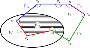
Figure 1: Illustration of the domains $\Omega$, $W$ and $W_{\delta}$.

$$W_{\delta}:=(W\cap\Omega)\setminus\bigcup_{i=1}^{n}\bar{B}(c_{i},\delta)$$

where the set $C=\{c_{i}\}_{i=1}^{n}$ of centers of balls with radius $\delta>0$ is introduced in the introduction.

Lemma 2.1.

The solution $y\in K$ of (2.1) with $u\in H^{1/2}(\Gamma_{U})$ satisfies

$$y\in H^{2}(W_{\delta})\cap C^{1,\lambda}(\bar{W}_{\delta})\quad\forall\lambda\in(0,\tfrac{1}{2})$$ (2.3)

for any $\delta>0$.

Proof.

We start with the proof of the property

$$\forall x\in\bar{W}_{\delta}\quad\exists\,\varepsilon_{x}>0:\quad y\in H^{2}(W_{\delta}\cap B(x,\varepsilon_{x}))$$ (2.4)

using localization arguments.

• If $x\in W_{\delta}$ we consider a ball $O_{x}=B(x,\varepsilon_{x})$ with $\varepsilon_{x}<\mathrm{dist}(x,\partial\Omega)$. The solution is harmonic in $O_{x}$ and hence even real analytic in $O_{x}$ [5, Theorem 1.7.1].

• For $x\in\Gamma_{D}\cap\bar{W}_{\delta}$ or $x\in\Gamma_{N}\cap\bar{W}_{\delta}$ we consider a neighborhood $O_{x}=B(x,\varepsilon_{x})\cap\Omega$ with $\varepsilon_{x}<\mathrm{dist}(x,C)$. Again, since the solution is harmonic in $O_{x}$ it is real analytic in $O_{x}$, [5, Theorem 2.7.1], i. e. near the smooth part of the Dirichlet or Neumann boundary.

• For the remaining case $x\in\Gamma_{S}\cap\bar{W}_{\delta}$ we fix a rotationally symmetric cut-off function $\eta\in\mathcal{D}(\mathbb{R}^{2})$ such that $\eta=1$ in a neighborhood of $x$ with a small support such that $\mathrm{supp}\,\eta\cap\Omega\subset W_{\delta/2}$, see the illustration in Figure 2.

  

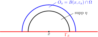
  Figure 2: Illustration of $\mathrm{supp}\,\eta$ and $O_{x}$.

  Let now $O_{x}=B(x,\varepsilon_{x})\cap\Omega$ with appropriately chosen $\varepsilon_{x}$ be a convex domain containing the support of $\eta$. Then $v=\eta w-\eta^{2}y+y$ with arbitrary

  $$w\in K_{x}:=\{z\in H^{1}(O_{x}):z\geq 0\ \text{on }\partial O_{x}\}$$

  satisfies $v=y=0$ on $\Gamma_{D}$ and $v=\eta w+(1-\eta^{2})y\geq 0$ on $\Gamma_{S}$ since all factors are greater than or equal to zero; hence $v\in K$. Inserting $v$ into (2.1) gives

  $$\int_{\Omega}\nabla y\cdot\nabla(\eta(w-\eta y))\geq\int_{\Gamma_{U}}u\eta(w-\eta y),$$

  and with $\eta\equiv 0$ in $\Omega\setminus O_{x}$ we get

  $$\int_{O_{x}}\nabla y\cdot\nabla(\eta(w-\eta y))\geq 0\quad\forall x\in K_{x}.$$ (2.5)

  Since $\partial_{n}\eta=0$ on $\partial O_{x}$ we get

  $$\int_{O_{x}} \nabla(\eta y)\cdot\nabla(w-\eta y)=\int_{O_{x}}(y\nabla\eta+\eta\nabla y)\cdot\nabla(w-\eta y)$$

  $$=-\int_{O_{x}}\nabla\cdot(y\nabla\eta)\cdot\nabla(w-\eta y)+\int_{O_{x}}\eta\nabla y\cdot\nabla(w-\eta y)$$

  $$=-\int_{O_{x}}\nabla\cdot(y\nabla\eta)(w-\eta y)+\int_{O_{x}}\nabla y\cdot\big{(}\nabla(\eta(w-\eta y))-\nabla\eta(w-\eta y)\big{)}$$

  $$\geq-\int_{O_{x}}\left(\nabla\cdot(y\nabla\eta)+\nabla y\cdot\nabla\eta\right)(w-\eta y)$$

  due to (2.5). Hence $\eta y\in K_{x}$ can be seen as the unique solution of

  $$\int_{O_{x}}(\nabla(\eta y)\cdot\nabla(w-\eta y)+\eta y(w-\eta y))\geq\int_{O_{x}}g_{x}(w-\eta y)\quad\forall w\in K_{x}$$

  with $g_{x}:=-\nabla\cdot(y\nabla\eta)-\nabla y\cdot\nabla\eta+\eta y\in L^{2}(O_{x})$. Grisvard and Iooss showed that $\eta y\in H^{2}(O_{x})$, see [10, Corollary 3.2].

Altogether the property (2.4) is proved.

The balls $B(x,\varepsilon_{x})$ form an open covering of $\bar{W}_{\delta}$, hence there exists a finite covering, i. e.,

$$\exists\,x_{j},\ j=1,\ldots,J:\quad\bar{W}_{\delta}\subset\bigcup_{j=1}^{J}B(x_{j},\varepsilon_{x_{j}}).$$

We conclude that

$$y\in H^{2}(W_{\delta})\subset W^{1,p}(W_{\delta})\quad\forall p\in[1,\infty).$$

With the same procedure as above we can now prove that $y\in C^{1,\lambda}(W_{\delta}\cap B(x,\varepsilon_{x}))$ for all $x\in\bar{W}_{2\delta}$. The point is that now $g_{x}\in L^{p}(O_{x})$ for all $p<\infty$ such that we can use a theorem from Khodja and Moussaoui, [14, Theorem 2] (see also [15]), to deduce that $\eta_{x}y$ belongs to $C^{1,\lambda}(O_{x})$ for all $\lambda\in(0,\frac{1}{2})$. As above we conclude $y\in C^{1,\lambda}(W_{2\delta})$. Since $\delta>0$ was arbitrary we are done. ∎

The following lemma is inspired from [11, §6], see also [14, Lemma III.1.3].

Lemma 2.2.

Denote by $\partial_{t}y$ and $\partial_{n}y$ the tangential and normal derivatives along the boundary. Then the equality

$$\partial_{t}y\,\partial_{n}y=0\ \text{on }\Gamma_{S}\setminus C.$$ (2.6)

holds.

Remark 2.3.

This result extends even to $\Gamma_{D}$ and $\Gamma_{N}$ since $\partial_{t}y=0$ on $\Gamma_{D}$ and $\partial_{n}y=0$ a.e. on $\Gamma_{N}$.

Proof.

Introduce the compact set

$$\Gamma_{S,\varrho}:=\Gamma_{S}\setminus\bigcup_{i=1}^{n}B(c_{i},\varrho)$$

for some $\varrho>0$. Then according to Theorem 2.1, $\partial_{n}y$ is continuous on $\Gamma_{S,\varrho}$, hence we can introduce the sets

$$\Gamma_{S,\varrho}^{+} =\{x\in\Gamma_{S,\varrho}\ |\ \partial_{n}y(x)>0\}, \Gamma_{S,\varrho}^{0} =\{x\in\Gamma_{S,\varrho}\ |\ \partial_{n}y(x)=0\},$$

and notice that $\Gamma_{S,\varrho}=\Gamma_{S,\varrho}^{+}\cup\Gamma_{S,\varrho}^{0}.$ At this stage, we distinguish two cases:

1. If $x\in\Gamma_{S,\delta}^{0}$, we have $\partial_{n}y(x)=0$ and hence

   $${\partial_{t}}y(x)\,\partial_{n}y(x)=0.$$ (2.7)

2. In the other case, $x\in\Gamma_{S,\delta}^{+}$, we have $y(x)=0$ due to the Signorini conditions. Observe that the continuity of $\partial_{n}y$ implies that $\Gamma_{S,\varrho}^{+}$ is an open subset of $\Gamma_{S,\varrho}$. Hence, if $x\in\Gamma_{S,\delta}^{+}$, then $y=0$ holds in a neighborhood of $x$, and the tangential derivative is also zero in this neighborhood and consequently $\partial_{t}y(x)=0$, which shows that (2.7) also holds in that case.

We have just shown that (2.7) is valid for all $x\in\Gamma_{S,\varrho}$ and letting $\varrho$ tend to zero we find (2.6). ∎

We prove now the main result of this section, namely the characterization of the coincidence set $\Gamma_{C}$, see (1.7). For that purpose, we adapt the method of Kinderlehrer in [11, §6] who treated the case of the elasticity system.

Theorem 2.4.

Let $y\in K$ be the unique solution of (2.1), then the coincidence set $\Gamma_{C}$ is the union of a finite numbers of intervals and finitely many isolated points.

Proof.

We localize the problem by considering a finite covering of $\Gamma_{S}$. Introduce a finite number of open balls $B(c_{i},\varrho_{i})$, $i\in J$. The index set $J$ is chosen such that $J\supset\{i\in C:x_{i}\in\bar{\Gamma}_{S}\}$ and the radii $\varrho_{i}>0$ are chosen such that $\Gamma_{S}\subset\bigcup_{i\in J}B(c_{i},\varrho_{i})$ and $c_{j}\not\in B(c_{i},\varrho_{i})$ for $i\neq j$, see Figure 3. Note that the index set may contain further points $c_{i}\in\Gamma_{S}\setminus C$.

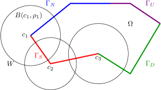
Figure 3: Illustration of the domain, the boundary conditions and the covering.

We consider now any ball $B(c_{i},\varrho_{i})$ and omit the index $i$ for better readability. Introduce a local polar coordinate system $(r,\theta)$ centered in $c$, such that

$$O_{\alpha}:=B(c,\varrho)\cap\Omega=\{(r\cos\theta,r\sin\theta)\in\mathbb{R}^{2}:0<r<\varrho,0<\theta<\alpha\}$$

where $\alpha$ is the angle of the domain at $c$. Consider now the situation where

$$\Gamma_{0}:=\{(r\cos\theta,r\sin\theta)\in\mathbb{R}^{2}:0<r<\varrho,\theta=0\}\subset\Gamma_{S}.$$

The other leg $\Gamma_{\alpha}:=\{(r\cos\theta,r\sin\theta)\in\mathbb{R}^{2}:0<r<\varrho,\theta=\alpha\}$ may be contained in $\Gamma_{D}$, $\Gamma_{N}$ or $\Gamma_{S}$ but not in $\Gamma_{U}$ because of $\bar{\Gamma}_{S}\cap\bar{\Gamma}_{U}=\emptyset$, see (1.6). Note that the situation where $\Gamma_{\alpha}\subset\Gamma_{S}$ and $\Gamma_{0}\not\subset\Gamma_{S}$ can be treated in a similar way.

The function $y$ satisfies

$$-\Delta y =0\quad\text{in }O_{\alpha},$$

$$y\geq 0,\ \partial_{n}y\geq 0,\ y\partial_{n}y =0\quad\text{on }\Gamma_{S}\cap B(c,\varrho).$$

Now regarding $y$ as a function of the complex variable $z=x_{1}+\mathrm{i}\,x_{2}$, we define the function

$$w(z)=\partial_{2}y(z)+\mathrm{i}\,\partial_{1}y(z),$$

defined in $O_{\alpha}$ (now considered as a subset of $\mathbb{C}$), see the illustration in Figure 4.

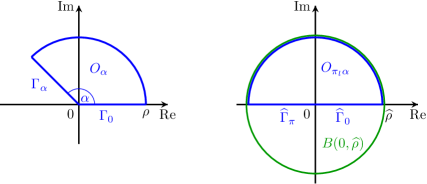
Figure 4: Illustration of transformation.

As $y$ is harmonic in $O_{\alpha}$ and belongs to $C^{2}(O_{\alpha})$, the function $w$ is analytic in $O_{\alpha}$, [4, p. 41]. Furthermore, we introduce the biconformal mapping

$$h:z\mapsto\hat{z}=z^{\pi/\alpha},\quad O_{\alpha}\to O_{\pi,\alpha}:=\{z=r\mathrm{e}^{\mathrm{i}\,\theta}\in\mathbb{C}:0<r<\varrho^{\pi/\alpha},0<\theta<\pi\},$$

and denote $\hat{\Gamma}_{0}:=h(\Gamma_{0})$ and $\hat{\Gamma}_{\pi}:=h(\Gamma_{\alpha})$. Note the simple rule

$$h:r\mathrm{e}^{\mathrm{i}\,\theta}\mapsto\hat{r}\mathrm{e}^{\mathrm{i}\,\hat{\theta}}\quad\text{with }\hat{r}=r^{\pi/\alpha}\text{ and }\hat{\theta}=\frac{\theta\pi}{\alpha}.$$

Let us analyze now the function

$$\hat{y}(\hat{z}):=y(z).$$

Since a conformal mapping preserves the Laplace operator (up to a factor) and since the normal derivative is up to a factor again the $\theta$-derivative we get

$$-\Delta\hat{y} =0\quad\text{in }O_{\pi,\alpha},$$

$$\hat{y}\geq 0,\quad\hat{\partial}_{n}\hat{y}\geq 0,\quad\hat{y}\hat{\partial}_{n}\hat{y} =0\quad\text{on }\hat{\Gamma}_{0},$$

and the appropriate Dirichlet, Neumann or Signorini boundary condition on $\hat{\Gamma}_{\pi}$. Moreover, we can compute

$$\partial_{r}y =\partial_{r}\hat{r}\,\partial_{\hat{r}}\hat{y}=\tfrac{\pi}{\alpha}r^{\pi/\alpha-1}\partial_{\hat{r}}\hat{y}, \partial_{\theta}y =\partial_{\theta}\hat{\theta}\,\partial_{\hat{\theta}}\hat{y}=\tfrac{\pi}{\alpha}\partial_{\hat{\theta}}\hat{y},$$

such that

$$\int_{O_{\pi,\alpha}}|\hat{\nabla}\hat{y}|^{2} =\int_{O_{\pi,\alpha}}\left(|\partial_{\hat{r}}\hat{y}|^{2}+|\hat{r}^{-1}\partial_{\hat{\theta}}\hat{y}|^{2}\right)\,\hat{r}\mathrm{d}\hat{r}\mathrm{d}\hat{\theta}$$

$$=\int_{O_{\alpha}}\left((\tfrac{\pi}{\alpha})^{-2}r^{2(1-\pi/\alpha)}|\partial_{r}y|^{2}+r^{-2\pi/\alpha}(\tfrac{\pi}{\alpha})^{-2}|\partial_{\theta}y|^{2}\right)\,r^{\pi/\alpha}\,\tfrac{\pi}{\alpha}r^{\pi/\alpha-1}\mathrm{d}r\,\tfrac{\pi}{\alpha}\mathrm{d}\theta$$

$$=\int_{O_{\alpha}}\left(|\partial_{r}y|^{2}+|r^{-1}\partial_{\theta}y|^{2}\right)\,r\mathrm{d}r\mathrm{d}\theta=\int_{O_{\alpha}}|\nabla y|^{2},$$

i. e., for the function

$$\hat{w}(\hat{z}):=\partial_{1}\hat{y}+\mathrm{i}\,\partial_{2}\hat{y}$$

the relation

$$|\hat{w}(\hat{z})^{2}| =|\hat{w}(\hat{z})|^{2}=|\hat{\nabla}\hat{y}|^{2}\in L^{1}(O_{\pi,\alpha})$$

holds.

Lemma 2.2 and Remark 2.3 imply that

$$\Im\left(w(z)\right)^{2}=0\hbox{ on }(-\hat{\varrho},\hat{\varrho})\setminus\{0\},$$

with $\hat{\varrho}=\varrho^{\pi/\alpha}$. Consequently on $U:=B(0,\hat{\varrho})\setminus\{0\}$, we define the function

$$F(z)=\begin{cases}w(z)^{2}&\hbox{ if }\Im z\leq 0,\\[2.15277pt] \overline{w(\bar{z})^{2}}&\hbox{ if }\Im z>0,\end{cases}$$

which is analytic in $U$ by the Schwarz reflection principle, see [4, §IX.1]. Hence $F$ is meromorphic in $U$. As additionally $F$ belongs to $L^{1}(U)$ we conclude that $F$ admits the Laurent expansion

$$F(z)=\frac{c}{z}+F_{H}(z),$$

with $c\in\mathbb{C}$ and a function $F_{H}$ which is an analytic in $B(0,\hat{\varrho})$. (Terms $z^{-j}$ with $j>1$ are not in $L^{1}(U)$.) This implies that the function

$$\Phi(z)=zF(z)$$

is holomorphic on $B(0,\hat{\varrho})$. Therefore $\Phi$ has a finite number of zeroes on $\hat{\Gamma}:=\{z\in\bar{U}:\Im z=0\}$ if $\Phi$ is not identically equal to 0.

Let us analyze two cases:

1. If $\Phi$ is identically equal to 0, then by (2.6) we get

   $$w(z)^{2}=(\partial_{2}y)^{2}-(\partial_{1}y)^{2}=0\hbox{ on }\hat{\Gamma}\setminus\{0\},$$

   which again by (2.6) implies

   $$\partial_{2}y=\partial_{1}y=0\hbox{ on }\hat{\Gamma}\setminus\{0\}.$$

   Consequently $y$ is constant on $\hat{\Gamma}$, so either this constant is zero and $\hat{\Gamma}_{C}:=\{z\in\hat{\Gamma}:\hat{y}(z)=0\}=\hat{\Gamma}$, or this constant is different from zero and $\hat{\Gamma}_{C}=\emptyset$.

2. If $\Phi$ is not identically equal to 0, the sets $\{z\in\hat{\Gamma}:\Phi(z)>0\}$ and $\{z\in\hat{\Gamma}:\Phi(z)<0\}$ are unions of a finite number of intervals $I$. We are looking for the behavior of $y$ on any of these intervals $I$. Depending on the sign of $z\in\hat{\Gamma}$ we find that $\Phi(z)=zF(z)$ is positive or negative in $I$, hence $(\partial_{2}y)^{2}-(\partial_{1}y)^{2}$ does not change sign in $I$, and moreover $(\partial_{2}y)^{2}>0$ or $(\partial_{1}y)^{2}>0$ in $I$. If $(\partial_{2}y(z))^{2}>0$ then we get by the Signorini condition that $y\equiv 0$ in $I$. If $(\partial_{1}y(z))^{2}>0$ then the function $y$ is nowhere constant in $I$, hence $y$ has no or a finite number of zeros in $I$, and we get by the Signorini condition that $\partial_{n}y=0$ a.e. in $I$.

In conclusion, in this case $\hat{\Gamma}_{C}$ is the union of a finite number of intervals plus eventually a finite number of points. Since the mapping $h$ is continuous this result is valid also for $\Gamma_{C}$. ∎

Remark 2.5.

Let us finish this section with a discussion of our assumption that we assumed a homogeneous differential equation in (1.1) and a homogeneous gap function in (1.5).

• The assumption of a homogeneous differential equation in (1.1) was made to simplify the discussion. For Lemma 2.1 a right hand side $f\in L^{\infty}(\Omega)$ could be admitted. Recall also the introduction of the domain $W$ in (2.2). The whole analysis is untouched if the equation is homogeneous in a neighborhood of $\Gamma_{S}$ only since then the set $W$ could be defined accordingly.

• In particular cases the solution of non-homogeneous problem could be homogenized. Assume that the differential equation in (1.1) is replaced by $-\Delta y=f$ and the gap condition in (1.5) is replaced by $y\geq\psi$. If $f$ and $\psi$ are such that there exists a function $y_{f,\psi}$ such that

  $$-\Delta y_{f,\psi} =f\quad\text{in }\Omega,$$

  $$y_{f,\psi} =0\quad\text{on }\Gamma_{D},$$

  $$\partial_{n}y_{f,\psi} =0\quad\text{on }\Gamma_{N}\cup\Gamma_{U},$$

  $$y_{f,\psi}=\psi,\ \partial_{n}y_{f,\psi} =0\quad\text{on }\Gamma_{S},$$

  then $y-y_{f,\psi}$ satisfies our assumptions. Of course this problem is overdetermined such that the existence of a solution cannot be expected for any $f$ and $\psi$. But examples can be constructed by choosing a function

  $$y_{*}\in\{v\in H^{2}(\Omega):v=0\text{ on }\Gamma_{D},\partial_{n}v=0\text{ on }\Gamma_{N}\cup\Gamma_{U}\cup\Gamma_{S}\}\supset H^{2}_{0}(\Omega)$$

  and defining $f=-\Delta y_{*}$ and $\psi=y_{*}|_{\Gamma_{S}}$.

Example 2.6.

Christof and Haubner investigated in [3] a square domain and the case $\Gamma=\Gamma_{S}$. In the case of a homogeneous differential equation, Condition (A) in this paper is now proven in Theorem 2.4, namely that the relative boundary of $\Gamma_{C}$ has one-dimensional Hausdorff measure zero and the relative interior of $\Gamma_{C}$ consists of at most finitely many connected components.

3 Regularity of the solution

We formulate now a regularity result in the spirit of Theorem 2.3 of the paper [3] by Christof and Haubner where the regular part of the solution is considered in $W^{2,p}$, $p>2$, $p\not=4$. But we like to note that the regular part could also be smoother; the prize is that possibly more singular terms have to be included and the datum $u$ at the Neumann boundary must be sufficiently regular.

Theorem 3.1.

Let $y$ be the solution of problem (1.1)–(1.5). Recall the set $\{c_{i}\}_{i=1}^{n}$ of critical points and the interior angles $\alpha_{i}$. Recall also that there are points $\{c_{i}\}_{i=n+1}^{m}\subset\Gamma_{S}\setminus C$ of unknown location which are the endpoints of the intervals in the coincidence set and in that case, set $\alpha_{i}=\pi$. Furthermore denote by $(r_{i},\theta_{i})$ local polar coordinates at all these points.

Let $p>2$, $p\not\in P$, where the finite set $P$ of exceptional values is a subset of the countable set

$$\left\{\frac{2}{2-\frac{k\pi}{2\alpha_{i}}},\ k\in\mathbb{N},\ i=1,\ldots,m\right\}.$$

Assume that $u\in W^{1-1/p,p}(\Gamma_{U})$ satisfies the compatibility condition $u(c_{i})=0$

• if $c_{i}\in\bar{\Gamma}_{D}\cap\bar{\Gamma}_{U}$ and $\alpha_{i}=\frac{1}{2}\pi$ or $\alpha_{i}=\frac{3}{2}\pi$ or

• if $c_{i}\in\bar{\Gamma}_{N}\cap\bar{\Gamma}_{U}$ and $\alpha_{i}=\pi$.

Then there is a representation of $y$

$$y=y_{R}+\sum_{i=1}^{n}\sum_{j:0<\lambda_{i,j}<2-2/p\atop\lambda_{i,j}\neq 1}d_{i,j}r_{i}^{\lambda_{i,j}}\Phi_{i,j}(\theta_{i})+\sum_{i=n+1}^{m}d_{i}r_{i}^{3/2}\Phi_{i}(\theta_{i})$$

with $y_{R}\in W^{2,p}(\Omega)$, coefficients $d_{i,j}$ and $d_{i}$, smooth functions $\Phi_{i,j}$ and $\Phi_{i}$, and exponents

$$\lambda_{i,j}=\begin{cases}j\pi/\alpha_{i}&\text{if D-D or N-N or U-U or U-N conditions near }c_{i},\quad j\geq 1,\\ (j-\frac{1}{2})\pi/\alpha_{i}&\text{if D-N or D-U conditions near }c_{i},\quad j\geq 1,\\ j\pi/(2\alpha_{i})&\text{if S-S conditions near }c_{i},\quad j\geq 2,\\ j\pi/(2\alpha_{i})&\text{if S-D or S-N conditions near }c_{i},\quad j\geq 1,\end{cases}$$

where D-N means that one boundary edge at $c_{i}$ is contained in $\Gamma_{D}$ and the other in $\Gamma_{N}$, and so on.

Remark 3.2.

The compatibility conditions could be omitted, but then a singularity of the form $r(\Phi_{1}(\theta)+\log r\Phi_{2}(\theta))$ with $\Phi_{i}$ smooth has to be added, see [9, p. 263].

Proof.

Since we have a finite number of critical boundary points $c_{i}$ due to Theorem 2.4 we can treat them separately and use classical theory as described for instance in [9, Corollary 4.4.4.14]. Let us discuss shortly the situation near the Signorini boundary.

For $i\leq n$ and $c_{i}\in\bar{\Gamma}_{S}\cap\bar{\Gamma}_{D}$ or $c_{i}\in\bar{\Gamma}_{S}\cap\bar{\Gamma}_{N}$ we do not know whether a Dirichlet or Neumann boundary condition occurs on $\Gamma_{S}$ near $c_{i}$. Therefore we consider the worst situation of mixed boundary conditions.

In the remaining cases some singularities disappear at $c_{i}\in\bar{\Gamma}_{S}$:

1. For $i=n+1,\ldots,m$ the leading singularity is $r_{i}^{3/2}$ since the term $r_{i}^{1/2}$ is not in $H^{2}(\Omega)$, compare the result in Lemma 3.1, and see the discussion in e. g. [3, 14].

2. For $i\leq n$ and $c_{i}\in\Gamma_{S}$ the worst situation could be mixed. Let us consider the case that Dirichlet conditions is valid for $\theta_{i}=0$. Then we have in the vicinity of $c_{i}$

   $$y=y_{r}+dr_{i}^{\pi/(2\alpha_{i})}\sin\left(\frac{\pi\theta_{i}}{2\alpha_{i}}\right).$$ (3.1)

   We show now $y_{r}=o(r_{i}^{\pi/(2\alpha_{i})})$ such that this term is neglectable sufficiently close to $c_{i}$. Indeed from [9, Corollary 4.4.4.14] near $c_{i}$, we have

   $$y_{r}=y_{R}+\sum_{j\in\mathbb{N}\setminus\{0\}:0<(j+1/2)\pi/\alpha_{i}<2-2/p\atop(j+1/2)\pi/\alpha_{i}\neq 1}d_{i,j}r_{i}^{(j+1/2)\pi/\alpha_{i}}\sin((j+1/2)\pi\theta_{i}/\alpha_{i}),$$ (3.2)

   with $y_{R}\in W^{2,p}(\Omega\cap B(c_{i},\rho))$ for $\rho$ small enough and $d_{i,j}\in\mathbb{R}$. Consequently, near $c_{i}$,

   $$y_{R}(r_{i},0)=0,\quad\frac{\partial y_{R}}{\partial\theta_{i}}(r_{i},\alpha_{i})=0\quad\forall r_{i}<\rho.$$ (3.3)

   Notice that the Sobolev embedding theorem guarantees that

   $$y_{R}\in C^{1,\beta}(\bar{\Omega}\cap\bar{B}(c_{i},\rho))\ \text{with }\beta=1-2/p.$$ (3.4)

   We now notice that the second term in the sum in (3.2) (if any) is trivially $o(r_{i}^{\pi/(2\alpha_{i})})$, hence it remains to check the same behavior for $y_{R}$. We note that $\nabla y_{R}(c_{i})=0$ except in the cases $\alpha_{i}=\frac{1}{2}\pi$ or $\alpha_{i}=\frac{3}{2}\pi$, and that $r_{i}^{(j+1/2)\pi/\alpha_{i}}$ is smooth when $\alpha_{i}=\frac{1}{2}\pi$. For that purpose, we distinguish three cases.

   1. If $\pi/(2\alpha_{i})<1$, then by Taylor’s theorem (and since $y_{R}(c_{i})=0$), we have

      $$y_{R}(x)=\nabla y_{R}(c_{i})\cdot(x-c_{i})+o(r_{i}),$$

      which yields $y_{R}(x)=O(r_{i})=o(r_{i}^{\pi/(2\alpha_{i})})$ as $\pi/(2\alpha_{i})<1$.

   2. If $\pi/(2\alpha_{i})=1$, then from [9, Corollary 4.4.4.14], we directly have

      $$y=y_{R}\in W^{2,p}(\Omega\cap B(c_{i},\rho)),$$

      in other words the singular part is zero.

   3. If $\pi/(2\alpha_{i})>1$, then owing to (3.3) and the regularity of $y_{R}$, we actually have

      $$\nabla y_{R}(c_{i})=0,$$

      hence by Taylor’s expansion with an integral remainder, we have

      $$y_{R}(x)=\int_{0}^{1}\nabla y_{R}(c_{i}+t(x-c_{i}))(x-c_{i})\,dt,\forall|x-c_{i}|<\rho.$$

      Therefore as $|\nabla y_{R}(c_{i}+t(x-c_{i}))|=|\nabla y_{R}(c_{i}+t(x-c_{i}))-\nabla y_{R}(c_{i})|=O((tr_{i})^{\beta})$ due to (3.4), one deduces that

      $$|y_{R}(x)|=O(r_{i}^{\beta+1})=o(r_{i}^{\pi/(2\alpha_{i})}),$$

      as $\pi/(2\alpha_{i})<\beta+1$. (In the case $\pi/(2\alpha_{i})>\beta+1=2-2/p$ the solution $y$ is $W^{2,p}$-regular in the vicinity of $c_{i}$. Equality is excluded by assumption.)

   Coming back to (3.1), for $\theta_{i}=0$ we get $\partial_{n}y=\partial_{n}y_{r}-dr_{i}^{\pi/(2\alpha_{i})-1}$, hence $d\leq 0$ in order to satisfy the Signorini condition $\partial_{n}y\geq 0$. For $\theta_{i}=\alpha_{i}$ we get $y=y_{r}+dr_{i}^{\pi/(2\alpha_{i})}$, hence $d\geq 0$ in order to satisfy the Signorini condition $y\geq 0$. So we can have only $d=0$.

Since all cases are treated the proof is complete. ∎

Example 3.3.

Let us shortly discuss the L-domain; that is a hexahedron with one interior angle $\alpha=\frac{3}{2}\pi$ and all others being of size $\frac{1}{2}\pi$. The leading singular term near the non-convex corner is of type $r^{\lambda}$ with $\lambda=\frac{2}{3}$ if Signorini conditions are given at both legs of this angle, but with $\lambda=\frac{1}{3}$ if a Signorini condition is given on one leg only, and a Dirichlet or Neumann condition at the other leg. These terms are in $H^{s}(\Omega)$ for $s<1+\lambda$ or in a suitable weighted Sobolev space. The set of exception values for $p$ is $P=\{3,6\}$.

Acknowledgment

The authors thank Constantin Christof for pointing to an incorrect argument in a previous version of the paper. The authors thank also Christof Haubner for preparing the illustrations.

References

- [1] Z. Belhachmi and F. B. Belgacem. Quadratic finite element approximation of the Signorini problem. Math. Comp., 72(241):83–104, 2003.
- [2] H. Brézis. Monotonicity methods in Hilbert spaces and some applications to nonlinear partial differential equations. In Contributions to nonlinear functional analysis (Proc. Sympos., Math. Res. Center, Univ. Wisconsin, Madison, Wis., 1971), pages 101–156, 1971.
- [3] C. Christof and C. Haubner. Finite element error estimates in non-energy norms for the two-dimensional scalar signorini problem. Preprint IGDK-2018-14, IGDK 1754, TU München, 2018. https://www.igdk.eu/foswiki/pub/IGDK1754/Preprints/Christof_SignoriniNitscheTrick.pdf.
- [4] J. B. Conway. Functions of one complex variable, volume 11 of Graduate Texts in Mathematics. Springer-Verlag, New York-Berlin, second edition, 1978.
- [5] M. Costabel, M. Dauge, and S. Nicaise. Corner Singularities and Analytic Regularity for Linear Elliptic Systems. Part I: Smooth domains. HAL report hal-00453934, 2010. https://hal.archives-ouvertes.fr/hal-00453934.
- [6] G. Drouet and P. Hild. Optimal convergence for discrete variational inequalities modelling Signorini contact in 2D and 3D without additional assumptions on the unknown contact set. SIAM J. Numer. Anal., 53(3):1488–1507, 2015.
- [7] G. Fichera. Unilateral constraints in elasticity. In Actes du Congrès International des Mathématiciens (Nice, 1970), Tome 3, pages 79–84. 1971.
- [8] R. Glowinski, J.-L. Lions, and R. Trémolières. Numerical analysis of variational inequalities, volume 8 of Studies in Mathematics and its Applications. North Holland, Amsterdam, New York, 1981. Translated from the French.
- [9] P. Grisvard. Elliptic problems in nonsmooth domains, volume 24 of Monographs and Studies in Mathematics. Pitman, Boston–London–Melbourne, 1985.
- [10] P. Grisvard and G. Iooss. Problèmes aux limites unilatéraux dans des domaines non réguliers. In Publications des Séminaires de Mathématiques, Université de Rennes, pages 1–26, Rennes, 1975.
- [11] D. Kinderlehrer. Remarks about Signorini’s problem in linear elasticity. Ann. Scuola Norm. Sup. Pisa Cl. Sci. (4), 8(4):605–645, 1981.
- [12] D. Kinderlehrer. The smoothness of the solution of the boundary obstacle problem. J. Math. Pures Appl. (9), 60(2):193–212, 1981.
- [13] D. Kinderlehrer and G. Stampacchia. An introduction to variational inequalities and their applications, volume 88 of Pure and Applied Mathematics. Academic Press, Inc. [Harcourt Brace Jovanovich, Publishers], New York-London, 1980.
- [14] M. Moussaoui and K. Khodja. Régularité des solutions d’un problème mêlé Dirichlet-Signorini dans un domaine polygonal plan. Comm. Partial Differential Equations, 17(5-6):805–826, 1992.
- [15] N. N. Uraltseva. On the regularity of solutions of variational inequalities. Uspekhi Mat. Nauk, 42(6(258)):151–174, 248, 1987.
- [16] B. I. Wohlmuth, A. Popp, M. W. Gee, and W. A. Wall. An abstract framework for a priori estimates for contact problems in 3D with quadratic finite elements. Comput. Mech., 49(6):735–747, 2012.