Fluctuations and Correlations in a Model of Extreme Introverts and Extroverts

Abstract

Unlike typical phase transitions of first and second order, a system displaying the Thouless effect exhibits characteristics of both at the critical point (jumps in the order parameter and anomalously large fluctuations). An $extreme$ Thousless effect was observed in a recently introduced model of social networks consisting of ‘introverts and extroverts’ ($XIE$). We study the fluctuations and correlations of this system using both Monte Carlo simulations and analytic methods based on a self-consistent mean field theory. Due to the symmetries in the model, we derive identities between all independent two point correlations and fluctuations in three quantities (degrees of individuals and the total number of links between the two subgroups) in the stationary state. As simulations confirm these identities, we study only the fluctuations in detail. Though qualitatively similar to those in the 2D Ising model, there are several unusual aspects, due to the extreme Thouless effect. All these anomalous fluctuations can be quantitatively understood with our theory, despite the mean-field aspects in the approximations. In our theory, we frequently encounter the ‘finite Poisson distribution’ (i.e., $x^{n}/n!$ for $n\in\left[0,N\right]$ and zero otherwise). Since its properties appear to be quite obscure, we include an Appendix on the details and the related ‘finite exponential series’ $\sum_{0}^{N}x^{n}/n!$. Some simulation studies of joint degree distributions, which provide a different perspective on correlations, have also been carried out.

I Introduction

For systems undergoing phase transition, the study of fluctuations and correlations usually offer insight into the underlying collective behavior of the constituents. Such studies are especially important for typical second order transitions, where large, anomalous, and non-analytic properties emerge. Somewhat outside the conventional wisdom of critical phenomena are ‘mixed order transitions,’ also known as the Thouless effect. Displaying characteristics of both a first order transition (e.g., jumps in the order parameter) and a second order one (e.g., anomalously large fluctuations), this effect has been studied continuously kafri_why_2000 ; poland_phase_1966 ; fisher_effect_1966 since fifty years ago, when Thouless’ introduction of the inverse distance squared Ising model Thouless_long-range_1969 . More recently, Bar and Mukamel BarMukamel coined the term ‘extreme Thouless effect’ (ETE) for a system that displays maximal jumps (e.g., $-1$ magnetisation to $+1$ across the transition) and ‘infinite’ fluctuations (i.e., variations scaling with the whole system) at the transition itself.

Though the ETE effect seems exotic, a natural route exists for constructing an arguably trivial (and exactly solvable) system which displays it. Introduced in the context of a kinetic Ising model FFK16 , it is best viewed as a static system with a special Hamiltonian. Consider the non-interacting Ising model with $\mathcal{N}$ spins ($s_{\alpha}=\pm 1$) in an external field, $H$, at inverse temperature $\beta=1$. Thus $P\left(M\right)$, the exact probability for finding the system with a given total magnetisation $M$, is proportional to a binomial times $e^{HM}$, while the Landau free energy, $-k_{B}T\ln P$, is $\ln\frac{\mathcal{N}+M}{2}!+\ln\frac{\mathcal{N-}M}{2}!-HM$ (apart from a const). All we needed to produce a ETE is to introduce an interaction Hamiltonian which cancels the first two terms here, i.e., $\mathcal{H}\left(\left\{s_{i}\right\}\right)=-\ln\left[\left(\mathcal{N}+\sum_{\alpha}s_{\alpha}\right)/2\right]!-\ln\left[\left(\mathcal{N-}\sum_{\alpha}s_{\alpha}\right)/2\right]!$. Now, the free energy (at $\beta=1$) is just $-HM$. Restricted to $m\equiv M/\mathcal{N}\in\left[-1,1\right]$, the minimum is located at $sign\left(H\right)$, so that $m$ literally jumps from $-1$ to $+1$ when $H$ crosses $0$. Meanwhile, at $H=0$, $P$ is completely flat over the entire interval. Despite such drastic displays, there is no correlation between any pair of spins. In this paper, we will explore a less trivial system which displays the ETE, and in particular, the non-vanishing correlations between its constituents.

The model system we study consists of a network of dynamic links, motivated by the changing contacts between individuals in a social settingliu2013modeling . In a typical population, we can expect to find a range of preferences for how many contacts seems best, e.g., introverts preferring few and extroverts, many. Labeling a node (an individual) by $i$ and its preferences by $\kappa_{i}$, we evolve our simple model by choosing a node at random and noting its degree $k_{i}$ – the number of links (contacts) it has. If $k_{i}<\kappa_{i}$, it chooses another node (which is not already in contact) at random and makes a link to that. Otherwise, it chooses a random existing link and cuts it. At any time, this social network is completely described by the adjacency matrix $\mathbb{A}$, the elements of which are binary: $a_{ij}=a_{ji}=1$ (or $0$) if the link between nodes $i$ and $j$ is present (or absent). Thus, the evolution of our system resembles that of a special kinetic two dimensional (2D) Ising model, in which a pair of spins ($s_{ij}=2a_{ij}-1=s_{ji}$) can be flipped in each step, depending on how many other spins in the same row (or column) are the same. In general, the dynamics of such a system do not obey detailed balanceliu2013modeling , so that the system eventually settles into a non-equilibrium steady state (NESS), characterized by a stationary distribution, $\mathcal{P}^{\ast}\left(\mathbb{A}\right)$, as well as persistent probability currents, $\mathcal{K}^{\ast}\left(\mathbb{A\rightarrow A}^{\prime}\right)$ zia2007probability . Needless to say, understanding the collective behavior of this system is extremely challenging and so, only some simpler versions have been studied in detail so far. Notable examples are (a) a homogeneous population, with just one $\kappa$ for all liu2013modeling , (b) a population with $N_{I}$ ‘introverts’ and $N_{E}$ ‘extroverts,’ specified by $\kappa_{I}<\kappa_{E}$ liu2014modeling , and most extensively, (c) the $XIE$ model zia2012extraordinary ; liu2013extraordinary ; bassler2015extreme ; bassler2015networks ; ZZEB2018 for the extreme case of the latter, with $\kappa_{I}=0$ and $\kappa_{E}=\infty$. In particular, the ETE was found in the last case zia2012extraordinary ; liu2013extraordinary . Beyond these models with static $\kappa$’s, the further motivation is to exploit adaptive networks, in which the preference may be dynamic due to personal reasons or external controls, to model realistic social phenomena such as revelation of hidden secrets or response to epidemicsplatini2010 ; jolad2012 .

This paper reports the continuing study of the $XIE$ model. Specifically, despite the apparent presence of long-ranged and multi-spin interactionszia2012extraordinary ; liu2013extraordinary , mean field approximations (MFA) have been extraordinarily successful in capturing all aspects of the ETEbassler2015extreme ; bassler2015networks ; ZZEB2018 . A series of natural questions thus arises: What is the nature of the correlations? Are they small, so that the MFAs are so effective? Given that intimate relations exist between correlations and fluctuations, how can they be small when the fluctuations are ‘extreme’ at the critical point? Before attempting to answer these questions, we provide details of the model in the next Section, as well as the similarities and contrasts with the standard 2D Ising model. Turning to fluctuations and correlations in the following Section, we display the identities which relate fluctuations of magnetisation-like quantities to the standard two-point correlations, and we introduce another measure of correlations which is natural for networks but not for Ising systems. Stimulation data and various mean-field approaches will be presented next. Much of the theory is based on finite Poisson distributions, with somewhat unusual properties. Since they appear to be rarely discussed in the literature, we include a substantial section in the Appendix on the results we derived. We end with a summary and outlook.

II The $XIE$ model and connections to the Ising model

The dynamic network we study here, the $XIE$ model, is an extreme version of social connections between $N_{I}$ introverts ($I$’s) and $N_{E}$ extroverts ($E$’s). The system evolves in discrete time steps: At each step, one of the $N_{I}+N_{E}$ nodes is randomly chosen to act. If an $I$ with $k$ ($>0$) links is chosen, it will cut one of the links with probability $1/k$. If an $E$ with no connections to $p$ others is chosen, it will make a connection to one of these with probability $1/p$. Since no $I$ makes links and no $E$ cuts them, it is clear that, starting with any initial network, this minimal system will quickly settle into two distinct subgroups: $I$’s with no links amonst themselves and a complete graph of all the $E$’s. The only dynamic links are the cross links between these groups and in this sense, the fluctuating part of our network ranges over all the bipartite graphs. Thus, we only need to focus on one of the off diagonal blocks of the adjacency matrix $\mathbb{A}$, i.e., the incidence matrix $\mathbb{N}$. Let us denote the elements of $\mathbb{N}$ by $n_{i\eta}$, with $i=1,...,N_{I}$ and $\eta=1,...,N_{E}$, which assumes the values $1$ and $0$ if the link between introvert $i$ and extrovert $\eta$ is present or absent, respectively. In the sense that $n$ is an occupation variable, we will also use the language of particle/hole for these states. A typical configuration of an $N_{I,E}=5,4$ system in its steady state is illustrated in Fig.1, for which we have

$$\mathbb{N}=\left(\begin{array}[]{cccc}0&0&0&1\\ 1&0&1&0\\ 0&1&0&0\\ 0&1&0&0\\ 0&0&1&0\end{array}\right)$$

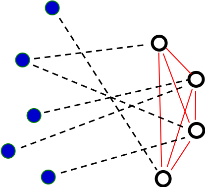
Figure 1: A typical steady state configuration of an $N_{I,E}=5,4$ system. The $I$’s are represented as solid (blue on line) circles while $E$’s are open ones. The $i$,$\eta$ labels nodes from top to bottom. All $I$-$I$ ($E$-$E$) links are absent (present, solid lines, red on line), while only the $I$-$E$ links (dashed lines) are dynamic.

Although our focus here will be much more modest, the ultimate goal of the statistical mechanics of $XIE$ model is the solution to the master equation for the probability distribution

$$\mathcal{P}\left(\mathbb{N};t+1\right)-\mathcal{P}\left(\mathbb{N};t\right)=\sum_{\mathbb{N}^{\prime}}\mathbb{\mathcal{L}}\left(\mathbb{N\leftarrow N}^{\prime}\right)\mathcal{P}\left(\mathbb{N}^{\prime};t\right)$$

which governs the evolution of $\mathbb{N}$ in discrete time, given an initial distribution $\mathcal{P}\left(\mathbb{N};0\right)$. Here, $\mathcal{L}$ is known as the Liouvillian and plays the role of the Hamiltonian in the Schrödinger equation. It is composed of the transition probabilities (from $\mathbb{N}^{\prime}$ to $\mathbb{N}$) and, since its explicit form is quite involved but not relevant, will not be discussed further. Nevertheless, we emphasize that it is known to obey detailed balance zia2012extraordinary ; liu2013extraordinary and so, the system eventually settles into an equilibrium stationary state with distribution $\mathcal{P}^{\ast}\left(\mathbb{N}\right)\propto\Pi_{i}\left(k_{i}!\right)\Pi_{\eta}\left(p_{\eta}!\right)$ (and zero persistent probability currents zia2007probability ). Here,

$$k_{i}=\sum_{\eta}n_{i\eta};~{}~{}p_{\eta}=N_{I}-\sum_{i}n_{i\eta}$$

denote, respectively, the particle and hole content of a row and column. Note that $k_{i}$ and $\left(N_{I}-p_{\eta}\right)$ are just the degrees of nodes $i$ and $\eta$. Since an $I$ ($E$) prefers to have no links (links to all), $k$ ($p$) is a measure of the ‘frustration’ of the node. Finally, given that $\mathcal{P}^{\ast}$ is like a Boltzmann factor, we may regard

$$\mathcal{H}\left(\mathbb{N}\right)=-\sum_{i}\ln\left(k_{i}!\right)-\sum_{\eta}\ln\left(p_{\eta}!\right)$$ (1)

as a Hamiltonian (with inverse temperature $\beta=1$ in this case).

As with $\mathbb{A}$ above, $\mathbb{N}$ can be regarded as a 2-D Ising model in the lattice gas representation. Unlike $\mathbb{A}$, which must remain symmetric to model undirected links in a network, there are no constraints on $\mathbb{N}$, so that the dynamics involve only single ‘spin’ flips. Of course, there are major differences between $XIE$ model and the Ising, some of which are listed here. The only (explicit) control parameters in our minimal model are $N_{I,E}$. While $\mathcal{N\equiv}N_{I}N_{E}$ corresponds to the overall system size of the Ising model, the aspect ratio, $N_{I}/N_{E}$, is rarely considered as a variable. Alternatively, we often use the average and difference

$$N\equiv\left(N_{I}+N_{E}\right)/2;~{}~{}\Delta\equiv N_{E}-N_{I}$$ (2)

as parameters. There is no spatial structure in our network; instead the system is symmetric under permutation of any row and any column (interchange between pairs of $I$-’s or $E$’s). Thus, boundary conditions are irrelevant here. Meanwhile, the $XIE$ dynamics corresponds to simple spin flip in Ising, as it stipulates (i) choosing a row or a column at random, (ii) flipping a random $1$ to $0$ in the chosen row, and (iii) flipping a random $0$ to $1$ in the chosen column. From these rules, we see that, if $\Delta>0$ say, then more attempts will be made to flip from $0$ to $1$, so that $\Delta$ can be regarded as an external magnetic field in the Ising model. Thus, the Ising symmetry corresponds to interchanging $1\Leftrightarrow 0$ together with $\Delta\Leftrightarrow-\Delta$. It is possible to introduce a further bias favoring say, the choice of an $E$ to act. Such a bias would mimic an addition field-like parameter, $H$. Similarly, we may introduce a temperature-like variable, $\beta$, and perform simulations with the Boltzmann factor $\exp\left\{-\beta\mathcal{H}\right\}$. Though our main focus is $\beta-1=H=0$ here, we will mention briefly in the last section explorations that parallel those of the Ising model: in the full $\beta$-$H$ plane while keeping $\Delta=0$. In this context, we are studying a 2-D Ising model with ‘long ranged,’ multi-spin interactions for a Hamiltonian. Indeed, every spin interacts with all other spin in the same row or column. Thus, the first impression is that correlations must be quite serious, in the sense that it cannot be exponential (or algebraic) decaying, as typical in the 2D Ising case. On the other hand, they cannot be arbitrarily strong, since correlations are related to fluctuations. In the next section, we will explore these relations in detail. Here, let us provide a brief summary of the remarkable phenomena associated with the ETE.

Of the many macroscopic quantities of interest in our system, the simplest is the total number of cross-links, or equivalently, the fraction of such links:

$$X\equiv\sum_{i,\eta}n_{i\eta};~{}~{}f\equiv X/\mathcal{N}$$

These correspond to the total net spin $M=\sum_{i,j}s_{ij}$ and the magnetisation $m\equiv M/\mathcal{N}$ in the Ising model. The stationary average, $\left\langle X\right\rangle$, provides a coarse view of how connected the network is, while the variance $\sigma_{X}^{2}=\left\langle X^{2}\right\rangle-\left\langle X\right\rangle^{2}$ is a measure of its fluctuations. Their analogs in the Ising model would be the order parameter and susceptibility. The extraordinary behavior of these quantities was first discovered zia2012extraordinary ; liu2013extraordinary through simulations of systems with $N=100$ and a few $\Delta$’s in $\left[-50,+50\right]$. Specifically, $f^{\ast}\equiv\left\langle f\right\rangle$ jumps from about $14\%$ to $86\%$ when $\Delta$ is tuned to $-2$ (i.e., $101$ introverts and $99$ extroverts) or $+2$. In the Ising language, the jump in $\left\langle m\right\rangle$ would be from $-0.7$ to $+0.7$! This behavior is illustrated in Fig. 2, for $N=40$ and $400$ as well.

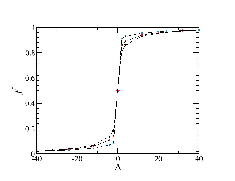
Figure 2: The fraction of cross-links in the steady state, $f^{\ast}$, as a function of $\Delta$. The simulation data (symbols) for $N=40,100,400$ are shown along with the theoretical predictions (denoted as $\tilde{f}$ in Section IV B (lines). In the large $N$ limit, $f^{\ast}\left(\Delta\right)$ approaches the Heaviside step function, $\Theta\left(\Delta\right)$.

Meanwhile, when $f$ is monitored in the ‘critical’ system ($\Delta_{c}=0$), it is found to execute an unbiased random walk bassler2015extreme between ‘soft walls’ at $f_{0}\sim 0.2$ and $1-f_{0}$. In other words, its stationary distribution, $P^{\ast}\left(f\right)$, resembles a mesa which spans nearly the entire allowed interval $\left[0,1\right]$. In subsequent simulation and theoretical studies bassler2015extreme ; bassler2015networks ; ZZEB2018 , we found that, as $N\rightarrow\infty$, the jump becomes maximal, while $f_{0}$ vanishes asymptotically as $\sqrt{\left(\ln N^{2}\right)/N}$. To emphasize, the latter means $P^{\ast}\left(f\right)\rightarrow 1$ for all $f\in\left[0,1\right]$, while $\sigma_{X}^{2}\rightarrow\mathcal{N}^{2}/12$! While such extreme features are the defining signatures of an ETE, this work is devoted to exploring the implications of such gargantuan fluctuations for the correlations between the links in our network.

III Correlations and fluctuations

The simplest measure of correlations in the 2D Ising model is the two-point function, $\left\langle s_{ij}s_{k\ell}\right\rangle-\left\langle s_{ij}\right\rangle\left\langle s_{k\ell}\right\rangle$, the integral (sum) of which is the variance $\left\langle M^{2}\right\rangle-\left\langle M\right\rangle^{2}$, a measure of the fluctuations. The analogs in $XIE$ are straightforward and, thanks to the permutation symmetry, they are relatively easy to compute (within the MFAs). In the analysis, we will be led naturally to the degree distributions of the nodes. Though, standard in the study of networks, their analogs in Ising model have rarely been examined. Beyond these, we will consider another natural measure of correlation for networks, the joint distribution of degrees of two nodes. Though easily measured in simulations, understanding their behavior remains a challenge.

III.1 Two point functions

We begin with the fluctuation-correlation identities, the foremost of which is simplest is

$$\sigma_{X}^{2}=\sum_{i,\eta,j,\gamma}\left\langle n_{i\eta}n_{j\gamma}\right\rangle-\left\langle X\right\rangle^{2}$$

Unlike the Ising case, ours is much simpler, since permutation symmetry of the steady state implies that there are only three distinct correlations. As $n_{i\eta}n_{i\eta}=n_{i\eta}$, we need to focus on cases where only one ($I$ or $E$) set of indices differ, or both $I$ and $E$ indices differ. Thus, we define the correlations, for any $i\neq j$ and $\eta\neq\gamma$,

$$\chi_{I} \equiv \left\langle n_{i\eta}n_{j\eta}\right\rangle-\left(f^{\ast}\right)^{2}$$

$$\chi_{E} \equiv \left\langle n_{i\eta}n_{i\gamma}\right\rangle-\left(f^{\ast}\right)^{2}$$

$$\chi_{IE} \equiv \left\langle n_{i\eta}n_{j\gamma}\right\rangle-\left(f^{\ast}\right)^{2}$$

since $\left\langle n_{i\eta}\right\rangle=\left\langle X\right\rangle/\mathcal{N}=f^{\ast}$. As a result, instead of the Ising relation, we find a much simpler fluctuation-correlation identity:

$$\frac{\sigma_{X}^{2}}{\mathcal{N}}=\chi_{0}+\left(N_{I}-1\right)\chi_{I}+\left(N_{E}-1\right)\chi_{E}+\left(N_{I}-1\right)\left(N_{E}-1\right)\chi_{IE}$$ (3)

where

$$\chi_{0}\equiv f^{\ast}\left(1-f^{\ast}\right)$$ (4)

is the variance of any single link: $\left\langle n_{i\eta}{}^{2}\right\rangle-\left\langle n_{i\eta}\right\rangle^{2}$. Of course, we can consider normalized correlations $\chi_{I,E,IE}/\chi_{0}$. But, as will be shown below, these present unnecessary theoretical challenges when we study the critical system.

There are three unknown $\chi$’s on the right of Eqn. (3). All can be determined in terms of fluctuations if we consider the degree distributions. In the stationary state, only two such distributions can be distinct: one associated with any $I$ and the other, with any $E$. To be precise, we write

$$\rho_{I}\left(k\right)\equiv\sum_{\mathbb{N}}\delta\left(k-\sum_{\eta}n_{i\eta}\right)\mathcal{P}^{\ast}\left(\mathbb{N}\right)$$

where $\delta$ is the Kronecker delta. Of course, we can write a similar expression for $\rho_{E}$. But, for symmetry reasons, it is better to consider the ‘hole-distribution’

$$\zeta_{E}\left(p\right)\equiv\sum_{\mathbb{N}}\delta\left(p-N_{I}+\sum_{i}n_{i\eta}\right)\mathcal{P}^{\ast}\left(\mathbb{N}\right)$$

From these, we study the averages and variances

$$\bar{k} \equiv \sum_{k}k\rho_{I}\left(k\right);~{}~{}\sigma_{k}^{2}\equiv\overline{k^{2}}-\bar{k}^{2}$$

$$\bar{p} \equiv \sum_{p}p\zeta_{E}\left(p\right);~{}~{}\sigma_{p}^{2}\equiv\overline{p^{2}}-\bar{p}^{2}$$

Focusing on the $I$’s for now, we find an expected result

$$\bar{k}=\sum_{\mathbb{N}}\left(\sum_{\eta}n_{i\eta}\right)\mathcal{P}^{\ast}\left(\mathbb{N}\right)=N_{E}f^{\ast}$$

which is also $\left\langle X\right\rangle/N_{I}$. Meanwhile,

$$\overline{k^{2}} = \sum_{k}k^{2}\rho_{I}\left(k\right)=\left\langle\sum_{\eta}n_{i\eta}\sum_{\gamma}n_{i\gamma}\right\rangle$$

$$= N_{E}\left[\left\langle n_{i\eta}\right\rangle+\left(N_{E}-1\right)\left\langle n_{i\eta}n_{i\gamma}\right\rangle\right]$$

so that $\sigma_{k}^{2}=N_{E}\left[f^{\ast}+\left(N_{E}-1\right)\left\langle n_{i\eta}n_{i\gamma}\right\rangle-N_{E}\left(f^{\ast}\right)^{2}\right]$, and we arrive at a ‘fluctuation-correlation identity for introverts’:

$$\frac{\sigma_{k}^{2}}{N_{E}}=\chi_{0}+\left(N_{E}-1\right)\chi_{E}$$ (5)

To be precise, we should state that there is an exact relationship between the variance of an $I$’s degree and the correlation of two of its links (to two different $E$’s). Since $\sigma_{p}^{2}$ is also the variance of the extroverts’ degree distribution, we easily find a similar identity for the extroverts:

$$\frac{\sigma_{p}^{2}}{N_{I}}=\chi_{0}+\left(N_{I}-1\right)\chi_{I}$$ (6)

Thus, all the $\chi$’s are known, once we obtain the variances: $\sigma_{k}^{2}$, $\sigma_{p}^{2}$, and $\sigma_{X}^{2}$. Note that, though we may consider similar quantities in the 2D Ising model, there is typically little reason to study the row- or column-magnetisation, i.e., the sums of the spins in a row or a column. Nevertheless, they do play crucial roles in highly anisotropic systems, such as driven diffusive systemsSZ95 ; DZ18 where the order parameter is the row (or column) magnetisation. A further note concerns $\sigma^{2}/N$ in Eqns.(3,5): For non-critical systems, we expect ‘normal’ fluctuations and these to be $O\left(1\right)$ in the thermodynamic limit, so that $\left(N_{I,E}-1\right)\chi_{I,E}$ and $\left(N_{I}-1\right)\left(N_{E}-1\right)\chi_{IE}$ should be good scaling variables.

There is another perspective of these identities which provides us with a gauge on how inter-dependent our variables are. In particular, if the degree of the $I$’s (and $E$’s) were iid’s from the same $\rho_{I}$ (and $\zeta_{E}$), then we would find

$$\sigma_{X}^{2}=N_{I}\sigma_{k}^{2}=N_{E}\sigma_{p}^{2}$$ (7)

However, Eqns. (5,6) can be exploited to recast Eqns (3) in several equivalent forms

$$\sigma_{X}^{2} = N_{I}\sigma_{k}^{2}+\mathcal{N}\left(N_{I}-1\right)\left[\chi_{I}+\left(N_{E}-1\right)\chi_{IE}\right]$$ (8)

$$= N_{E}\sigma_{p}^{2}+\mathcal{N}\left(N_{E}-1\right)\left[\chi_{E}+\left(N_{I}-1\right)\chi_{IE}\right]$$ (9)

Applied to Erdős-Rényi graphs E-R with average $f^{\ast}$, all these $\chi$’s vanish and Eqn. (7) is verified. In $XIE$, simulations show that these $\chi$’s are non-trivial and differences like $\sigma_{X}^{2}-N_{I}\sigma_{k}^{2}$ are significant.

We end this subsection with the analysis of the full stationary distribution of $X$

$$P^{\ast}\left(X\right)\equiv\sum_{\mathbb{N}}\delta\left(X-\sum_{i,\eta}n_{i\eta}\right)\mathcal{P}^{\ast}\left(\mathbb{N}\right)$$ (10)

and the related fixed $X$ ensembles, which are just cross-sections of $\mathcal{P}^{\ast}\left(\mathbb{N}\right)$ with a given $X$. They will play key roles in the analysis of the critical system. Their analogs in the Ising model, fixed $M$ ensembles, have received much attention for both physical and mathematical reasons. Many systems in nature with conserved $M$, e.g., liquid-vapor and binary alloys, are formulated in this manner and typically presented as the ‘Ising lattice gas’ YangLee52 . Such systems allow us to explore a variety of phenomena, e.g., phase co-existence, interfacial properties, nucleation, metastability and hysteresis. Mathematically, since fixed $M$ ensembles are conjugate to fluctuating $M$ ensembles with an external $H$, the associated free energies are Legendre transforms of each other (in the thermodynamic limit). Thus, they offer different approaches to analyze subtle singularities in the free energy, such as those associated with metastability. For the $XIE$ model, we discovered that fixed $X$ ensembles offer sufficient insight for constructing a mean-field approach that provides spectacular agreement with all simulation data, including those for the critical systemZZEB2018 . To avoid confusion, we will denote averages in such ensembles with extra caret above, e.g.,

$$\widehat{\left\langle\mathcal{O}\left(\mathbb{N}\right)\right\rangle}\equiv\sum_{\mathbb{N}}\mathcal{O}\left(\mathbb{N}\right)\delta\left(X-\sum_{i,\eta}n_{i\eta}\right)\mathcal{P}^{\ast}\left(\mathbb{N}\right)$$ (11)

with the understanding that $X$ (alternatively, $f\equiv X/\mathcal{N}$) is a control parameter here, with no fluctuations. Thus, for example,

$$\hat{\chi}_{0}=f\left(1-f\right)$$ (12)

is just a given constant, unlike $\chi_{0}$ in (4) which must be computed from $\left(N,\Delta\right)$. Clearly, for such ensembles, $\widehat{\sigma_{X}^{2}}\equiv 0$ and Eqn. (3) reduces to

$$0=\hat{\chi}_{0}+\left(N_{I}-1\right)\hat{\chi}_{I}+\left(N_{E}-1\right)\hat{\chi}_{E}+\left(N_{I}-1\right)\left(N_{E}-1\right)\hat{\chi}_{IE}$$ (13)

Thus, for fixed $X$ ensembles, some correlations must be negative. As will be shown below, these $\hat{\chi}$’s are crucial for understanding the extraordinary correlations in the critical system ($\Delta=0$).

In the next Section, we will present simulation data and MFA’s for understanding them.

III.2 Correlation in joint degree distributions

Beyond the two point function, there is a seemingly infinite variety of other possible measure of correlations. Here, we focus on one other quantity which appears natural for networks, namely, the joint degree distribution. In general, if $x$ and $y$ are independent variables distributed according to $\rho_{x}\left(x\right)$ and $\rho_{y}\left(y\right)$, then the joint distribution $\rho\left(x,y\right)$ is just the product $\rho_{x}\left(x\right)\rho_{y}\left(y\right)$. Thus, the difference between them is a good measure of the correlation between $x$ and $y$. In our case, we can study three such distributions: two $I$’s ($\rho\left(k,k^{\prime}\right)$), two $E$’s ($\zeta\left(p,p^{\prime}\right)$), and one of each ($\mu\left(k,p\right)$). To save notation, we will use, as above, $k$ for the degree associated with an $I$ and $p$ for the ‘hole-degree’ associated with an $E$. Thus, e.g.,

$$\mu\left(k,p\right)=\sum_{\mathbb{N}}\delta\left(k-\sum_{\eta}n_{1\eta}\right)\delta\left(p-N_{I}+\sum_{i}n_{i1}\right)\mathcal{P}^{\ast}\left(\mathbb{N}\right)$$ (14)

is the joint distribution for an $I$ and an $E$. In the steady state, all nodes in each group should be equivalent and so, we write $1$’s in the above for convenience. The differences, such as

$$\mu\left(k,p\right)-\rho\left(k\right)\zeta\left(p\right)$$ (15)

are measures of the correlations between the two nodes. Finding a viable theory to provide quantitative insights into these quantities has been elusive. Below, we will only show simulation data and make some qualitative statements. In this context, we will present the ‘normalized’ differences, e.g.,

$$C_{IE}\left(k,p\right)\equiv\frac{\mu\left(k,p\right)}{\rho\left(k\right)\zeta\left(p\right)}-1$$ (16)

Before proceeding to the data, we should emphasize that, though $\rho\left(k,k^{\prime}\right)$ and $\rho\left(p,p^{\prime}\right)$ reduce to the respective products for random $\mathbb{N}$’s (i.e., Erdős-Rényi bipartite graphs), this is not the case for the mixed distribution $\mu$. The reason is that, for any $I$-$E$ pair, their degrees are not entirely independent, as both $k$ and $p$ are affected (oppositely) by the one link between them. In particular, $n_{11}$ appears in both $\delta$ functions in Eqn. (14), so that the sum does not factorize into the product of sums over $\mathcal{P}^{\ast}$, even if $\mathcal{P}^{\ast}$ itself factorizes. Deferring details of this analysis to an Appendix, we only quote the result here

$$C_{IE}^{ER}\left(k,p\right)=\left(\frac{k}{\bar{k}}-1\right)\left(1-\frac{p}{\bar{p}}\right)$$ (17)

where $\bar{k}/N_{E}=1-\bar{p}/N_{I}$ is the probability of any element in $\mathbb{N}$ being unity and illustrated in Fig 11. Being a simple quadrupole in the $k$-$p$ plane, this scaling form clearly displays the anti-correlation between the particle- and the hole-count (i.e., one more $1$ in a row being correlated with one less $0$ in a column).

IV Simulation results and mean field approaches

This Section is devoted to simulation studies and our understanding through mean field approximations. For the two point correlations and fluctuations (variances in the degrees of a node or the total number of cross-links), we considered systems with $N=40,100$, and $400$, performing 10 independent runs of $10^{7}\times\mathcal{N}$ MCS for each data point, where $\mathcal{N}=N_{I}\times N_{E}$. To obtain the averages in the steady state, $\left\langle...\right\rangle$, we discard the first $10^{5}\times\mathcal{N}$ MCS and take measurement every $\mathcal{N}$ MCS. Following earlier studies of our model liu2013extraordinary ; bassler2015extreme , we first use $\Delta$ as a control parameter, in the range $\left[-40,40\right]$. Thanks to $I$-$E$ symmetry, the degrees of an $I$, $\rho_{I}\left(k\right)$, in the stationary state is the same as the distribution of holes, $\zeta_{E}\left(p\right)$, for an $E$ at the opposite $\Delta$. Though not display here, we have explicitly verified that such symmetries hold. Thus, in the following, we will consider on only $\rho\left(k\right)$, where we also dropped the subscript for simplicity. This symmetry also implies that the stationary distribution of cross-links, $P^{\ast}\left(X\right)$, obeys

$$P^{\ast}\left(X;N,\Delta\right)=P^{\ast}\left(\mathcal{N}-X;N,-\Delta\right)$$

so that we can focus only on results for, say, $\Delta\leq 0$. Now, as Fig. 2 shows, as we study larger and larger systems with $\Delta\neq 0$, we have access to a more and more limited region of $f$. On the other hand, from Ref. ZZEB2018 , we see that a critical system behaves like a superposition of fixed $f$ ones – from $f_{0}$ to $1-f_{0}$. Thus, we can access the intermediate $f$ regime by using fixed $f$ (or $X$) ensembles. To generate such ensembles by Monte Carlo simulations, we begin with a random $\mathbb{N}$ consisting of precisely $X$ ‘particles’ and carry out the standard Kawasaki particle-hole pair exchanges according to Metropolis rates (i.e., accepting the attempt with probability $\min\left\{1,e^{-\mathcal{H}}\right\}$ where $\delta\mathcal{H}$ is the difference in $\mathcal{H}$ as a result of the exchange). To obtain $\widehat{\left\langle...\right\rangle}$, we discard the first $10^{5}\times\mathcal{N}$ MCS and take measurement every $\mathcal{N}$ MCS over $10$ independent runs.

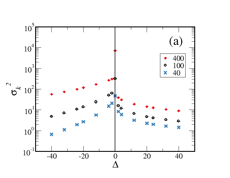
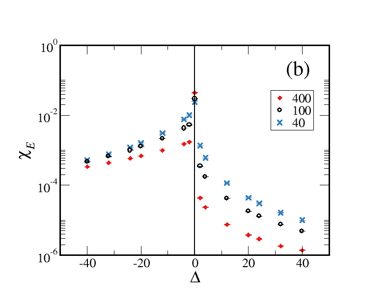
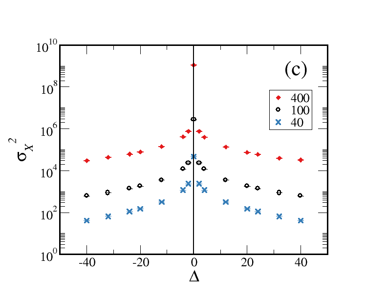
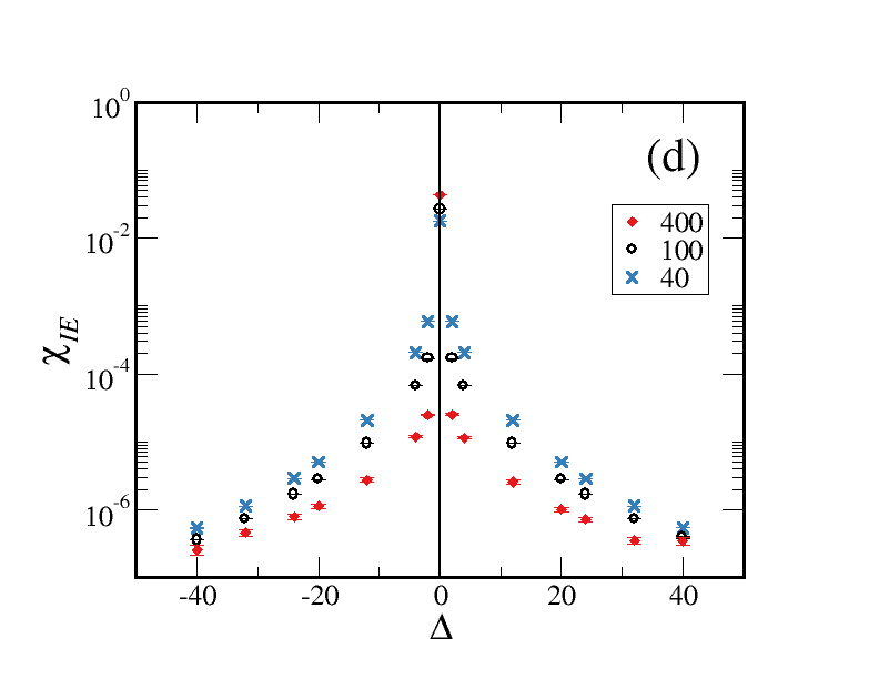
Figure 3: Simulation data for variances and correlations plotted against $\Delta$. The variances shown are for (a) the introvert degree distribution, $\sigma^{2}_{k}$, and (c) the total number of cross-links, $\sigma^{2}_{X}$. The correlations shown are for two links with only the E’s being distinct, $\chi_{E}$, (b) and (d) both the I’s and E’s being different, $\chi_{IE}$.

Although the data in Fig. 3 seem peculiar at first glance, we are able to understand all the unusual properties in two steps. First, we derived identities which relate all distinct two-point correlations and the various variances, so that we need to focus our theoretical considerations on only, say, the $\sigma^{2}$’s. For the degree distributions, we exploit a version of the self-consistent mean field approach (SCMF), first introduced in Ref. bassler2015extreme , which has been improved in several aspects. From its predictions for $\rho\left(k\right)$, we arrive at a good understanding of the fluctuations $\sigma_{k}^{2}$. The second step follows the track in Ref. ZZEB2018 , which leads us to an excellent approximation for $P^{\ast}\left(X\right)$ and therefore, predictions for $\sigma_{X}^{2}$, the fluctuations in $X$.

Ending this Section, we will present data for the joint degree distributions (e.g., $\mu\left(k,p\right)$) and the implied correlations (e.g., $C_{IE}\left(k,p\right)$). Unfortunately, finding a viable approximation for these proves elusive. We provide a hint at the level of complexity involved in understanding such joint distributions, by computing the non-trivial $C_{IE}\left(k,p\right)$ for random bipartite graphs exactly.

IV.1 Fluctuations and correlations for non-critical systems ($\Delta\neq 0$ and fixed $X$ ensembles)

We begin with Fig. 3, which shows two sets of fluctuations and correlations.

A casual glance of this figure does not hint at any easily tractable behavior. Indeed the data appear in general to be quite peculiar, displaying up to three regimes, i.e., $\Delta$ being negative, positive, and zero. To understand these unusual properties and to develop a more coherent picture, we first note that, though there are apparent differences between the fluctuation data and the correlations, they are indeed related by the identities derived above. Since these are exact relations, there is no need for us to understand the behavior of both. To be specific, we will focus on only the fluctuations, as we had mean field theories for the associated distributions. We should emphasize that our data are in complete agreement with Eqns. (3,5,6), giving us confidence that a steady state has been established.

Next, since $\rho$ involves $N_{E}$ binary random variables, we expect the variance $\sigma_{k}^{2}$ to scale with $N_{E}$. Thus, instead of the raw data, we plot the ‘normalized’ version: $\sigma_{k}^{2}/N_{E}$in Fig. 4a.

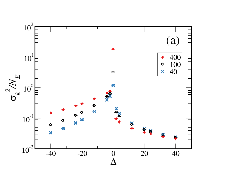
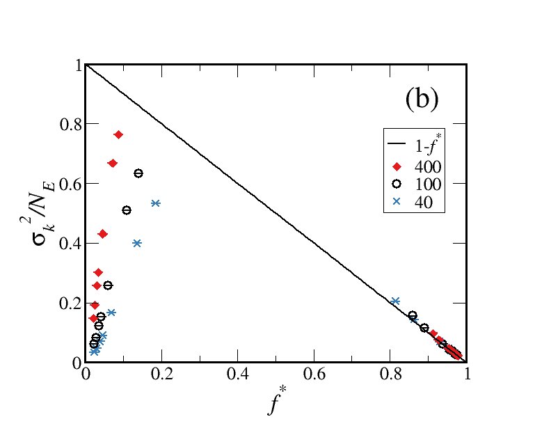
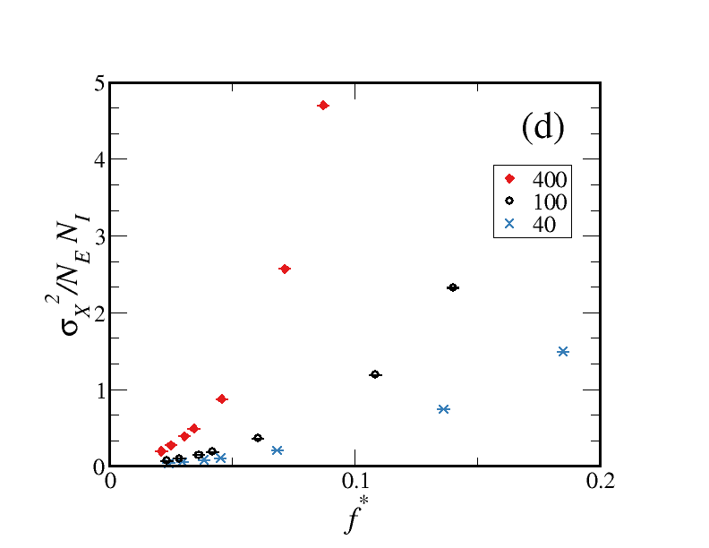
Figure 4: (a,c) Simulation data from 3a,c ‘normalized’ by $N_{E}$ and $\mathcal{N}$ respectively. (b) Same data set as in (a), except the critical system, plotted against $f^{\ast}$ instead of $\Delta$. (d) Same data set as in (b) plotted against $f^{\ast}$; since $\sigma_{X}^{2}$ is symmetric about $\Delta=0$, only the small $f^{\ast}$ ($\Delta<0$) region is displayed.

Similarly, we show $\sigma_{X}^{2}/\mathcal{N}$ in panel (b). No obvious systematics emerge in this replot. Now, we note that, for various $N$’s, $f^{\ast}\left(\Delta\right)$ is a rather complicated and singular function (See Fig. 2.). That provides a motivation for us to plot the variances against $f^{\ast}$: Fig. 4b,d. Only a minor improvement is seen: tolerable data collapse for $\sigma_{k}^{2}/N_{E}$ in the $f^{\ast}>1/2$ ($\Delta>0$) regime. Meanwhile, if we wish to study larger systems, the accessible region of $f^{\ast}$ (with $\Delta\neq 0$) becomes more severely limited. In an effort to explore the ‘inaccessible’ region, we extended our studies to fixed $X$ ensembles of the critical ($N_{E}=N_{I}$) system. Of course, for such systems, $\widehat{\sigma_{X}^{2}}\equiv 0$ and we are left with only $\widehat{\sigma_{k}^{2}}$, the data for which are shown in Fig. 5a.

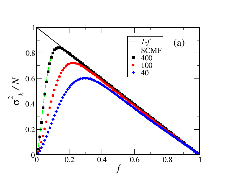
(a)

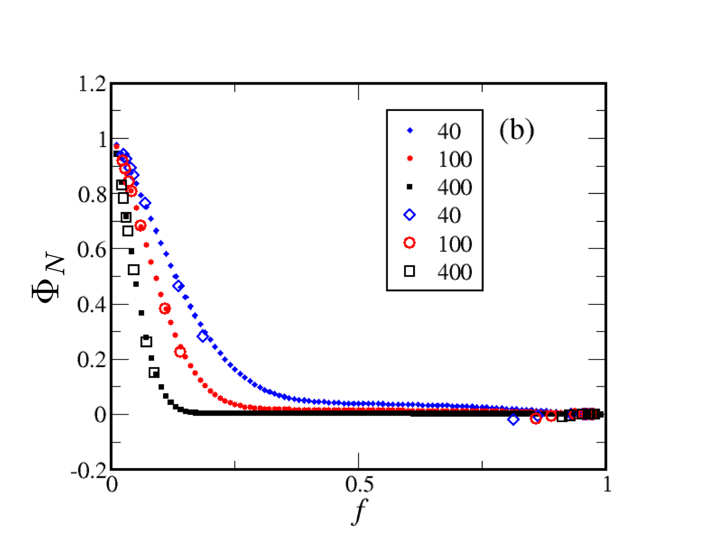
(b)

Figure 5: (a) Simulation data for $\widehat{\sigma_{k}^{2}}/N$ (solid symbols) using fixed $X$ (i.e., $f$) ensembles for $N=40,100,$ and $400$. As $N$ increases, the data is seen to converge on $1-f$ (solid line). The dashed line (green online) is the prediction from our SCMF theory. (b) The difference $\Phi_{N}$ (18), highlighting the non-uniform convergence, as $N\rightarrow\infty$, to a singular step function: $1-\Theta\left(f\right)$. In addition, $\Phi_{N}$’s from the data in from Fig. 4b (open symbols) are displayed for comparison. See text for discussions.

Note that these points are displayed alongside the data from Fig. 4b, showing that the new points indeed “fill in the gap.” Though the two sets of data are mostly the same, there are small differences, the origins of which remain to be explored further. We conjecture at least two possible sources: (i) Since $f$ is not fixed in the $\Delta\neq 0$ systems (the data point being plotted at $f^{\ast}$ here), those fluctuations can contribute to the systematically larger $\sigma_{k}^{2}/N_{E}$, especially discernible at the $f\sim 1$ regime. (ii) Finite size effects are unlikely to be the same for the two sets of systems, leading to differences seen in the figure. Finally, we should mention that there are clear “shoulders,” especially visible in the $N=40$ data, which are manifestations of the underlying mesa-like $P^{\ast}\left(X\right)$. A detailed understanding of such behavior is beyond the scope of this study and, though quite feasible, will be published elsewhere.

Turning from these small differences to the more prominent common features, the most obvious feature is the non-uniform convergence of $\widehat{\sigma_{k}^{2}}/N$ to the simple function $\left(1-f\right)$ as $N$ increases. One may try to collapse the rise for small $f$ by a naive function like $Nf$. However, the quality of such collapse is poor and we cannot find any theoretical justification for such a form. As will be shown in the next subsection, there exists a non-trivial scaling function for the difference:

$$\Phi_{N}\equiv\left(1-f\right)-\widehat{\sigma_{k}^{2}}/N$$ (18)

Shown in Fig. 5b, $\Phi_{N}$ displays the same non-uniform convergence properties, but to the singular step function $\Phi_{\infty}\left(0\right)=1;\Phi_{\infty}\left(f>0\right)=0$.

Finally, let us return to the fluctuations in $X$ and mention a curious phenomenon: Dividing $\sigma_{X}^{2}/\mathcal{N}$ by a further factor of $N_{I}$, we find reasonable data collapse onto $f^{2}$! There seems to be no theoretical basis for this behavior and perhaps its appearance is simply ‘an accident.’ Instead, as the detailed analysis in the next subsection will show, there is a sound basis for collapse onto a different function, namely, $-1-1/f^{\ast}\Delta$.

IV.2 Mean field approaches (MFA) and theoretical understanding

Though the stationary distribution ($\mathcal{P}^{\ast}$) for our model is explicitly known, it is quite challenging to obtain exact theoretical results, especially since the system displays an ETE. Surprising progress had been made, however, through a series of mean field approximations. Though not systematic, MFAs are based on sound intuitions and captured much of the essence of the extraordinary properties in our model. Referring the reader to Refs. liu2013extraordinary ; bassler2015extreme ; ZZEB2018 for the justifications and derivations, we provide only a brief summary here. The basis of our MFA is the finite Poisson distribution (FPD):

$$Q\left(n;x,N\right)=\frac{x^{n}}{e_{N}\left(x\right)n!};~{}~{}n=0,1,...,N$$

where $e_{N}\left(x\right)\equiv\sum_{0}^{N}x^{n}/n!$. Since it is rarely discussed in the literature, we collected in an Appendix a list of its properties, the most useful of which are $\bar{n}=x\left(1-Q\left(N\right)\right)$ and $\overline{n\left(n-1\right)}=x^{2}\left(1-Q\left(N\right)-Q\left(N-1\right)\right)$. The FPD enters when we study the introvert degree distribution in the steady state

$$\rho\left(k\right)=Q\left(N_{E}-k;\lambda,N_{E}\right)$$ (19)

as we balance the rate of losing of a link to that for gaining one. In considering the gain rate, the number of $E$’s not already connected to our $I$ is $N_{E}-k$, while the probability of an $E$ making a link to our $I$ is a stochastic variable. The parameter $\lambda$ is meant to capture (the inverse of) the latter probability and so, was argued previously ZZEB2018 (where fixed $f$ ensembles were used) to be $N_{I}\left(1-f\right)$. However, when $\bar{k}$ is computed with this $\rho$ (and $\lambda$), we find

$$\bar{k}=N_{E}-\lambda\upsilon$$ (20)

where $\upsilon$ is the following function of $\lambda$

$$\upsilon\equiv e_{N_{E}-1}\left(\lambda\right)/e_{N_{E}}\left(\lambda\right)=1-\rho\left(0\right)$$ (21)

and represents the fraction of ‘unsatisfied’ $I$’s (those with one or more links). In other words, given $\lambda$, the FPD will lead to the above $\bar{k}$ and therefore a fraction of cross-links being $\bar{k}/N_{E}=1-\lambda\upsilon$. But if we set $\lambda$ to $N_{I}\left(1-f\right)$, then this $1-\lambda\upsilon$ can be $f$ only if $\lambda$ takes on a specific value, $\tilde{\lambda}$, which satisfies

$$\tilde{\upsilon}=N_{E}/N_{I}$$ (22)

where $\tilde{\upsilon}\equiv\upsilon\left(\tilde{\lambda}\right)$. To emphasize this issue, if we insist on imposing three control parameters ($N_{E}$, $N_{I}$, and $f$ – in fixed $X$ ensembles), then the FPD in Ref. ZZEB2018 cannot be a self-consistent approximation in general. Remarkably, if we do not restrict the value of $f$, then it will settle, on average, at a $f^{\ast}$ that corresponds to Eqn. (22). We will return to this question when we study $P^{\ast}\left(X\right)$ below.

Here, let us modify the MFA in Ref. ZZEB2018 to be a self-consistent mean field theory (SCMF), i.e., we will choose $\lambda$ to be the solution to

$$\lambda\upsilon\left(\lambda\right)=N_{E}\left(1-f\right)$$ (23)

so that the Ansatz (19) will agree with $\bar{k}=N_{E}f$ in all cases. Note that, in the context of the FPD, this relation provides a 1-1 mapping between $f$ and $\lambda$. In our case, it is straightforward to verify that $df/d\lambda$ is strictly negative.

Once we grasp the $\lambda$-$f$ connection, we can proceed to compute $\widehat{\sigma_{k}^{2}}$ as a function of $f$. In particular, we seek the non-trivial cross-over behavior for large $N$. As noted above, the difference $\Phi_{N}$ is more convenient for displaying these properties of $\widehat{\sigma_{k}^{2}}$. After some algebra, we find a compact expression:

$$\Phi_{N}=\lambda\xi f$$ (24)

where

$$\xi\equiv 1-\upsilon$$ (25)

is the fraction of ‘satisfied’ $I$’s (those no links). The simple form for $\Phi_{N}$ is deceptive, however, as both $\lambda$ and $\xi$ are complicated functions of $f$. The details of the analysis are quite involved and so, deferred to an Appendix. Here, let us only present the result. As displayed in Fig.5, $\Phi_{N}$ drops steeply from $1$ down to near $0$ at cross-over values which diminishes as $N$ increases. Nevertheless, as shown in Fig 6a, we find good quality data collapse (especially within $\left(-1,+2\right)$, even for systems as small as $40$) when this difference is plotted against a scaling variable

$$w=\frac{N+1-\lambda}{\sqrt{2\left(N+1\right)}}$$

which emerges naturally from the analysis of our SCMF theory. As $N\rightarrow\infty$, $\Phi_{N}$ is well approximated by the analytic scaling function

$$\Phi_{N}\simeq 2\mathcal{E}\left(\mathcal{E}+w\right)$$ (26)

where

$$\mathcal{E}\left(w\right)\equiv 1\left/\sqrt{\pi}e^{w^{2}}\left[1+\mathop{\rm erf}\left(w\right)\right]\right.$$

Both the numerical evaluation of $\Phi_{400}$ and this analytic asymptotic form are shown in the figure for comparison.

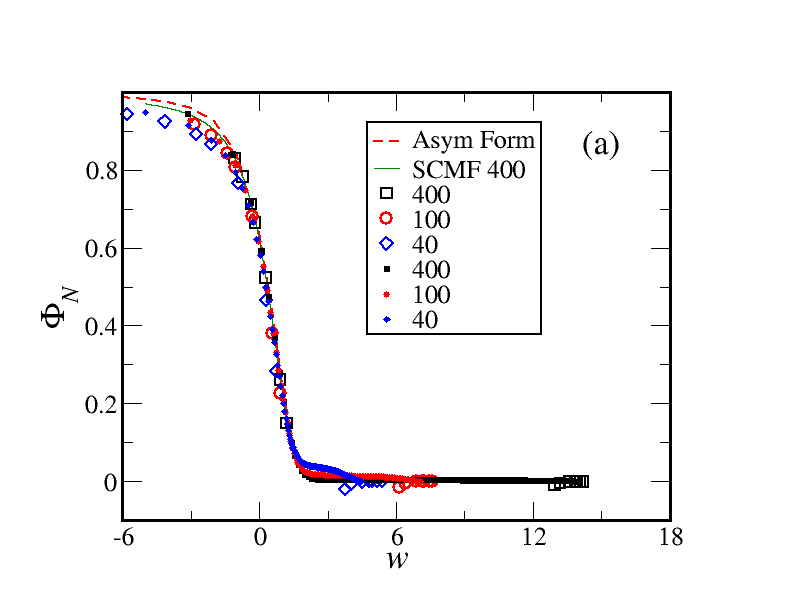
(a)

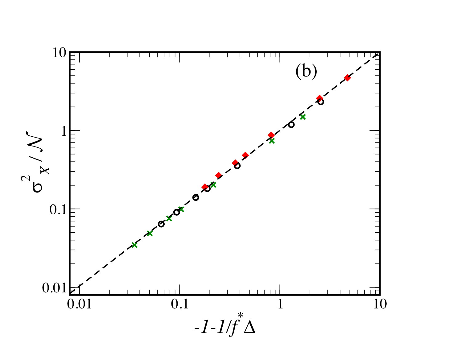
(b)

Figure 6: (a) $\Phi_{N}$ from Fig.5b (same symbols used) plotted against the scaling variable $w$, showing good quality data collapse (especially within $\left(-1,+2\right)$, even for our small systems). In addition to the data points, we display two curves from SCMF theory (dash red line for the analytic, asymptotic form (26) and sold black line from numerical evaluation with $N=400$) (b) Log-log plot of $\sigma_{X}^{2}/\mathcal{N}$ – the data set in Fig.4d – against the scaling variable $-1-1/f^{\ast}\Delta$. Finite size effects, especially for the $N=40$ case, restrict the scaling region to a small ragne of $w$, in which good quality data collapse is seen over an order of magnitude (two orders for the $N=400$ data). Dashed line is from numerical evaluation of the SCMF theory, Eqn. (28). Solid line is the asymptotic analytic form, Eqn. (26).

To end this subsection, we turn to the fluctuations in $X$ in non-critical systems, $\sigma_{X}^{2}/\mathcal{N}$. As shown in Ref. ZZEB2018 , by considering the balance of gain and loss of a link in a single attempt, the equation for the steady state $P^{\ast}\left(X\right)$ is

$$N_{E}\left(1-\zeta_{E}\left(0\right)\right)P^{\ast}\left(X-1\right)=N_{I}\left(1-\rho_{I}\left(0\right)\right)P^{\ast}\left(X\right)$$

Again, thanks to $I$-$E$ symmetry, we can focusing on the regime of small $X$ (or $N_{E}/N_{I}<1$), say. Then, we can approximate this equation by

$$\left(N_{E}/N_{I}\right)P^{\ast}\left(X-1\right)\cong\upsilon P^{\ast}\left(X\right)$$ (27)

It is clear that, since $\upsilon$ is a monotonic function of $f$ or $X$, the above recursion relation for $P^{\ast}$ will lead to a maximum occurring at $\tilde{f}$ (i.e., $\tilde{X}=\tilde{f}\mathcal{N}$) which satisfies the equation $\tilde{\upsilon}=N_{E}/N_{I}$. To emphasize this point, the system will be most likely found at $\tilde{f}$ and so, we will identify it with $f^{\ast}$, the average value of $f$ when the system settles in the steady state. Note that the condition (27) corresponds to setting the first derivative of $\ln P^{\ast}$ to zero. Beyond that, both theory and data support the expectation that, as $N\rightarrow\infty$, $P^{\ast}\left(X\right)$ approaches a Gaussian around $\tilde{X}$. Thus, the curvature of $\ln P^{\ast}$ there should provide us with a good approximation (denoted by $\cong$) for the fluctuations in $X$. Specifically, we expect

$$-1/\sigma_{X}^{2} \cong \ln P^{\ast}\left(\tilde{X}+1\right)-2\ln P^{\ast}\left(\tilde{X}\right)+\ln P^{\ast}\left(\tilde{X}-1\right)$$

$$\cong \ln P^{\ast}\left(\tilde{X}+1\right)-\ln P^{\ast}\left(\tilde{X}\right)$$

In other words, $-1/\sigma_{X}^{2}$ is related to $\left.\partial_{X}\ln\upsilon\right|_{\tilde{X}}$. After some algebra, we arrive at a concise expression

$$\sigma_{X}^{2}/\mathcal{N}\simeq\frac{1}{-\tilde{f}\Delta}-1$$ (28)

with corrections of $O\left(N^{-1/2}\right)$ expected. We emphasize that $\Delta<0$ for the regime of interest here, so that the first term is positive. Though we can compute $\tilde{f}$ in terms of the control parameters $\left(N,\Delta\right)$, we cannot provide a simple expression as it depends on implicit relations like $\tilde{\upsilon}=N_{E}/N_{I}$. Nevertheless, we can expect that as $N$ increases with $|\Delta|=O\left(1\right)$, $\tilde{f}$ decreases significantly (with upper bound $\sqrt{\ln N^{2}/N}$) and so, $\sigma_{X}^{2}/\mathcal{N}$ should become anomalously large. Such a behavior is hardly surprising, as this limit corresponds to approaching the transition point of our ETE. More importantly, when all the simulations results are plotted against the scaling variable, we find high quality data collapse (Fig. 6b), even though our $N$’s are not so large. It is reasonable to conclude that the SCMF here is very successful in capturing the essence of the anomalous fluctuations in the $XIE$ model.

IV.3 Fluctuations and correlations for critical systems

Finally, we turn to the behavior of critical systems ($\Delta=0$). Here also, the fluctuation-correlation identities were verified to hold and so, we again focus our attention only on the former. As Figs 3 and 4 shows, the fluctuations of the are considerably larger than the ones in the non-critical systems or the fixed $X$ ensembles. We devote this subsection to a brief summary of how this extraordinary phenomenon can be understood. We follow the approach in Ref. ZZEB2018 , i.e., to regard the critical system as a superposition of fixed $X$ ensembles, weighted by the critical $P^{\ast}\left(X;N,0\right)$. Then, for any observable, we have

$$\left\langle\mathcal{O}\right\rangle=\sum_{X}\widehat{\left\langle\mathcal{O}\right\rangle_{X}}~{}P^{\ast}\left(X;N,0\right)$$

For example, this approach predicted $\rho\left(k\right)$ and $\zeta\left(p\right)$ successfullyZZEB2018 . Applying it to the fluctuations of the degree, $\sigma_{k}^{2}$, is straightforward, as we simply construct the convolution of $\widehat{\sigma_{k}^{2}}$ with $P^{\ast}\left(X\right)$. The former is given above, while the latter can be found in Ref. ZZEB2018 . Skipping the details, the results for the three $N$’s are in excellent agreement with data. Of course, this approach allows us to understand why these fluctuations are so much larger than the non-critical ones. While $P^{\ast}\left(X;N,\Delta\neq 0\right)$ are Gaussian-like with a relatively normal spread in $X$, $P^{\ast}\left(X;N,\Delta=0\right)$ resembles a mesa, with sharp drop-offs which approach the boundariesZZEB2018 as $N\rightarrow\infty$. Indeed, in that limit, there is no need to compute the location of these drop-offs as $P^{\ast}\left(X\right)$ becomes a uniform distribution in $\left[0,\mathcal{N}\right]$. Then, $\left\langle X^{2}\right\rangle=\mathcal{N}^{2}/3$ and $\sigma_{X}^{2}=\mathcal{N}^{2}/12$. In other words, the divergence of Eqn. (28) at $\Delta=0$ is bounded by $\mathcal{N}/12$ for large, but finite, $\mathcal{N}$. Our data for $\mathcal{N}=40^{2},100^{2},400^{2}$ are plotted in Fig. 7, along with a line showing $\mathcal{N}^{2}/12$.

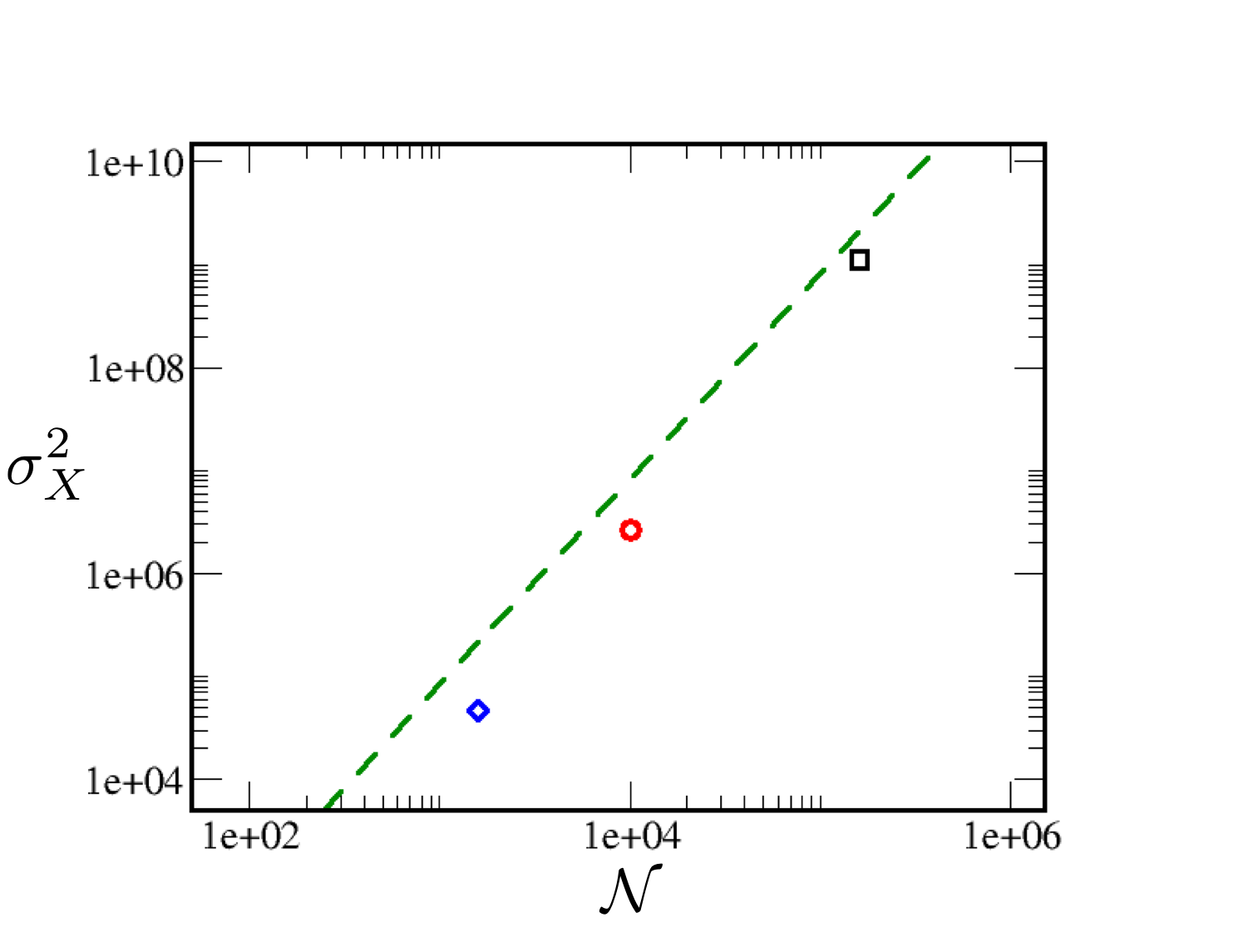
Figure 7: Data for $\sigma_{X}^{2}$ (Y axis) in the three critical systems (symbols) in Fig.3c vs. $\mathcal{N}$ (X axis), along with the (dashed) line $\mathcal{N}^{2}/12$.

This figure clearly shows that $\sigma_{X}^{2}\propto\mathcal{N}$ is not satisfied, as it approaches the upper bound for the larger $\mathcal{N}$’s. To close this subsection, let us point to the analog in the 2D Ising model, where the fluctuations of the total magnetisation (which corresponds to our $X$) of a finite $L\times L$ system diverge anomalously at the critical point: $\sigma_{M}^{2}\sim L^{4-2\beta/\nu}=\mathcal{N}^{15/8}$.

IV.4 Joint degree distributions

Lastly, we present results of the first explorations into joint distributions of degrees. For simplicity, we only provide data for $\rho\left(k,k^{\prime}\right)$ (distribution of degrees of two $I$’s) and $\mu\left(k,p\right)$ (degrees of an $I$ and a $E$) in systems with $N=100$. To highlight the presence of correlations, we mostly present the difference between these and the products of the single node degree distributions, normalized by the latter, i.e.,

$$C_{II}\left(k,k^{\prime}\right)\equiv\frac{\rho\left(k,k^{\prime}\right)}{\rho\left(k\right)\rho\left(k^{\prime}\right)}-1;~{}~{}C_{IE}\left(k,p\right)\equiv\frac{\mu\left(k,p\right)}{\rho\left(k\right)\zeta\left(p\right)}-1$$ (29)

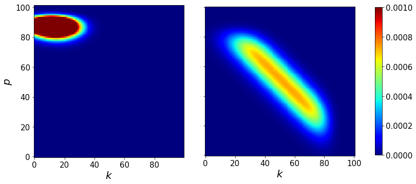
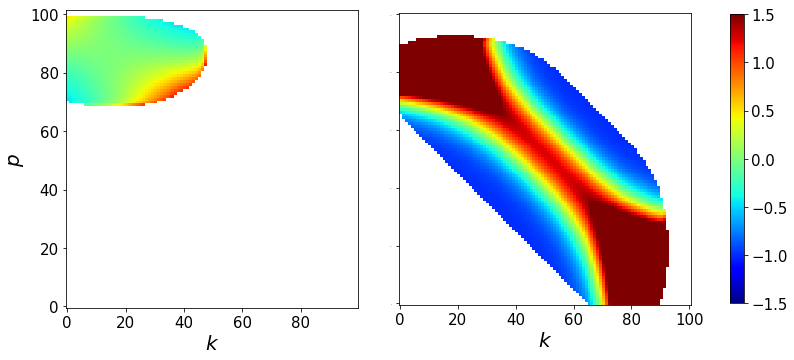
Figure 8: Upper panels: The joint degree distribution $\mu\left(k,p\right)$ for two $N=100$ systems, near criticality (left, $\Delta=-2$) and at criticality (right, $\Delta=0$). The elongated region in the latter is a reflection of the mesa-like distribution, $P^{\ast}\left(X\right)$, at criticality. Lower panels: The correlations, Eqn. (29), associated with the upper panels. Note the (highly distorted) quadrapolar form, i.e., correlated near $k=-p$ and anticorrelated close to $k=p$.

As above, we first consider $XIE$ systems with fixed $\Delta$. To help the reader visualize the joint distribution itself, we present $\mu\left(k,p\right)$ for $\Delta=-2$ and $\Delta=0$ in the upper panels of Fig. 8. As expected from our studies of the single node distributions $\rho$ and $\zeta$, $\mu$ is mostly narrowly distributed around $\left(k,p\right)\cong\left(14,86\right)$ in the former, but spread over a wide range of values along the line $k+p\cong 50$ in the latter. These qualitative features are shared by the product $\rho\left(k\right)\zeta\left(p\right)$ of course. The correlations $C_{IE}\left(k,p\right)$ are displayed in the lower panels of Fig. 8 and hints at a quadrupolar form: positive along the $k=-p$ diagonal and negative along the $k=p$ line. Though the qualitative aspects of this phenomenon are easily understood (as they also occur for the Erdős-Rényi random ensemble, Fig. 11d), the quantitative features are more subtle and yet to be examined in detail. Undoubtedly related to the two-point correlations $\chi$, they remaned to be well understood. Turning to fixed $X$ ensembles, a more unexpected feature is revealed - octapolar $C_{IE}\left(k,p\right)$, as illustrated in Fig. 9a for a $f=0.5$ system. It is unclear what is the origin of such behavior, though very small traces of it are visible in the corresponding fixed $X$ Erdős-Rényi ensemble: Fig. 9.

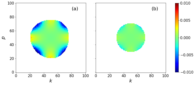
Figure 9: Comparison of $C_{IE}\left(k,p\right)$ in two fixed $f=0.5$ ensembles: $XIE$ (a) and Erdős-Rényi (b). Note the octaploar patterns in both.

The next set of figures (10) provide a similar challenge, as they show quadrupolar patterns associated with the joint distribution of two introverts, $C_{II}\left(k,k^{\prime}\right)$, in fixed $X$ ensembles of the $XIE$ model. Note that, unlike $C_{IE}$, both variables correspond to degrees (not ‘holes’). As a result, the $f=0.2$ distribution are centered around $k=k^{\prime}=20$. We conjecture that the positive/negative correlations along the two diagonals are manifestations of the fixed $X$ constraint, as increases in $k$ must be compensated by decreases in $k^{\prime}$. Perhaps there is a deeper connection to the octapolar pattern in $C_{IE}\left(k,p\right)$. Quantitative analyses are underway but progress will be challenging, as techniques similar to those used to build a SCMF for $\rho$ and $\zeta$ fail for joint distributions.

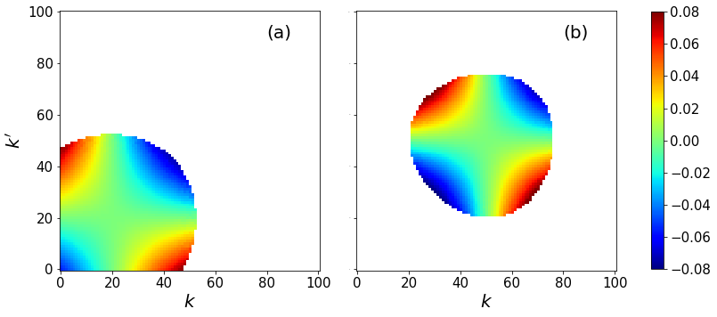
Figure 10: Correlations between two introverts, $C_{II}\left(k,k^{\prime}\right)$, in two fixed $X$ ensembles of $XIE$: (a) $f=0.2$ and (b) $f=0.5$.

To end this section, we will consider the simpler case of Erdős-Rényi bipartite graphs, i.e., randomly distributed cross-links, as the associated distributions are amenable to analytic tools and can display non-trivial patterns. First, we study ensembles in which links are present with a fixed probability, $r$. Clearly, we expect $C_{II}^{ER}\left(k,k^{\prime}\right)$ to vanish, since there is no correlation between two the entries on different row of $\mathbb{N}$. This property is illustrated in Fig. 11a,b for $r=0.2$ and $0.5$. By contrast, as shown in Appendix A, we expect $C_{IE}^{ER}\left(k,p\right)$ to be non-trivial, as seen in Fig. 11c,d. We verified that the data are in reasonably good agreement (i.e., within statistical errors) with the exact quadrupolar form of Eqn. (17). Another class of ER bipartite network is the fixed $f$ ensemble of random graphs, i.e., all $\mathbb{N}$’s with a fixed fraction ($f$) of links, each with equal weight. Although we expect the two ensembles to be equivalent in the $\mathcal{N}\rightarrow\infty$ limit, there appear to be significant differences, as illustrated in Fig. 9b for $C_{IE}^{ER}\left(k,p|X\right)$ in a system with $X=\left(100\right)^{2}/2$. Not only is the magnitude much smaller than the unconstrained $C_{IE}^{ER}\left(k,p\right)$ with $r=0.5$, there is a hint of a octapole instead of a quadrupole. This puzzling aspect remains to be understood fully. While further analysis is feasible, it is beyond the scope of this paper. What we wish to emphasize here is that, even in the case of ‘simple ER’ bipartite graphs, we find a non-trivial pattern, similar to the one we found in the constrained $XIE$ model. Clearly, joint distributions offer new and interesting horizons for future studies.

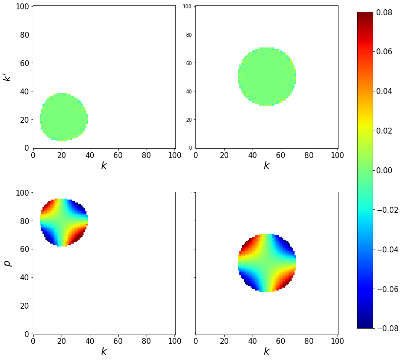
Figure 11: Correlations in Erdős-Rényi bipartite ensembles with links being present with probability $r$. Upper panels: $C_{II}^{ER}\left(k,k^{\prime}\right)$ between two introverts. Lower panels: $C_{IE}^{ER}\left(k,p\right)$, between an $I$ and an $E$. On the left are ensembles with $r=0.2$ and on the right, $r=0.5$.

V Summary and Outlook

In this study, we examined the correlations and fluctuations in the $XIE$ model. Given that it can be formulated as an 2D Ising model with a complicated Hamiltonian (which exhibits multi-spin and long-ranged interactions: Eqn (1)) and that it displayed an extreme Thouless effect, we should expect serious correlations and fluctuations. Focusing on two-point correlations, we showed that, in the steady state, the permutation symmetry of the model implies that there are only three independent correlations. In $XIE$, these correspond to two links which share one $I$ but connected to two $E$’s ($\chi_{E}$), one $E$ and two $I$’s ($\chi_{I}$), or having no common nodes ($\chi_{IE}$). In the Ising language, these would be two spins on the same row, in the same column, in different rows and columns. Since there are just three quantities, they can be uniquely related to three fluctuations: the degrees of $I$ and $E$ and the total number of cross-links. In the Ising language, these would be the total magnetisation in a row, a column, and the entire system. We have verified these fluctuation-correlation identities and chose to focus on the fluctuations only.

In general, there are two types of fluctuations, associated with non-critical and critical systems. Drawing an analogy with the 2D Ising model, we note not only some similarities between the two point correlations and fluctuations of certain quantities, but also the unusual aspects found in our system. In all cases, a self-consistent mean-field theory, improved from previous mean-field approaches, appears to capture the essence of the Monte Carlo data we obtained. Thus, we conclude that the properties of these quantities are well understood. An important lesson is that, under the right circumstances, mean field approaches can be adequate in describing large fluctuations and strong correlations. Finally, we presented preliminary studies of joint degree distributions, which offer another perspective into correlations in the system as well as fresh challenges on how to understand them.

While the study here provided some insight into the correlations and fluctuations associated with the extreme Thouless effect in the $XIE$ model, it also raise natural questions for future research. blah-blah-blah. Beyond the $XIE$ system, we plan to return to the more generic model of social networks involving more ‘realistic’ introverts, who prefer few but non-zero contacts, and extroverts who prefer more but not infinite number of friends. In general, such systems evolve according to rules that do not obey detailed balance and so, will settle into non-equilibrium steady states with non-trivial probability current loops. Thus, we expect studies of these systems will offer a level of insight into statistical systems not possible in the equilibrium-like $XIE$ model.

Appendix A Joint distribution for Erdős-Rényi graphs

For Erdős-Rényi bipartite graphs characterized by $r$ being the probability for the presence of any link, we have

$$\mathcal{P}^{ER}\left(\mathbb{N}\right)=\mathop{\displaystyle\prod}\limits_{i,\eta}q\left(n_{i\eta};r\right)$$

where

$$q\left(n_{i\eta};r\right)=r\delta\left(1-n_{i\eta}\right)+\left(1-r\right)\delta\left(n_{i\eta}\right)$$

Thus,

$$\rho^{ER}\left(k\right) = \sum_{\mathbb{N}}\delta\left(k-\sum_{\eta}n_{1\eta}\right)\mathcal{P}^{ER}\left(\mathbb{N}\right)$$

$$= \sum_{\left\{n_{1\eta}\right\}}\delta\left(k-\sum_{\eta}n_{1\eta}\right)\mathop{\displaystyle\prod}\limits_{\eta}q\left(n_{1\eta};r\right)$$

$$= \binom{N_{E}}{k}r^{k}\left(1-r\right)^{N_{E}-k}$$

so that

$$\rho^{ER}\left(k,k^{\prime}\right) = \sum_{\mathbb{N}}\delta\left(k-\sum_{\eta}n_{1\eta}\right)\delta\left(k^{\prime}-\sum_{\eta}n_{2\eta}\right)\mathcal{P}^{ER}\left(\mathbb{N}\right)$$

$$= \rho^{ER}\left(k\right)\rho^{ER}\left(k^{\prime}\right)$$

is self-evident. Similarly,

$$\zeta^{ER}\left(p\right)=\binom{N_{I}}{p}r^{N_{I}-p}\left(1-r\right)^{p}$$

and $\zeta^{ER}\left(p,p^{\prime}\right)=\zeta^{ER}\left(p\right)\zeta^{ER}\left(p^{\prime}\right)$. However, for the mixed distribution, there are only $N_{I}+N_{E}-1$ i.i.d variables, since $n_{11}$ appear in both $\delta$’s:

$$\mu^{ER}\left(k,p\right) = \sum\delta\left(k-\sum_{\eta}n_{1\eta}\right)\delta\left(p-N_{I}+\sum_{i}n_{i1}\right)\times$$

$$\times q\left(n_{11};r\right)\mathop{\displaystyle\prod}\limits_{\eta\neq 1}q\left(n_{1\eta};r\right)\mathop{\displaystyle\prod}\limits_{i\neq 1}q\left(n_{i1};r\right)$$

Summing over all but $n_{11}$ first, we have

$$\mu^{ER}\left(k,p\right) = \sum_{n_{11}}q\left(n_{11};r\right)\binom{N_{E}-1}{k-n_{11}}r^{k-n_{11}}\left(1-r\right)^{N_{E}-1-k+n_{11}}\times$$

$$\times\binom{N_{I}-1}{p-\left(1-n_{11}\right)}r^{N_{I}-1-p+1-n_{11}}\left(1-r\right)^{p-1+n_{11}}$$

After some algebra, the final result for $\mu^{ER}\left(k,p\right)/\rho^{ER}\left(k\right)\zeta^{ER}\left(p\right)$ can be written as

$$\left[k\left(N_{I}-p\right)\left(1-r\right)+\left(N_{E}-k\right)pr\right]\frac{1}{\mathcal{N}r\left(1-r\right)}$$

$$= \left[\frac{k}{N_{E}}\left(1-r\right)+\frac{p}{N_{I}}r-\frac{k}{N_{E}}\frac{p}{N_{I}}\right]\frac{1}{r\left(1-r\right)}$$

If we insert $\bar{k}=rN_{E}$ and $\bar{p}=\left(1-r\right)N_{I}$, then the difference from unity can be cast in the simple form

$$\frac{\mu^{ER}}{\rho^{ER}\zeta^{ER}}-1=\left(\frac{k}{\bar{k}}-1\right)\left(1-\frac{p}{\bar{p}}\right)$$

Appendix B Finite Poisson distribution (FPD)

In this appendix, we provide some properites of this distribution, which seems to be rarely used, if at all, in the physics literature. Consisting of a finite number of terms in the standard Poisson distribution, it is the complement of the truncated Poisson distribution, which is often used in statistics (e.g., the ‘zero-truncated Poisson distribution’ Cohen1960 ). The pdf is defined by

$$Q\left(n;x,N\right)\equiv\frac{x^{n}}{e_{N}\left(x\right)n!};~{}~{}n\in\left[0,N\right]$$

where

$$e_{N}\left(x\right)\equiv\sum_{n=0}^{N}\frac{x^{n}}{n!}$$ (30)

is a truncated exponential series ($e_{\infty}\left(x\right)=e^{x}$). This notation is the same as in Abramowitz and Stegen A&S1964 (e.g. 6.5.13) and clearly just $e^{x}$ times the cumulative Poisson distribution function. Thus, it is $e^{x}\Gamma\left(N+1,x\right)/N!$ where $\Gamma$ is the incomplete Gamma function. We list some of its important properties here.

1. If $x<N$, $Q$ peaks at $\hat{n}\simeq x$. This is clear, since the ratio of successive values are $Q\left(n\right)/Q\left(n-1\right)=x/n$.

2. If $x\geq N$, $Q$ is monotonically increasing in $n$. (and peaks at $\tilde{n}=N$).

3. Of course, $e_{N}\left(x\right)$ is monotonically increasing in $N$. Given $x$, $e_{N}\left(x\right)$ has an inflection point at $N\simeq x$ (and saturates to $e^{x}$). It can be regarded as a ‘partition function’ in that $\ln e_{N}$ plays a major role in computing averages. Note that $\partial_{x}^{\ell}e_{N}\left(x\right)=e_{N-\ell}\left(x\right)$.

4. The mean is

   $$\bar{n}=x\frac{e_{N-1}\left(x\right)}{e_{N}\left(x\right)}=x\partial_{x}\ln e_{N}$$

   Two useful quantities are (i) the last entry of the FPD

   $$\xi\left(x,N\right)\equiv\frac{x^{N}}{e_{N}\left(x\right)N!}$$

   and (ii) its complement

   $$\upsilon\equiv 1-\xi$$

   which is related to $\bar{n}$ via

   $$\bar{n}=x\upsilon$$

   If $x$ is held fixed and $N\rightarrow\infty$, then $e_{N}\rightarrow e^{x}$ and $\xi\rightarrow 0$ so that $\bar{n}\rightarrow x$. On the other hand, if keep $x>N$ and we study large $N$, then we must be mindful of $n\in\left[0,N\right]$ and $\xi$ cannot be small. In this case, it is best to define a fraction $\bar{n}/N$, or its complement

   $$f \equiv 1-\bar{n}/N$$ (31)

   $$= 1-\left(x/N\right)\partial_{x}\ln e_{N}\left(x\right)$$ (32)

   for analysis of the large $N$ properties. If $x\gg N$, the simplest result is obtained by keeping the last few terms in each $\ln e_{N}\simeq N\ln x+N/x+...$, so that

   $$\bar{n}/N=1-\frac{1}{x}+...$$

   At this lowest order in $N/x$, this result is completely consistent with $xf\rightarrow 1$ as $f\rightarrow 0$. The challenge is the cross over around $x\sim N$.

5. The second moment is best found from

   $$\overline{n\left(n-1\right)}=x^{2}\frac{e_{N-2}}{e_{N}}=x^{2}\upsilon-xN\xi$$

   where the last term is actually the next to the last entry of the FPD. From here, the variance can be obtained. But, the more elegant expression is

   $$\sigma^{2}-\bar{n}=x^{2}\partial_{x}^{2}\ln e_{N}$$

   Though the explicit expression for $\sigma^{2}$ is somewhat cumbersome, there is a simple relationship

   $$\sigma^{2}/N=\left(1-f\right)-x\xi f$$

   For fixed $x/N<1$, we have $\xi\rightarrow 0$ exponentially with $N\rightarrow\infty$ , so that $\sigma^{2}/N$ converges to $1-f$. But, this convergence is not uniform, while the non-trivial, $N$-dependent, crossover behavior is implicit in $x\xi f$. See Appendix B.2 for details.

6. In general, higher moments – $\overline{n\left(n-1\right)...\left(n-\ell+1\right)}=$ $x^{\ell}\left(\partial_{x}^{\ell}\ln e_{N}\right)/e_{N}$ – all vanish for $\ell\geq N$. Thus, averages of any function of $n$ can be expressed in terms of the lowest $N$ moments. since the FPD has only terms up to $N$. Though this may appear strange, we know that, for any function ($h$) of a variable ($z$) which can take on only integer values $0,1,...,N$, it can be expressed as a polynomial of degree $N$. Denoted by $g_{N}\left(z\right)$, this polynomial depends only on $h_{\ell}$, the values of $h$ at integer $\ell\in\left[0,N\right]$. In particular, given a functional form, $h\left(z\right)$, define $g_{0}\left(z\right)=h_{0}$ and then, recursively

   $$g_{\ell}\left(z\right)=g_{\ell-1}\left(z\right)+\frac{h_{\ell}-g_{\ell-1}\left(\ell\right)}{\ell!}z\left(z-1\right)...\left(z-\ell+1\right)$$

   for $\ell=1,2,...,N$. For example, $g_{2}\left(z\right)=h_{0}+\left[h_{1}-h_{0}\right]z+\left[h_{2}-2h_{1}+h_{0}\right]z\left(z-1\right)/2$, and it is easy to check that $g_{2}\left(z\right)$ assumes the values $h_{0,1,2}$ for $z=0,1,2$.

B.1 Large $N$ behavior of $e_{N}\left(x\right)$

There are three regimes, two are trivial: (i) fixed $x$, for which $e_{\infty}\left(x\right)=e^{x}$  and (ii) $x\gg N$, for which $e_{N}\left(x\right)=x^{N}/N!\left[1+O\left(N/x\right)\right]$. Our main interst is the intermediate crossover case of $x\simeq N$, on which this Appendix is focused.

Using

$$\frac{1}{n!}=\frac{1}{2\pi i}\int_{\mathcal{C}}t^{-n}e^{t}\frac{dt}{t}$$

where $\mathcal{C}$ can be any circle around the origin (since $n$ is an integer), we can rewrite the sum in Eqn. (30) as

$$e_{N}\left(x\right)=\frac{1}{2\pi i}\int_{\mathcal{C}}\frac{1-\left(x/t\right)^{N+1}}{t-x}e^{t}dt$$

Restricting ourselves to $x>0$, we can choose the radius of $\mathcal{C}$ to be smaller than $x$, so that $\int_{\mathcal{C}}e^{t}/\left(t-x\right)dt=0$ and we are left with

$$e_{N}\left(x\right)=\frac{x^{N+1}}{2\pi i}\int_{\mathcal{C}}\frac{t^{-N-1}}{x-t}e^{t}dt$$ (33)

This is exact, while the large $N$ asymptotics can be extracted by using the steepest descent method. The saddle point we need lies on the real axis, at

$$t_{0}=N+1$$ (34)

and we should deform $\mathcal{C}$ into the line $t_{0}+iy;y\in\left(-\infty,\infty\right)$. So, if $x>t_{0}$, we can ignore the pole. Otherwise, we must pick up the pole contribution there, which is

$$e^{x}\Theta\left(N+1-x\right)$$

In general, the discontinuity associated with $\Theta$ must cancel that in the line integral. Obviously, in regime (i), we can expect this to be the dominant contribution as $N\rightarrow\infty$.

Turning our attention to the integral over $y$, we make the usual expansion and, keeping only the lowest non-trivial term in the exponent, find

$$\frac{t^{-N-1}}{x-t}e^{t}={}\frac{1}{x-t_{0}\left(1+iy\right)}\exp[t_{0}-\left(N+1\right)\ln t_{0}$$

$$-\left(N+1\right)\frac{y^{2}}{2}-\left(N+1\right)\frac{y^{3}}{3}...]$$

Changing the variable of integration to
$\eta=y/\sqrt{2/\left(N+1\right)}$ and defining

$$w\equiv\frac{N+1-x}{\sqrt{2\left(N+1\right)}}$$

we arrive at

$$e_{N}\left(x\right)\simeq e^{x}\Theta\left(N+1-x\right)-\frac{1}{2\pi}\left(\frac{xe}{N+1}\right)^{N+1}\int_{-\infty}^{\infty}\frac{e^{-\eta^{2}}d\eta}{w+i\eta}$$ (35)

Note that the integral is singular at $w=0$. To continue, we exploit

$$\frac{1}{w+i\eta}=\int_{0}^{\infty}du\left\{\begin{array}[]{cc}e^{-u\left(w+i\eta\right)}&\text{for }w>0\\ -e^{-u\left(\left|w\right|-i\eta\right)}&\text{for }w<0\end{array}\right.$$

perform the $\eta$ integration, and define

$$\mathcal{J}\left(\left|w\right|\right)\equiv\frac{1}{2\sqrt{\pi}}\int_{0}^{\infty}due^{-u^{2}/4-u\left|w\right|}=\frac{1}{2}e^{w^{2}}\mathop{\rm erfc}\left(\left|w\right|\right)$$ (36)

where $\mathop{\rm erfc}$ is the complementary error function. The result is

$$e_{N}\left(x\right)\simeq e^{x}\Theta\left(w\right)-\left(\frac{xe}{N+1}\right)^{N+1}\mathop{\rm sgn}\left(w\right)\mathcal{J}\left(\left|w\right|\right)$$ (37)

As $w\rightarrow 0_{\pm}$, the second term suffers a discontinuity of $e^{N+1}$ and cancels that in the first term. Though this form will turn out to be more convenient (especially for considering the $w<0$ regime), we can write (37) in a way that the discontinuity is manifestly zero (since $1-2\mathcal{J}\left(0\right)=0$). First, to keep quantities to $1+O\left(N^{-1/2}\right)$, we will need

$$\left(\frac{x}{N+1}\right)^{N+1}=\left(1-\frac{w\sqrt{2\left(N+1\right)}}{N+1}\right)^{N+1}$$ (38)

$$=e^{-w\sqrt{2\left(N+1\right)}-w^{2}}\left(1+O\left(N^{-1/2}\right)\right)$$ (39)

so that the second term in (37) becomes $e^{x}\mathop{\rm sgn}\left(w\right)\mathop{\rm erfc}\left(\left|w\right|\right)/2$. The result is

$$e_{N}\left(x\right)\simeq e^{x}\left[1+\mathop{\rm erf}\left(w\right)\right]/2$$ (40)

where we have used $\Theta\left(w\right)-\mathop{\rm sgn}\left(w\right)\mathop{\rm erfc}\left(\left|w\right|\right)/2=\left[1+\mathop{\rm erf}\left(w\right)\right]/2$ for $w>0$ and, for $w<0$, $\mathop{\rm erfc}\left(-w\right)=1-\mathop{\rm erf}\left(-w\right)=1+\mathop{\rm erf}\left(w\right)$. It can be found in Ref. A&S1964 , 26.4.11.

The most crucial result of this analysis is the identification of the scaling variable, $w$. Not surprisingly, $w=0$ is associated with the crossing over of the FPD from being an ordinary PD to a Laplacian like distribution peaked at $n=N$. In addition, at $w=0$, we find $f=\xi+O\left(1/N\right)=\sqrt{2/\left(\pi N\right)}+O\left(1/N\right)$, a value which fits well into where we observe the cross overs in the data.

Before ending this section, let us point out an easier route to an approximation which is also quite good for large $N$. This approach relies on approximating the (standard) Poisson distribution by a Gaussian for large $x$, i.e., $e^{-x}x^{n}/n!\simeq\left[2\pi x\right]^{-1/2}\exp\left\{-\frac{\left(n-x\right)^{2}}{2x}\right\}$. The cumulative distribution of the latter (by regarding $n$ as a continuous variable) is just $F\left(n;x\right)\equiv\left[1+\mathop{\rm erf}\left\{\left(n-x\right)/\sqrt{2x}\right\}\right]/2$, leading to the approximate expression $e_{N}\left(x\right)\simeq e^{x}F\left(N;x\right)$. It is clear that this form differs from Eqn. (40) by $O\left(1/N\right)$ for large $N$.

B.2 Scaling form for the crossover function $\Phi_{N}$

Here, we present details for finding the scaling form for

$$\Phi_{N}=x\xi f$$

First, using (31), we can write $\Phi$ in terms of $x\xi/\sqrt{N}$:

$$\Phi_{N}=x\xi\left(1-\frac{x}{N}+\frac{x\xi}{N}\right)\simeq\sqrt{2}w\frac{x\xi}{\sqrt{N}}+\left(\frac{x\xi}{\sqrt{N}}\right)^{2}$$

Next, (37,39), we have, for $w<0$,

$$\frac{\sqrt{N}}{x\xi}=\frac{e_{N}\left(x\right)\sqrt{N}}{x^{N+1}/N!}$$

$$\simeq\left.\sqrt{2\pi}\left(\frac{xe}{N+1}\right)^{N+1}\mathcal{J}\left(-w\right)\right/\left(\frac{xe}{N+1}\right)^{N+1}$$

$$=\sqrt{\pi/2}e^{w^{2}}\mathop{\rm erfc}\left(-w\right)\left(1+O\left(N^{-1/2}\right)\right)$$

and for $w>0$,

$$\frac{\sqrt{N}}{x\xi} \simeq \left.\sqrt{2\pi}e^{x}\right/\left(\frac{xe}{N+1}\right)^{N+1}-\sqrt{\pi/2}e^{w^{2}}\mathop{\rm erfc}\left(w\right)$$

$$\simeq \sqrt{\pi/2}e^{w^{2}}\left[2-\mathop{\rm erfc}\left(w\right)\right]$$

Since $\mathop{\rm erfc}\left(-w\right)=1-\mathop{\rm erf}\left(-w\right)=1+\mathop{\rm erf}\left(w\right)$, both of these can be combined into a single compact form. The result is, explicitly,

$$\Phi_{N}=2\mathcal{E}\left(\mathcal{E}+w\right)\left(1+O\left(N^{-1/2}\right)\right)$$

where $\mathcal{E}\left(w\right)\equiv 1\left/\sqrt{\pi}e^{w^{2}}\left[1+\mathop{\rm erf}\left(w\right)\right]\right.$.

References

- (1) Yariv Kafri, David Mukamel, and Luca Peliti. Why is the DNA Denaturation Transition First Order? Physical Review Letters, 85(23):4988–4991, December 2000.
- (2) Douglas Poland and Harold A. Scheraga. Phase Transitions in One Dimension and the Helix—Coil Transition in Polyamino Acids. The Journal of Chemical Physics, 45(5):1456–1463, September 1966.
- (3) Michael E. Fisher. Effect of Excluded Volume on Phase Transitions in Biopolymers. The Journal of Chemical Physics, 45(5):1469–1473, September 1966.
- (4) DJ Thouless. Long-Range Order in One-Dimensional Ising Systems. Physical Review, 187(2):732–733, November 1969.
- (5) Amir Bar and David Mukamel. Mixed-Order Phase Transition in a One-Dimensional Model. Physical Review Letters, 112(1):015701, January 2014.
- (6) Agata Fronczak, Piotr Fronczak, and Andrzej Krawiecki. Minimal exactly solved model with the extreme thouless effect. Physical Review E, 93(1):012124, 2016.
- (7) Wenjia Liu, Shivakumar Jolad, Beate Schmittmann, and RKP Zia. Modeling interacting dynamic networks: I. preferred degree networks and their characteristics. Journal of Statistical Mechanics: Theory and Experiment, 2013(08):P08001, 2013.
- (8) We exclude all self-contacts: .
- (9) RKP Zia and B Schmittmann. Probability currents as principal characteristics in the statistical mechanics of non-equilibrium steady states. Journal of Statistical Mechanics: Theory and Experiment, 2007(07):P07012, 2007.
- (10) Wenjia Liu, B Schmittmann, and RKP Zia. Modeling interacting dynamic networks: Ii. systematic study of the statistical properties of cross-links between two networks with preferred degrees. Journal of Statistical Mechanics: Theory and Experiment, 2014(5):P05021, 2014.
- (11) RKP Zia, Wenjia Liu, and B Schmittmann. An extraordinary transition in a minimal adaptive network of introverts and extroverts. Physics Procedia, 34:124–127, 2012.
- (12) Wenjia Liu, Beate Schmittmann, and RKP Zia. Extraordinary variability and sharp transitions in a maximally frustrated dynamic network. EPL (Europhysics Letters), 100(6):66007, 2013.
- (13) KE Bassler, Wenjia Liu, B Schmittmann, and RKP Zia. Extreme thouless effect in a minimal model of dynamic social networks. Physical Review E, 91(4):042102, 2015.
- (14) Kevin E Bassler, Deepak Dhar, and RKP Zia. Networks with preferred degree: a mini-review and some new results. Journal of Statistical Mechanics: Theory and Experiment, 2015(7):P07013, 2015.
- (15) RKP Zia, Weibin Zhang, Mohammadmehdi Ezzatabadipour, and Kevin E Bassler. Exact results for the extreme thouless effect in a model of network dynamics. EPL (Europhysics Letters), 124(6):60008, 2018.
- (16) There is considerable work on adaptive networks in the literature, especially in connection with epidemic spreadingGrossGeneral . However, nearly all other approaches are based on rewiring existing links from, e.g., an infected node to a healthy one. By introducing preferred degrees, we believe our models capture human behavior more realistically, as well as the possibility of diverse and inhomogeneous population.
- (17) T Platini and RKP Zia. Network evolution induced by the dynamical rules of two populations. Journal of Statistical Mechanics: Theory and Experiment, 2010(10):P10018, 2010.
- (18) Shivakumar Jolad, Wenjia Liu, Beate Schmittmann, and RKP Zia. Epidemic spreading on preferred degree adaptive networks. PloS one, 7(11):e48686, 2012.
- (19) Unless stated otherwise, Latin/Greek indices are reserved for introverts/extroverts.
- (20) We denote quantities associated with the stationary state by a superscript (∗).
- (21) For example, .
- (22) To be consistent with our notation, we should write for stationary averages. But, for the sake of simplicity, we drop the superscript, since all averages considered in this paper will be in the stationary state. By contrast, note that, e.g., while is a single number, denotes a variable.
- (23) Again, we drop the superscript ∗ for for simplicity, despite that it is a steady state quantity.
- (24) Note the bar above denote averages over the degree distributions, not the microscopic .
- (25) B Schmittmann and RKP Zia. Statistical mechanics of driven diffusive systems. Phase transitions and critical phenomena, 17:3–214, 1995.
- (26) Ronald Dickman and RKP Zia. Driven widom-rowlinson lattice gas. Physical Review E, 97(6):062126, 2018.
- (27) P. Erdos and A. Renyi. On random graphs i. Publicationes Mathematicae, 6:290–297, 1959.
- (28) To be clear, the full notation should be denoted , showing the dependence on the control parameters . For simplicity, we suppress the latter except when their presence are crucial.
- (29) CN Yang and TD Lee. Statistical theory of equations of state and phase transitions. ii. lattice gas and ising model. Physical Review, 87(6):410–419, 1952.
- (30) The superscript, , is remind us that this result only holds for Erdős-Rényi graphs.
- (31) If we write and , then we find the standard quadrupole form: .
- (32) We should caution that even this condition cannot be valid for the model in general. After all, if is fixed, then . If we now impose , then this condition is automatically violated by the FPD Ansatz. In other words, we should limit our attention to systems with only.
- (33) The sign refers to the right sides as the leading term to an asymptotic expansion for large . Typically, corrections at can be expected, as written explicitly in many equations in the Appendix. By contrast, we use to denote a good approximation, typically unrelated to asymptotic expansions.
- (34) A Clifford Cohen. Estimating the parameter in a conditional poisson distribution. Biometrics, 16(2):203–211, 1960.
- (35) Milton Abramowitz and Irene Stegun, editors. Handbook of Mathematical Functions with Formulas, Graphs, and Mathematical Tables. United States Department of Commerce, National Bureau of Standards, 1964.
- (36) T Gross and H Sayama, editors. Adaptive Networks: Theory, Models and Applications. NECSI/Springer, 2009.