Multi-scale time- and frequency-domain likelihood analysis with photon weights

Abstract

We present an unbinned likelihood analysis formalism employing photon weights—the probabilities that events are associated with a particular source. This approach is applicable to any photon-resolving instrument, and thus well suited to high-energy observations; we focus here on GeV $\gamma$-ray data from the Fermi Large Area Telescope. Weights connect individual photons to the outputs of a detailed, expensive likelihood analysis of a much larger data set. The weighted events can be aggregated into arbitrary time spans ranging from microseconds to years. Such retrospective grouping permits time- and frequency-domain analysis over a wide range of scales and enables characterization of disparate phenomena like blazar flares, $\gamma$-ray bursts, pulsar pulses, novae, $\gamma$-ray binaries, and other variable sources. To demonstrate the formalism, we incorporate photon weights into the Bayesian blocks algorithm and perform a hierarchical time scale analysis of 3C 279 activity. We analyze pulsar pulse profiles and estimate the unpulsed emission level and the optimal division of the data into on- and off-pulse intervals. We extend the formalism to Fourier analysis and derive estimators for power spectra, used to search for and characterize periodic sources. We show how the Fast Fourier transform can be used to probe orbital periods as short as a minute and we discuss mitigation of spurious signals. Our final example combines time- and frequency- domain analysis to jointly characterize the flares and orbital modulation of Cygnus X-3, yielding the strongest detection of the orbital signal ($>$13$\sigma$) to date. Finally, we discuss extensions of the work to other GeV sources and to X-ray and TeV observations.

1 Introduction

The detection and analysis of transients and variable sources, in both the time and frequency domains, is increasingly important to advancing the frontiers of astrophysics. Time-domain astronomy with non-imaging instruments—including most $\gamma$-ray telescopes, some X-ray telescopes, and radio and gravitational wave interferometers—is challenging because these instruments do not directly measure source intensities. Instead, models of backgrounds and sources in the field are folded through the instrument response and compared to the observed data, typically using maximum likelihood and/or Bayesian inference to determine model parameters. Such analysis often requires an expensive optimization or exploration of a high-dimension parameter space. Since by definition a new source is absent from existing models, searches for faint or transient sources demand an iterative approach where candidate sources are trialled over a range of possible parameters.

The situation is complicated further by source confusion, either from overlapping point sources or from a strong, diffuse background. MeV and GeV $\gamma$-ray telescopes fall into this régime, as the reconstruction of the direction of incident $\gamma$ rays through Compton scattering or $e^{-}$/$e^{+}$ pair production produces typical angular resolutions from 0.1–10°. Furthermore, the MeV and GeV sky glows brightly with the diffuse emission of cosmic rays interacting with the Galactic matter and radiation fields, and it boasts thousands of point sources, primarily blazars and pulsars (e.g. The Fermi-LAT collaboration, 2019). This unique challenge makes the analysis of $\gamma$-ray data especially suitable for the methods we develop below, and accordingly we concentrate on data from the Fermi Large Area Telescope (LAT, Atwood et al., 2009).

Because the LAT has few-degree angular resolution at 100 MeV, self-consistent analysis of a single LAT source requires modelling all sources within and near to a relatively large region of interest (ROI; say 10$\arcdeg$) with good precision. This is a computationally intensive procedure, and modelling the diffuse background is a complex task. When performing the analysis, it is necessary to choose the data boundaries in time, energy, and space at the outset, and typically source models describe the time-averaged intensity only. To maximize sensitivity, the entire LAT data range (now over 10 years) may be co-added. This approach is followed by the Fermi-LAT team in producing point source catalogs and leads to the most detailed model of the $\gamma$-ray sky. Conversely, to characterize rapid variability of the brightest sources, short spans of data might be binned into 6-, 12-, or 24-hour intervals. In other words, the choice of binning determines the measurements that can be made, and blinds the observer to variability on time scales that aren’t well suited to the binning.

Some approaches aimed at overcoming this problem have appeared in the literature. Lott et al. (2012) describe a method for adaptively defining “constant error” bins within each of which flux of a target source can be determined with similar precision. Scargle (1998) outlines a more general algorithm, now widely known as “Bayesian blocks”, in which data are divided into fundamental cells which are built up into blocks in a way that optimally partition the data according to some fitness function, e.g. the posterior Poisson likelihood. All of the cells within a block are supposed to have the same source intensity/rate. The smallest possible cells are the intervals between photon arrivals, so this approach can probe a wide range of time scales. The algorithm faces some challenges, however, with LAT data. With photon-based cells and a Poisson likelihood fitness function, it may lose sensitivity if the background is strong. (On the other hand, this works very well during bright gamma-ray bursts.) Using longer cells, e.g. monthly data segments, can increase sensitivity by allowing more sophisticated fitness functions, like the multi-dimension likelihood discussed above. However, information on shorter time scales is lost.

In this work, we describe a method of retrospective analysis in which the information from a full likelihood analysis, performed over the entire Fermi-LAT data span for maximum sensitivity, is encoded into photon weights, the probability for each photon to have originated from a particular source. Photon weights have been suggested (Bickel et al., 2008) and adopted (Kerr, 2011) as a means to enhance sensitivity to $\gamma$-ray pulsations. More recently, Bruel (2019) described a method for computing weights for faint sources, but we note those weights do not incorporate the same information as the probability-based formulation adopted here.

The fundamental idea is that each weight captures information about the ratio of source-to-background rates at a given time and energy, and that changes in source properties relative to the mean can then be inferred by comparing the distribution of weights within subsets of the data to that of the whole. If a blazar flares one day, we will observe relatively more photons with high weights on that day. If its spectrum hardens, we will observe relatively more weights at high energy. On the other hand, if the distribution of weights within subsets of the data is indistinguishable from the mean distribution, the source is not variable. We put this notion on a formal footing below. Like the Bayesian blocks algorithm, the method is limited only by photon counting statistics, but it explicitly incorporates background information even at the photon level. Because much of the work is done in the initial likelihood analysis, the retrospective analysis outlined below imposes little additional computational burden. It is thus well suited for exploratory analysis and the identification of periods of interest which can then be

We conclude this introductory discussion by noting that the methods developed here are distinct from “weighted likelihood” analysis (e.g. Hu & Zidek, 2002), in which the contributions of various subsets of the data to the total likelihood are replaced by a weighted sum: $\log\mathcal{L}=\sum_{i}\log\mathcal{L}_{i}\rightarrow\log\mathcal{L}_{w}\equiv\sum_{i}w_{i}\log\mathcal{L}_{i}$. Small weights can be used to decrease the influence of data that may be affected by systematic errors or otherwise fail to follow the probability density function assumed by $\mathcal{L}$. And indeed, the Fermi-LAT team used weighted likelihood in the 4FGL analysis to moderate the effect of uncertainties in the diffuse background model (The Fermi-LAT collaboration, 2019). The weights in this work are not ad hoc but derived from a perfectly standard, albeit expensive, likelihood analysis, and they encapsulate information used in approximate but standard, fast, and flexible likelihood applications. More technically, the weights here are not applied directly to contributions to the log likelihood, but rather appear “inside” of the log.

In the next section, we derive the formalism, and in the sequel we focus on two applications. First, in §4 we demonstrate the estimation of light curves of both blazars and pulsars (viz. pulse profiles) and we show how the Bayesian blocks algorithm using maximum likelihood can be applied to optimally identify and characterize multi-time scale variability. Second, in §5, we show how to use the formalism for Fourier analysis. We derive the “exposure weighted” power spectra of Corbet et al. (2007), used to search LAT data for $\gamma$-ray binaries, including the normalization for trials factor correction. We also show how to compute these estimators with the Fast Fourier transform, enabling searches for very short-period binaries. In §6, we combine both time-domain and frequency-domain techniques to simultaneously characterize the slow flares (weeks) and fast orbital modulation (hours) of Cygnus X-3, producing the strongest detection of this modulation to date. Finally, we conclude in §7 with a summary and suggestions for other applications of the methods.

2 General Formalism

A general likelihood $\mathcal{L}$ for a typical high-energy instrument, in which uncorrelated photons from a variety of sources are dispersed in both position ($\Omega$) and energy ($E$), is

$$\log\mathcal{L}=\sum_{i}\bigg{[}n_{i}\log\sum_{j}\lambda_{j}(\Omega_{i},E_{i})-\sum_{j}\lambda_{j}(\Omega_{i},E_{i})\bigg{]},$$

where the outer $i$-sum is over position and energy bins and the inner $j$-sum is over all the sources considered in the ROI. The expected counts $\lambda_{j}$ arise from folding a model for the $j$th source through the instrument response to predict the counts in bin $i$, including the effects of varying exposure. If these bins are taken to be so small that $n_{i}\in(0,1)$, this becomes the “unbinned” likelihood (Tompkins, 1999),

$$\log\mathcal{L}= \sum_{i}\bigg{[}\log\sum_{j}\lambda_{j}(\Omega_{i},E_{i})-\sum_{j}\lambda_{j}(\Omega_{i},E_{i})\bigg{]}$$

$$\equiv \sum_{i}\bigg{[}\log\sum_{j}\lambda_{j,i}\bigg{]}-\sum_{j}\Lambda_{j},$$

with $\Lambda$ giving the total rate summed over all the ROI. Let us assume that we have optimized the model parameters such that $\mathcal{L}$ is maximized and the $\lambda_{j}$ give the time-averaged rates for each source. Now, suppose we partition the data into arbitrary segments and consider the $k$th segment $P_{k}$. If the exposure varies, we define the exposure factor $f_{k}$ as the fraction of the total exposure in $P_{k}$, and to encapsulate source variability let us define $\lambda_{j,k}=(1+\alpha_{j,k})\lambda_{j}$. Then, the log likelihood for $P_{k}$, the $k$th segment is

$$\log\mathcal{L}_{k}= \sum_{i\in P_{k}}\bigg{[}\log\sum_{j}f_{k}(1+\alpha_{j,k})\lambda_{j,i}\bigg{]}-f_{k}\sum_{j}(1+\alpha_{j,k})\Lambda_{j}$$

$$= \sum_{i\in P_{k}}\bigg{[}\log\sum_{j}(1+\alpha_{j,k})\lambda_{j,i}\bigg{]}-f_{k}\sum_{j}\alpha_{j,k}\Lambda_{j}+\sum_{i\in P_{k}}\log f_{k}-f_{k}\sum_{j}\Lambda_{j}$$

$$= \sum_{i\in P_{k}}\bigg{[}\log\sum_{j}(1+\alpha_{j,k})\lambda_{j,i}\bigg{]}-f_{k}\sum_{j}\alpha_{j,k}\Lambda_{j}+const.$$

For simplicity, we have suppressed dependence of $\alpha$ on energy, but the method presented here can also account for spectral evolution, and we refer the reader to Guillemot & Kerr (2019) for examples with phase-resolved pulsar spectroscopy. Now, let us introduce the notion of a photon weight, the probability a particular photon originated from a particular source. It is simply the predicted rate relative to the total rate, $w_{j,i}\equiv\lambda_{j,i}/\sum_{j}\lambda_{j,i}$. In terms of these weights, we can write the likelihood as

$$\log\mathcal{L}_{k}= \sum_{i\in P_{k}}\bigg{[}\log\bigg{(}1+\sum_{j}\alpha_{j,k}\frac{\lambda_{j,i}}{\sum_{m}\lambda_{m,i}}\bigg{)}\bigg{]}-f_{k}\sum_{j}\alpha_{j,k}\Lambda_{j}+\sum_{i\in P_{k}}\bigg{[}\log\sum_{m}\lambda_{m,i}\bigg{]}$$

$$\equiv \sum_{i\in P_{k}}\bigg{[}\log\bigg{(}1+\sum_{j}\alpha_{j,k}w_{j,i}\bigg{)}\bigg{]}-f_{k}\sum_{j}\alpha_{j,k}\Lambda_{j}+const.$$ (1)

This formulation is the heart of the methods presented here. The $\alpha_{j,k}$ describe how source intensities vary over time and the goal of this work is to efficiently and reliably estimate these quantities by (re) optimizing the likelihood in Eq. 1. Because the photon weights are calculated once and for all using the results of the global likelihood analysis, we no longer need to worry about the instrument properties and can optimize $\log\mathcal{L}_{k}$ directly—a substantial reduction in complexity. The remainder of this work is the development and application of methods of estimating $\alpha$.

To streamline this development, we now impose a major simplifying assumption. First, we focus on a particular source, say $\alpha\equiv\alpha_{0}$. Next, we suppose that the variations of other sources in the ROI can be modelled with a single background term, i.e. $\sum_{j>0}\alpha_{j}w_{j,i}\equiv\beta\sum_{j>0}w_{j,i}=\beta\,(1-w_{0,i})$. With this assumption, the log likelihood becomes

$$\log\mathcal{L}_{k}= \sum_{i\in P_{k}}\bigg{[}\log\bigg{(}1+\alpha_{0,k}w_{0,i}+\sum_{j>0}\alpha_{j,k}w_{j,i}\bigg{)}\bigg{]}-f_{k}\alpha_{0,k}\Lambda_{0}-f_{k}\sum_{j>0}\alpha_{j,k}\Lambda_{j}$$

$$\approx \sum_{i\in P_{k}}\bigg{[}\log\bigg{(}1+\alpha_{0,k}w+\beta_{k}\sum_{j>0}w_{j,i}\bigg{)}\bigg{]}-f_{k}\alpha_{0,k}\Lambda_{0,k}-f_{k}\beta_{k}\sum_{j>0}\Lambda_{j,k}$$

$$\equiv \sum_{i\in P_{k}}\bigg{[}\log\bigg{(}1+\alpha_{k}w_{i}+\beta_{k}(1-w_{i})\bigg{)}\bigg{]}-\alpha_{k}S_{k}-\beta_{k}B_{k}.$$ (2)

As an additional simplification, we note that we can often replace the total predicted model counts, $S_{k}$ and $B_{k}$, with the estimators $S_{k}=f_{k}\sum_{i}\,w_{i}$ and $B_{k}=f_{k}\sum_{i}\,(1-w_{i})$, i.e. the total weighted sums scaled by the exposure factors. These are good estimators so long as there are several hundred photons in the total data set, almost always the case for Fermi-LAT analysis.

With this simplified form, our task is reduced to determining two quantities, the source and background amplitudes, $\alpha_{k}$ and $\beta_{k}$, for each interval $P_{k}$. Although we expect sources to vary independently (e.g. background blazars) or not at all (e.g. diffuse Galactic emission), in practice we find this simplifying assumption is good because: (1) when confusion is important (e.g. at low energies), the spatial distribution of weights is broad and varies weakly over the ROI (2) if a background source varies strongly enough to affect the ROI, it may also dominate the background contribution; (3) the use of a small ROI minimizes the effects of more distant sources. Although the remainder of this work will use Eq. 2, we emphasize that an analyst can instead adopt Eq. 1 for more complicated cases when it is advisable to model multiple background sources.

Following a brief discussion of data preparation and software tools, we proceed to develop two applications of Eq. 2: the characterization of light curves by estimating piecewise-constant $\alpha_{k}$ and $\beta_{k}$, and the characterization of Fourier amplitudes by analyzing sinusoidal variation of $\alpha$ and $\beta$.

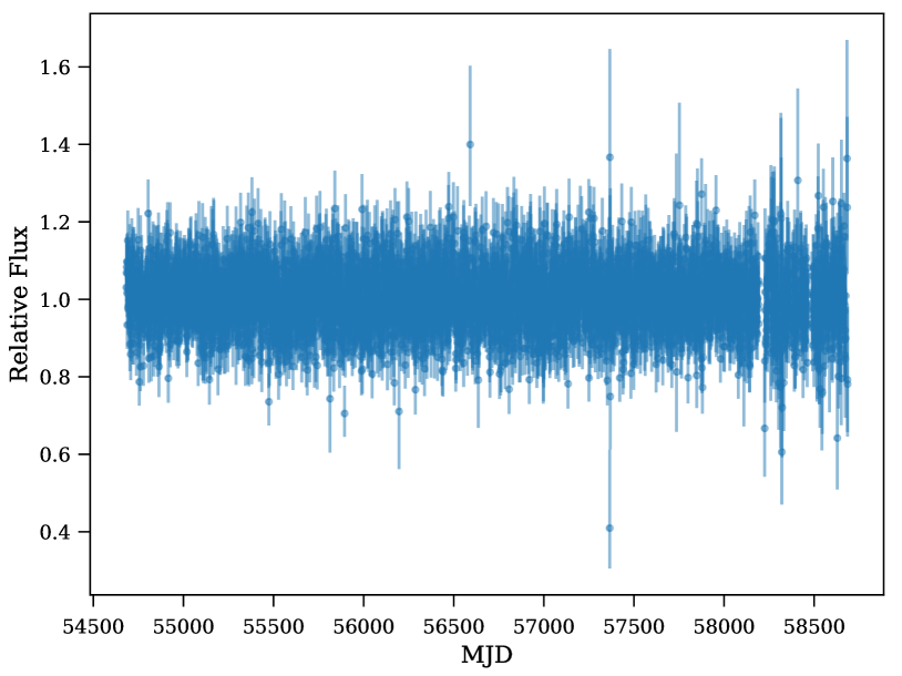
Figure 1: Light curve for Geminga with 1-day resolution. Days with exposure below threshold are not depicted, and the source is otherwise strongly detected on each interval.

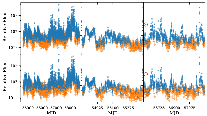
Figure 2: Light curve for 3C 279. The upper panels show estimates made with the background fixed to its average value ($\beta=0$), while the lower panels are computed with a profile likelihood maximized with respect to $\beta$. Upper limits (orange arrows) are shown for days with TS $<9$. The middle and right panels focus on 700-day intervals beginning MJD 54750 and 56550, respectively. The measurement indicated by the red circle corresponds to an M1.5 solar flare (see main text), which is confused with the blazar. The profile likelihood correctly assigns this flux to the background.

3 Weight Computation, Exposure Calculation, and Software

For all examples presented here, we use about 10 years of Pass 8 (Atwood et al., 2013) Fermi-LAT data, selected to have reconstructed arrival directions within 2$\arcdeg$ (typically), 5$\arcdeg$, or 10$\arcdeg$ (as noted) of the source. We compute photon weights using the pointlike (Kerr, 2010) application and a model of the sky based on the FL8Y source list.

To compute the expected source rates in a given time interval, it is necessary to know the exposure—the product of effective area and integration time—towards the source. In a typical likelihood analysis, e.g. one carried out with the Fermi Science Tool gtlike, the exposure is calculated as a function of energy and position and spectral analyses are carried out over large (say 20$\arcdeg$) ROI. Because we are using the products of such an analysis and restricting attention to a small ROI, we are able we evaluate the exposure only at the position of the source. We further use a spectral model (by default a power law with spectral index $-2.1$) to average the effective area over energy. In principle, better results are obtained by using the correct spectral model for the source, but in practice, we find little difference compared to this omnibus model. We compute the exposure directly from the 30-s intervals tabulated in the FT2 file distributed by the Fermi Science Support Center.

We have made the software to compute exposure and to perform all of the analyses presented here available in the package godot. In particular, godot provides routines for the selection of LAT data on a variety of time scales, e.g. contiguous viewing periods or uniform time bins, and aggregating the data and exposure into arbitrarily-sized cells as required for further analysis. Some care has been taken to optimize the performance. Routines for computing data cells using Solar System barycentric time, critical for identifying very short period binaries, are also provided (see §5).

Therefore, in summary, users wishing to try out the techniques described here should (1) install the Fermi Science Tools and godot; (2) adapt an existing sky model (e.g. 4FGL) or develop a new one using gtlike if the source of interest is not in the sky model (3) use the sky model and the gtsrcprob Science Tool to produce photon weights for all sources of interest; (4) use the applications in godot to apply retrospective likelihood analysis.

4 Light Curves

A light curve is a time series of point estimators of the intensity of emission received from a given source. From Eq. 2, we see we can obtain such estimators by dividing the data into suitable segments $P_{k}$ and maximizing $\mathcal{L}_{k}(\alpha_{k},\beta_{k})$. We can estimate confidence intervals by applying a uniform prior (restricted to positive values, $\alpha_{k},\beta_{k}$$>$$-1$) and computing the range which encloses a specified fraction of the posterior distribution for $\alpha_{k}$/$\beta_{k}$ (68% for 1 $\sigma$ error flags) . In determining $P_{k}$, for practicality, we restict attention to segments of $\geq$30 s, which is the interval at which the spacecraft (S/C) position and orientation are recorded in standard data products. Even the brightest sources, with fluxes (E $>$ 100 MeV) of $10^{-5}$ to $10^{-4}$ ph cm^-2 s^-1, are barely detectable in such short segments, and a more useful interval is the roughly 20 minutes during which the source is in the LAT field-of-view during a typical (zenith-pointed) orbit. Besides gamma-ray bursts, only a few sources have been observed to show variability at or below the orbital time-scale, e.g. flaring blazars like 3C 279 (Ackermann et al., 2016), 3C 454.3 (Abdo et al., 2011a), and 4C$+$21.43 (Tanaka et al., 2011)—see also Meyer et al. (2019) for a more general analysis; the third observed periastron passage of PSR B1259$-$63 (Johnson et al., 2018); and the Crab Nebula (e.g. Buehler et al., 2012; Abdo et al., 2011b). Accordingly, analyses typically use longer (1 day, 1 week) bins. But by selecting a longer time-scale for averaging, there is risk of washing out rapid variability. As we will show below, adopting relatively short bins for the likelihood analysis and using aggregating techniques like Bayesian blocks or multi-scale filtering is an effective means of probing a wide range of time scales.

4.1 Examples and Profile Likelihood

Here, we consider two sources as examples. First, we analyze the Geminga pulsar (PSR J0633$+$1746), the second-brightest pulsar in the Fermi sky (Abdo et al., 2010). To date, it is not known to show any variability, and it thus makes a good test source for probing systematic errors in the method. To estimate its light curve, we take $\alpha_{k}$ as constant over a single day, and we fix $\beta=0$. To avoid measurements with large uncertainty, we exclude days whose exposure is $<$10% of the mean. The resulting estimators (maximum likelihood with 1 $\sigma$ error bars) appear in Figure 1. As expected, they are consistent with $\alpha_{k}=0$ to a high degree of accuracy. A failure in one of the Fermi solar panel array drives (MJD 58194) resulted in a revised S/C rocking profile and less homogeneous exposure on few-week timescales. The resulting inhomogeneity in measurement precision following this date is apparent. Nonetheless, the uncertainties are accurately estimated and the error-normalized measurements follow an outlier-free unit normal distribution.

As a second example, we consider the highly variable blazar 3C 279 and as above we compute daily estimators of the flux density. Unlike Geminga, 3C 279 is not always bright enough to detect every day, and we report upper limits when the TS$\equiv 2\times[\log\mathcal{L}(\hat{\alpha_{k}})-\log\mathcal{L}(-1)]$ (with $\hat{\alpha_{k}}$ the maximum likelihood estimator) is $<9$. The light curve, displayed in Figure 2, shows relatively typical (albeit intense) flares lasting multiple days, in keeping with causality arguments about source size. The leftmost panels shows the entire data range, while the right panels focus on shorter, 700-day intervals to show more structure. In the right panel, one measurement, indicated with a red circle at MJD 56576.5, seems to be an “orphan” flare surrounded by upper limits. Such variability is faster than expected, and indeed this point is actually due to a behind-the-limb solar flare producing bright MeV–GeV emission, a fast coronal mass ejection, and solar energetic particles (Ackermann et al., 2017). At the time of this flare, the sun was only 2$\arcdeg$ from 3C 279, and their emission is confused, leading to the incorrect flux estimator. In the bottom panels, we show the same light curves obtained by maximizing the profile likelihood, $\log\mathcal{L}(\alpha_{k},\hat{\beta_{k}}(\alpha_{k}))$, the likelihood maximized with respect to the background for each value of $\alpha_{k}$. Because the extended solar emission over the ROI “looks” very much like an additional, flat background component, the new degree of freedom absorbs the contribution from the solar flare and the best-fit flux value and TS drop from $F/F_{\mathrm{mean}}=4.6$ and TS$=342$ to $F/F_{\mathrm{mean}}$=0 and TS$=0$, i.e. a non-detection. In general, the profile likelihood requires modestly more computation and reduces measurement precision. Here, the typical TS is halved, though this depends on ROI size (see Fig. 9). But it clearly provides an important check on the $\beta=0$ assumption, and future work could improve measurement precision by adopting a more physical prior on $\beta$.

4.2 Bayesian Blocks

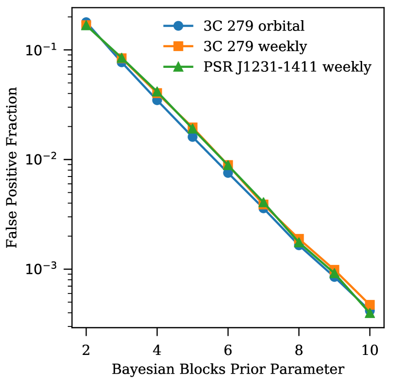
Figure 3: Simulations showing the false positive rate (defined as the number of blocks in excess of one divided by the total number of cells) as a function of the prior parameter $\gamma$.

Bayesian blocks (hereafter “BB”, Scargle, 1998) is a method of partitioning a data set comprising $N_{c}$ elementary cells into $N_{b}$ longer blocks that maximize the posterior probability according to some model of variability. Most simply, this model is piecewise constant, and the method can be viewed as a way of compressing cells into blocks of nearly-constant emission level. The level of compression is controlled by the priors adopted for the variability model, and in the piecewise constant model it can be taken as a prior on $N_{b}$. A commonly-used prior, which we adopt, takes the form $\pi(N_{b})\propto N_{b}^{-\gamma}$, penalizing additional blocks with “strength” controlled by $\gamma$.

With this prior, or any prior such the log posterior for independent data segments is additive, there is an efficient $\mathcal{O}(N_{c}^{2})$ dynamic programming algorithm for determining the optimal data partition (Scargle et al., 2013). This approach is particularly attractive when paired with a fast likelihood algorithm, in which case it enables multi-scale variability analysis by providing the algorithm with many very short data cells and allowing it to “detect” variability via a preference for one or more change points. If the optimal partition has only one block, there is no variability. In the presence of variability, the algorithm automatically and optimally divides the data up such that the measurement precision is high while fast variability is not oversmoothed by binning.

The BB algorithm starts with a single cell (which is already the optimal partition!) and with each iteration adds a new cell and identifies a new optimal partition. Because there will be $N_{c}$ iterations, each iteration must be completed in $\mathcal{O}(N_{c})$ operations to achieve the $\mathcal{O}(N_{c}^{2})$ complexity. Generally, the $j$th iteration will require evaluation of $j$ new fitness functions on partitions containing on average $j/2$ cells and $\mathcal{O}(j)$ photons. If the fitness function is independent of the partition length, e.g. the Poisson likelihood for total counts, the $j$ $\mathcal{O}(1)$ operations satisfy the $\mathcal{O}(j)$ complexity for the iteration. But evaluating Eq. 2 for a typical cell requires $\mathcal{O}(j)$ operations, giving $\mathcal{O}(j^{2})$ complexity for the iteration and $\mathcal{O}(N_{c}^{3})$ overall. To avoid this, we have implemented a caching scheme in which we first analyze the log likelihood for each cell to determine the location of its maximum ($\hat{\alpha}$) and the points at which it has decreased by a given amount (by default 30). We then evaluate and store the likelihood on a grid of points over this range (by default $N_{pt}=200$), and we can optimize the likelihood for the sequence of blocks simply by combining these grids and finding the maximum. In this way, evaluation of the fitness function for the sequence requires $\mathcal{O}(N_{c}\times N_{pt})$ operations. This scheme is implemented in godot and used for the the following analyses.

Sensitivity to variability, e.g. the false positive and false negative rate, is governed by the prior. Our choice of $N_{b}^{-\gamma}$ reduces the log likelihood by $\gamma$ for each block (degree of freedom), enforcing parsimony. Generally, $\gamma$ must be carefully chosen to match the properties of the specific data set. When the individual data cells are sufficiently large that the Central Limit Theorem applies, the log likelihoods will follow $\chi^{2}$ distributions. Then, the false positive rate (creation of a spurious change point) will depend only on $\gamma$ and $N_{c}$ and not on the properties of the source in question. Then $\gamma$ can be trivially tuned to give the desired false positive rate. On the other hand, if some cells have only a few photons of low weight, as might be the case for those comprising single Fermi-LAT orbits, the false positive rate would depend sensitively on the exact exposure. In this case, simulations are useful in determining the ideal prior.

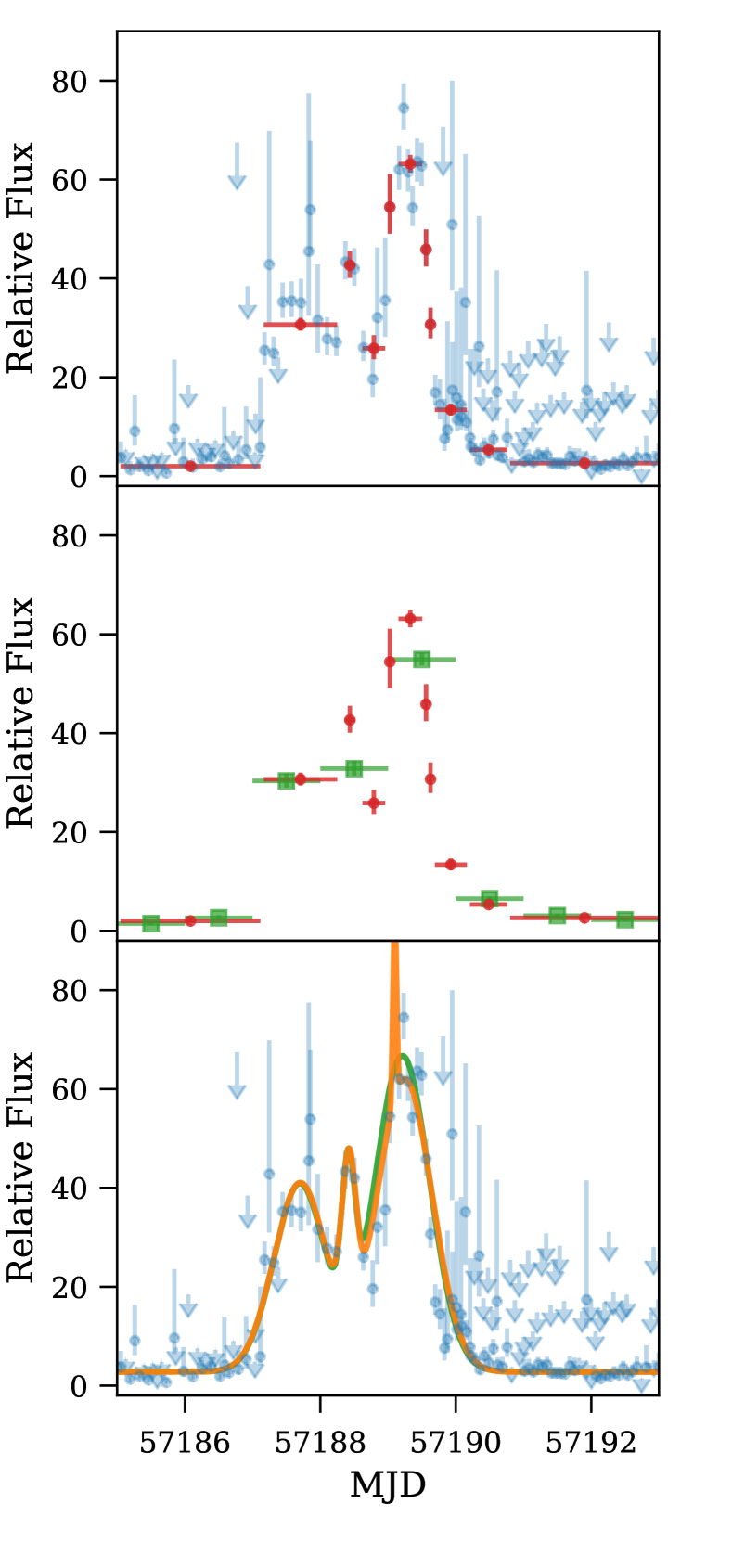
Figure 4: Light curve for a single 3C 279 flare. (Top) The raw likelihood fits from individual orbits are shown in blue; the typical duration of the data acquired during an orbit is too narrow to illustrate. Blocks obtained with the BB algorithm are shown in red, with horizontal errors indicating the block extent and vertical errors the flux uncertainty. (Middle) BB shown in red as in top. The green points indicate likelihood fits performed with 1 d integrations, with flux density errors too small to see. (Bottom) As top, blue points show likelihood fits from individual orbits, while two analytic models with 3 (green) and 4 (orange) gaussian are fit using the orbital likelihoods.

We have carried out such simulations by re-distributing photons randomly amongst cells according to their computed source rates and then applying the BB algorithm. (We have included this simulation capability in godot.) Some of our test cases are illustrated in Figure 3 and include uniform bins and steady sources (PSR J1231$-$1411, one-week bins), uniform bins with strongly variable sources (3C 279, one-week bins), and nonuniform, very short bins with strongly variable sources (3C 279, orbital/$\sim$20-minute bins). Interestingly, we find that the false positive rates for all test cases closely follow the exponential shape of the prior, regardless of fluctuation level of the cells. The rate is roughly $0.8\,\exp(-0.8\gamma)$, reminiscent of the aymptotic null distribution of the $H$ statistic (Kerr, 2011), which similarly involves a maximization over $\chi^{2}$ variables. This calibration allows a sensible choice of $\gamma$ for any data set. Many typical analyses are covered by a dynamic range of $\sim$1000, so selecting $\gamma=8$ with a false positive rate $\sim$0.001 works well. Wider dynamic ranges (e.g. searches for sub-day variability in the full Fermi data set) require $\gamma\geq 10$.

To summarize this discussion, the combination of a fast likelihood and Bayesian blocks is a powerful, universal method for detecting variability on a wide range of time scales. We demonstrate this with an analysis of a bright flare from 3C 279, using data from MJD 57185 to 57193. As cells, we select photons from contiguous exposure intervals, typically about 20 m every 3 hr (two orbits), though exposure interruptions from passage through the South Atlantic Anomaly can produce two shorter exposures. In this case, a Target of Opportunity request resulted in several days of pointed mode observations, so in total we have 146 cells over the 8 d of data. Accordingly we choose $\gamma=8$ for the prior. The top panel of Figure 4 shows the results for both the flux density estimates from individual cells (blue) and the resulting BB partition (red). In its brightest state, 3C 279 is strongly detected in single orbits, while observations outside of the flare yield only upper limits. The BB algorithm accurately identifies all of the major variability evident in the high time resolution data, including a sharp sub-flare between the two broad peaks and the very strong peak lasting one single orbit. Moreover, by aggregating the data in the off-peak intervals, it provides good estimates of the quiescent flux. By contrast, the middle panel shows the same data set but binned into 1 d cells (green), a common choice for monitoring blazars. The main peak is under resolved, the rapid variability between and within the peaks is smoothed away, and quiescent portions are broken up over multiple bins.

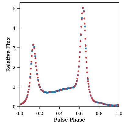
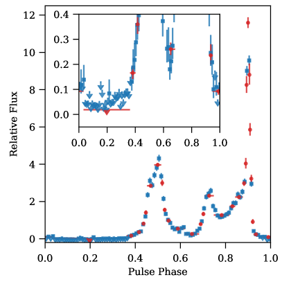
Figure 5: Pulse profiles for Geminga (left) and PSR J1231$-$1411 (right). Blue points give maximum likelihood estimates in 100 uniform phase bins, while red symbols indicate the BB partition. The inset emphasizes the stringent off-peak upper limit.

4.3 Waveforms

Although we have concentrated on piecewise models, we include here an example of fitting an analytic shape using the orbital-time scale likelihood. At these time scales, the flux density estimators are highly non-gaussian, so it is better to use the full likelihood rather than, e.g., using least squares to fit a functional form to the estimators. Applications might include characterizing rise and fall times of flares, investigating the significance of transient features, and model selection. Here, we investigate the presence of fast flares by first fitting, using maximum likelihood, a simple three-gaussian model to the apparent three-peak structure of the flare. The resulting model appears in green in the bottom panel of Figure 4, along with the direct orbital measurements. These orbital measurements appear to indicate an un-modelled fast flare at the onset of the third peak. To test the significance of this feature, we add and optimize a fourth gaussian, which improves the log likelihood by 20, indicating it is likely to be a real feature. Although this example is entirely ad hoc, we direct the reader to Meyer et al. (2019) for physically motivated modelling of fast variability in 3C 279 and other blazars.

4.4 Pulse Profiles

The flux density of pulsars as a function of rotational phase (also widely referred to as “light curves”, but here called pulse profiles for clarity) are particularly well suited to this method. Indeed, because the rotational time scale is so well separated from typical times over which exposure and backgrounds vary, any background variation is common across pulse phase bins and does not affect pulse profile estimation. Pulse profiles are typically presented as histograms, either of Stokes parameters recorded by radio telescopes or of photons by high-energy experiments. Consequently, we adopt the piecewise-constant formulation for the source intensity. However, we note that unbinned analytic models, e.g. truncated Fourier expansions, gaussians, lorentzians, etc. can also be used to model $\alpha$ (see §4.3).

The likelihood formalism here has several advantages over previous approaches. The most suitable direct comparison are the weighted photon histograms presented in Abdo et al. (2013), which have estimators for the background level and bin uncertainty; these quantities are both estimated from the global weights distribution, and certain artifacts appear where the bin distribution differs substantially, e.g. a narrow off-pulse or a bright peak. In contrast, the likelihood method here yields a direct estimate both of the pulsar flux density and of its uncertainty based entirely on the “local” distribution of photons. It is, in essence, a fixed-shape but bona fide spectral analysis of each bin. (See Guillemot & Kerr (2019) for a more complete treatment of phase-resolved spectroscopy.)

Moreover, this approach admits a fitness function appropriate for the BB algorithm. Previous analyses applying BB to pulse profiles have either used only unweighted counts (e.g. Lande, 2014), losing sensitivity, have used less powerful statistics like the $F$-test as a fitness function (Caliandro et al., 2013), or require a transformation of the raw data to a more suitable form (Ajello & et al., 2019). As in the previous section, we can use an intrinsically high resolution, say 1000 phase bins, for computation of the data partition, while keeping a modest resolution, say 100 phase bins, for a descriptive presentation. As before, we use simulations to determine the correct BB prior to give $\sim$1 partition in the case of uniform phase data with the same distribution of weights. (We remind the reader here that, in order to enforce the periodic boundary condition of a pulse profile, the BB algorithm should be applied to three full rotations, with the data representation taken from the partition of the central rotation.)

For our first example, we again use the Geminga pulsar, and the now-familiar scheme appears in the left panel of Figure 5. The blue points result from a “typical” pulse profile of 100 uniform phase bins, while the red points are a BB partition based on 1000 bins. The analyis shows the ad hoc binning has underresolved the two peaks, but also clearly demonstrates that there is no fine structure in the pulse profile. As a second example, we consider the bright millisecond pulsar J1231$-$1411 (Ransom et al., 2011), which has one of the sharpest peaks of Fermi pulsars. The 100-bin profile dramatically underresolves the main peak, while at the same time overresolves the off-pulse. By correctly aggregating the bins with the BB method, we capture both the milliperiod structure in the bright peak and simultaneously obtain an optimal definition of the off-pulse region and a stringent upper limit on its amplitude of $<1.6\%$ of the mean flux. The fine-grained likelihood and BB partition together capture all of the information in the pulse profiles in a simple visual representation.

5 Power Spectra

A small but important class of LAT sources include $\gamma$-ray binaries such as LS I $+$61$\arcdeg$ 303 and LS 5039. These sources, with an O or Be-type stellar companion, are known as microquasars and are strong emitters of $\gamma$ rays modulated at the orbital period. In some systems, the nature of the compact object is still unknown and may either be a neutron star or a stellar-mass black hole. In most models the orbital modulation is governed by the dependence of Doppler boosting on the viewing angle; see Dubus (2013) for an overview.

Because $\gamma$-ray binaries are exceedingly scarce, the discovery of new systems plays an important role in understanding their nature, and so motivates the development of more sensitive search techniques. Corbet et al. (2007) devised a method of “exposure weighting” to measure power spectra in data sets with very inhomogeneous exposure, and later incorporated photon weights (Corbet & Kerr, 2010) to increase the sensitivity. These developments were key to the discovery of new $\gamma$-ray binaries such as 1FGL J1018.6$-$5856 (Ackermann et al., 2012) and CXOU J053600.0$-$673507 in the LMC (Corbet et al., 2016). Here, we demonstrate a connection between these formulations and the methods developed here. The new formalism puts the search methods on a rigorous footing, offers an analytic normalization for the control of trials factor, and in some cases improves sensitivity (e.g. §6).

We begin by expanding the normalized flux densities for the source and background over time using a Fourier series:

$$\alpha(t)= \sum_{l=1}^{N}\alpha_{cl}\cos(l\phi)+\alpha_{sl}\sin(l\phi)$$

$$\beta(t)= \sum_{l=1}^{N}\beta_{cl}\cos(l\phi)+\beta_{sl}\sin(l\phi)$$

with the sum extending up to the Nyquist frequency for the data and $\phi\equiv 2\pi t/T$ with $T$ the length of the data set. In the following derivation, we assume that the modes are independent and for brevity concentrate on a single source and background mode, taken without loss of generality to be $\alpha_{c1}$ and $\beta_{c1}$. In most analyses, this assumption of independence is a good one, but we assess the effect of the window function further below. Now, defining $(1-w_{i})\equiv\bar{w}_{i}$, Eq. 2 becomes

$$\log\mathcal{L}= \sum_{k}\bigg{[}\sum_{i\in k}\log\big{[}1+w_{i}\big{(}\alpha_{c1}\cos(\phi_{k})+\ldots\big{)}+\bar{w}_{i}\big{(}\beta_{c1}\cos(\phi_{k})+\ldots\big{)}\big{]}\bigg{]}$$

$$-S_{k}[\alpha_{c1}\cos(\phi_{k})+\ldots]-B_{k}[\beta_{c1}\cos(\phi_{k})+\ldots]$$

This expression can be further simplified if $\alpha_{c1}w_{i}\ll 1$ and/or $\beta_{c1}\bar{w}_{i}\ll 1$. $\alpha$ describes the fractional modulation associated with a mode, so can be small when either the overall modulation relative to the source intensity is low, or when a complex waveform requires small contributions from many modes. As an example, a typical low-order mode of a pulsar waveform might have $\alpha\sim 0.1$. The weights $w_{i}$ are small when the source is faint relative to the background, which is the case for almost all Fermi sources. Thus, the product $\alpha_{c1}w_{i}$ is almost always $\ll 1$. For background photons due to other sources, similar arguments apply. For strong diffuse background sources, $\bar{w}_{i}\approx 1$ is typical, but such backgrounds are not strongly modulated, so $\beta_{c1}\ll 1$ is an excellent approximation. Residual particle background, on the other hand, may be strongly modulated as Fermi orbits the earth, but the fraction of such events that survive background rejection is small such that $\bar{w}_{i}\ll 1.$ Thus, we expand the logarithm and suppress subscripts for other modes to find

$$\log\mathcal{L} \approx\sum_{k}\sum_{i\in k}\cos(\phi_{k})\bigg{[}w_{i}\alpha+\bar{w}_{i}\beta-\alpha S_{k}-\beta B_{k}\bigg{]}-\cos^{2}(\phi_{k})\bigg{[}\frac{1}{2}w_{i}^{2}\alpha^{2}+w_{i}\bar{w}_{i}\alpha\beta+\frac{1}{2}\bar{w}_{i}^{2}\beta^{2}\bigg{]}$$

$$\equiv\sum_{k}\cos(\phi_{k})\bigg{[}W_{k}\alpha+\bar{W}_{k}\beta-\alpha S_{k}-\beta B_{k}\bigg{]}-\cos^{2}(\phi_{k})\bigg{[}\frac{1}{2}WW_{k}\alpha^{2}+W\bar{W}_{k}\alpha\beta+\frac{1}{2}\bar{W}\bar{W}_{k}\beta^{2}\bigg{]}$$

$$\equiv\alpha\langle W-S\rangle_{c}+\beta\langle\bar{W}-B\rangle_{c}-\frac{1}{2}\alpha^{2}\langle\langle WW\rangle\rangle_{c}-\alpha\beta\langle\langle W\bar{W}\rangle\rangle_{c}-\frac{1}{2}\beta^{2}\langle\langle\bar{W}\bar{W}\rangle\rangle_{c},$$

where we have grouped weights in the same cell into the series $W_{k}$ and $\bar{W}_{k}$ and denoted the cosine-weighted sums over cells with e.g. $\sum_{k}\cos(\phi_{k})W_{k}\equiv\langle W\rangle_{c}$ and $\sum_{k}\cos^{2}(\phi_{k})W\bar{W}_{k}\equiv\langle\langle W\bar{W}\rangle\rangle_{c}$. (We suppress these subscripts until needed.) Finally, if we differentiate the likelihood with respect to $\alpha$ and $\beta$ and solve the resulting system of equations, we find the maximum likelihood estimators

$$\hat{\alpha}=\frac{\langle\langle\bar{W}\bar{W}\rangle\rangle\langle W-S\rangle-\langle\langle W\bar{W}\rangle\rangle\langle\bar{W}-B\rangle}{\langle\langle WW\rangle\rangle\langle\langle\bar{W}\bar{W}\rangle\rangle-\langle\langle W\bar{W}\rangle\rangle^{2}} \hat{\beta}=\frac{\langle\langle{W}{W}\rangle\rangle\langle\bar{W}-B\rangle-\langle\langle W\bar{W}\rangle\rangle\langle W-S\rangle}{\langle\langle WW\rangle\rangle\langle\langle\bar{W}\bar{W}\rangle\rangle-\langle\langle W\bar{W}\rangle\rangle^{2}}.$$ (3)

On the other hand, if we assume that $\beta=0$ (steady background) or $\alpha=0$ (steady source), we obtain the simple estimators

$$\hat{\alpha_{0}}=\frac{\langle W-S\rangle}{\langle\langle WW\rangle\rangle} \hat{\beta_{0}}=\frac{\langle\bar{W}-B\rangle}{\langle\langle\bar{W}\bar{W}\rangle\rangle}.$$ (4)

Finally, we can insert these estimators back into the second-order likelihood to find the change in the log likelihood relative to the no-modulation null case, $\delta\log\mathcal{L}=\log\mathcal{L}(\alpha=\hat{\alpha},\beta=\hat{\beta})-\log\mathcal{L}(\alpha=\beta=0)$:

$$2\,\delta\log\mathcal{L}\approx P_{c}\equiv\frac{\langle\langle\bar{W}\bar{W}\rangle\rangle\langle W-S\rangle^{2}-2\langle\langle W\bar{W}\rangle\rangle\langle W-S\rangle\langle\bar{W}-B\rangle+\langle\langle WW\rangle\rangle\langle\bar{W}-B\rangle^{2}}{\langle\langle WW\rangle\rangle\langle\langle\bar{W}\bar{W}\rangle\rangle-\langle\langle W\bar{W}\rangle\rangle^{2}}$$ (5)

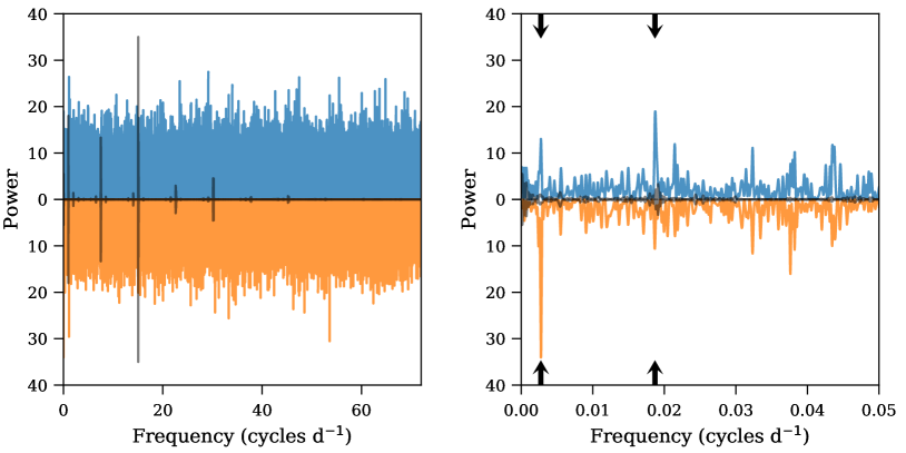
Figure 6: The power spectrum of Geminga. (left) The full power spectrum is shown up to the limiting frequency of 72 cycles d^-1, with the background-fixed estimator ($P_{0}$) shown in orange below the x-axis and the profile likelihood ($P_{1}$) estimator in blue, above. The black trace gives the window function for the exposure (see main text). (right) A focus on low-frequency signals reveals the only two systematic effects. Power in $P_{0}$ at a period of 1 yr (left black arrows) is likely caused by the sun, while power in $P_{1}$ at the S/C precessional frequency (right arrows) is probably induced by small inaccuracies in the exposure correction.

We have defined $P_{c}$, the estimator for the power in the “cosine” mode, and there are analogous estimators and an expression for $P_{s}$ with sine-weighted sums. Combining these quantities gives two estimators for the power spectrum, $P_{0}$ with the background fixed to its time-averaged value ($\beta(t)=0$), and $P_{1}$ with it fixed to its maximum likelihood value:

$$P_{0} =\frac{\langle W-S\rangle_{c}^{2}}{\langle\langle WW\rangle\rangle_{c}}+\frac{\langle W-S\rangle_{s}^{2}}{\langle\langle WW\rangle\rangle_{s}},$$ (6)

$$P_{1} =P_{c}+P_{s}-\frac{\langle\bar{W}-B\rangle_{c}^{2}}{\langle\langle\bar{W}\bar{W}\rangle\rangle_{c}}-\frac{\langle\bar{W}-B\rangle_{s}^{2}}{\langle\langle\bar{W}\bar{W}\rangle\rangle_{s}}.$$ (7)

By Wilke’s Theorem, both of these quantities are distributed as $\chi^{2}_{2}$ in the null hypothesis. We thus see that this estimator, with a mean of 2, satisfies Leahy normalization (Leahy et al., 1983). The numerators of $P_{0}$, $\langle W-S\rangle_{c}^{2}$ and $\langle W-S\rangle_{s}^{2}$, are the exposure-weighted power spectrum estimators of Corbet et al. (2007), so we see that the maximum likelihood estimator $P_{0}$ is a generalization that is naturally Leahy normalized. To this, $P_{1}$ adds the ability to absorb background fluctuations. Moreover, this formulation suggests the evalulation of these sums using the Fast Fourier Transform, and indeed, by using suitable identities, $P_{0}$ and $P_{1}$ can be evaluated for all relevant frequencies by evaluating 2 and 5 FFTs, respectively. For $P_{0}$, this formulation is

$$P_{0}(\nu)/2= \frac{\mathrm{Re}[\mathcal{F}(W-S)(\nu)]^{2}}{\mathrm{Re}[\mathcal{F}(W^{2})(2\nu)+\mathcal{F}(W^{2})(0)]}$$ (8)

$$- \frac{\mathrm{Im}[\mathcal{F}(W-S)(\nu)]^{2}}{\mathrm{Re}[\mathcal{F}(W^{2})(2\nu)-\mathcal{F}(W^{2})(0)]},$$

with $\mathcal{F}$ denoting a Fourier transform. The expression for $P_{1}$ is too lengthy to include here, and we refer the reader to the implementation in godot for details. These formulations yield a substantial computational benefit, and as we show in the examples below, enable construction of power spectra with time scales as short as 2 minutes. The evaluation time is perhaps 10 s on a modest CPU.

We now give a series of examples demonstrating the manifestation of various types of source signal in power spectra computed according to Eqs. 6 and 7. As before we first test for systematics by considering sources lacking bona fide astrophysical variability on these time scales. Such sources should be characterized by uniform power spectra, and the departure from such a spectrum indicates a possible discovery, e.g. a line in the power spectrum for a periodic source, a slightly wider feature for a quasi-periodic oscillation, or colored noise for the stochastic variability of an active galactic nucleus (AGN). First, we consider Geminga. The pulsed emission (Fig. 5) is modulated at the spin period of 237 ms, far faster than the time scales we probe here. We binned the exposure into 300-s intervals, which allows computation of frequencies of up to 72 d^-1, or 20 minutes. (Although the Nyquist frequency for 300-s sampling is 144 d^-1, the FFT formulation in Eq. 8 requires the evaluation of FFTs up to twice the maximum frequency of interest, so only the lower half of the Nyquist band is available.) The power spectra, obtained both with the fixed- ($P_{0}$) and free-background ($P_{1}$) assumptions, appear in Figure 6. There are about $10^{6}$ independent frequency samples in this spectrum, and it is almost perfectly white,. Moreover, the samples follow the expected $\chi^{2}_{2}$ distribution, and the maximum value of $P=27.8$ is expected to occur by chance in a sample this large with frequency $\mathcal{O}(1)$.

This nearly featureless spectrum is remarkable considering that the exposure varies periodically on a wide range of scales, as does the background. The “window function”, the power spectrum of the exposure towards Geminga, appears as a black trace superimposed on the power spectrum, arbitrarily scaled such that the maximum power near the S/C orbital frequency ($f_{sc}=15.1$ d^-1, about 95.4 minutes) is 35. The window function has strong variation at the S/C precessional frequency ($f_{prec}=0.019$ d^-1, about 53.4 d) and at $f_{sc}$ and its harmonics. The background from residual particles, which contributes variability but does not influence the window function, varies principally on 1-day time scales, as this is roughly the time required to make a complete circuit of the magnetosphere. We refer the reader to the FSSC documentation for a more complete description of variability time scales.

The small signal in $P_{0}$ at 1 yr^-1 ($f=2.7\times 10^{-3}$ d^-1) is likely associated with the annual passage of the sun, a modestly strong and extended $\gamma$-ray source, by Geminga, at ecliptic latitude $-5.4^{\circ}$. Because the sun’s extended emission is largely degenerate with the steady background, the contamination vanishes when using the profile likelihood ($P_{1}$) estimator for the power spectrum. On the other hand, the $P_{1}$ signal at $f_{prec}$ likely results from very small inaccuracies in the exposure calculation.

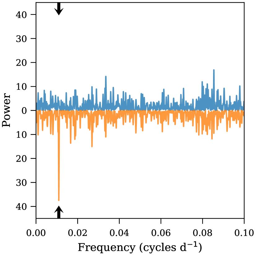
Figure 7: The power spectrum for 3FGL J0823$-$4205c, focused on low frequencies. The lower, orange trace, $P_{0}$, shows a strong peak at 0.011 d^-1 (black arrows; 4 cycles per year, see main text) while the upper blue trace, $P_{1}$, shows no signal here or at high frequencies (not pictured).

Next, we consider 3FGL J0823.3$-$4205c, a much weaker source that lies only 3$\arcdeg$ away from Vela (PSR J0835$-$4510), the brightest persistent GeV $\gamma$-ray source. The power spectrum is featureless at all frequencies save for the portion shown in Figure 7, which reveals a signal in $P_{0}$ at 4 yr^-1 ($f=0.011$ d^-1). This artefact stems from the four-fold symmetry of the Fermi-LAT point-spread function. Over the course of a year, the typical azimutal angle at which Vela is viewed completes a full rotation. The concomitant rotation of the projected PSF on the sky causes the background contribution from Vela to vary annually, and the four-fold symmetry leads to the 4 yr^-1 signal. As with the solar contamination of Geminga, $P_{1}$ is insensitive to this effect.

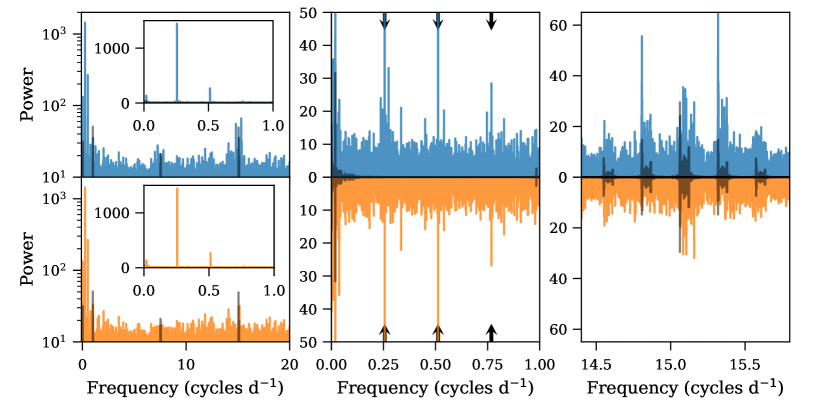
Figure 8: The power spectrum of LS 5039. The top panels show the “raw” spectrum (blue), while the bottom panels (orange) show a version with time-domain signal subtraction, which reduces spectral leakage. (left) The spectrum over a large section of bandwidth, with spectral leakage visible at the S/C orbital frequency $f_{sc}=15.1$ d^-1. The inset shows the strength of the LS 5039 modulation in the fundamental and first harmonic of the orbital frequency $f_{ls}=0.26$ d^-1. (middle) A closer view of spectral leakage around $f_{ls}$ and its harmonics (marked with arrows). The leakage is essentially a copy of the window function produced by the Fermi orbit. (right) Spectral leakage from $f_{ls}$ to $f_{sc}$. The window function is shown in black and is reproduced, scaled, and shifted by $f_{ls}$ and $2f_{ls}$, respectively, to demonstrate the origin of the leakage. The time domain method removes almost all of the power associated with leakage from the fundamental, while the broad peak at $f_{sc}$, due to low-frequency variation of LS 5039, remains, as does power associated with $2f_{ls}$.

These tests of steady sources are important for the discovery of modulations, i.e. excess power for an object with an otherwise-white underlying spectrum. We now consider characterization of sources with known modulation and the effects of the window function on its measurement. Quite generally, power intrinsic to a given frequency will be redistributed over the observed band; specifically, this redistribution is given by the convolution of the true power spectrum with the Fourier transform of the window function. For Fermi, with its discontinous viewing periods, this manifests as a series of sinc²-like peaks clustered around $f_{prec}$, $f_{sc}$, and their harmonics (see Figures 6 and 8).

To illustrate the various features, we consider the power spectrum of LS 5039, a strong $\gamma$-ray binary (e.g. Abdo et al., 2009a) with an orbital frequency $f_{ls}=0.26$ d^-1 (period 3.9 d). The power spectrum appears in Figure 8 and is dominated by the orbital modulation, clearly visible in the upper left hand panel, with large power at $f_{ls}$ and $2\times f_{ls}$. This power “leaks” to other frequencies “through” the window function, and this is clear from the main panel showing frequencies up to 20 d^-1. The upper blue trace is the raw power spectrum (Eq. 6), and there is clear power in excess of the white noise floor near $f_{sc}$ and $f_{sc}/2$ ($\sim$15.1 d^-1 and $\sim$7.5 d^-1), where the window function also has power. The middle panel highlights spectral leakage around $f_{ls}$ and its harmonic; a single line has become a forest of power. Finally, in the upper right panel, we highlight the power that has appeared near $f_{sc}$. True low-frequency power associated with secular variation of LS 5039 is convolved with the window function, producing a broad peak at $f_{sc}$. On the other hand, the two LS 5039 peaks, being essentially delta functions, produce an exact copy of the window function at $f_{sc}\pm f_{ls}$ and $f_{sc}\pm 2f_{ls}$. To illustrate this, we have reproduced the window function and shifted it to these frequencies.

To reduce this spectral leakage, it is possible to remove the strong orbital modulations in the time domain before evaluating Eq. 6, and then restoring the power afterwards. We do this by directly fitting a sinusoid at $f_{ls}$ using Eq. 2 with the 300s segments and updating the predicted counts $S_{k}$ with the modulation before computing $P_{0}$ and $P_{1}$. These results appear in the lower orange traces. Generally, the power spectrum is unchanged in regions where the window function is minimal (exposure variations washed out), but substantially improved near problematic frequencies. This approach is critical in the analysis of strongly pulsed sources; see, e.g., the analysis of an ultraluminous X-ray pulsar (Wilson-Hodge et al., 2018).

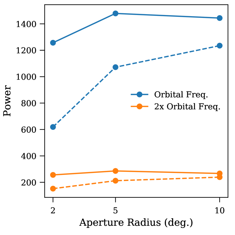
Figure 9: The power obtained at the fundamental (blue) and first harmonic (orange) orbital frequency for LS 5039 when using $P_{0}$/Eq. 6 (solid) and $P_{1}$/Eq. 7 (dashed).

Because the orbital modulation provides a clear way to distinguish the source from the background, LS 5039 provides a nice way to study the dependence of our two power spectrum estimators $P_{0}$ (Eq. 6, with constant background), and $P_{1}$ (Eq. 7, with variable background) on ROI size. Generally we expect two effects: (1) a larger ROI should contain more source photons than a smaller one, until the ROI fully encloses the PSF; (2); the background will be degenerate with the source intensity until the ROI is large enough to “resolve” the source. Kerr (2011) showed that for most Fermi pulsars a 2$\arcdeg$ ROI was sufficient to garner most of the signal, as even though the LAT PSF is larger than this at low energies, the signal-to-background ratio drops rapidly outside of the PSF core. In Figure 9 we show $P_{0}$ and $P_{1}$ at $f_{ls}$ and $2\times f_{ls}$ (see Figure 8, left panel inset) as a function of ROI size, with two traces comparing the two estimators. Thus, we indeed see that most of the signal strength is already present in a 2$\arcdeg$ ROI, but that jointly fitting the background reduces that signal substantially, by about 50% for a small ROI. On the other hand, for a 10$\arcdeg$ ROI, the difference is modest. Thus, the analyzer can choose between sensitivity, resilience to background variation, and computational burden in choosing the best-suited ROI.

5.1 Barycentric Corrections

For binaries with periods shorter than about an hour, the smearing (up to 500 s) of the signal due to light travel time from the barycenter to the observatory can dilute the significance of the binary signal when folded over long time spans. To mitigate this, we provide an option in the software to produce the binned weights and exposure time series in Barycentric Dynamical Time (TDB) at the barycenter. First, we convert a coarse (about 10-minute resolution) time series of topocentric times to barycentric times and then use these points as knots to interpolate arbitrary topocentric times to barycentric times. We then establish a uniform series of bin edges in the barycentric times and map these times back to the topocenter, which allows us to assign photons/weights to the correct bins and to compute the exposure within each uniform barycentric bin. We refer the reader to the godot software for implementation details.

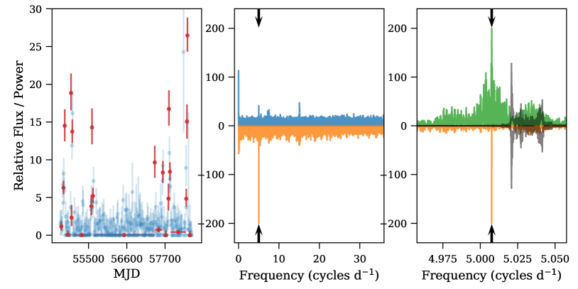
Figure 10: A modulation analysis of Cygnus X-3. (left) The 14-d light curve (blue, light points) and Bayesian blocks estimators (red, heavier points) for a piecewise-constant light curve. These light curves are used for photon reweighting. (middle) The power spectrum without (top, blue) and with (bottom, orange) reweighting. The arrows indicate the Cygnus X-3 orbital frequency. (right) A narrow band around the $f_{cyg}$, showing the re-weighted power spectrum without (top, green) and with (bottom, orange) spectral leakage reduction. The gray trace shows the Fermi window function shifted to 1/3 of its original frequency.

6 Reweighting

Finally, we consider the “reweighting” of photons. Such reweighting is appropriate when, e.g., one has obtained weights from a long period of time but wishes to analyze a short interval where the flux of the source of interest is substantially different to the mean, e.g. a flaring blazar. In this case, if $\alpha$ is the ratio of the source fluxes, then a new set of weights $w^{\prime}$ can be obtained from the original weights $w=s/(s+b)$:

$$w^{\prime}=\frac{\alpha\,s}{\alpha\,s+b}=\frac{\alpha\frac{s}{s+b}}{\alpha\frac{s}{s+b}+\frac{b}{s+b}}=\frac{\alpha\,w}{\alpha\,w+(1-w)},$$ (9)

and likewise the total expected source counts should be scaled by $\alpha$.

The adoption of reweighting solves a lingering problem in the application of photon weights to the search for binaries, namely that the use of photon weights worked poorly for sources with long-term variability. Briefly, the exposure-weighting technique of Corbet et al. (2007) uses the mean photon rate to scale the exposure correctly, so it adapts naturally to higher source rates. On the other hand, the use of a fixed set of weights effectively deweighted source photons during high-flux states. Here, we show how reweighting naturally accounts for slow source variability and gives optimal sensitivity for modulation searches.

For our example we take the microquasar Cygnus X-3. The detection of $\gamma$-ray modulation at its orbital frequency ($f_{cyg}=5.0076692$ d^-1 at MJD 56561, Bhargava et al., 2017) during radio and $\gamma$-ray flares was an important early result from the LAT (Abdo et al., 2009b) and a particular technical challenge given that $f_{cyg}$$\approx$$f_{sc}/3$, raising questions of systematic error. Distinguishing the two frequencies requires a long data span to provide good resolution in the power spectrum; on the other hand, Cygnus X-3 flares last typically only a few weeks. In previous LAT catalogs, Cygnus X-3 was too faint (and too soft) to be detected in time-averaged analysis, and it is only with the long data span and new capabilities of the Pass 8 event reconstruction that it is firmly detected in 8-year source lists.

To obtain a long, optimal power spectrum we have combined the methods of §4 and §5. First, we divided the data into 14-day cells and ran the BB algorithm to obtain a piecewise constant estimator for $\alpha(t)$ on long timescales. This time series appears in the left panel of Figure 10. We subsequently applied Eq. 9 using the appropriate value of $\alpha$ within each partition, taking care to also scale the total expected source counts (“S”). Finally, we compute the power spectrum using Eq. 6. In the middle panel, we show the power spectrum without reweighting (using the time-averaged weights) with the upper blue trace and that with reweighting (and spectral leakage reduction) with the lower orange trace. The reweighting increases the S/N by a factor of about 5, and also reduces artefacts by absorbing the low-frequency variation into the scale factor. In the rightmost panel, we show a narrow band around $f_{cyg}$. Here, the top trace shows the reweighted signal without spectral leakage reduction, while the bottom orange trace results from removing the signal at $f_{cyg}$ in the time domain and restoring it. The reweighting decreases the uniformity of the window function and broadens the range over which spectral power is leaked, making time-domain subtraction particularly effective. Finally, we show the window function shifted to from $f_{sc}$ to $f_{sc}/3$ to demonstrate how close $f_{cyg}$ is to $f_{sc}/3$ but also that they are clearly resolved. This is the strongest (and cleanest) $\gamma$-ray detection of the orbital modulation of Cygnus X-3 to date.

7 Discussion and Summary

We have introduced a method of retrospective analysis that approximates the full likelihood of Fermi-LAT data. Because of its speed and simplicity, it is suitable for a wide range of applications. In particular, monitoring large numbers of sources (e.g. AGN) can be done cheaply and with more sensitivity than simple aperture photometry. The methods are also well suited for probing the shortest variability timescales, and we demonstrated that an “omnibus” test for variability can be achieved by using short-in-time data cells along with the Bayesian blocks algorithm. We conclude the paper by considering a few additional applications.

To study faint pulsar wind nebula or supernova remnants, it is often useful to “gate” out emission from bright pulsars by selecting data only from the off-pulse (e.g. Grondin et al., 2013; Li et al., 2018). Rather than hard cuts, analysts can apply Eq. 9 to time-averaged weights derived for the pulsar using for $\alpha(t)$ the pulse profile. Thus, photons from the pulse peaks have a weight very close to 1, while those from the off-pulse will be given a weight close to 0. By taking the inverse of these weights, a data set retaining as much information as possible, but with the pulsar signal optimally diminished, is obtained.

In addition to the longer-period $\gamma$-ray binaries discussed in §5, a second class of sources emitting orbitally-modulated $\gamma$-rays are eclipsing millisecond pulsars in tight binaries, including the so-called black widows and red backs. In these systems, the pulsar wind can interact with the wind of either a compact, main sequence, or evolved companion, with the shocked interface emitting X-rays (e.g. Gentile et al., 2014) and $\gamma$-rays (e.g. An et al., 2017). As with the massive star binaries, changing the viewing angle with respect to the bulk flow of the wind produces a modulation in spectrum and intensity. Additionally, dense material ablated from the stellar surface can eclipse radio emission from the pulsar, and for nearly edge-on systems a direct eclipse of $\gamma$ rays can occur. Although rare, detection of such an eclipse would immediately identify the orbital period and constrain the system’s inclination. Romani et al. (2012) performed such a search using a photon-weighted based likelihood and a template of a complete eclipse to identify very marginal evidence for an eclipse of PSR J2215$+$5135. The methods here are sufficiently fast to enable a search of all Fermi LAT sources for such eclipses.

In this paper, we concentrated on characterizing variability or in discovering variability in known sources. However, a clear extension is the search for new variable sources, specifically those that are too faint to detect in time-averaged analyses but are strongly detected via flares. (Cygnus X-3 is a good example, as are many AGN.) In order to find new sources, it suffices simply to introduce a source over a series of test positions and compute a set of weights for each one. Provided the source is assigned a flux near threshold (so as not to perturb the background weights), the methods outlined here will work well, and e.g. the detection of variability with Bayesian blocks can motivate a dedicated followup with a full likelihood analysis.

Finally, we consider the applicability of the methods presented here to other wavebands and instruments. Although photon counting instruments are available from the THz through UV, and such data perfectably amenable to photon-weight analysis, the event rates are too high to be practical. On the other hand, imaging X-ray instruments, particularly those that have traded angular resolution for effective area, e.g. XMM-Newton, NICER, and the future Athena mission, are well suited. Indeed, the large collecting area and very good spectral resolution of Athena make fitting spectro-variability models with photon weights a very promising application. At still higher energies, coded aperture telescopes used for hard X-ray observations have intrinsically high backgrounds, and could benefit from weighted analyses. Finally, in order to characterize TeV sources, Cherenkov imaging telescopes must separate particle showers produced by $\gamma$ rays and cosmic rays. Residual cosmic ray events form a natural background and weights can be incorporated in two ways: (1) with a probabilistic classification based on properties of the shower (2) with astrophysical weighting based on the distribution of position and energies of events in an ROI, as done here.

In summary, we believe the methods introduced here hold great promise for more sophisticated LAT analyses and for application to a number of high-energy instruments both in operation and yet to come.

References

- Abdo et al. (2009a) Abdo, A. A., Ackermann, M., Ajello, M., et al. 2009a, ApJ, 706, L56, doi: 10.1088/0004-637X/706/1/L56
- Abdo et al. (2009b) —. 2009b, Science, 326, 1512, doi: 10.1126/science.1182174
- Abdo et al. (2010) —. 2010, ApJ, 720, 272, doi: 10.1088/0004-637X/720/1/272
- Abdo et al. (2011a) —. 2011a, ApJ, 733, L26, doi: 10.1088/2041-8205/733/2/L26
- Abdo et al. (2011b) —. 2011b, Science, 331, 739, doi: 10.1126/science.1199705
- Abdo et al. (2013) Abdo, A. A., Ajello, M., Allafort, A., et al. 2013, ApJS, 208, 17, doi: 10.1088/0067-0049/208/2/17
- Ackermann et al. (2012) Ackermann, M., Ajello, M., Ballet, J., et al. 2012, Science, 335, 189, doi: 10.1126/science.1213974
- Ackermann et al. (2016) Ackermann, M., Anantua, R., Asano, K., et al. 2016, ApJ, 824, L20, doi: 10.3847/2041-8205/824/2/L20
- Ackermann et al. (2017) Ackermann, M., Allafort, A., Baldini, L., et al. 2017, ApJ, 835, 219, doi: 10.3847/1538-4357/835/2/219
- Ajello & et al. (2019) Ajello, M., & et al. 2019, ApJS, in press
- An et al. (2017) An, H., Romani, R. W., Johnson, T., Kerr, M., & Clark, C. J. 2017, ApJ, 850, 100, doi: 10.3847/1538-4357/aa947f
- Atwood et al. (2013) Atwood, W., Albert, A., Baldini, L., et al. 2013, arXiv e-prints, arXiv:1303.3514. https://arxiv.org/abs/1303.3514
- Atwood et al. (2009) Atwood, W. B., Abdo, A. A., Ackermann, M., et al. 2009, ApJ, 697, 1071, doi: 10.1088/0004-637X/697/2/1071
- Bhargava et al. (2017) Bhargava, Y., Rao, A. R., Singh, K. P., et al. 2017, ApJ, 849, 141, doi: 10.3847/1538-4357/aa8ea4
- Bickel et al. (2008) Bickel, P., Kleijn, B., & Rice, J. 2008, ApJ, 685, 384, doi: 10.1086/590399
- Bruel (2019) Bruel, P. 2019, A&A, 622, A108, doi: 10.1051/0004-6361/201834555
- Buehler et al. (2012) Buehler, R., Scargle, J. D., Blandford, R. D., et al. 2012, ApJ, 749, 26, doi: 10.1088/0004-637X/749/1/26
- Caliandro et al. (2013) Caliandro, G. A., Hill, A. B., Torres, D. F., et al. 2013, MNRAS, 436, 740, doi: 10.1093/mnras/stt1615
- Corbet & Kerr (2010) Corbet, R. H. D., & Kerr, M. 2010, arXiv e-prints, arXiv:1001.4718. https://arxiv.org/abs/1001.4718
- Corbet et al. (2007) Corbet, R. H. D., Markwardt, C. B., & Tueller, J. 2007, ApJ, 655, 458, doi: 10.1086/509319
- Corbet et al. (2016) Corbet, R. H. D., Chomiuk, L., Coe, M. J., et al. 2016, ApJ, 829, 105, doi: 10.3847/0004-637X/829/2/105
- Dubus (2013) Dubus, G. 2013, A&A Rev., 21, 64, doi: 10.1007/s00159-013-0064-5
- Gentile et al. (2014) Gentile, P. A., Roberts, M. S. E., McLaughlin, M. A., et al. 2014, ApJ, 783, 69, doi: 10.1088/0004-637X/783/2/69
- Grondin et al. (2013) Grondin, M. H., Romani, R. W., Lemoine-Goumard, M., et al. 2013, ApJ, 774, 110, doi: 10.1088/0004-637X/774/2/110
- Guillemot & Kerr (2019) Guillemot, L., & Kerr, M. 2019, A&A, in prep.
- Hu & Zidek (2002) Hu, F., & Zidek, J. V. 2002, The Canadian Journal of Statistics / La Revue Canadienne de Statistique, 30, 347
- Johnson et al. (2018) Johnson, T. J., Wood, K. S., Kerr, M., et al. 2018, ApJ, 863, 27, doi: 10.3847/1538-4357/aad185
- Kerr (2010) Kerr, M. 2010, PhD thesis, University of Washington
- Kerr (2011) —. 2011, ApJ, 732, 38, doi: 10.1088/0004-637X/732/1/38
- Lande (2014) Lande, J. 2014, PhD thesis, Stanford University
- Leahy et al. (1983) Leahy, D. A., Darbro, W., Elsner, R. F., et al. 1983, ApJ, 266, 160, doi: 10.1086/160766
- Li et al. (2018) Li, J., Torres, D. F., Lin, T. T., et al. 2018, ApJ, 858, 84, doi: 10.3847/1538-4357/aabac9
- Lott et al. (2012) Lott, B., Escande, L., Larsson, S., & Ballet, J. 2012, A&A, 544, A6, doi: 10.1051/0004-6361/201218873
- Meyer et al. (2019) Meyer, M., Scargle, J. D., & Blandford, R. D. 2019, ApJ, 877, 39, doi: 10.3847/1538-4357/ab1651
- Ransom et al. (2011) Ransom, S. M., Ray, P. S., Camilo, F., et al. 2011, ApJ, 727, L16, doi: 10.1088/2041-8205/727/1/L16
- Romani et al. (2012) Romani, R. W., Filippenko, A. V., Silverman, J. M., et al. 2012, ApJ, 760, L36, doi: 10.1088/2041-8205/760/2/L36
- Scargle (1998) Scargle, J. D. 1998, ApJ, 504, 405, doi: 10.1086/306064
- Scargle et al. (2013) Scargle, J. D., Norris, J. P., Jackson, B., & Chiang, J. 2013, ApJ, 764, 167, doi: 10.1088/0004-637X/764/2/167
- Tanaka et al. (2011) Tanaka, Y. T., Stawarz, Ł., Thompson, D. J., et al. 2011, ApJ, 733, 19, doi: 10.1088/0004-637X/733/1/19
- The Fermi-LAT collaboration (2019) The Fermi-LAT collaboration. 2019, arXiv e-prints, arXiv:1902.10045. https://arxiv.org/abs/1902.10045
- Tompkins (1999) Tompkins, W. F. 1999, PhD thesis, STANFORD UNIVERSITY
- Wilson-Hodge et al. (2018) Wilson-Hodge, C. A., Malacaria, C., Jenke, P. A., et al. 2018, ApJ, 863, 9, doi: 10.3847/1538-4357/aace60