Synthesizing Action Sequences for Modifying Model Decisions

Abstract

When a model makes a consequential decision, e.g., denying someone a loan, it needs to additionally generate actionable, realistic feedback on what the person can do to favorably change the decision. We cast this problem through the lens of program synthesis, in which our goal is to synthesize an optimal (realistically cheapest or simplest) sequence of actions that if a person executes successfully can change their classification. We present a novel and general approach that combines search-based program synthesis and test-time adversarial attacks to construct action sequences over a domain-specific set of actions. We demonstrate the effectiveness of our approach on a number of deep neural networks.

1 Introduction

Today, predictive models are responsible for an ever-expanding spectrum of decisions, some of which are consequential to the lives and well-being of individuals—e.g., mortgage underwriting, job screening, healthcare decisions, criminal risk assessment, and many more. As such, questions about fairness and transparency have taken center stage in the debate over the increasing use of machine learning to automate decisions in sensitive domains, and a vibrant research community has emerged to explore and address the many facets of these questions.

In this paper, we are interested in the problem of providing actionable feedback to the subjects of algorithmic decision-making. For instance, imagine that you are denied a mortgage to buy your first home, thanks to a model that consumed a set of features and deemed you too risky. We envision that such an algorithmic process should additionally give you realistic, actionable feedback that will increase your chances of receiving a loan. For instance, you might receive the following feedback: increase your down payment by $1000 and limit credit card debt to a maximum of $5000 for the next two months. This is probably reasonable advice, in contrast with, say, a much harder to fulfill feedback like change your marital status from single to married.

We view this problem through the lens of program synthesis [1]: we want to synthesize an optimal sequence of instructions that a human can execute so that they favorably change the decision of some model. Optimality here is with respect to a measure of how hard it is for a person to perform the provided actions—we want to provide the simplest, cheapest feedback. There are many challenges in solving this problem: (i) the combinatorial blow-up in the space of action sequences, (ii) the fact that actions are parameterized by real values and have variable cost (e.g., increase savings by $X), (iii) and the fact that action ordering is important, e.g., you can only do A after you have done B or you can only do A if you are more than 35 years old.

To attack this problem, we make the key observation that the problem resembles that of generating adversarial examples [2, 3, 4, 5], where we usually want to slightly perturb the pixels of an input image to modify the classification, e.g., make a neural network think a dog is a panda. However, in our case, we are not looking for an imperceptible perturbation to the input features, but one that results from the application of real-world actions. With this view in mind, we present a new technique that adapts and combines (i) search-based program synthesis[6]to traverse the space of action sequences and (ii) optimization-based adversarial example generation[4]techniques to discover action parameters. This combination allows our approach to handle a rich class of (differentiable) models, e.g., deep neural networks, and complex domain-specific actions and cost models.

Setting and Consequences

At this point, it is important to recognize the possibility that the solution we propose for the problem setting may be vulnerable to unethical practices. Although our technique, in principle, may be used by users to maliciously game the system, we believe in its importance and cannot envision a world in which subjects are unable to understand and act on black-box decisions. One setting we envision is where users cannot adversarially attack the decision-maker as they do not have access to the model. The intention would be to use our technique as a means for the service provider to give meaningful and actionable feedback to its users, making the decision process more transparent.

Most Relevant Work

To our knowledge, the idea of providing actionable feedback for algorithmic decisions was first advocated by Wachter et al. [7] in a law article. Ustun et al. [8] implemented this idea by searching for a minimal change to input features to modify the classification of simple linear models (logistic regression). Their approach discretizes the feature space and encodes the search as an integer programming (IP) problem. Zhang et al. [9] consider a similar problem over neural networks composed of ReLUs, exploiting the linear structure of ReLUs to solve a series of LP problems to construct a convex region of positively classified points that are close to the input. Our work is different in a number of dimensions: (i) Our algorithm is quite general: by reducing the search to an optimization problem, à la test-time adversarial attacks, it can handle the general class of differentiable models (as well as differentiable action and cost definitions), instead of just linear models. (ii) We allow defining complex, nuanced actions that mimic real-world interventions, as opposed to arbitrary modifications to input features. (iii) Similarly, we allow encoding cost models to assign different costs to actions, with the goal of synthesizing the simplest feedback a person can act on. See Section 5 for an extended discussion of related work.

Contributions

Our contributions are:

• We define the problem of synthesizing optimal action sequences that can favorably change the output of a machine-learned model. We view the problem through the lens of program synthesis, where our goal is to synthesize a program over a domain-specific language of real-world actions specified by a domain expert.

• We present an algorithm that combines search-based program synthesis to traverse the space of action sequences and optimization-based test-time adversarial attacks to discover optimal parameters for action sequences. We demonstrate how to leverage the results of optimization to guide the combinatorial search.

• We implement our approach and apply it to a number of neural networks learned from popular datasets. Our results demonstrate the effectiveness of our approach, the benefits of our algorithmic decisions, and the robustness of the synthesized action sequences to noise.

2 Optimal Action Sequences

In this section, we formally define the problem of synthesizing optimal action sequences.

Decision-Making Model

We shall use $f:X\rightarrow\{0,1\}$ to denote a classifier over inputs in $X$. For simplicity of exposition, and without loss of generality, we restrict $f$ to be a binary classifier—our approach extends naturally to $k$-ary classifiers.

A DSL of Actions

For a given classification domain, we assume that we have a domain-specific set of actions $A=\{a_{1},\ldots,a_{n}\}$, perhaps curated by a domain expert. Each action $a\in A$ is a function $a:X\times R\rightarrow X$, where $R$ is the set of parameters that $a$ can take. For example, imagine $x\in X$ are features of a person applying for a loan. An action $a(x,1000)$ may be one that increases $x$’s savings by $\$1000$, resulting in $x^{\prime}\in X$.

For each action $a_{i}\in A$, we associate a cost function $c_{i}:X\times R\rightarrow\mathds{R}_{\geqslant 0}$, denoting the cost of applying $a_{i}$ on a given input and parameters. Making $c_{i}$ a function of inputs and parameters of an action allows us to define fine-grained cost functions, e.g., some actions may be easier for some people, but not for others. For instance, in the US, acquiring a credit card is much easier for someone with a credit history in contrast to someone who recently arrived on a work visa. Similarly, varying the parameter of an action should vary the cost, e.g., increase savings by $1000 should be much cheaper than increase savings by $1,000,000.

Additionally, for each action $a_{i}$, we associate a Boolean precondition $\mathit{pre}_{i}:X\times R\rightarrow\mathds{B}$, indicating whether action $a_{i}(x,r)$ is feasible for a given input $x$ and parameter $r$. There are a number of potential use cases for preconditions. For instance, the action of renting a car may be only allowed if you are over 21 years old; this can be encoded as the precondition $\emph{age}\geqslant 21$. Preconditions can also encode valid parameters, e.g., you cannot increase your credit score past 850, so an action which recommends increasing your credit score by $r$ will have the precondition $\emph{creditScore}+r\leqslant 850$.

Optimal Action Sequence

Fix an input $x\in X$ and assume that $f(x)=0$. Informally, our goal is to find the least-cost, feasible sequence of actions that can transform $x$ into an $x^{\prime}$ such that $f(x^{\prime})=1$.

Formally, we will define an action sequence using a pair of sequences $\langle\sigma,\rho\rangle$, denoting actions in $A$ and their corresponding parameters in $R$, respectively. Specifically, $\sigma$ is a sequence of integers in $[1,|A|]$ (action indices), and $\sigma_{i}$ denotes the $i$th element in this sequence. $\rho$ is a sequence of parameters such that each $\rho_{i}\in R$. We assume $|\rho|=|\sigma|=k$, and we will use $k$ throughout to denote $|\sigma|$.

Given pair $\langle\sigma,\rho\rangle$, in what follows, we will use $x_{i}=a_{\sigma_{i}}(x_{i-1},\rho_{i})$, where $i\in[1,k]$ and $x_{0}=x$. That is, variable $x_{i}$ refers to the result of applying the first $i$ actions defined by $\langle\sigma,\rho\rangle$ to the input $x$. We are therefore looking for a feasible, least-cost sequence of actions $a_{\sigma_{1}},\ldots,a_{\sigma_{k}}$ and associated parameters $\rho_{1},\ldots,\rho_{k}$, which, if applied starting at $x$, results in $x_{k}$ that is classified as 1 by $f$. This is captured by the following optimization problem:

$$\operatorname*{arg\,min}_{\langle\sigma,\rho\rangle} \sum_{i=1}^{k}c_{\sigma_{i}}(x_{i-1},\rho_{i})$$ (1)

subject to $$f(x_{k})=1\text{ and }\bigwedge_{i=1}^{k}\mathit{pre}_{\sigma_{i}}(x_{i-1},\rho_{i})$$

3 An Algorithm for Sequence Synthesis

Algorithm 1 Full synthesis algorithm

1:function synthesize(model $f$, instance $x$, actions $A$)

2:     $S\leftarrow\{\langle\sigma^{\emptyset},\rho^{\emptyset}\rangle\}$, where $\langle\sigma^{\emptyset},\rho^{\emptyset}\rangle$ are the empty action and parameters sequences, respectively

3:     repeat

4:         Let $\langle\sigma,\rho\rangle\in S$ and $a_{i}\in A$ be with smallest $\mathit{score}(\sigma,\rho,a_{i})$ $\triangleright$ $\langle\sigma a_{i},-\rangle\not\in S$

5:         Solve Problem 3 to compute parameters $\rho^{\prime}$ for sequence $\sigma a_{i}$

6:         $S\leftarrow S\cup\{\langle\sigma a_{i},\rho^{\prime}\rangle\}$

7:     until threshold exceeded $\triangleright$ threshold can be, e.g., search depth

8:     return Solution of Problem 1 restricted to sequences in $S$

We now present our technique for synthesizing action sequences, based on the optimization objective outlined above. Our algorithm assumes a differentiable model, e.g., a deep neural network, of the form $f:\mathds{R}^{m}\rightarrow\{0,1\}$, as well as differentiable actions, cost functions and preconditions. To solve Problem 1, defined in Section 2, we break it into two pieces: (i) a discrete search through the space of action sequences $\sigma$ and (ii) a continuous-optimization-based search through the space of action parameters $\rho$, which we assume to be real-valued.

In Section 3.1, we begin by describing the optimization technique, by assuming we have a fixed sequence of actions and setting up an optimization problem—an adaptation of Carlini and Wagner’s adversarial attack [4]—to learn the parameters to those actions. Then, in Section 3.2, we present the full algorithm, a search-based synthesis algorithm for discovering action sequences, which uses the optimization technique from Section 3.1 as a subroutine.

Remark on optimality: We note that the constrained optimization Problem 1 is hard in general—e.g., even very limited numerical planning problems that can be posed as Problem 1 are undecidable [10]. Our use of adversarial attacks in the following section necessarily relaxes some of the constraints and is therefore not guaranteed to result in optimal action sequences.

3.1 Adversarial Parameter Learning

We now assume that we have a fixed sequence of actions $\sigma$, as defined in Section 2. Our goal is to find the parameters $\rho$ such that $\langle\sigma,\rho\rangle$ satisfies the constraints of Problem 1. Specifically, our solution to this problem is an adaptation of Carlini and Wagner’s seminal adversarial attack technique against neural networks [4], but in a setting where the “attack” is comprised of a sequence of actions with preconditions and varying costs.

Henceforth, we shall assume that the model is a neural network $f:\mathds{R}^{m}\to\mathds{R}^{2}$ (where the output denotes a distribution over the two classification labels). Additionally, $f(x)=\text{softmax}(g(x))$, i.e., function $g$ is the output of the pre-softmax layers of the network.

Boolean Precondition Relaxation

Our goal is to construct a tractable optimization problem whose solution results in the parameters $\rho$ to the given action sequence $\sigma$. We begin by defining the following constrained optimization problem which relaxes the Boolean precondition constraints:

$$\operatorname*{arg\,min}_{\rho} ~{}\sum_{i=1}^{k}c_{\sigma_{i}}(x_{i-1},\rho_{i})+\mathit{pre}_{\sigma_{i}}^{\prime}(x_{i-1},\rho_{i})$$ (2)

subject to $$~{}f(x_{k})_{1}>f(x_{k})_{0}$$

where $f(x)_{j}$ is the probability of class $j$, and the function $\mathit{pre}_{i}^{\prime}$ is a continuous relaxation of the Boolean precondition $\mathit{pre}_{i}$. Specifically, we encode preconditions by imposing a high cost on violating them. For instance, if $\mathit{pre}_{i}(x,r)=x>c$, where $c$ is a constant, then we define $\mathit{pre}^{\prime}_{i}(x,r)=\tau\exp(-\tau^{\prime}(x-c))$, where $\tau$ and $\tau^{\prime}$ are hyperparameters. The hyperparameters $\tau$ and $\tau^{\prime}$ determine the steepness of the continuous boundaries; the values we choose are inversely proportional to the size of the domain of $x$. We detail our specific choices in the Appendix. Conjunctions of Boolean predicates are encoded as a summation of their relaxations. We can now define $C_{\sigma_{i}}(x_{i-1},\rho_{i})$ to be the overall cost incurred by the action-parameter pair $\langle\sigma_{i},\rho_{i}\rangle$, i.e.

$$C_{\sigma_{i}}(x_{i-1},\rho_{i})=c_{\sigma_{i}}(x_{i-1},\rho_{i})+\mathit{pre}_{\sigma_{i}}^{\prime}(x_{i-1},\rho_{i})$$

Carlini–Wagner Relaxation

Now that we have relaxed preconditions, what is left is the classification constraint $f(x_{k})_{1}>f(x_{k})_{0}$ in Problem 2. Following Carlini and Wagner, we transform the constraint $f(x_{k})_{1}>f(x_{k})_{0}$ into the objective function that is the distance between logit (pre-softmax) output: $h(x_{k})=max(0,g(x_{k})_{0}-g(x_{k})_{1})$.

This results in the following optimization problem:

$$\operatorname*{arg\,min}_{\rho}c\cdot h(x_{k})+\sum_{i=1}^{k}C_{\sigma_{i}}(x_{i-1},\rho_{i})$$ (3)

In practice, we perform an adaptive search for the best value of the hyperparameter $c$ as we solve the optimization problem: at a variable length interval $t$ of minimization steps, we determine how close the search is to the decision boundary and adjust $c$ and $t$ accordingly. The Appendix details the exact algorithm we use for updating $c$ and $t$.

Dataset/model	Network architecture	#Features	#Actions
German Credit Data	2 dense layers of 40 ReLUs	20	7
Adult Dataset	2 dense layers of 50 ReLUs	14	6
Fannie Mae Loan Perf.	5 dense layers of 200 ReLUs	21	5
Drawing Recognition	3 1D conv. layers, 1 dense layer of 1024 ReLUs	512 (pixels)	1

Table 1: Overview of datasets/models for evaluation; we will refer to a model by the italicized prefix of its name

3.2 Sequence Synthesis and Optimization

Now that we have defined the optimization problem for discovering parameters $\rho$ of a given action sequence $\sigma$, we proceed to describe the full algorithm, where we search the space of action sequences.

Algorithm Description

Algorithm 1 is a simple search guided by a parametric score function that directs the search—lower score is better. The algorithm maintains a set of sequences $S$, which initially is the pair $\langle\sigma^{\emptyset},\rho^{\emptyset}\rangle$, containing two empty sequences. In every iteration, the algorithm picks an action sequence in $S$, extends it with a new action from $A$, and solves optimization Problem 3 to compute a new set of parameters. The search process continues until some preset threshold is exceeded, e.g., we have covered all sequences of some length or we have discovered a sequence that is below some cost upper bound. Finally, we can return the best pair in $S$, i.e., the one with the minimal cost that changes the classification and satisfies all preconditions, as per Problem 1.

Defining the Scoring Function

The definition of the scoring function $\mathit{score}$ dictates the speed with which the algorithm arrives at an best action sequence. In our evaluation, we consider a number of definitions, the first of which, the vanilla definition, is simple, but often inefficient:

$$\mathit{score}_{v}(\sigma,\rho,a_{i})=k+1$$

This definition turns the search into a breadth-first search, as shorter sequences are evaluated first.

A more informed score function we consider is to simply return the value of the objective function in Problem 3 for a given sequence $\langle\sigma,\rho\rangle$. We call this function $\mathit{score}_{o}$. Notice that $\mathit{score}_{o}$ does not consider the action to apply, so the action with which to expand the sequence is chosen arbitrarily.

Next, we consider a more sophisticated scoring function: we want to pick the action that modifies the most important features. To do so, we use the gradient of model features, with respect to the target loss, as a proxy for the most important features. The idea is that we want to pick the action that modifies the features with the largest gradient. For every action $a_{i}\in A$, we use the $\emph{fp}(a_{i})$ to denote its footprint: the set of indices of the input features it can modify, e.g., $\emph{fp}(a_{i})=\{1,2\}$ means that it modifies features 1 and 2 and leaves all others unchanged. Given $\langle\sigma,\rho\rangle\in S$, let $x^{\prime}$ be the result of applying $\langle\sigma,\rho\rangle$ to the input instance $x$. We now define the score function as:

$$\mathit{score}_{g}(\sigma,\rho,a_{i})=-\operatorname*{mean}_{j\in\emph{fp}(a_{i})}\left|\frac{d\ell(f(x^{\prime}))}{dx_{j}}\right|$$

In other words, the score of applying $a_{i}$ after the sequence $\sigma$ depends on the average gradient of the target loss $\ell$—binary cross-entropy loss with respect to the target label, i.e., 1—with respect to the features in $a_{i}$’s footprint.

4 Implementation and Evaluation

Implementation

Our algorithm is implemented in Python 3, using TensorFlow [11]. Actions, along with their costs and preconditions, are implemented as instances of an Action Python class. The Adam Optimizer [12] is used to solve optimization Problem 3. For fast experimentation, we implemented a brute-force version of Algorithm 1 where all sequences up to some length $n$ are optimized in parallel using AWS Lambda—i.e., each sequence is optimized as a separate Lambda.

Research Questions

We have designed our experiments to answer the following research questions: Q1: Can our technique synthesize action sequences for non-trivial models and actions? Q2: How do different score functions impact algorithm performance? Q3: How robust are the synthesized action sequences to noise? Further, Q4: we explore other applications of our technique, beyond consequential decisions.

Domains for Evaluation

For exploring questions Q1-3, we consider three popular datasets: The German Credit Data [13] and the Fannie Mae Single Family Loan Performance [14] datasets have to do with evaluating loan applications—high or low risk. The Adult Dataset [13] predicts income as high or low—the envisioned use case is it can be used to set salaries. Table 1 summarizes our datasets and models: For each of the three datasets, we (i) trained a deep neural network for classification (in the case of the Fannie Mae dataset, we used the neural network from [9]), (ii) constructed a number of realistic actions along with their associated costs and preconditions, and (iii) randomly chose 100 negatively classified instances (i.e., 300 instances overall) from the test sets to apply our algorithm to.

The actions constructed for each domain cover both numerical and categorical features; a number of actions for each domain modify multiple features—e.g., change the debt-to-income ratio, or get a degree (which takes time and therefore increases age). The Appendix details all the actions and describes our encoding of actions that modify categorical features.

To explore Q4, we also consider the Drawing Recognition task [9] based on Google’s Quick, Draw! dataset [15]. The goal is to extend a drawing, represented as a set of straight lines, so as it is classified as, e.g., a cat. Hence, we only build one action for this model: add line from point $(a,b)$ to $(a^{\prime},b^{\prime})$.

4.1 Results

We are now ready to discuss the results. Henceforth, when we refer to optimal solution, we mean the best solution we find after Algorithm 1 has explored all sequences of length less than an upper bound.

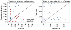
(a) Results for the German model

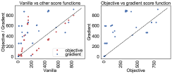
(b) Results for the Adult model

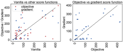
(c) Results for the Fannie Mae model

Figure 1: Number of optimization problems solved—i.e., loop iterations of Algorithm 1—before arriving at the optimal solution for different score functions. Each dot represents an instance.

Instances Solved

For our primary models, we make our algorithm consider all sequences of length $\leqslant 4$. The rationale behind this choice is that we usually want a small set of instructions to provide to an individual. Our algorithm was able to find solutions to 100/100 instances in the German model, 90/100 instances in the Adult model, and 62/100 instances in the Fannie Mae model. Note that inability to find a solution could be due to insufficient actions or incompleteness of the search—sequence length limit, relaxation of optimization problem, or local minima. In particular, the relatively inferior success rate on the Fannie Mae model may be a direct result of the fact that the neural network is much deeper.

To give an example of a synthesized action sequence by our algorithm, consider the following sequence of 3 actions for Fannie Mae: Increase credit score by 17 points, Reduce loan term by 43 months, and Increase interest rate by 0.621.

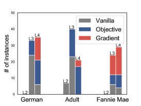
Figure 2: Performance of score functions as length of optimal sequence increases—L$x$ denotes optimal sequence of length $x$

Effects of Score Function

Next, we explore the effects of different score functions. Recall, in Section 3.2, we defined the vanilla score function $\mathit{score}_{v}$, where sequences are explored by length (a breadth-first search); the objective score function $\mathit{score}_{o}$, where the sequence with the smallest solution to Problem 3 is explored; and the gradient score function $\mathit{score}_{g}$, where gradient of cross-entropy loss is used to choose the sequence and action to explore.

Figure 1 shows the results of the German, Adult, and Fannie Mae models. Each point is one of the instances and the axes represent the iteration at which a score function arrived at the optimal sequence. The left plot compares $\mathit{score}_{v}$ vs $\mathit{score}_{g}$ (blue) and $\mathit{score}_{o}$ (red); the right plot compares $\mathit{score}_{o}$ vs $\mathit{score}_{g}$. We make two important observations: First, the vanilla score function excels on many instances (points above diagonal). After investigating those instances, we observe that they have short optimal sequences—of length 1 or 2. This is perhaps expected, as $\mathit{score}_{o}$ and $\mathit{score}_{g}$ may quickly lead the search towards longer sequences, missing short optimal ones until much later. We further illustrate this observation in Figure 2, where we plot the number of times each score function outperformed others (in terms of number of iterations of Algorithm 1) when the optimal solution is of length 2,3, and 4. We see that when optimal sequences are longer, $\mathit{score}_{v}$ stops being effective. Second, we observe that both the gradient and objective score functions, $\mathit{score}_{g}$ and $\mathit{score}_{o}$, have their merits, e.g., for Fannie Mae, $\mathit{score}_{g}$ dominates while for Adult $\mathit{score}_{o}$ dominates.

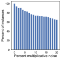
(a) German

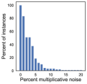
(b) Adult

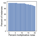
(c) Fannie Mae

Figure 3: Percent of instances ($y$-axis) that tolerate noise $\theta$ ($x$-axis) noise with probability $\geqslant 0.8$

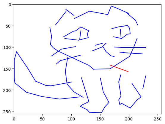
(a) sequence length = 1

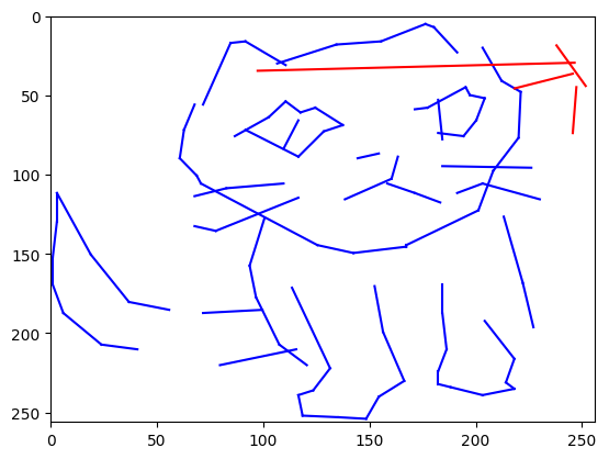
(b) sequence length = 4

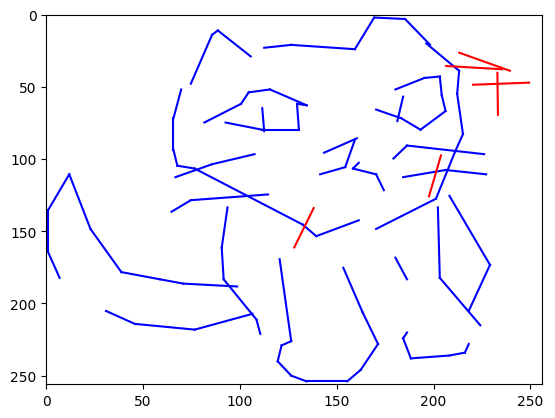
(c) sequence length = 6

Figure 4: Three different Quick, Draw! examples. Blue strokes comprise the input instance; red strokes are the results of applying actions.

Robustness of Synthesized Sequences

We now investigate how robust our solutions are to perturbations in their parameters. The idea is that a person given feedback from our algorithm may not be able to fulfil it precisely. We simulate this scenario by adding noise to the parameters of the optimal sequences. Specifically, for each synthesized optimal sequence and each parameter $r$ in the sequence, we uniformly sample values from the interval $[(1-\theta)r,(1+\theta)r]$, where $\theta$ is a parameter denoting the maximum percentage change.

Figure 3 summarizes the results for the three primary models. We plot the number of instances that succeed with a probability $\geqslant 0.8$ (i.e., are still solutions more than $80\%$ of the time) as the amount of noise $\theta$ increases. Obviously, when $\theta$ is 0, all instances succeed with probability 1; as $\theta$ increases, the success rate of a number of instances falls below $0.8$. We notice that the German and Fannie Mae solutions are quite robust, while only half of the Adult solutions can tolerate $\theta=0.03$ noise.

While our problem formulation does not enforce robustness of solutions, the results show that most instances are quite robust to noise. We attribute this phenomenon to the Carlini–Wagner relaxation. Recall that we minimize $\max(0,g(x_{k})_{0}-g(x_{k})_{1})$. So solutions need only get to a point where $g(x_{k})_{0}\leqslant g(x_{k})_{1}$—intuitively, barely beyond the decision boundary. However, we notice that, for most instances, solutions end up far from the boundary. Specifically, for the two models with more robust solutions, German and Fannie Mae, the average relative difference between $g_{1}$ and $g_{0}$—i.e., $(g(x_{k})_{1}-g(x_{k})_{0})/g(x_{k})_{1}$—is 3.41 (sd=6.79) and 1.92 (sd=5.40), respectively. For Adult, the average relative difference is much smaller, 0.09 (sd=0.06), indicating that most solutions where quite close to the decision boundary, explaining their sensitivity to noise.

It would be interesting to further improve robustness by incorporating it as a first-class constraint in our problem, e.g., by reformulating Problem 3 as a robust optimization [16] problem, so as we only discover solutions that are tolerant to noise. We plan to investigate this in future work.

Further Demonstration and Discussion

To further explore applications of our algorithm, we consider the Drawing Recognition model [9]. Each drawing in this model is composed of up to 128 straight line strokes. We considered 16 sketches of cats that are not classified as cats by this model. We constructed an action that adds a single line stroke, where the parameters to the action are the source and target $(x,y)$ coordinates. To ensure that the results of the actions are visible to the human eye, we add the precondition that stroke length is between 0.1 and 0.6 in length, where the image is $1\times 1$. The cost of an action is the length of the stroke.

We ran our algorithm up to and including length 6 ($\mathit{score}$ has no effect since there is a single action). Our algorithm managed to synthesize action sequences for 11/16 instances. Three representative solutions are shown in Figure 4. The first solution, of length 1, appears to be an additional whisker to the cat. The second and third solutions, lengths 4 and 6, appear to be more arbitrary and thus may be more adversarial in nature.

Note that our task is qualitatively different from [9]. They want to find the closest image across the decision boundary that has an $\epsilon$-ball around it. So they start with an adversarial example and incrementally expand it into a region of examples. Our problem is motivated by application of real-world actions, and therefore we search for a sequence of actions to modify an image.

The results of our technique on the Drawing Recognition model may seem to suggest that the solutions are adversarial in nature. However, it is hard to formally characterize the difference between an adversarial attack and a reasonable action sequence. In image-based attacks, it’s easy to tell if the modification is meaningful, but generally, e.g., in loans, this can probably be addressed by a domain-expert on a case-by-case basis. Observationally, we see that all our results look reasonable, i.e., there are no actions of the form modify X by $\epsilon$, where $\epsilon$ is very small for practical purposes. Moreover, our experiments show that most synthesized sequences are robust to random perturbations in their parameters, suggesting that they are not adversarial corner cases. One concrete way we can protect against generating adversarial feedback is to restrict our technique to models that are trained to be robust against adversarial attacks [17]—however, the definition of robustness will have to be tailored to the specific domain.

The seemingly unrealistic strokes produced as solutions in the Drawing Recognition model may stem from the fact that the cost function simply penalizes the length of the stroke and in no way drives the drawing of a ‘realistic’ stroke (In fact, it is not obvious how one can specify a cost function that encourages strokes which look realistic). The demonstration of our technique on this dataset serves to exhibit the versatility of our problem setting and proposed solution.

5 Related Work

We focus on works not discussed in Section 1.

Interpretable Machine Learning

Recently, there has been a huge interest in explainability in machine learning, particularly for deep neural networks. Most of the works have to do with highlighting the important features that led to a prediction, e.g., pixels of an image or words of a sentence. For instance, the seminal work on LIME [18] trains a simple local classifier and uses it to rank features by importance—many other works employ different techniques to hone in on important features, e.g.,  [19, 20, 21]. This is usually not enough: knowing, for instance, that your credit score affected the loan decision does not tell you how much you need to increase it by to be eligible for a loan, or whether there are other actions you can take. This is the distinguishing aspect of our work—providing actionable feedback.

Program Synthesis

We view our algorithm through the lens of program synthesis. Our algorithm is a form of enumerative program synthesis, a simple paradigm that has shown to be performant in many domains—see [6] for an overview. Our work is also related to differentiable programming languages [22, 23, 24, 25, 26]. The idea is to use numerical optimization to fill in the holes (parameters) in differentiable programs. Our work is similar in that we define a differentiable language of actions and costs and use numerical optimization to learn appropriate parameters for those actions. At an abstract level, our algorithm is similar in nature to that of [26]. They enumerate functional programs over neural networks and use optimization to learn parameters; here, we enumerate action sequences and use optimization to learn their parameters. There is also a growing body of work on using deep learning to perform and guide program synthesis, e.g.,  [27, 28, 29]

Symbolic synthesis techniques typically use SAT/SMT solvers to search the space of programs [30, 31]. Unfortunately, the range of programs they can encode is limited by decidable and practically efficient theories. While our problem can be encoded as an optimal SMT problem in linear arithmetic [32]—equivalently, an MILP problem—we will have to restrict all actions, costs, and models to be linear. In practice, this is quite restrictive. While our approach is incomplete, unlike in decidable first-order theories, it offers the flexibility and generality of being able to handle arbitrary differentiable models and actions.

Planning and Reinforcement Learning

Our problem can also be viewed as a planning problem in a continuous (or hybrid) domain. Most such planners are restricted to linear domains that are favorable to an SMT or MILP encoding or restricted forms of non-linearity, e.g., [33, 34, 35]. Some such planners also combine search and a form of optimization, typically LP, e.g., [36, 37]. Recently, [38] presented a scalable approach by reducing the planning problem to optimization and solving it with TensorFlow. In their setting, they deal with simple domains, e.g., 1 action; they do not have a goal state (in our case changing classification of a neural network), just a reward maximization objective; and they do not incorporate preconditions. Further, they are interested in very long plans over some time horizon, while our focus on generating small, actionable plans.

Our problem is also related to reinforcement learning (RL) with continuous action spaces, e.g., [39]. The power of RL is its ability to construct a general policy that can lead to a goal state. Thus, given a model, it would be interesting to use RL to learn a single policy that we can then apply to any input to the model, in contrast with our approach that learns a specific sequence of actions for every input.

6 Conclusion

We described a solution to the problem of presenting simple actionable feedback to subjects of a decision-making model so as to favorably change their classification. We presented a general solution where a domain expert specifies a differentiable set of actions that can be performed along with their costs. Then, we combine a search-based technique with an optimization technique to construct an optimal sequence of actions that leads to classification change. Our results demonstrate the promise of our technique and its applicability. There are many potential avenues for future work, e.g., exploring effects of different relaxations on optimality and robustness of results and adapting the algorithm to a complete black-box setting where we can only query the model. Another interesting avenue is to explore how our approach can be used to game the system in a strategic classification setting [40].

References

- [1] Sumit Gulwani, Oleksandr Polozov, and Rishabh Singh. Program synthesis. Foundations and Trends® in Programming Languages, (1-2):1–119, 2017.
- [2] Christian Szegedy, Wojciech Zaremba, Ilya Sutskever, Joan Bruna, Dumitru Erhan, Ian Goodfellow, and Rob Fergus. Intriguing properties of neural networks. arXiv preprint arXiv:1312.6199, 2013.
- [3] Ian J. Goodfellow, Jonathon Shlens, and Christian Szegedy. Explaining and harnessing adversarial examples. In ICLR, 2015.
- [4] Nicholas Carlini and David Wagner. Towards evaluating the robustness of neural networks. In S&P, 2017.
- [5] Nicolas Papernot, Patrick McDaniel, Ian Goodfellow, Somesh Jha, Z Berkay Celik, and Ananthram Swami. Practical black-box attacks against machine learning. In ACCS, 2017.
- [6] Rajeev Alur, Rishabh Singh, Dana Fisman, and Armando Solar-Lezama. Search-based program synthesis. CACM, (12), 2018.
- [7] Sandra Wachter, Brent Mittelstadt, and Chris Russell. Counterfactual explanations without opening the black box: Automated decisions and the GDPR. Harvard Journal of Law & Technology, (2), 2017.
- [8] Berk Ustun, Alexander Spangher, and Yang Liu. Actionable recourse in linear classification. In FAT*, 2019.
- [9] Xin Zhang, Armando Solar-Lezama, and Rishabh Singh. Interpreting neural network judgments via minimal, stable, and symbolic corrections. In NeurIPS, 2018.
- [10] Malte Helmert. Decidability and undecidability results for planning with numerical state variables. In AIPS, 2002.
- [11] Martín Abadi, Paul Barham, Jianmin Chen, Zhifeng Chen, Andy Davis, Jeffrey Dean, Matthieu Devin, Sanjay Ghemawat, Geoffrey Irving, Michael Isard, et al. Tensorflow: A system for large-scale machine learning. In OSDI, 2016.
- [12] Diederik P Kingma and Jimmy Ba. Adam: A method for stochastic optimization. arXiv preprint arXiv:1412.6980, 2014.
- [13] Dheeru Dua and Casey Graff. UCI machine learning repository, 2017.
- [14] Fannie Mae. Fannie Mae single-family loan performance data, 2014.
- [15] Google. The quick, draw! dataset.
- [16] Aharon Ben-Tal, Laurent El Ghaoui, and Arkadi Nemirovski. Robust optimization, volume 28. Princeton University Press, 2009.
- [17] Aleksander Madry, Aleksandar Makelov, Ludwig Schmidt, Dimitris Tsipras, and Adrian Vladu. Towards deep learning models resistant to adversarial attacks. In ICLR, 2018.
- [18] Marco Tulio Ribeiro, Sameer Singh, and Carlos Guestrin. Why should i trust you?: Explaining the predictions of any classifier. In KDD, 2016.
- [19] Anupam Datta, Shayak Sen, and Yair Zick. Algorithmic transparency via quantitative input influence: Theory and experiments with learning systems. In S&P, 2016.
- [20] Mukund Sundararajan, Ankur Taly, and Qiqi Yan. Axiomatic attribution for deep networks. In ICML, 2017.
- [21] Scott M Lundberg and Su-In Lee. A unified approach to interpreting model predictions. In NeurIPS, 2017.
- [22] Scott Reed and Nando De Freitas. Neural programmer-interpreters. arXiv preprint arXiv:1511.06279, 2015.
- [23] Matko Bošnjak, Tim Rocktäschel, Jason Naradowsky, and Sebastian Riedel. Programming with a differentiable forth interpreter. In ICML, 2017.
- [24] Alexander L. Gaunt, Marc Brockschmidt, Nate Kushman, and Daniel Tarlow. Differentiable programs with neural libraries. In ICML, 2017.
- [25] Alexander L Gaunt, Marc Brockschmidt, Rishabh Singh, Nate Kushman, Pushmeet Kohli, Jonathan Taylor, and Daniel Tarlow. Terpret: A probabilistic programming language for program induction. arXiv preprint arXiv:1608.04428, 2016.
- [26] Lazar Valkov, Dipak Chaudhari, Akash Srivastava, Charles Sutton, and Swarat Chaudhuri. Houdini: Lifelong learning as program synthesis. In NeurIPS, 2018.
- [27] Emilio Parisotto, Abdel-rahman Mohamed, Rishabh Singh, Lihong Li, Dengyong Zhou, and Pushmeet Kohli. Neuro-symbolic program synthesis. 2017.
- [28] Xinyun Chen, Chang Liu, and Dawn Song. Execution-guided neural program synthesis. In ICLR, 2019.
- [29] Rudy Bunel, Matthew Hausknecht, Jacob Devlin, Rishabh Singh, and Pushmeet Kohli. Leveraging grammar and reinforcement learning for neural program synthesis. In ICLR, 2018.
- [30] Armando Solar-Lezama, Liviu Tancau, Rastislav Bodik, Sanjit Seshia, and Vijay Saraswat. Combinatorial sketching for finite programs. ACM Sigplan Notices, (11), 2006.
- [31] Sumit Gulwani, Susmit Jha, Ashish Tiwari, and Ramarathnam Venkatesan. Synthesis of loop-free programs. In PLDI, 2011.
- [32] Yi Li, Aws Albarghouthi, Zachary Kincaid, Arie Gurfinkel, and Marsha Chechik. Symbolic optimization with smt solvers. In ACM SIGPLAN Notices, number 1, 2014.
- [33] Michael Cashmore, Maria Fox, Derek Long, and Daniele Magazzeni. A compilation of the full PDDL+ language into SMT. In Workshops at AAAI, 2016.
- [34] Wiktor Mateusz Piotrowski, Maria Fox, Derek Long, Daniele Magazzeni, and Fabio Mercorio. Heuristic planning for hybrid systems. In Thirtieth AAAI Conference on Artificial Intelligence, 2016.
- [35] Daniel Bryce, Sicun Gao, David Musliner, and Robert Goldman. SMT-based nonlinear PDDL+ planning. In Workshops at the Twenty-Ninth AAAI Conference on Artificial Intelligence, 2015.
- [36] Enrique Fernández-González, Brian Williams, and Erez Karpas. Scottyactivity: mixed discrete-continuous planning with convex optimization. JAIR, 62:579–664, 2018.
- [37] Amanda Jane Coles, Andrew I Coles, Maria Fox, and Derek Long. Colin: Planning with continuous linear numeric change. JAIR, 44:1–96, 2012.
- [38] Ga Wu, Buser Say, and Scott Sanner. Scalable planning with tensorflow for hybrid nonlinear domains. In NeurIPS, 2017.
- [39] Timothy P Lillicrap, Jonathan J Hunt, Alexander Pritzel, Nicolas Heess, Tom Erez, Yuval Tassa, David Silver, and Daan Wierstra. Continuous control with deep reinforcement learning. arXiv preprint arXiv:1509.02971, 2015.
- [40] Moritz Hardt, Nimrod Megiddo, Christos Papadimitriou, and Mary Wootters. Strategic classification. In ITCS, 2016.