Poirot: Aligning Attack Behavior with Kernel Audit Records for Cyber Threat Hunting

Abstract.

Cyber threat intelligence (CTI) is being used to search for indicators of attacks that might have compromised an enterprise network for a long time without being discovered. To have a more effective analysis, CTI open standards have incorporated descriptive relationships showing how the indicators or observables are related to each other. However, these relationships are either completely overlooked in information gathering or not used for threat hunting. In this paper, we propose a system, called Poirot, which uses these correlations to uncover the steps of a successful attack campaign. We use kernel audits as a reliable source that covers all causal relations and information flows among system entities and model threat hunting as an inexact graph pattern matching problem. Our technical approach is based on a novel similarity metric which assesses an alignment between a query graph constructed out of CTI correlations and a provenance graph constructed out of kernel audit log records. We evaluate Poirot on publicly released real-world incident reports as well as reports of an adversarial engagement designed by DARPA, including ten distinct attack campaigns against different OS platforms such as Linux, FreeBSD, and Windows. Our evaluation results show that Poirot is capable of searching inside graphs containing millions of nodes and pinpoint the attacks in a few minutes, and the results serve to illustrate that CTI correlations could be used as robust and reliable artifacts for threat hunting.

Preprint. The final version of this paper is going to appear in the ACM SIGSAC Conference on Computer and Communications Security (CCS’19), November 11-15, 2019, London, United Kingdom.

1. Introduction

When Indicators of Compromise (IOCs) related to an advanced persistent threat (APT) detected inside an organization are released, a common question that emerges among enterprise security analysts is if their enterprise has been the target of that APT. This process is commonly known as Threat Hunting. Answering this question with a high level of confidence often requires lengthy and complicated searches and analysis over host and network logs of the enterprise, recognizing entities that appear in the IOC descriptions among those logs and finally assessing the likelihood that the specific APT successfully infiltrated the enterprise.

In general, threat hunting inside an enterprise presents several challenges:

• Search at scale: To remain under the radar, an attacker often performs the attack steps over long periods (weeks, or in some cases, months). Hence, it is necessary to design an approach that can link related IOCs together even if they are conducted over a long period of time. To this end, the system should be capable of searching among millions of log events (99.9% of which often correspond to benign activities).

• Robust identification and linking of threat-relevant entities: Threat hunting must be sound in identifying whether an attack campaign has affected a system, even though the attacker might have mutated the artifacts like file hashes and IP addresses to evade detection. Therefore, a robust approach should not merely look for matching IOCs in isolation, but uncover the entire threat scenario, which is harder for an attacker to mutate.

• Efficient Matching: For a cyber analyst to understand and react to a threat incident in a timely fashion, the approach must efficiently conduct the search and not produce many false positives so that appropriate cyber-response operations can be initiated in a timely fashion.

Commonly, knowledge about the malware employed in APT campaigns is published in cyber threat intelligence (CTI) reports and is presented in a variety of forms such as natural language, structured, and semi-structured form. To facilitate the smooth exchange of CTI in the form of IOCs and enable characterization of adversarial techniques, tactics, and procedures (TTPs), the security community has adopted open standards such as OpenIOC (FireEye, 2018a), STIX (Mitre, 2018), and MISP (MISP, 2019). To provide a better overview of attacks, these standards often incorporate descriptive relationships showing how indicators or observables are related to each other (Iklody, 2019).

However, a vast majority of the current threat hunting approaches operates only over fragmented views of cyber threats(Systems, 2017; FireEye, 2018b), such as signatures (e.g., hashes of artifacts), suspicious file/process names, and IP addresses (domain names), or by using heuristics such as timestamps to correlate suspicious events (Pei et al., 2016). These approaches are useful but have limitations, such as (i) lacking the precision to reveal the complete picture as to how the threat unfolded especially over long periods (weeks, or in some cases, months), (ii) being susceptible to false signals when adversaries use legitimate-looking names (like svchost in Windows) to make their attacks indistinguishable from benign system activities, and (iii) relying on low-level signatures, which makes them ineffective when attackers update or re-purpose  (Symantec, 2019; Times, 2019) their tools or change their signatures (IP addresses or hash values) to evade detection. To overcome these limitations and build a robust detection system, the correlation among IOCs must be taken into account. In fact, the relationships between IOC artifacts contain essential clues on the behavior of the attacks inside a compromised system, which is tied to attacker goals and is, therefore, more difficult to change (Kolbitsch et al., 2009; Zong et al., 2015).

This paper formalizes the threat hunting problem from CTI reports and IOC descriptions, develops a rigorous approach for deriving the confidence score that indicates the likelihood of success of an attack campaign, and describes a system called Poirot that implements this approach. In a nutshell, given a graph-based representation of IOCs and relationships among them that expresses the overall behavior of an APT, which we call a query graph, our approach efficiently finds an embedding of this query graph in a much larger provenance graph, which contains a representation of kernel audit logs over a long period of time. Kernel audit logs are free of unauthorized tampering as long as system’s kernel is not compromised, and reliably contain relationships between system entities (e.g., processes, files, sockets, etc.), in contrast to its alternatives (e.g., firewall, network monitoring, and file access logs) which provide partial information. We assume that to maintain the integrity of kernel audit logs, a real-time kernel audit storage on a separate and secure log server is used as a precaution against log tampering.

More precisely, we formulate threat hunting as a graph pattern matching (GPM) problem searching for causal dependencies or information flows among system entities that are similar to those described in the query graph. To be robust against evasive attacks (e.g., mimicry attacks (Wagner and Soto, 2002; Parampalli et al., 2008)) which aim to influence the matching, we prioritize flows based on the cost they have for an attacker to produce. Given the NP-completeness of the graph matching problem (De Nardo et al., 2009), we propose an approximation function and a novel similarity metric to assess an alignment between the query and provenance graph.

We test Poirot’s effectiveness and efficiency using three different datasets, particularly, red-team/blue-team adversarial engagements performed by DARPA Transparent Computing (TC) program (Keromytis, 2018), publicly available real-world incident reports, and attack-free activities generated by ordinary users. In addition, we simulate several attacks from real-world scenarios in a controlled environment and compare Poirot with other tools that are currently used to do threat hunting. We show that Poirot outperforms these tools. We have implemented different kernel log parsers for Linux, FreeBSD, and Windows, and our evaluation results show that Poirot can search inside graphs containing millions of nodes and pinpoint the attacks in a few minutes.

This paper is organized as follows: Related work appears in  section 2. We present an overall architecture of Poirot in  section 3. In  section 4, we provide the formal details of the graph alignment algorithm.  Section 5 discusses the evaluation, and we conclude in  section 6.

2. Related Work

Log-based Attack Analytics. Opera et al. (Oprea et al., 2015) leverage DNS or web proxy logs for detecting early-stage infection in an enterprise. Disclosure (Bilge et al., 2012) extracts statistical features from NetFlow logs to detect botnet C&C channels. DNS logs have also been extensively used (Antonakakis et al., 2011, 2012) for detecting malicious domains. Hercule (Pei et al., 2016) uses community detection to reconstruct attack stages by correlating logs coming from multiple sources. Similar to Poirot, a large body of work uses system audit logs to perform forensic analysis and attack reconstruction(Goel et al., 2005b, a; Pohly et al., 2012; Liu et al., 2018).

Provenance Graph Explorations. The idea to construct a provenance graph from kernel audit logs was introduced by King et al. (King and Chen, 2003; King et al., 2005). The large size and coarse granularity of these graphs have limited their practical use. However, recent advancements have paved the way for more efficient and effective use of provenance graphs. Several approaches have introduced compression, summarization, and log reduction techniques (Lee et al., 2013b; Xu et al., 2016; Hossain et al., 2018) to differentiate worthy events from uninformative ones and consequently reduce the storage size. Dividing processes into smaller units is one of the approaches to add more granularity into the provenance graphs, and to this end, researchers have utilized different methods, such as dynamic binary analysis (Lee et al., 2013a; Ma et al., 2016), source code annotation (Ma et al., 2017), or modeling-based inference (Ma et al., 2015; Kwon et al., 2018; M. Milajerdi et al., 2018). Additionally, record-and-replay (Ji et al., 2017, 2018) and parallel execution methods (Kwon et al., 2016) are proposed for more precise tracking. Recent studies have leveraged provenance graphs for different objectives, such as alert triage (Hassan et al., 2019), zero-day attack path identification (Sun et al., 2018), attack detection and reconstruction (Milajerdi et al., 2019; Hossain et al., 2017). However, the scope of Poirot is different from these recent works, since it is focused on threat hunting and not real-time detection or forensic analysis.

Query Processing Systems. Prior works have incorporated novel optimization techniques, graph indexing, and query processing methods (Wang et al., 2012; Giugno and Shasha, 2002; Sun et al., 2012) to support timely attack investigations. SAQL (Gao et al., 2018a) is an anomaly query engine that queries specified anomalies to identify abnormal behaviors among system events. AIQL (Gao et al., 2018b) can be used as a forensic query system that has a domain-specific language for investigating attack campaigns from historical audit logs. Pasquier et al. (Pasquier et al., 2018) propose a query framework, called CamQuery, that supports real-time analysis on provenance graphs, to address problems such as data loss prevention, intrusion detection, and regulatory compliance. Shu et al. (Shu et al., 2018) also propose a human-assisted query system equipping threat hunters with a suite of potent new tools. These works are orthogonal to Poirot and can be used as a foundation to implement our search algorithm.

Behavior Discovery. Extracting malicious behaviors such as information flows and causal dependencies and searching for them as robust indicators have been investigated in prior works. Christodorescu et al. (Christodorescu et al., 2007) have proposed an approach for mining malware behavior from dynamic traces of that malware’s samples. Similarly, Kolbitsch et al. (Kolbitsch et al., 2009) automatically generate behavior models of malware using symbolic execution. They represent this behavior as a graph and search for it among the runtime behavior of unknown programs. On the contrary, Poirot does not rely on symbolic expressions but looks for correlations and information flows on the whole system. TGMiner (Zong et al., 2015) is a method to mine discriminative graph patterns from training audit logs and search for their existence in test data. The focus of this work is query formulation instead of pattern query processing, and the authors have used a subsequence matching solution (Zong et al., 2014) for their search, which is different from our graph pattern matching approach.

Graph Pattern Matching. Graph Pattern Matching (GPM) has proved useful in a variety of applications (Gallagher, 2006). GPM can be defined as a search problem inside a large graph for a subgraph containing similar connections conjunctively specified in a small query graph. This problem is NP-complete in the general case (De Nardo et al., 2009). Fan et. al. (Fan et al., 2010) proposed a polynomial time approach assuming that each connection in the pattern could only be mapped to a path with a predefined number of hops. Other works (Cheng et al., 2008; Zou et al., 2009) have tackled the problem by using a sequence of join functions in the vector space. NeMa (Khan et al., 2013) is a neighborhood-based subgraph matching technique based on the proximity of nodes. In contrast, G-Ray and later Mage(Tong et al., 2007; Pienta et al., 2014) take into account the shape of the query graph and edge attributes and are more similar to our approach, where similar information flows and causal dependencies play a crucial role. However, these approaches work based on random-walk, which is not reliable against attackers (with knowledge of the threat-hunting method) who generate fake events (as explained in section 4.1). While our graph alignment notions are similar to these works, the graph characteristics Poirot analyzes present new challenges such as being labeled, directed, typed, in the order of millions of nodes, and constructed in an adversarial setting. Moreover, many of these related works are looking for a subgraph that contains exactly one alignment for each node and each edge of the query graph and cannot operate in a setting where there might not be an alignment for certain nodes or edges. As a result, we develop a new best-effort matching technique aimed at tackling these challenges.

3. Approach Overview

A high-level view of our approach is shown in Figure 1. We provide a brief overview of the components of Poirot next, with more detailed discussions relegated to section 4.

3.1. Provenance Graph Construction

To determine if the actions of the APT appear in the system, we model the kernel audit logs as a labeled, typed, and directed graph, which we call provenance graph ($G_{p}$). This is a common representation of kernel audit logs, which allows tracking causality and information flow efficiently (King and Chen, 2003, 2005; Gao et al., 2018b; Gao et al., 2018a; Hossain et al., 2017). In this graph, nodes represent system entities involved in the kernel audit logs, which have different types such as files and processes, while edges represent information flow and causality among those nodes taking into account the direction. Poirot currently supports consuming kernel audit logs from Microsoft Windows, Linux, and FreeBSD and constructs a provenance graph in memory, similar to prior work in this area (Hossain et al., 2017). To support efficient searching on this graph, we leverage additional methods such as fast hashing techniques and reverse indexing for mapping process/file names to unique node IDs.

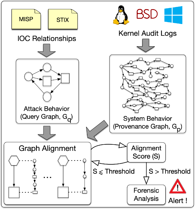
Figure 1. Poirot Approach Overview.

3.2. Query Graph Construction

We extract IOCs together with the relationships among them from CTI reports related to a known attack. These reports appear in security blogs, threat intelligence reports by industry, underground forums on cyber threats, and public and private threat intelligence feeds. In addition to natural language, the attacks are often described in structured and semi-structured standard formats as well. These formats include OpenIOC(FireEye, 2018a), STIX(Mitre, 2018), MISP(MISP, 2019), etc. Essentially, these exchange formats are used to describe the salient points of the attacks, the observed IOCs, and the relationships among them. For instance, using OpenIOC the behavior of a malware sample can be described as a list of artifacts such as the files it opens, and the DLLs it loads  (FireEye, 2013). These standard descriptions are usually created by the security operators manually (team, 2013a, b). Additionally, automated tools have also been built to automatically extract IOCs from natural language and complement the work of human operators (Zhu and Dumitras, 2018; Liao et al., 2016; Husari et al., 2017). These tools can be used to perform an initial extraction of features to generate the query graph and later refined manually by a security expert. We believe that manual refinement is an important component of the query graph construction because automated methods may often generate noise and reduce the quality of the query graphs.

We model the behavior appearing in CTI reports also as a labeled, typed, and directed graph, which we call query graph ($G_{q}$). If a description in a standard format is present, the creation of the query graph can be easily automated and further refined by humans. In particular, the entities appearing in the reports (e.g., processes, files) are transformed into nodes while relationships are transformed into directed edges (STIX, 2019). Nodes and edges of the query graph may be further associated with additional information such as labels (or names), types (e.g., processes, files, sockets, pipes, etc) and other annotations (e.g., hash values, creation time, etc) depending on the information that an analyst may deem necessary for matching. In the current Poirot implementation, we use names and types for specifying explicit mappings between nodes in the query graph and nodes in the provenance graph.

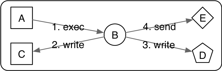
Figure 2. Query Graph of DeputyDog Malware. A=$*$.%exe%, B=$*$, C=%APPDATA%\$*$, D=%HKCU%\Software\Microsoft\Windows\CurrentVersion\ Run\$*$, E=%External  IP  address%.

As an example of query graph construction, consider the following excerpt from a report (Moran and Villeneuve, 2013) about the DeputyDog malware, used in our evaluation.
Upon execution, 8aba4b5184072f2a50cbc5ecfe326701 writes “28542CC0.dll” to this location: “C:\Documents and Settings\All Users\Application Data\28542CC0.dll”. In order to maintain persistence, the original malware adds this registry key: “%HKCU%\Software\Microsoft\Windows\CurrentVersion\Run\ 28542CC0”. The malware then connects to a host in South Korea (180.150.228.102).

The excerpt mentions several actions and entities that perform them and is readily transformed into a graph by a security analyst. For instance, the first sentence clearly denotes a process writing to a file (upon execution the malware writes a file to a location). We point out that the level of detail present in this excerpt is common across a large majority of CTI reports and can be converted to a reliable query graph by a qualified cyber analyst. In particular, the verbs that express actions carried out by subjects can often be easily mapped to reads/writes from/to disk or network and to interactions among processes (e.g., a browser downloads a file, a process spawns another process, a user clicks on a spear-phishing link, etc).

Figure 2 shows the query graph corresponding to the above excerpt. Ovals, diamonds, rectangles, and pentagons represent processes, sockets, files, and registry entries, respectively . In Figure 2, node B represents the malware process or group of processes (we use a $*$ to denote that it can have any name), node A represents the image file of the malware, while nodes C, D and E represent a dropped file, a registry and an Internet location, respectively. We highlight at this point that the query graph that is built contains only information about information flows among specific entities as they appear in the report (processes, files, IP addresses, etc) and is not intended to be a precise subgraph of all the malicious entities that actually appear during the attack. In a certain sense, the query graph is a summary of the actual attack graph. In our experiments, the query graphs we obtained were usually small, containing between 10-40 nodes and up to 150 edges.

3.3. Graph Alignment

Finally, we model threat hunting as determining whether the query graph $G_{q}$ for the attack “manifests” itself inside the provenance graph $G_{p}$. We call this problem Graph Alignment Problem.

We note at this point that $G_{q}$ expresses several high-level flows between the entities (processes to files, etc.). In contrast, $G_{p}$ expresses the complete low-level activity of the system. As a result, an edge in $G_{q}$ might correspond to a path in $G_{p}$ consisting of multiple edges. For instance, if $G_{q}$ represents a compromised browser writing to a system file, in $G_{p}$ this may correspond to a path where a node representing a Firefox process forks new processes, only one of which ultimately writes to the system file. Often, this kind of correspondence may be created by attackers adding noise to their activities to escape detection. Therefore, we need a graph alignment technique that can match single edges in $G_{q}$ to paths in $G_{p}$. This requirement is critical in the design of our algorithm.

In graph theory literature, there exist several versions of the graph matching problem. In exact matching, the subgraph embedded in a larger graph $G_{p}$ must be isomorphic to $G_{q}$ (Zong et al., 2014). In contrast, in the graph pattern matching (GPM) problem, some of the restrictions of exact matching are relaxed to extract more useful subgraphs. However, both problems are NP-complete in the general case (De Nardo et al., 2009). Even though a substantial body of work dedicated to GPM exists (Gallagher, 2006; Fan et al., 2010; Cheng et al., 2008; Zou et al., 2009; Khan et al., 2013; Tong et al., 2007; Pienta et al., 2014), many have limitations that make them impractical to be deployed in the field of threat hunting. Specifically, they (i) are not designed for directed graphs with labels and types assigned to each node, (ii) do not scale to millions of nodes, or (iii) are designed to align all nodes or edges in the query graph exhaustively. Moreover, these approaches are not intended for the context of threat hunting, taking into account an evasive adversary which tries to remain stealthy utilizing the knowledge of the underlying matching criteria. Due to these considerations, we devise a novel graph pattern matching technique that addresses these limitations.

In Figure 1, graph nodes are represented in different shapes to model different node types, such as a file, process, and socket, however, the labels are omitted for brevity. In particular, Poirot starts by finding the set of all possible candidate alignments $i:j$ where $i$ and $j$ represent nodes in $V(G_{q})$ and $V(G_{p})$, respectively. Then, starting from the alignment with the highest likelihood of finding a match, called a seed node, we expand the search to find further node alignments. The seed nodes are represented by hexagons in Figure 1 while matching nodes in the two graphs are connected by dotted lines. To find an alignment that corresponds to the attack represented in CTI relationships, the search is expanded along paths that are more likely to be under the influence of an attacker. To estimate this likelihood, we devise a novel metric named influence score. Using this metric allows us to largely exclude irrelevant paths from the search and efficiently mitigate the dependency explosion problem. Prior works have also proposed approaches to prioritize flows based on a score computed as length (Khan et al., 2013; Tong et al., 2007) or cost (Hossain et al., 2017). However, they can be defeated by attacks (Wagner and Soto, 2002; Parampalli et al., 2008) in which attackers frequently change their ways to evade the detection techniques. For instance, a proximity-based graph matching approach (Khan et al., 2013; Tong et al., 2007) might be easily evaded by attackers, who, being aware of the underlying system and matching approach, might generate a long chain of fork commands to affect the precision of proximity-based graph matching. In contrast, our score definition explicitly takes the influence of a potential attacker into account. In particular, we increase the cost for the attacker to evade our detection, by prioritizing flows based on the effort it takes for an attacker to produce them. Our search for alignment uses such prioritized flows and is described in section 4.

After finding an alignment $G_{q}::G_{p}$, a score is calculated, representing the similarity between $G_{q}$ and the aligned subgraph of $G_{p}$. When the score is higher than a threshold value, Poirot raises an alert which declares the occurrence of an attack and presents a report of aligned nodes to a system analyst for further forensic analysis. Otherwise, Poirot starts an alignment from the next seed node candidate. After finding an attack subgraph in $G_{p}$, Poirot generates a report containing the aligned nodes, information flows between them, and the corresponding timestamps. In an enterprise setting, such visually compact and semantic-rich reports provide actionable intelligence to cyber analysts to plan and execute cyber-threat responses. We discuss the details of our approach in section 4.

4. Algorithms

In this section, we discuss our main approach for alignment between $G_{q}$ and $G_{p}$ by (a) defining an alignment metric to measure how proper a graph alignment is, and (b) designing a best-effort similarity search based on specific domain characteristics.

4.1. Alignment Metric

Notation	Description
$i:k$	Node alignment. Node $i$ is aligned to node $k$ ($i$ and $k$ are in two distinct graphs).
$i\mathrel{\mathchoice{\mathrel{}\mathrel{\mathop{\dabar@\dabar@}\limits}\mathrel{\mathchar 0\relax\symAMSa 04B}{}}{\mathrel{}\mathrel{\mathop{\dabar@\dabar@}\limits}\mathrel{\mathchar 0\relax\symAMSa 04B}{}}{\mathrel{}\mathrel{\mathop{\dabar@\dabar@}\limits}\mathrel{\mathchar 0\relax\symAMSa 04B}{}}{\mathrel{}\mathrel{\mathop{\dabar@\dabar@}\limits}\mathrel{\mathchar 0\relax\symAMSa 04B}{}}}j$	Flow. A path starting at node $i$ and ending at node $j$.
$i\xrightarrow[]{\text{label}}j$	An edge from node $i$ to node $j$ with a specific label.
$G_{q}::G_{p}$	Graph alignment. A set of node alignments $i:k$ where $i$ is a node of $G_{q}$ and $k$ is a node of $G_{p}$.
$V(G)$	Set of all vertices in graph $G$.
$E(G)$	Set of all edges in graph $G$.
$F(G)$	Set of all flows $i\mathrel{\mathchoice{\mathrel{}\mathrel{\mathop{\dabar@\dabar@}\limits}\mathrel{\mathchar 0\relax\symAMSa 04B}{}}{\mathrel{}\mathrel{\mathop{\dabar@\dabar@}\limits}\mathrel{\mathchar 0\relax\symAMSa 04B}{}}{\mathrel{}\mathrel{\mathop{\dabar@\dabar@}\limits}\mathrel{\mathchar 0\relax\symAMSa 04B}{}}{\mathrel{}\mathrel{\mathop{\dabar@\dabar@}\limits}\mathrel{\mathchar 0\relax\symAMSa 04B}{}}}j$ in graph $G$ such that $i\neq j$.

Table 1. Notations.

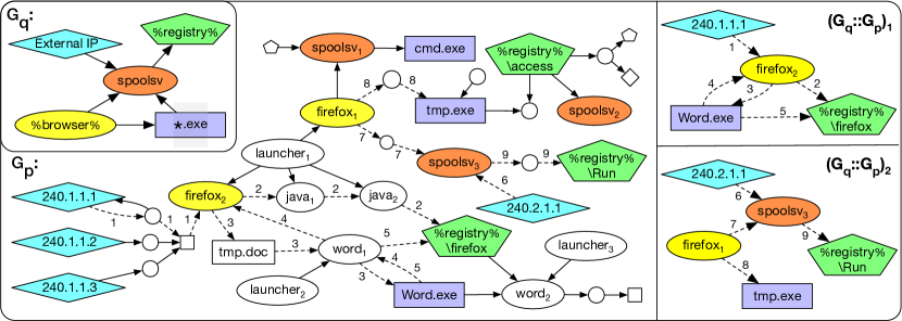
Figure 3. Simplified Provenance Graph ($G_{p}$), Query Graph ($G_{q}$), and two sample graph alignments ($G_{q}::G_{p}$). Node types are shown with different shapes, and possible alignments for each node is shown with the same color. The numbers on the edges are merely to illustrate possible paths/flows and do not have additional meaning.

We introduce some notations (in table 1), where we define two kinds of alignments, i.e., a node alignment between two nodes in two different graphs, and a graph alignment which is a set of node alignments. Typically, two nodes $i$ and $j$ are in a node alignment when they represent the same entity, e.g., a node representing a commonly used browser mentioned in the CTI report (node %browser% in the query graph $G_{q}$ of Figure 3) and a node representing a Firefox process in the provenance graph. We note that, in general, the node alignment relationship is a many-to-many relationship from V($G_{q}$) to V($G_{p}$), where V($G_{q}$) and V($G_{p}$) are the set of vertices of $G_{q}$ and $G_{p}$ respectively. Therefore, given a query graph $G_{q}$, there may be a large number of graph alignments between $G_{q}$ and many subgraphs of $G_{p}$. Another thing to point out is that each of these graph alignments can correspond to different subgraphs of $G_{p}$. Each of these subgraphs contains the nodes that are aligned with the nodes of $G_{q}$; however, they may contain different paths among those nodes. Among these subgraphs, we are interested in finding the subgraph that best matches the graph $G_{q}$.

Based on these definitions, the problem is to find the best possible graph alignment among a set of candidate graph alignments. To illustrate this problem, consider the query and provenance graphs $G_{q}$ and $G_{p}$, and two possible aligned graphs in Figure 3, where the node shapes represent entity types (e.g., process, file, socket), and the edges represent information flow (e.g., read, write, IPC) and causal dependencies (e.g., fork, clone) between nodes. The numbers shown on the edges of $G_{p}$ are not part of the provenance graph but serve to identify a single path in our discussion. In addition, the subgraphs of $G_{p}$ determined by these two graph alignments with $G_{q}$ are represented by dotted edges in $G_{p}$. Each flow in $G_{p}$ and corresponding edge in $G_{q}$ is labeled with the same number. The problem is, therefore, to decide which among many alignments is the best candidate. Intuitively, for this particular figure, alignment $(G_{q}::G_{p})_{2}$ is closer to $G_{q}$ than $(G_{q}::G_{p})_{1}$, mainly because the number of its aligned nodes is higher than that of $(G_{q}::G_{p})_{1}$, and most importantly, its flows have a better correspondence to the edges of the query graph $G_{q}$.

4.1.1. Influence Score

Before formalizing the intuition expressed above, we must introduce a path scoring function, which we call influence score and which assigns a number to a given flow between two nodes. This score will be instrumental in defining the “goodness” of a graph alignment. In practice, the influence score represents the likelihood that an attacker can produce a flow. To illustrate this notion, consider the two nodes firefox₂ and %registry%\firefox in the graph $G_{p}$ in Figure 3. There exist two flows from firefox₂ to %registry%\firefox, one represented by the edges labeled with the number 2 (and passing through nodes java₁ and java₂), and another represented by the edges labeled 3, 3, and 5 (and passing through nodes tmp.doc and word₁). Assuming firefox₂ is under the control of an attacker, it is more likely for the attacker to execute the first flow rather than the second flow. In fact, in order to exercise the second flow, an attacker would have to take control over process launcher₂ or word₁ in addition to firefox₂. Since launcher₂ or word₁ share no common ancestors in the process tree with firefox₂, such takeover would have to involve an additional exploit for launcher₂ or word₁, which is far more unlikely than simply exercising the first flow, where all processes share a common ancestor launcher₁. We point out that this likelihood does not depend on the length of the flow, rather on the number of processes in that flow and on the number of distinct ancestors those processes share in the process tree. One can, in fact, imagine a long chain of forked processes, which are however all under the control of the attacker because they all share a common ancestor in the process tree, i.e., the first process of the chain. Another possible scenario of attacks present in the wild involves remote code loading from a single compromised process, where all the code with malicious functionality is loaded in main memory and the same process (e.g., firefox) executes all the actions on behalf of the attacker. While this technique leaves no traces on the file system and may evade some detection tools, Poirot would be able to detect this kind of attack. In fact the influence score remains trivially unchanged.

One additional important point to note is that this notion of measuring the potential influence of an attacker is very robust concerning evasion methods from an attacker. Every activity that an attacker may use to add noise and try to evade detection will likely have the same common ancestors, namely the initial compromise points of the attack, unless the attacker pays a higher cost to perform more distinct compromises. Thus, such efforts will be ineffective in changing the influence score of the paths.

Based on these observations, we define the influence score, $\Gamma_{i,j}$, between a node $i$ and a node $j$ as follows:

(1) $$\Gamma_{i,j}=\begin{cases}\max\limits_{i\mathrel{\mathchoice{\mathrel{}\mathrel{\mathop{\dabar@\dabar@}\limits}\mathrel{\mathchar 0\relax\symAMSa 04B}{}}{\mathrel{}\mathrel{\mathop{\dabar@\dabar@}\limits}\mathrel{\mathchar 0\relax\symAMSa 04B}{}}{\mathrel{}\mathrel{\mathop{\dabar@\dabar@}\limits}\mathrel{\mathchar 0\relax\symAMSa 04B}{}}{\mathrel{}\mathrel{\mathop{\dabar@\dabar@}\limits}\mathrel{\mathchar 0\relax\symAMSa 04B}{}}}j}{\dfrac{1}{C_{min}(i\mathrel{\mathchoice{\mathrel{}\mathrel{\mathop{\dabar@\dabar@}\limits}\mathrel{\mathchar 0\relax\symAMSa 04B}{}}{\mathrel{}\mathrel{\mathop{\dabar@\dabar@}\limits}\mathrel{\mathchar 0\relax\symAMSa 04B}{}}{\mathrel{}\mathrel{\mathop{\dabar@\dabar@}\limits}\mathrel{\mathchar 0\relax\symAMSa 04B}{}}{\mathrel{}\mathrel{\mathop{\dabar@\dabar@}\limits}\mathrel{\mathchar 0\relax\symAMSa 04B}{}}}j)}}&\exists i\mathrel{\mathchoice{\mathrel{}\mathrel{\mathop{\dabar@\dabar@}\limits}\mathrel{\mathchar 0\relax\symAMSa 04B}{}}{\mathrel{}\mathrel{\mathop{\dabar@\dabar@}\limits}\mathrel{\mathchar 0\relax\symAMSa 04B}{}}{\mathrel{}\mathrel{\mathop{\dabar@\dabar@}\limits}\mathrel{\mathchar 0\relax\symAMSa 04B}{}}{\mathrel{}\mathrel{\mathop{\dabar@\dabar@}\limits}\mathrel{\mathchar 0\relax\symAMSa 04B}{}}}j\ |\ C_{min}(i\mathrel{\mathchoice{\mathrel{}\mathrel{\mathop{\dabar@\dabar@}\limits}\mathrel{\mathchar 0\relax\symAMSa 04B}{}}{\mathrel{}\mathrel{\mathop{\dabar@\dabar@}\limits}\mathrel{\mathchar 0\relax\symAMSa 04B}{}}{\mathrel{}\mathrel{\mathop{\dabar@\dabar@}\limits}\mathrel{\mathchar 0\relax\symAMSa 04B}{}}{\mathrel{}\mathrel{\mathop{\dabar@\dabar@}\limits}\mathrel{\mathchar 0\relax\symAMSa 04B}{}}}j)\leq C_{thr}\\ 0&\text{otherwise}\end{cases}$$

In Equation 1, $C_{min}(i\mathrel{\mathchoice{\mathrel{}\mathrel{\mathop{\dabar@\dabar@}\limits}\mathrel{\mathchar 0\relax\symAMSa 04B}{}}{\mathrel{}\mathrel{\mathop{\dabar@\dabar@}\limits}\mathrel{\mathchar 0\relax\symAMSa 04B}{}}{\mathrel{}\mathrel{\mathop{\dabar@\dabar@}\limits}\mathrel{\mathchar 0\relax\symAMSa 04B}{}}{\mathrel{}\mathrel{\mathop{\dabar@\dabar@}\limits}\mathrel{\mathchar 0\relax\symAMSa 04B}{}}}j)$ represents the minimum number of distinct, independent compromises an attacker has to conduct to be able to generate the flow $i\mathrel{\mathchoice{\mathrel{}\mathrel{\mathop{\dabar@\dabar@}\limits}\mathrel{\mathchar 0\relax\symAMSa 04B}{}}{\mathrel{}\mathrel{\mathop{\dabar@\dabar@}\limits}\mathrel{\mathchar 0\relax\symAMSa 04B}{}}{\mathrel{}\mathrel{\mathop{\dabar@\dabar@}\limits}\mathrel{\mathchar 0\relax\symAMSa 04B}{}}{\mathrel{}\mathrel{\mathop{\dabar@\dabar@}\limits}\mathrel{\mathchar 0\relax\symAMSa 04B}{}}}j$. This value captures the extent of the attacker’s control over the flow and is calculated based on the minimum number of common ancestors of the processes present in the flow. For instance, if there is a flow from a node $i$ to a node $j$, and all the processes involved in that flow have one common ancestor in the process tree, an attacker needs to compromise only that common ancestor process to initiate such flow, and therefore $C_{min}(i\mathrel{\mathchoice{\mathrel{}\mathrel{\mathop{\dabar@\dabar@}\limits}\mathrel{\mathchar 0\relax\symAMSa 04B}{}}{\mathrel{}\mathrel{\mathop{\dabar@\dabar@}\limits}\mathrel{\mathchar 0\relax\symAMSa 04B}{}}{\mathrel{}\mathrel{\mathop{\dabar@\dabar@}\limits}\mathrel{\mathchar 0\relax\symAMSa 04B}{}}{\mathrel{}\mathrel{\mathop{\dabar@\dabar@}\limits}\mathrel{\mathchar 0\relax\symAMSa 04B}{}}}j)$ is equal to 1. Note that if a node $i$ represents a process and node $j$ a child process of $i$, then $C_{min}(i\mathrel{\mathchoice{\mathrel{}\mathrel{\mathop{\dabar@\dabar@}\limits}\mathrel{\mathchar 0\relax\symAMSa 04B}{}}{\mathrel{}\mathrel{\mathop{\dabar@\dabar@}\limits}\mathrel{\mathchar 0\relax\symAMSa 04B}{}}{\mathrel{}\mathrel{\mathop{\dabar@\dabar@}\limits}\mathrel{\mathchar 0\relax\symAMSa 04B}{}}{\mathrel{}\mathrel{\mathop{\dabar@\dabar@}\limits}\mathrel{\mathchar 0\relax\symAMSa 04B}{}}}j)$ will be equal to 1 as $i$ is parent of $j$. If the number of common ancestors is larger than one (e.g., there are two ancestors in the path firefox₂ $\rightarrow tmp.doc\rightarrow word_{1}\rightarrow$ %registry%\firefox), an attacker has to compromise at least as many (unrelated) processes independently; therefore it is harder for the attacker to construct such flow. For instance, for the attacker to control the flow firefox₂ $\rightarrow tmp.doc\rightarrow word$_1$\rightarrow$ %registry%\firefox), (s)he needs to control both launcher₁ and launcher₂; therefore $C_{min}$ is equal to 2.

We also reasonably assume that it is not practical for an attacker to compromise more than a small number of processes with distinct exploits. In a vast majority of documented APTs, there is usually a single entry point or a very small number of entry points into a system for an attacker, e.g., a spear phishing email, or a drive-by download attack on the browser. We have confirmed that this is true also based on a review of a large number of white papers on APTs (Westcott and Bandla, 2018). Once an attacker has an initial compromise, it is highly unlikely that they will invest additional resources in discovering and exploiting extra entry points. Therefore, we can place a limit $C_{thr}$ on the $C_{min}(i\mathrel{\mathchoice{\mathrel{}\mathrel{\mathop{\dabar@\dabar@}\limits}\mathrel{\mathchar 0\relax\symAMSa 04B}{}}{\mathrel{}\mathrel{\mathop{\dabar@\dabar@}\limits}\mathrel{\mathchar 0\relax\symAMSa 04B}{}}{\mathrel{}\mathrel{\mathop{\dabar@\dabar@}\limits}\mathrel{\mathchar 0\relax\symAMSa 04B}{}}{\mathrel{}\mathrel{\mathop{\dabar@\dabar@}\limits}\mathrel{\mathchar 0\relax\symAMSa 04B}{}}}j)$ values and reasonably assume that any flow between two nodes that has a $C_{min}(i\mathrel{\mathchoice{\mathrel{}\mathrel{\mathop{\dabar@\dabar@}\limits}\mathrel{\mathchar 0\relax\symAMSa 04B}{}}{\mathrel{}\mathrel{\mathop{\dabar@\dabar@}\limits}\mathrel{\mathchar 0\relax\symAMSa 04B}{}}{\mathrel{}\mathrel{\mathop{\dabar@\dabar@}\limits}\mathrel{\mathchar 0\relax\symAMSa 04B}{}}{\mathrel{}\mathrel{\mathop{\dabar@\dabar@}\limits}\mathrel{\mathchar 0\relax\symAMSa 04B}{}}}j)$ greater than $C_{thr}$ can not have been initiated by an attacker.

While the value of $C_{min}(i\mathrel{\mathchoice{\mathrel{}\mathrel{\mathop{\dabar@\dabar@}\limits}\mathrel{\mathchar 0\relax\symAMSa 04B}{}}{\mathrel{}\mathrel{\mathop{\dabar@\dabar@}\limits}\mathrel{\mathchar 0\relax\symAMSa 04B}{}}{\mathrel{}\mathrel{\mathop{\dabar@\dabar@}\limits}\mathrel{\mathchar 0\relax\symAMSa 04B}{}}{\mathrel{}\mathrel{\mathop{\dabar@\dabar@}\limits}\mathrel{\mathchar 0\relax\symAMSa 04B}{}}}j)$ expresses how hard it is for an attacker to control a specific path, the influence score expresses how easy it is for an attacker to control that path, and it is defined as a value that is inversely proportional to $C_{min}(i\mathrel{\mathchoice{\mathrel{}\mathrel{\mathop{\dabar@\dabar@}\limits}\mathrel{\mathchar 0\relax\symAMSa 04B}{}}{\mathrel{}\mathrel{\mathop{\dabar@\dabar@}\limits}\mathrel{\mathchar 0\relax\symAMSa 04B}{}}{\mathrel{}\mathrel{\mathop{\dabar@\dabar@}\limits}\mathrel{\mathchar 0\relax\symAMSa 04B}{}}{\mathrel{}\mathrel{\mathop{\dabar@\dabar@}\limits}\mathrel{\mathchar 0\relax\symAMSa 04B}{}}}j)$. If there is more than one flow between two nodes $i$ and $j$, the influence score will be the maximum $\dfrac{1}{C_{min}(i\mathrel{\mathchoice{\mathrel{}\mathrel{\mathop{\dabar@\dabar@}\limits}\mathrel{\mathchar 0\relax\symAMSa 04B}{}}{\mathrel{}\mathrel{\mathop{\dabar@\dabar@}\limits}\mathrel{\mathchar 0\relax\symAMSa 04B}{}}{\mathrel{}\mathrel{\mathop{\dabar@\dabar@}\limits}\mathrel{\mathchar 0\relax\symAMSa 04B}{}}{\mathrel{}\mathrel{\mathop{\dabar@\dabar@}\limits}\mathrel{\mathchar 0\relax\symAMSa 04B}{}}}j)}$ over all those flows. Based on this equation, the value of $\Gamma_{i,j}$ is maximal (equal to 1) when there is a flow whose $C_{min}(i\mathrel{\mathchoice{\mathrel{}\mathrel{\mathop{\dabar@\dabar@}\limits}\mathrel{\mathchar 0\relax\symAMSa 04B}{}}{\mathrel{}\mathrel{\mathop{\dabar@\dabar@}\limits}\mathrel{\mathchar 0\relax\symAMSa 04B}{}}{\mathrel{}\mathrel{\mathop{\dabar@\dabar@}\limits}\mathrel{\mathchar 0\relax\symAMSa 04B}{}}{\mathrel{}\mathrel{\mathop{\dabar@\dabar@}\limits}\mathrel{\mathchar 0\relax\symAMSa 04B}{}}}j)$ equals 1 and is minimal (equal to 0) when there is no flow with a $C_{min}(i\mathrel{\mathchoice{\mathrel{}\mathrel{\mathop{\dabar@\dabar@}\limits}\mathrel{\mathchar 0\relax\symAMSa 04B}{}}{\mathrel{}\mathrel{\mathop{\dabar@\dabar@}\limits}\mathrel{\mathchar 0\relax\symAMSa 04B}{}}{\mathrel{}\mathrel{\mathop{\dabar@\dabar@}\limits}\mathrel{\mathchar 0\relax\symAMSa 04B}{}}{\mathrel{}\mathrel{\mathop{\dabar@\dabar@}\limits}\mathrel{\mathchar 0\relax\symAMSa 04B}{}}}j)$ greater than $C_{thr}$.

4.1.2. Alignment Score

We are now ready to define a metric that specifies the score of a graph alignment $G_{q}::G_{p}$. Based on the notion of influence score, we define the scoring function $S(G_{q}::G_{p})$, representing the score for an alignment $G_{q}::G_{p}$ as follows:

(2) $$S(G_{q}::G_{p})=\frac{1}{|F(G_{q})|}\sum_{(i\mathrel{\mathchoice{\mathrel{}\mathrel{\mathop{\dabar@\dabar@}\limits}\mathrel{\mathchar 0\relax\symAMSa 04B}{}}{\mathrel{}\mathrel{\mathop{\dabar@\dabar@}\limits}\mathrel{\mathchar 0\relax\symAMSa 04B}{}}{\mathrel{}\mathrel{\mathop{\dabar@\dabar@}\limits}\mathrel{\mathchar 0\relax\symAMSa 04B}{}}{\mathrel{}\mathrel{\mathop{\dabar@\dabar@}\limits}\mathrel{\mathchar 0\relax\symAMSa 04B}{}}}j)\in F(G_{q})}\Gamma_{k,l}\ |\ i:k\ \&\ j:l$$

In Equation 2, nodes $i$ and $j$ are members of $V(G_{q})$, and nodes $k$ and $l$ are members of $V(G_{p})$. The flow $i\mathrel{\mathchoice{\mathrel{}\mathrel{\mathop{\dabar@\dabar@}\limits}\mathrel{\mathchar 0\relax\symAMSa 04B}{}}{\mathrel{}\mathrel{\mathop{\dabar@\dabar@}\limits}\mathrel{\mathchar 0\relax\symAMSa 04B}{}}{\mathrel{}\mathrel{\mathop{\dabar@\dabar@}\limits}\mathrel{\mathchar 0\relax\symAMSa 04B}{}}{\mathrel{}\mathrel{\mathop{\dabar@\dabar@}\limits}\mathrel{\mathchar 0\relax\symAMSa 04B}{}}}j$ is a flow defined over $G_{q}$. In particular, the formula starts by computing the sum of the influence scores among all the pairs of nodes $(k,l)$ with at least one path from $k$ to $l$ in the graph $G_{p}$ such that $k$ is aligned with $i$ and $l$ is aligned with $j$. This sum is next normalized by dividing it with the maximal value possible for that sum. In fact, $|F(G_{q})|$ is the number of flows in $G_{q}$. Since the maximal value of the influence score between two nodes is equal to 1, then the number of flows automatically represents the maximal value of the sum of the influence scores.

From Equation 2, intuitively, the larger the value of $S(G_{q}::G_{p})$, the larger the number of node alignments and the larger the similarity between flows in $G_{q}$ and flows in $G_{p}$, which are likely to be under the influence of a potential attacker. In particular, the value of $S(G_{q}::G_{p})$ is between 0 and 1. When $S(G_{q}::G_{p})=0$, either no proper alignment is found for nodes in $V(G_{q})$, or no similar flows to those of $G_{q}$ appear between the aligned nodes in $G_{p}$. On the contrary, when $S(G_{q}::G_{p})=1$, all the nodes in $G_{q}$ are aligned to the nodes in $G_{p}$, and all the flows existing in $G_{q}$ also appear between the aligned nodes in $G_{p}$, and they all have an influence score equal to $1$, i.e., it is highly likely that they are under the attacker’s control.

Finally, when the alignment score $S(G_{q}::G_{p})$ bypasses a predetermined threshold value ($\tau$), we raise the alarm. To determine the optimal value of this threshold, recall that $C_{thr}$ is the maximum number of distinct entry point processes we are assuming an attacker is willing to exploit independently. Therefore, an attacker is assumed to be able to influence any information flow with influence score of $\frac{1}{C_{thr}}$ or higher. On the other hand, $S(G_{q}::G_{p})$ is the average of all influence scores. Therefore, we define the threshold $\tau$ as follows:

(3) $$S(G_{q}::G_{p})\geq\tau$$

(4) $$\tau=\frac{1}{C_{thr}}$$

If $S(G_{q}::G_{p})$ bypasses $\tau$, we declare a match and raise the alarm.

4.2. Best-Effort Similarity Search

After defining the alignment score, we describe our procedure to search for an alignment that maximizes that score. In particular, given a query graph $G_{q}$, we need to search a very large provenance graph $G_{p}$ to find an alignment $G_{q}::G_{p}$ with the highest alignment score based on Equation 2.

The first challenge in doing this is the size of $G_{p}$, which can reach millions of nodes and edges. Therefore, it is not practical to store influence scores between all pairs of nodes of $G_{p}$. We need to perform graph traversals on demand to find the influence scores between nodes or even to find out whether there is a path between two nodes. Besides, we are assuming that all analytics are being done on a stationary snapshot of $G_{p}$, and no changes happen to its nodes or edges from the moment when a search is initiated until it terminates.

Our search algorithm consists of the following four steps, where steps 2-4 are repeated until finding alignment with a score higher than the threshold value $\tau$ (Equation 4).

Step 1. Find all Candidate Node Alignments: We start by searching among nodes of $G_{p}$ to find candidate alignments for each node in $G_{q}$. These candidate alignments are chosen based on the name, type, and annotations on the nodes of the query graph. For instance, nodes of the same type (e.g., two process nodes) with the same label (e.g., Firefox) appearing in $G_{q}$ and $G_{p}$ may form candidate alignments, nodes whose labels match a regular expression (e.g., a file system path and file name), and so on. A user may also manually annotate a node in the provenance graph and explicitly specify an alignment with a node in the query graph. In general, a node in $G_{q}$ may have any number of possible alignments in $G_{p}$, including 0. Note that in this first step, we do not have enough information about paths and flows and are looking at nodes in isolation. In Figure 3, the candidate node alignments are represented by the pairs of nodes having the same color.

Step 2. Selecting Seed Nodes: To find a good-enough alignment $G_{q}::G_{p}$, we need to explore connections between candidate alignments found in Step 1, by performing graph traversals on $G_{p}$. However, due to the structure and large size of $G_{p}$, starting a set of graph traversals from randomly aligned nodes in $G_{p}$ might lead to costly and unfruitful searches. To determine a good starting point, a key observation is that the attack activities usually comprise a tiny portion of $G_{p}$, while benign activities are usually repeated multiple times. Therefore, it is more likely for artifacts that are specific to an attack to have fewer alignments than artifacts of benign activities. Based on this observation, we sort the nodes of $G_{q}$ by an increasing order in the number of candidate alignments related to each node. We select the seed nodes with fewest alignments first. For instance, with respect to the example in Figure 3, the seed node will be %browser%, since it has the smallest number of candidate node alignments. If there are seed nodes with the same number of candidate alignments, we choose one of them randomly.

Step 3. Expanding the Search: In this step, starting from the seed node chosen at Step 2, we iterate over all the nodes in $G_{p}$ aligned to it and initiate a set of graph traversals, going forward or backward, to find out whether we can reach other aligned nodes among those found in Step 1. For instance, after choosing node %browser% as a seed node, we start a series of forward and backward graph traversals from the nodes in $G_{p}$ aligned to %browser%, that is firefox₁ and firefox₂. In theory, these graph traversals can be very costly both because of the size of the graph and also the number of candidate aligned nodes, which can be located anywhere in the graph. In practice, however, we can stop expanding the search along a path once the influence score between the seed node and the last node in that path reaches 0. For instance, suppose we decide that $C_{thr}$ is equal to 2 in Figure 3. Then, the search along the path (firefox₂ $\rightarrow tmp.doc\rightarrow word_{1}\rightarrow$ %registry%\firefox$\rightarrow word_{2}$) will not expand past the node word₂, since the $C_{min}$ between firefox₂ and any node along that path becomes greater than 2 at word₂, and thus the influence score becomes $0$. Note that there is an additional path from firefox₂ to word₂ via %registry%\firefox and along this path, the $C_{min}$ between firefox₂ and word₂ is still 2. Therefore, because of this path, the search will continue past word₂. Using the influence score as an upper bound in the graph traversals dramatically reduces the search complexity and enables a fast exploration of the graph $G_{p}$.

Based on the shape of the query graph $G_{q}$, multiple forward/backward tracking cycles might be required to visit all nodes (for instance, if we choose %browser% as a seed node in our example, then node 240.2.1.1 in $G_{p}$ is unreachable with only one forward or backward traversal starting at firefox₁ or firefox₂). In this case, we repeat the backward and forward traversals starting from nodes that are adjacent to the unvisited nodes but that have been visited in a previous traversal (for instance, node spoolsv₃ in our example). We iterate this process until we cover all the nodes of the query graph $G_{q}$.

Step 4. Graph Alignment Selection: This step is responsible for producing the final result or for starting another iteration of the search from step 2, in case a result is not found. In particular, after performing backward/forward traversals, we identify a subset of candidate nodes in $G_{p}$ for each node in $G_{q}$. For instance, with respect to our example, we find that node%browser% has candidates firefox₁ and firefox₂, node External IP has candidate alignments 240.1.1.1, 240.1.1.2, 240.1.1.3, and 240.2.1.1, and so on. However, the number of possible candidate graph alignments that these candidate nodes can form can be quite large. If each node $i$ in $G_{q}$ has $n_{i}$ candidate alignments, then the number of possible graph alignments is equal to ${\displaystyle\prod_{i}n_{i}}$. For instance, in our example, we can have 216 possible graph alignments ($2\times 3\times 3\times 3\times 4$). In this step, we search for the graph alignment that maximizes the alignment score (Equation 2).

A naive method for doing this is a brute-force approach that calculates the alignment score for all possible graph alignments. However, this method is very inefficient and does not fully take advantage of domain knowledge. To perform this search efficiently, we devise a procedure that iteratively chooses the best candidate for each node in $G_{q}$ based on an approximation function that measures the maximal contribution of each alignment to the final alignment score.

In particular, starting from a seed node in $G_{q}$, we select the node in $G_{p}$ that maximizes the contribution to the alignment score and fix this node alignment (we discuss the selection function in the next paragraph). For instance, starting from seed node %Browser% in our example, we fix the alignment with node firefox₁. From this fixed node alignment, we follow the edges in $G_{q}$ to fix the alignment of additional nodes connected to the seed node. The specific node alignment selected for each of these nodes is the one that maximizes the contribution to the alignment score. For instance, from node %Browser% (aligned to firefox₁), we can proceed to node $*$.exe and fix the alignment of that with one node among cmd.exe, tmp.exe, and Word.exe, such that the contribution to the alignment score is maximized.

Selection Function. The key intuition behind the selection function, which selects and fixes one among many node alignments, is to approximate how much each alignment would contribute to the final alignment score and to choose the one with the highest contribution. For a given candidate aligned node $k$ in $G_{p}$, this contribution is calculated as the sum of the maximum influence scores between that node and all the other candidate nodes $l$ in $G_{p}$ that: 1) are reachable from $k$ or that have a path to $k$, and 2) whose corresponding aligned node $j$ in $G_{q}$ has a flow from/to the node in $G_{q}$ that corresponds to node $k$. For instance, consider node %Browser% and the two candidate alignment nodes firefox₁ and firefox₂ in our example. To determine the contribution of firefox₁, we measure for every flow (%Browser% $\mathrel{\mathchoice{\mathrel{}\mathrel{\mathop{\dabar@\dabar@}\limits}\mathrel{\mathchar 0\relax\symAMSa 04B}{}}{\mathrel{}\mathrel{\mathop{\dabar@\dabar@}\limits}\mathrel{\mathchar 0\relax\symAMSa 04B}{}}{\mathrel{}\mathrel{\mathop{\dabar@\dabar@}\limits}\mathrel{\mathchar 0\relax\symAMSa 04B}{}}{\mathrel{}\mathrel{\mathop{\dabar@\dabar@}\limits}\mathrel{\mathchar 0\relax\symAMSa 04B}{}}}$ $*$.exe, %Browser% $\mathrel{\mathchoice{\mathrel{}\mathrel{\mathop{\dabar@\dabar@}\limits}\mathrel{\mathchar 0\relax\symAMSa 04B}{}}{\mathrel{}\mathrel{\mathop{\dabar@\dabar@}\limits}\mathrel{\mathchar 0\relax\symAMSa 04B}{}}{\mathrel{}\mathrel{\mathop{\dabar@\dabar@}\limits}\mathrel{\mathchar 0\relax\symAMSa 04B}{}}{\mathrel{}\mathrel{\mathop{\dabar@\dabar@}\limits}\mathrel{\mathchar 0\relax\symAMSa 04B}{}}}$ spoolsv, %Browser% $\mathrel{\mathchoice{\mathrel{}\mathrel{\mathop{\dabar@\dabar@}\limits}\mathrel{\mathchar 0\relax\symAMSa 04B}{}}{\mathrel{}\mathrel{\mathop{\dabar@\dabar@}\limits}\mathrel{\mathchar 0\relax\symAMSa 04B}{}}{\mathrel{}\mathrel{\mathop{\dabar@\dabar@}\limits}\mathrel{\mathchar 0\relax\symAMSa 04B}{}}{\mathrel{}\mathrel{\mathop{\dabar@\dabar@}\limits}\mathrel{\mathchar 0\relax\symAMSa 04B}{}}}$ %registry%) from/to %Browser% in $G_{q}$, the maximum influence score between firefox₁ and the candidate nodes aligned with $*$.exe, spoolsv, and %registry%, respectively. In other words, we compute the maximum influence score between firefox₁ and each of the node alignment candidates of $*$.exe, the maximum influence score between firefox₁ and each of the node alignment candidates of spoolsv, and the maximum influence score between firefox₁ and each of the node alignment candidates of %registry%. Each of these three maximums provides the maximal contribution to the alignment score of each of the possible future alignments (which are not fixed yet) for $*$.exe, spoolsv, and %registry%, respectively. Next, we sum these three maximum values to obtain the maximal contribution that firefox₁ would provide to the alignment score. We repeat the same procedure for firefox₂ and, finally select the alignment with the highest contribution value. This contribution is formally computed by the following equation, which approximates $A(i:k)$ the contribution of a node alignment $i:k$.

(5) $$\begin{split}&A(i:k)\\ &=\sum_{j:(i\mathrel{\mathchoice{\mathrel{}\mathrel{\mathop{\dabar@\dabar@}\limits}\mathrel{\mathchar 0\relax\symAMSa 04B}{}}{\mathrel{}\mathrel{\mathop{\dabar@\dabar@}\limits}\mathrel{\mathchar 0\relax\symAMSa 04B}{}}{\mathrel{}\mathrel{\mathop{\dabar@\dabar@}\limits}\mathrel{\mathchar 0\relax\symAMSa 04B}{}}{\mathrel{}\mathrel{\mathop{\dabar@\dabar@}\limits}\mathrel{\mathchar 0\relax\symAMSa 04B}{}}}j)\in F(G_{q})}\Big{(}1_{\{j:l\}}\times\Gamma_{k,l}+(1-1_{\{j:l\}})\times\max_{m\in candidates(j)}(\Gamma_{k,m})\Big{)}\\ &+\sum_{j:(j\mathrel{\mathchoice{\mathrel{}\mathrel{\mathop{\dabar@\dabar@}\limits}\mathrel{\mathchar 0\relax\symAMSa 04B}{}}{\mathrel{}\mathrel{\mathop{\dabar@\dabar@}\limits}\mathrel{\mathchar 0\relax\symAMSa 04B}{}}{\mathrel{}\mathrel{\mathop{\dabar@\dabar@}\limits}\mathrel{\mathchar 0\relax\symAMSa 04B}{}}{\mathrel{}\mathrel{\mathop{\dabar@\dabar@}\limits}\mathrel{\mathchar 0\relax\symAMSa 04B}{}}}i)\in F(G_{q})}\Big{(}1_{\{j:l\}}\times\Gamma_{l,k}+(1-1_{\{j:l\}})\times\max_{m\in candidates(j)}(\Gamma_{m,k})\Big{)}\end{split}$$

where $1_{\mathcal{A}}$ is an indicator function, which is $1$ if the alignment expressed in $\mathcal{A}$ is fixed, and is $0$ otherwise. In other words, if the alignment between node $j$ and $l$, has been fixed, $l_{\{j:l\}}$ equals to $1$, and otherwise, if node $j$ is not aligned to any node yet, $1_{\{j:l\}}$ equals to $0$. Note that $1_{\{j:l\}}$ and $(1-1_{\{j:l\}})$ are mutually exclusive, and at any moment, only one of them equals $1$, and the other one equals to $0$.

We note that the first summation is performed on outgoing flows from node $i$, while the second summation is performed on flows that are incoming to node $i$. Inside each summation, the first term represents a fixed alignment while the second term represents the maximum among potential alignments that have not been fixed yet, as discussed above.

Finally, for each node $i$ having a set $K$ of candidate alignments as produced by Step 3, the selection function, which fixes the alignment of $i$ is as follows:

(6) $$\operatorname*{arg\,max}_{k\in K}{A(i:k)}$$

The intuition behind equations 5 and 6 is that once a node alignment is fixed, the other possible alignments of that node are ignored by future steps of the algorithm and the calculation of the maximum influence score related to that alignment is reduced to a table lookup instead of an iteration over candidate node alignments. In particular, the search starts as a brute force search, but as more and more node alignments are fixed, the search becomes faster by reusing results of previous searches stored in the table. Using equations 5 and 6 dramatically speeds up the determination of a proper graph alignment. While in theory, this represents a greedy approach, which may not always lead to the best results, in practice, we have found that it works very well.

Finally, after fixing all node alignments, the alignment score is calculated as in Equation 2. If the score is below the threshold, the steps 2-4 are executed again. Our evaluation results in section 5 show that the attack graph is usually found within the first few iterations.

5. Evaluation

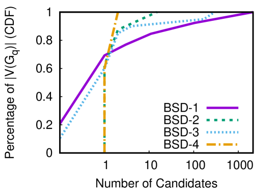
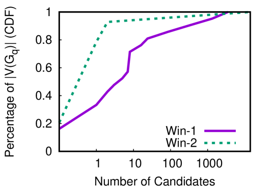
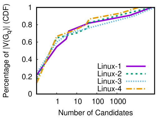
Figure 4. Cumulative Distribution Function (CDF) of number of candidates in $|G_{p}|$ for each node of $|G_{q}|$. From left to right: BSD, Windows, and Linux Scenarios.

We evaluate Poirot’s efficacy and reliability in three different experiments. In the first experiment, we use a set of DARPA Transparent Computing (TC) program red-team vs. blue-team adversarial engagement scenarios which are set up in an isolated network simulating an enterprise network. The setup contains target hosts (Windows, BSD, and Linux) with kernel-audit reporting enabled. During the engagement period, benign background activities were continuously run in parallel to the attacks from the red team.

In the second experiment, we further test Poirot on real-world incidents whose natural language descriptions are publicly available on the internet. To reproduce the attacks described in the public threat reports, we obtained and executed their binary samples in a controlled environment and collected kernel audit logs from which we build the provenance graph. In the third experiment, we evaluate Poirot’s robustness against false signals in an attack-free dataset.

In all the experiments, we set the value of $C_{thr}$ to $3$ (and thus a threshold of $\frac{1}{3}$). This choice is validated in section 5.3. We note, however, that one can configure Poirot with higher or lower values depending on the confidence about the system’s protection mechanisms or the effort cyber-analysts are willing to spend to check the alarms. In fact, the value of $C_{thr}$ influences the number of false positives and potential false negatives. A higher $C_{thr}$ will increase the number of false positives while a lower $C_{thr}$ will reduce it. On the other hand, a higher value of $C_{thr}$ may detect sophisticated attacks, with multiple initial entry points, while a smaller value may miss them. After finding alignment with a score bypassing the threshold, we manually analyzed all the matched attack subgraphs to confirm that they were correctly pinpointing the actual attacks present in the query graphs.

5.1. Evaluation on the DARPA TC Dataset

Scenario	subjects $\in$ |$V(G_{q})$|	objects $\in$ |$V(G_{q})$|	|$E(G_{q})$|	|$F(G_{q})$|
BSD-1	4	9	19	81
BSD-2	1	7	10	32
BSD-3	3	18	34	159
BSD-4	2	8	13	43
Win-1	13	8	26	149
Win-2	1	13	19	94
Linux-1	2	9	19	62
Linux-2	5	12	24	112
Linux-3	2	8	22	48
Linux-4	4	11	22	96

Table 2. Characteristics of Query Graphs.

This experiment was conducted on a dataset released by the DARPA TC program, generated during a red-team vs. blue-team adversarial engagement in April 2018 (Keromytis, 2018). In the engagement, different services were set up, including a web server, an SSH server, an email server, and an SMB server. An extensive amount of benign activities was simulated, including system administration tasks, web browsing to many web sites, downloading, compiling, and installing multiple tools. The red-team relies on threat descriptions to execute these attacks. We obtained these threat descriptions and used them to extract a query graph for each scenario (summary shown in table 2).

In total, we evaluated Poirot on ten attack scenarios including four on BSD, two on Windows, and four on Linux. Due to space restrictions, we are not able to show all the query graphs; however, their characteristics are described in table 2, where subjects indicate processes, and objects indicate files, memory objects, and sockets. BSD-1-4 pertain to attacks conducted on a FreeBSD 11.0 (64-bit) web-server which was running a back-doored version of Nginx. Win-1&2 pertain to attacks conducted on a host machine running Windows 7 Pro (64-bit). The Win-1 scenario contains a phishing email with a malicious Excel macro attachment, while the Win-2 scenario contains exploitation of a vulnerable version of the Firefox browser. Linux1&2 and Linux3&4 pertain to attacks conducted on hosts running Ubuntu 12.04 (64-bit) and Ubuntu 14.04 (64-bit), respectively. Linux1&3 contain in-memory browser exploits, while Linux2&4 involve a user who is using a malicious browser extension.

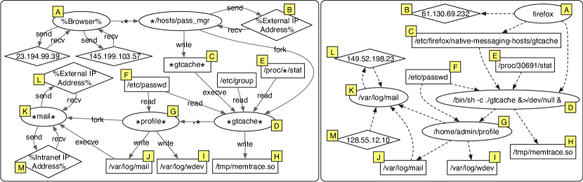
Figure 5. Query Graph of Scenario: Linux-2 (on the left) and its Detected Alignment (on the right).

Scenario	Earliest iteration bypassing threshold	Earliest score bypassing threshold	Max score in 20 iterations	Earliest iteration resulting Max score
BSD-1	1	0.45	0.64	5
BSD-2	1	0.81	0.81	1
BSD-3	1	0.89	0.89	1
BSD-4	1	1	1	1
Win-1	1	0.63	0.63	1
Win-2	1	0.47	0.63	4
Linux-1	1	0.58	0.58	1
Linux-2	2	0.55	0.71	5
Linux-3	1	0.54	0.54	1
Linux-4	1	0.87	0.87	1

Table 3. Poirot’s Graph Alignment Scores.

Alignment Score. As discussed in section 4.2, Poirot iteratively repeats the node alignment procedure starting from the seed nodes with fewer candidates. Figure 4 shows the number of candidate aligned nodes for each node of $G_{q}$. Most of the nodes of $G_{q}$ have less than ten candidate nodes in $G_{p}$, while there are also nodes with thousands of candidate nodes. These nodes, which appear thousands of times, are usually ubiquitous processes and files routinely accessed by benign activities, such as Firefox or Thunderbird. We remind the reader that our seed nodes are chosen first from the nodes with fewer alignments. In each iteration, an alignment is constructed, and its alignment score is compared with the threshold value, which is set to $\frac{1}{3}$.

Table 3 shows Poirot’s matching results for each DARPA TC scenario after producing an alignment of the query graphs with the corresponding provenance graphs. We stop the search after the first alignment that surpasses the threshold value. The second and third columns of table 3 show the number of iterations of the steps 2-4 presented in section 4.2 and the actual score obtained for the first alignment that bypasses the threshold value. In 9 out of 10 scenarios, an alignment bypassing the threshold value was found in the first iteration. In one case, the exact matching of $G_{q}$ could be found in $G_{p}$ (see BSD-4).

The fourth column of table 3 shows the maximum alignment score among the 20 alignments constructed by iterating steps 2-4 of our search algorithm 20 times while the last column shows the earliest iteration-number that resulted in the maximum value. As can be seen, on average, our search converges quickly to a perfect solution. In 7 out of 10 scenarios, the maximum alignment score is calculated in the first iteration, while in the other 3, the maximum alignment scores are calculated in the fourth or fifth iterations. The latter is due to slight differences between the attack reports and the red team’s implementation of the attacks, which result in information flows and causal dependencies that differ slightly between the query graph and the provenance graph. As an example, in Figure 5, we show the query graph and its aligned subgraph for the Linux-2 scenario. In this scenario, the attacker exploits Firefox via a malicious password manager browser extension, to implant an executable to disk. Then, the attacker runs the dropped executable to exfiltrate some confidential information and perform a port scan of known hosts on the target network. We tag the aligned nodes in each graph with the same letter label. Some nodes on the query graph are not aligned with any nodes in the provenance graph. This reduces the score of the graph alignment to a value that is less than 1. Although $G_{q}$ largely overlaps with a subgraph in $G_{p}$, some nodes have no alignment, and some information flows and causal dependencies do not appear in the provenance graph. The percentage of these nodes is small, however. As long as the reports are mainly matching the actual attack activities, our approach will not suffer from this.

5.2. Evaluation on Public Attacks

In this section, we describe the evaluation of Poirot on attacks performed by real-world malware families and compare its effectiveness with that of other similar tools. We show the results of this evaluation in table 4. The names of these malware families, the CTI reports we used as descriptions of their behavior, and the year in which the report is published are shown in the first three columns.

Malware	Report	Year	Reported	Analyzed Malware MD5	Sample	Isolated	Detection Results
Name	Source		Samples		Relation	IOCs	RedLine	Loki	Splunk	Poirot
njRAT	Fidelis (Solutions, 2013)	2013	30	2013385034e5c8dfbbe47958fd821ca0	different	153	F+H	F+H	P	B (score=0.86)
DeputyDog	FireEye (Moran and Villeneuve, 2013)	2013	8	8aba4b5184072f2a50cbc5ecfe326701	subset	21	F$\times 2$+H+R	F$\times 2$+H	P+R	B (score=0.71)
Uroburos	Gdata (Blog, 2013)	2014	4	51e7e58a1e654b6e586fe36e10c67a73	subset	26	F+H	F+H	R	B (score=0.76)
Carbanak	Kaspersky ((GReAT), 2015)	2015	109	1e47e12d11580e935878b0ed78d2294f	different	230	-	PE	S	B (score=0.68)
DustySky	Clearsky (Team, 2016)	2016	79	0756357497c2cd7f41ed6a6d4403b395	different	250	-	-	-	B (score=1.00)
OceanLotus	Eset (by ESET, 2018)	2018	9	d592b06f9d112c8650091166c19ea05a	subset	117	F+R	F+PE	P+R	B (score=0.65)
HawkEye	Fortinet (by FortiGuard Labs, 2019)	2019	3	666a200148559e4a83fabb7a1bf655ac	different	3	-	PE	-	B (score=0.62)

Table 4. Malware reports. In the Detection Results, B=Behavior, PE=PE-Sieve, F=File Name, H=Hash, P=Process Name, R=Registry, S=Windows Security Event.

Mutation Detection Evaluation. As mentioned earlier, a common practice among attackers is that of mutating malware to evade detection or to add more features to it. Therefore, a CTI report may describe the behavior of a different version of the malware that is actually present in the system, and it is vital for a threat hunting tool to be able to detect different mutations of a malware sample. To this end, we execute several real-world malware families, containing different mutated versions of the same malware, in a controlled environment. The fourth column of table 4, shows the number of malware samples with different hash values belonging to the family mentioned in the corresponding CTI report. We note that the reports describe the behavior of only a few samples. The fifth column of table 4 shows our selected sample’s hash value, while the sixth column shows the relation between our selected sample and the ones the CTI report is based on. For instance, the reports of DeputyDog, Uroburos, and OceanLotus cover different activities performed by a set of different samples, and our selected sample is one of them. We have aggregated all those activities in one query graph. For the other test cases, the sample we have executed is different from the ones that the report is based on, which could be considered as detecting a mutated malware. njRAT and DustySky explicitly mention their analyzed sample, which are different from the one we have chosen. The Carbanak report mentions 109 samples, from which we have randomly selected one. Finally, the sample of HawkEye malware is selected from an external source and is not among the samples mentioned in the report.

Comparison with Existing Tools. We compare Poirot with the results of three other tools, namely RedLine(FireEye, 2018b), Loki(Systems, 2017), and Splunk(Splunk, 2019). The input to these tools is extracted from the same report we extract the query graphs and contains IOCs in different types such as hash values, process names, file names, and registries. We have transformed these IOCs to the accepted format of each tool (e.g., RedLine accepts input in OpenIOC format (FireEye, 2018a)). The number of IOCs submitted to Redline, Loki, and Splunk are shown in column-7, while the query graphs submitted to Poirot are shown in LABEL:fig:etw_4_in_one and LABEL:fig:etw_2_in_one. A detailed explanation of these query graphs demonstrating how they are constructed can be found in appendix A. The correspondence between node labels in the query graphs and their actual names is represented in the second and third columns of LABEL:etw-eval-aligns1 and LABEL:etw-eval-aligns2, while the alignments produced by Poirot are shown in the last column.

As shown in the extracted query graphs, the design of Poirot ’s search method, which is based on the information flow and causal dependencies, makes us capable to include benign nodes (nodes C, D, E, and F in DustySky) or attack nodes with exact same names of benign entities (node E in Carbanak) in the query graph. However, these entity names could not be defined as an IOC in the other tested tools as will lead to many false positive alarms. As Redline, Loki, and Splunk look for each IOC in isolation, they expect IOCs as input that are always malicious regardless of their connection with other entities. To this end, we do a preliminary search for each isolated IOC in a clean system and make sure that we have only extracted IOCs that have no match in a clean system. As a result, for some test cases, like HawkEye, although the behavior graph is rich, there are not so many isolated IOCs except a few hash values that could be defined. This highlights the importance of the dependencies between IOCs, which is the foundation of Poirot’s search algorithm, and is not considered by other tools.

Detection Results. The last four columns of table 4 contain the detection results, which show how each tool could detect the tested samples. Keywords B, F, H, P, and R represent detection based on the behavior, file name, hash value, process name, and registry, respectively. In addition, some of the tested tools feature other methods to detect anomalies, injection, or other security incidents. Among these, we encountered some alarms from Windows Security Mitigation and PE-Sieve (hasherezade, 2018), which are represented by keywords S and PE, respectively. While for Poirot, a score is shown which shows the goodness of the overall alignment of each query graph, for the other tools, $\times N$ indicates the number of hits when there has been more than one hit for a specific type of IOC.

As shown in table 4, for all the test cases, Poirot has found an alignment that bypasses the threshold value of $\frac{1}{3}$ . After running the search algorithm, in most of the cases, Poirot found a node alignment for only a subset of the entities in the query graph, except for DustySky, where Poirot found a node alignment for every entity. The information flows and causal dependencies that appear among the aligned nodes are often the same as the query graph with some exceptions. For example, in contrast to how it appears in the query graph of njRAT, where node A generates most of the actions, in our experiment, node F generated most of the actions, such as the write event to nodes C, G, K, L, and the fork event of node I. However, since there is a path from node A to node F in the query graph, Poirot was able to find these alignments and measure a high alignment score.

The samples of njRAT, DeputyDog, Uroburous, and OceanLotus are also detected by all the other tools, as these samples use unique names or hash values that are available in the threat intelligence and could be attributed to those malwares. For the other three test cases, none of the isolated IOCs could be detected because of different reasons such as malware mutations, using random names in each run (nodes J and K in HawkEye query graph), and using legitimate libraries or their similar names. Nevertheless, Splunk found an ETW event related to the Carbanak sample, which is generated when Windows Security Mitigation service has blocked svchost from generating dynamic code. Loki’s PE-Sieve has also detected some attempts of code implants which have resulted in raising some warning signal and not an alert. PE-Sieve detects all modifications done to a process even though they may not necessarily be malicious. As such modifications happen regularly in many benign scenarios, PE-Sieve detections are considered as warning signals that need further investigations.

Conclusions. Our analysis results show that other tools usually perform well when the sample is a subset of the ones the report is written based on. This situation is similar to when there is no mutations, and therefore, there are unique hash values or names that could be used as signature of a malware. For example, DeputyDog sample drops many files with unique names and hash values that do not appear in a benign system, and finding them is a strong indication of this malware. However, its query graph (Figure 2) is not very rich, and Poirot has not been able to correlate the modified registry (node D) with the rest of the aligned nodes. Although the calculated score is still higher than the threshold, but the other tools might perform better when the malware is using well-known IOCs that are strong enough to indicate an attack in isolation.

On the contrary, when the chosen sample is different from the samples analyzed by the report, which is similar to the case that malware is mutated, other tools usually are not able to find the attacks. In such situations, Poirot has a better chance to detect the attack as the behavior often remains constant among the mutations.

Scenario	Size on Disk (Uncompressed)	Consumption time	Occupied Memory	Log Duration	sub $\in$ |$V(G_{p})$|	obj $\in$ |$V(G_{p})$|	|$E(G_{p})$|	Search Time (s)
BSD-1	3022 MB	0h-34m-59s	867 MB	03d-18h-01m	110.66 K	1.48 M	7.53 M	3.28
BSD-2	4808 MB	0h-58m-05s	1240 MB	05d-01h-15m	213.10 K	2.25 M	12.66 M	0.04
BSD-3&4	1828 MB	0h-21m-31s	638 MB	02d-00h-59m	84.39 K	897.63 K	4.65 M	26.09 (BSD-3), 1.47 (BSD-4)
Win-1&2	54.57 GB	4h-58m-30s	3790 MB	08d-13h-35m	1.04 M	2.38 M	70.82 M	125.26 (Win-1), 46.02 (Win-2)
Linux-1&2	9436 MB	1h-26m-37s	4444 MB	03d-04h-20m	324.68 K	30.33 M	51.98 M	1279.32 (Linux-1), 1170.86 (Linux-2)
Linux-3	131.1 GB	2h-30m-37s	21.2 GB	10d-15h-52m	374.71 K	5.32 M	69.89 M	385.16
Linux-4	4952 MB	0h-04m-00s	1095 MB	00d-07h-13m	35.81 K	859.03 K	13.06 M	20.72

Table 8. Statistics of logs, Consumption and Search Times.

5.3. Evaluation on Benign Datasets

To stress-test Poirot on false positives, we used the benign dataset generated as part of the adversarial engagement in the DARPA TC program and four machines (a client, a SSH server, a mail server and a web server) we monitored for one month. Collectively, these datasets contained over seven months worth of benign audit records and billions of audit records on Windows, Linux, and FreeBSD. During this time, multiple users used these systems and typical attack-free actions were conducted including web browsing, installing security updates (including kernel updates), virus scanning, taking backups, and software uninstalls.

After collecting the logs, we run Poirot to construct the provenance graph, and then search for all the query graphs we have extracted from the TC reports and the public malware reports. We try up to 20 iterations starting from different seed node selections per each query graph per each provenance graph and select the highest score. Note that although these logs are attack-free, they share many nodes and events with our query graphs, such as confidential files, critical system files, file editing tools, or processes related to web browsing/hosting, and email clients, all of which were accessed during the benign data collection period. However, even in cases where similar flows appear by chance, the influence score prunes away many of these flows. Consequently, the graph alignment score Poirot calculates among all the benign datasets is at most equal to 0.16, well below the threshold.

Validating the Threshold Value.

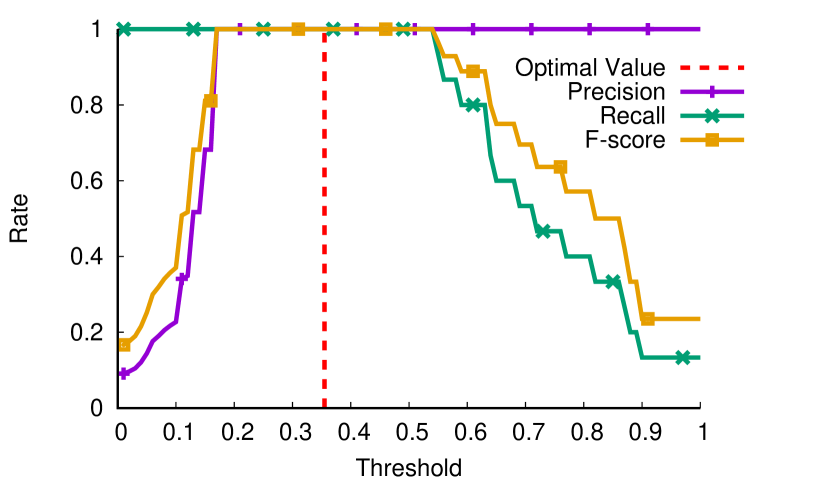
Figure 6. Selecting the Optimal Threshold Value.

The selection of the threshold value is critical to avoid false signals. Too low a threshold could result in premature matching (false positives) while too high a threshold could lead to missing reasonable matches (false negatives). Thus, there is a trade-off in choosing an optimal threshold value. To determine the optimal threshold value, we measured the F-score using varying threshold values, as shown in Figure 6. This analysis is done based on the highest alignment score calculated in 20 iterations of Poirot’s search algorithm for all the attack and benign scenarios we have evaluated. As it is shown, the highest F-score value is achieved when the threshold is at the interval [0.17, 0.54], which is the range in which all attack subgraphs are correctly found, and no alarm is raised for benign datasets. The middle of this interval, i.e., 0.35, maximizes the margin between attack and benign scores, and choosing this value as the optimal threshold minimizes the classification errors,. Therefore, we set the $C_{thr}$ to $3$ which results in $\frac{1}{C_{thr}}=\frac{1}{3}$ which is close to the optimal value.

5.4. Efficiency

Detection	Type	Runtime Overhead			Search
Method		Apache (Apache, 2019)	JetStream (Workbench, 2019)	HDTune (EFD, 2019)	Time (min)
Redline	offline	-	-	-	124
Loki	offline	-	-	-	215
Splunk	online	3.70%	2.94%	4.37%	¡ 1
Poirot	online	0.82%	1.86%	0.64%	¡ 1

Table 7. Efficiency Comparison with Related Systems.

The overheads and search times for the different tools we used are shown in table 7. Redline and Loki are offline tools, searching for artifacts that are left by the attacker on the system, while Splunk and Poirot are online tools, searching based on system events collected during runtime. Hence, Redline and Loki have no runtime overhead due to audit log collection. The runtime overheads of Splunk and Poirot due to log collection are measured using Apache benchmark (Apache, 2019), which measures web server responsiveness, JetStream (Workbench, 2019), which measures browser execution times, and HDTune (EFD, 2019), which measures heavy hard drive transactions. As shown in table 7, both tools have shown negligible runtime overhead, while the runtime of Splunk can be further improved by setting it up in a distributed setting and offloading the data indexing task to another server.

The last column of table 7 shows the time it took searching for IOCs per each tool. The search time of offline tools highly depends on the number of running processes and volume of occupied disk space, which was 500 GB in our case. On the other hand, the search time of online methods highly depends on the log size, type and number of activities represented by the logs. As our experiments with real-world malware samples were running in a controlled environment without many background benign activities and Internet connection, both Splunk and Poirot spend less than one minute to search for all the IOCs mentioned in table 4. In the following, we perform an in-depth analysis of Poirot ’s efficiency on the DARPA TC scenarios, which overall contain over a month worth of log data with combined attack and benign activities. The analysis is done on an 8-core CPU with a 2.5GHz speed each and a 150GB of RAM.

Audit Logs Consumption. In table 8, the second column shows the initial size of the logs on disk, the third column represents the time it takes to consume all audits log events from disk for building the provenance graph in memory. This time is measured as the wall-clock time and varies depending on the size of each audit log and the structure of audits logs generated in each platform (BSD, Windows, Linux). The fourth column shows the total memory consumption by each provenance graph. Comparing the size on disk versus memory, we notice that we have an average compression of 1:4 (25%) via a compact in-memory provenance graph representation based on(Hossain et al., 2017). However, if memory is a concern, it is still possible to achieve better compression using additional techniques proposed in this area (Lee et al., 2013b; Xu et al., 2016; Hossain et al., 2018). The fifth column shows the duration during which the logs were collected while columns 6, 7, and 8 show the total number of subjects (i.e. processes), objects, and events in the provenance graph that is built from the logs, respectively. We note that the query graphs are on average 209K times smaller than the provenance graph for these scenarios. Nevertheless, Poirot is still able to find the exact embedding of $G_{q}$ in $G_{p}$ very fast, as shown in the last column. We note that some scenarios are joined (e.g., Win-1&2) because they were executed concurrently on the same machines.

Graph Analytics. In the last column of table 8, we show the runtime of graph analytics for Poirot’s search algorithm. These times are measured from the moment a search query is submitted until we find a similar graph in $G_{p}$ with an alignment score that surpasses the threshold. Therefore, for Linux-2, the time includes the sum of the times for two iterations. The main bottleneck is on the graph search expansion (Step 3), and the time Poirot spends on graph search depends on several factors. Obviously, the sizes of both query and provenance graph are proportional to the runtime. However, we notice that the node names in $G_{q}$ and the shape of this graph have a more significant effect. In particular, when there are nodes with many candidate alignments, there is a higher chance to reverse the direction multiple times and runtime increases accordingly.

6. Conclusion

Poirot formulates cyber threat hunting as a graph pattern matching problem to reliably detect known cyber attacks. Poirot is based on an efficient alignment algorithm to find an embedding of a graph representing the threat behavior in the provenance graph of kernel audit records. We evaluate Poirot on real-world cyber attacks and on ten attack scenarios conducted by a professional red-team, over three OS platforms, with tens of millions of audit records. Poirot successfully detects all the attacks with high confidence, no false signals, and in a matter of minutes.

Appendix A Appendix

In this section, we provide a brief history of each malware and a summary of the statements from their corresponding reports which we have used to construct the query graphs.

njRAT. njRAT is a publicly available Remote Access Trojan (RAT) that gives the attacker full control over the victim system. Although the source code of njRAT is publicly available, attacks leveraging njRAT have mostly targeted organizations based in or focused on the Middle East region in the government, telecom, and energy sectors. When the malware is executed, it tries to read its configuration from a file with the extension of “.exe.config” (edge 1). njRAT malware stores the logged keystrokes in a “.tmp” file (edge 2), and also writes to a “.pf” file (edge 3). To gain persistence, njRAT malware creates some copies of itself (edges 4&8). After execution (edges 5&6), one of the copies writes to a “.pf” file (edge 7). njRAT malware also start a netsh process located at (edge 9), which results in creation of another “.pf” file (edge 10). Finally, the malware sets some registry values (edges 11-13) and beacons to a C2 server at 217.66.231.245 (edge 14).

DeputyDog. DeputyDog refers to a malware appearing to have targeted organizations in Japan, based on a report by FireEye. The query graph that we extracted from the report of this malware is shown in Figure 2, and it is described in section 3.

Uroburos. Uroburos, ComRAT, Snake, Turla, and Agent.BTZ are all referring to a family of rootkit which is responsible for the most significant breach of U.S. military computers. The malware starts by dropping two Microsoft Windows dynamic libraries (edges 1&2) and calling rundll32.exe (edge 3) to install these libraries (edges 4&5). Then, to be started during the boot process, the malware creates a registry key (edge 6). The malware creates three log files (edges 7-9) and removes a set of file (edges 10-14).

Carbanak. Carbanak is a remote backdoor to provide remote access to infected machines. The main motivation of the attackers appears to be financial gain, which has resulted in cumulative losses up to one billion dollars ((GReAT), 2015). The compromise initially starts using a spear phishing email that appears to be legitimate banking communications (edge 1). After the exploit, Carbanak copies itself into “%system32%” with the name “svchost.exe” (edges 2-4) and deletes the original file created by the exploit payload (edge 5). To access autorun privileges, the malware creates a new service with a name in the format of “¡ServiceName¿Sys”, where ServiceName is any existing service randomly chosen (edge 6). Carbanak creates a file with a random name and a .bin extension where it stores commands to be executed (edge 7). Then, the malware gets the proxy configuration from a registry entry (edge 8) and the Mozilla Firefox configuration file (edge 9). Finally, Carbanak communicates with its C2 server (edge 10).

DustySky. DustySky is a multi-stage malware whose main objective is intelligence gathering for political purposes. The malware sample is disguised as a Microsoft Word file, and once it is executed (edge 1), a lure Microsoft word document in the Arabic language is opened (edges 2&3) while the malware performs intelligence gathering in the background. For VM evasion, the dropper checks the existence of some DLL files, specifically vboxmrxnp.dll and vmbusres.dll which indicate existence of VirtualBox (edges 4&5) and vmGuestlib.dll which indicates existence of VMware (edge 6). DustySky Core is dropped to %TEMP% (edges 7&8&9), and keystroke logs are saved to %TEMP%\temps (edge 10).

OceanLotus. OceanLotus, also known as APT32, is believed to be a Vietnam-based APT group targeting Southeast Asian countries. After execution of this malware (edge 1), a decoy document and an eraser application are dropped (edges 2&3), and the decoy document is lunched in Microsoft Word (edges 4&5). Then, the executable decrypts its resources and drops a copy of legitimate Symantec Network Access Control application (edge 6), an encrypted backdoor (edge 7), and a malicious DLL file (edge 8). The Symantec application, which is signed and legitimate, loads all the libraries in the same folder by default. In this case, after execution (edges 9&10), this application loads the malicious DLL file which has been dropped in the same directory (edge 11). It then reads the backdoor file (edge 12) which results in accessing a registry (edge 13), loading the HTTPProv.dll library (edge 14), and creating a registry key (edge 15). Finally, the malware connects to its mothership (edges 16&17).

HawkEye. HawkEye is a malware-as-a-service credential stealing malware and is a popular tool among APT campaigns. The new variant of this malware uses process hollowing to inject its code into the legitimate signed .NET framework executables and ships with many sophisticated functions to evade detection. This new variant is usually delivered as a compressed file, and after decompression (edges 1&2) and execution(edge 3), it spawns a child process (edge 4), called RegAsm, which is an assembly registration tool from the Microsoft .Net framework. HawkEye extracts a PE file into its memory and then injects it into the RegAsm process. After sleeping for 10 seconds, the RegAsm process spawns two child processes named vbc both from the .Net framework as well (edges 5&6). One of these processes collects credentials of browsers, while the other one focuses on email and Instant Messaging (IM) appllications. We have added one node, typed as a file or registry, corresponding to the name of each browser (edges 7-18) or email/IM (edges 19-26) application mentioned in the report. Note that these applications might store some confidential information of interest to attackers into both files or registries, and that is why we did not limit our search to only files or registries. The collected credentials are regularly saved into $*$.tmp files in the %temp% directory (edges 27&28), while after a while, the RegAsm process reads the entire data of these tmp files into its memory (edges 29&30) and deletes them immediately (edges 31&32). Finally, RegAsm looks up the machines public IP from “http[s]:\\whatismyipaddress.com\” web service (edges 33&34) and then exfiltrates the collected information to the attacker’s email address (edge 35).

It is important to note that there are some nodes with exactly same label and type in the query graph of HawkEye, such as F&G or J&K. However, these nodes get aligned to different nodes based on their dependencies with other entities. For example, node F interacts with browser applications while node G interacts with the email/IM applications. In addition, the alignment of browser or mail application nodes is independent of their installation on the system. Many of these applications are not installed on the test machine, however when the malware attempts to check whether these applications are installed on the system, it initiates an OPEN event which gets detected by Poirot.