Time evolution with symmetric stochastic action

Abstract

The time-evolution of quantum fields is shown to be equivalent to a time-symmetric Fokker-Planck equation. Results are obtained using a Q-function representation, including fermion-fermion, boson-boson and fermion-boson interactions with linear, quadratic, cubic and quartic Hamiltonians, typical of QED and many other cases. For local boson-boson coupling, the resulting probability distribution is proved to have a positive, time-symmetric path integral and action principle, leading to a forward-backward stochastic process in both time directions. The solution corresponds to a c-number field equilibrating in an additional dimension. Paths are stochastic trajectories of fields in space-time, which are samples of a statistical mechanical steady-state in a higher dimensional space. We derive numerical methods and examples of solutions to the resulting stochastic partial differential equations in a higher time-dimension, giving agreement with examples of simple bosonic quantum dynamics. This approach may lead to useful computational techniques for quantum field theory, as well as to new ontological models of physical reality.

I Introduction

The role that time plays in quantum mechanics is a deep puzzle in physics, since quantum measurement appears to preferentially choose a particular time direction, via the projection postulate. This, combined with the Copenhagen interpretation that only macroscopic measurements are real, has led to many quantum paradoxes. Here, we derive a time-symmetric, stochastic quantum action principle to help resolve these issues, extending Dirac’s idea [1] of future-time boundary conditions to the quantum domain. In the cases treated here, quantum field dynamics is shown to be equivalent to a time-symmetric stochastic process. This can be solved by equilibration in the quasi-time of a higher dimensional space, with a genuine probability. There are potentially useful computational consequences, since a quantum action principle with a real exponent has no phase problem. The resulting stochastic trajectories also have an ontological interpretation [2].

The theory uses the Q-function of quantum mechanics [3, 4, 5], which is the expectation value of a coherent state projector. It is a well-defined and positive distribution for any bosonic or fermionic quantum density matrix [6]. In Hamiltonians with up to quartic interactions, the dynamical equation has a time-symmetric Fokker-Planck form. In bosonic cases this is shown to have a zero trace diffusion matrix. There is a quantum action principle for diffusion in positive and negative time-directions simultaneously, equivalent to a time-symmetric stochastic process. The result is time-reversible and non-dissipative, explaining how quantum evolution can be inherently random yet time-symmetric.

Using stochastic bridge theory [7, 8, 9], the Q-function time-evolution is proved to correspond to the steady-state of a diffusion equation in an extra dimension. Thus, stochastic equilibration of a c-number field in five dimensions gives rise to quantum dynamics in four dimensional space-time. This shows that c-number fields in higher dimensions can behave quantum-mechanically. No imaginary-time propagation is required, and the description is probabilistic. The relationship to quantum ontology and measurement theory is given elsewhere [10, 2].

The stochastic fields used here propagate retrocausally as well as in a positive time-direction. Time symmetric evolution was originally proposed by Tetrode in classical electrodynamics [11]. Dirac used the approach to obtain an elegant theory of classical radiation reaction [1], which was extended by Feynman and Wheeler [12]. Time-reversible methods have been studied in quantum physics [13, 14, 15, 16], the philosophy of science [17], and used to explain Bell violations [18]. Here, we use this general approach to analyze interacting fields, thus giving time-symmetric quantum physics a strong foundation.

By comparison, the Fenyes-Nelson approach to stochastic quantum evolution [19, 20], does not have a constructive interpretation [21]. The approach of stochastic quantization [22] uses imaginary time. Such methods have the drawback that analytic continuation to real time dynamics can be intractable [23, 24]. The mathematical technique used here combines the Wiener-Stratonovich stochastic path integral [25, 26], with Schrödinger’s [7] idea of a stochastic bridge in statistical mechanics, as generalized by later workers. The resulting equilibrium is equivalent to quantum dynamics.

All quantum effects are retained in this approach [27]. This is not unexpected, because quantum absorber theory, with similar time-reversed propagation, even has Bell violations [15]. There is a related approach of reciprocal diffusion due to Bernstein [28] and Zambrini [29]. The focus of this paper is to understand quantum dynamics and measurement using stochastic methods. This is important to fundamental applications to quantum measurement theory [2]. In addition, stochastic methods scale well for large systems, which may help to compute exponentially complex many-body dynamics.

Historically, the Kaluza-Klein theory of electromagnetism [30, 31, 32] first introduced a fifth dimension. String theory [33, 34], as well as the Randall-Sundrum [35] and Gogberashvili [36] approach to the hierarchy problem all use extra dimensions. As with these approaches, one can usefully visualize the extra dimensions as real extensions of space-time. In the theory presented here, the extra dimension is time-like and non-compact. Just as in ‘flatland’ [37], the location of observers defines the extra coordinate. However, our results only make use of an extra dimension as a computational tool, so this is not essential to the physical interpretation.

Quantum dynamical problems arise in many fields, from many-body theory to cosmology. The utility of the path integral derived here is that it is real, not imaginary [38]. Other methods exist for quantum dynamics. These include mean field theory, perturbation theory, variational approaches [39], standard phase-space methods [4] and the density matrix renormalization group [40]. Each has its own drawbacks, however. The time-symmetric techniques given here use a different approach, as well as providing a model for a quantum ontology.

To demonstrate these results, a general quartic quantum field Hamiltonian is introduced. This corresponds to common quantum models, including QED, Bose-Hubbard, Fermi-Hubbard, Ising, quantum circuit and parametric Hamiltonians. The corresponding Q-function dynamics satisfies a time-symmetric Fokker-Planck equation in all cases. Further extensions of the Q-function method would be required to treat the bosonic sector in QCD. Such Hamiltonians are closely related to the classes treated here. The common feature is that they have a cubic or quartic interaction term. In the boson-boson and boson-fermion cases it is shown that there is a zero trace diffusion. A detailed treatment is given of the simplest boson-boson case. This leads to a time-symmetric stochastic differential equations, a quantum action principle and a probabilistic path integral. A solution is obtainable through positive diffusion in a higher dimension. Elementary examples and numerical solutions are obtained. Results are compared with exactly soluble cases.

The content of this paper is as follows. Section II derives properties of Q-functions and time-symmetric Fokker-Planck equations, proving that there is a traceless diffusion matrix for boson-boson and fermion-boson quantum field theories. Section III defines quantum trajectories and an action principle using time-symmetric stochastic equations. Section IV shows that the resulting real path integral is equivalent to a Q-function time-evolution. Section V treats extra dimensions, and shows how the classical limit is regained. Section VI gives examples and numerical results. Finally, section VII summarizes the paper.

II Q-functions

Phase-space representations in quantum mechanics allow efficient treatment of quantum systems via probabilistic sampling [41]. These general methods are related to coherent states [42] and Lie groups [43], which introduce a continuous set of parameters in Hilbert space. Results for bosonic and fermionic fields are summarized below. Q-functions [3] can also be used for spins [44, 45] but this is essentially a subset of the results given here.

The Q-function is probabilistic and defined in real time. Yet it does $not$ have a traditional stochastic interpretation, since unitary evolution can generate diffusion terms that are not positive-definite [46]. An earlier method of treating this was to double the phase-space dimension to give a positive diffusion [47]. This is usually applied to normal ordering [42], but the corresponding distribution is non-unique, and is most useful for damped systems [48] or short times [49, 50, 51]. With undamped systems however, doubling phase-space gives sampling errors that increase with time [52, 53]. Rather than using this earlier approach, a positive diffusion is obtained here through equilibration in an extra space-time dimension.

II.1 General definition of a Q-function

The general abstract definition of a Q-function [6] is:

$$Q(\bm{\lambda},t)=Tr\left\{\hat{\Lambda}\left(\bm{\lambda}\right)\hat{\rho}\left(t\right)\right\}\,,$$ (1)

where $\hat{\rho}\left(t\right)$ is the quantum density matrix, $\hat{\Lambda}\left(\bm{\lambda}\right)$ is a positive-definite operator basis, and $\bm{\lambda}$ is a point in phase-space with an integration measure $d\bm{\lambda}$ such that the identity operator $\hat{I}$ can be expanded as:

$$\hat{I}=\int\hat{\Lambda}\left(\bm{\lambda}\right)d\bm{\lambda}\,.$$ (2)

Provided $\hat{\rho}\left(t\right)$ is normalized in the standard way so that $Tr\left[\hat{\rho}\left(t\right)\right]=1$, the Q-function is positive and normalized to unity:

$$\int d\bm{\lambda}Q\left(\bm{\lambda}\right)=1\,.$$ (3)

This satisfies the requirements of a probability. The basis function $\hat{\Lambda}\left(\bm{\lambda}\right)$ does not project the eigenstates of a Hermitian operator, and therefore the quantum dynamical equations differ from those for orthogonal eigenstates.

Quantum fields are defined with an $n_{d}$-dimensional space-time coordinate $r$, where $r=\left(r^{1},\ldots r^{n_{d}}\right)=\left(\bm{r},t\right)$. The fields can be expanded using $M_{b}$ bosonic annihilation and creation operators $\hat{a}_{i},\hat{a}_{i}^{\dagger}$ and $M_{f}$ fermionic operators $\hat{b}_{i},\hat{b}_{i}^{\dagger}$. The internal indices $i$ may include $N_{b}$ ($N_{f}$) internal degrees of freedom like spin or charm, for $M_{b}/N_{b}$ and $M_{f}/N_{f}$ spatial modes respectively, each of which describe excitations on a lattice or single-particle eigenmodes.

As a result, the corresponding phase-space coordinate $\bm{\lambda}=\left(\bm{\alpha},\underline{\underline{\xi}}\right)$ has both fermionic and bosonic amplitudes, and the basis function $\hat{\Lambda}\left(\bm{\lambda}\right)$ is a product of fermionic and bosonic operators, so that:

$$\hat{\Lambda}\left(\bm{\lambda}\right)=\prod_{b,f}\hat{\Lambda}_{b}\left(\bm{\alpha}\right)\hat{\Lambda}_{f}\left(\underline{\underline{\xi}}\right).$$ (4)

We now briefly recall the properties of the basis operators, $\hat{\Lambda}_{b}\left(\bm{\alpha}\right)$ and $\hat{\Lambda}_{f}\left(\underline{\underline{\xi}}\right)$. For simplicity we assume one bosonic and/or one fermionic field here, noting that there may be more than one species labeled $b,f$ if there are conservation laws. They must satisfy the completeness condition, Eq (2). The basis is not orthogonal, and it is generally essential to employ non-orthogonal bases and Lie group theory in order to obtain differential and integral identities.

For bosonic fields, $\hat{\Lambda}_{b}$ is proportional to a coherent state projector [42],

$$\hat{\Lambda}_{b}\left(\bm{\alpha}\right)\equiv\left|\bm{\alpha}\right\rangle_{c}\left\langle\bm{\alpha}\right|_{c}/\pi^{M_{b}}.$$ (5)

The state $|\bm{\alpha}\rangle_{c}$ is a normalized Bargmann-Glauber [54, 42] coherent state with $\hat{a}_{i}|\bm{\alpha}\rangle_{c}=\alpha_{i}|\bm{\alpha}\rangle_{c}$ and $\hat{\bm{\psi}}\left(\bm{r}\right)|\bm{\alpha}\rangle_{c}=\bm{\psi}\left(\bm{r}\right)|\bm{\alpha}\rangle_{c}$, where $\bm{\alpha}$ is an $M_{b}$-dimensional complex vector of coherent field mode amplitudes and $\bm{\psi}\left(\bm{r}\right)$ is the corresponding coherent field. Here, Latin indices $i,j,k,\ell$ are summed up to $M_{b}$, with bold vectors and matrices. On Fourier transforming to position space, $Q\left[\bm{\psi}\right]$ in field space is a functional of the complex field amplitudes $\bm{\psi}\left(\bm{r}\right)$ [55, 56].

For fermionic fields, the Gaussian operator $\hat{\Lambda}_{f}$ is given in the Majorana representation by [57, 58]

$$\hat{\Lambda}_{f}\left(\underline{\underline{\xi}}\right)=\mathcal{N}\left(\underline{\underline{\xi}}\right):\exp\Biggl{[}-i\hat{\underline{\gamma}}^{T}\left[\underline{\underline{i}}-\underline{\underline{i}}\left(\underline{\underline{i}}\underline{\underline{\xi}}+\underline{\underline{I}}\right)^{-1}\right]\hat{\underline{\gamma}}/2\Biggr{]}.$$ (6)

The fermionic $\underline{\underline{\xi}}$ coordinates are real antisymmetric $2M_{f}\times 2M_{f}$ matrices with an integration measure $d\underline{\underline{\xi}}=\prod_{m<n}d\xi_{mn}$, and an integration domain such that $\left(\underline{\underline{\xi}}^{2}+\underline{\underline{I}}\right)$ is a positive semi-definite matrix. Latin indices $m,n,o,p$ for extended vectors are summed up to $2M_{f}$, with underlined vectors and matrices. The normalization factor is $\mathcal{N}\left(\underline{\underline{\xi}}\right)=2^{-M_{f}}\sqrt{\det\left[\underline{\underline{i}}-\underline{\underline{\xi}}\right]}$, where

$$\underline{\underline{i}}=\left[\begin{array}[]{cc}\mathbf{0}&\mathbf{\mathbf{I}}\\ -\mathbf{I}&\mathbf{0}\end{array}\right].$$ (7)

Here $\underline{\underline{I}}$ is a $2M_{f}\times 2M_{f}$ identity matrix, $\mathbf{\mathbf{I}}$ is an $M_{f}\times M_{f}$ identity matrix, and $\hat{\underline{\gamma}}$ is a vector of Majorana operators with commutators

$$\left\{\hat{\gamma}_{m},\hat{\gamma}_{n}\right\}=2\delta_{mn}.$$ (8)

The Majorana operators are obtained using a matrix transformation [59] $\underline{\underline{U}}=\left[\begin{array}[]{cc}\mathbf{I}&\mathbf{I}\\ -i\mathbf{I}&i\mathbf{I}\end{array}\right]$, acting on a vector of extended fermionic creation and annihilation operators, $\hat{\underline{b}}=\left(\hat{\bm{b}}^{T},\hat{\bm{b}}^{\dagger}\right)^{T}$, so that $\hat{\underline{\gamma}}=\underline{\underline{U}}\hat{\underline{b}}.$ There are $M_{f}\left(2M_{f}-1\right)$ independent fermionic phase-space variables, owing to antisymmetry.

II.2 Observables

Quantum expectations $\left\langle\hat{O}\right\rangle$ of ordered observables $\hat{O}$ are identical to probabilistic Q-function averages $\left\langle O\right\rangle_{Q}$, including corrections for operator re-ordering if necessary:

$$\left\langle\hat{O}\right\rangle=\left\langle O\right\rangle_{Q}\equiv\int d\bm{\lambda}Q\left(\bm{\lambda}\right)O(\bm{\lambda})\,.$$ (9)

Here, $\left\langle\right\rangle$ indicates a quantum expectation value, $\left\langle\right\rangle_{Q}$ is a Q-function phase-space probabilistic average, and time-arguments are implicit.

In the bosonic case, the expectation of any observable $\hat{O}$ is obtained by first expanding $\hat{\rho}$ in a generalized P-representation, $P\left(\alpha,\beta\right)$. This always exists [60], so that for any quantum density matrix $\hat{\rho}$,

$$\hat{\rho}=\int P\left(\bm{\alpha},\bm{\beta}\right)\hat{\Lambda}_{p}\left(\bm{\alpha},\bm{\beta}\right)d\bm{\alpha}d\bm{\beta}\,,$$ (10)

where $\hat{\Lambda}_{p}\left(\bm{\alpha},\bm{\beta}\right)$ is an off-diagonal coherent projector,

$$\hat{\Lambda}_{p}\left(\bm{\alpha},\bm{\beta}\right)=\frac{\left|\bm{\alpha}\right\rangle_{c}\left\langle\bm{\beta}\right|_{c}}{\left\langle\bm{\beta}\right.\left|\bm{\alpha}\right\rangle_{c}}\,.$$ (11)

We use $d\bm{\alpha}$, $d\bm{\beta}$ to denote $M$ dimensional complex integration measures, so that if $\bm{\alpha}=\bm{q}+i\bm{p}$, then $d\bm{\alpha}=d\bm{q}d\bm{p}\equiv d^{M}\bm{q}d^{M}\bm{p}$. The existence proof [60] shows that there is a canonical probability distribution $P\left(\bm{\alpha},\bm{\beta}\right)$ which is obtained from the Q-function:

$$P\left(\bm{\alpha},\bm{\beta}\right)=\left(\frac{1}{4\pi}\right)^{M}\exp\left[-\frac{\left|\bm{\alpha}-\bm{\beta}\right|^{2}}{4}\right]Q\left(\frac{\bm{\alpha}+\bm{\beta}}{2}\right)\,.$$ (12)

This can be used to invert the Q-function representation mapping, to obtain the general operator correspondence function for $\hat{O}$ in the form of an integration over $\bm{\alpha}$:

$$\left\langle\hat{O}\right\rangle\equiv\text{{\hbox{\int}}d{\hbox{\bm{\alpha}Q^{\alpha}\left(\bm{\alpha}\right)}}O{\hbox{\left(\bm{\alpha}\right)}}}=\left\langle O\right\rangle_{Q}.$$ (13)

To prove this, we use the expansion of $\hat{\rho}$ in Eq (10), which gives that:

$$\left\langle\hat{\sigma}\right\rangle_{Q}\equiv\int P\left(\bm{\beta},\bm{\gamma}\right)Tr\left[\hat{O}\hat{\Lambda}_{p}\left(\bm{\beta},\bm{\gamma}\right)\right]d\bm{\beta}d\bm{\gamma}\,.$$ (14)

Expanding this using the canonical expansion, Eq (12), the c-number function corresponding to $\hat{O}$ is therefore $O\left(\bm{\alpha}\right)$, where on defining $\bm{\alpha}=\left(\bm{\beta}+\bm{\gamma}\right)/2$, $\bm{\Delta}=\left(\bm{\beta}-\bm{\gamma}\right)/2$:

$$O\left(\bm{\alpha}\right)=\frac{1}{\pi^{M}}\int e^{-\left|\Delta\right|^{2}}Tr\left[\hat{O}\hat{\Lambda}_{p}\left(\bm{\alpha}+\bm{\Delta},\bm{\alpha}-\bm{\Delta}\right)\right]d\bm{\Delta}\,.$$ (15)

As an example, particle numbers in the bosonic case are given by introducing the equivalent c-number function $n\left(\alpha\right)\equiv\left|\alpha\right|^{2}-1$, so that the quantum and probabilistic averages agree:

$$\left\langle\hat{n}\right\rangle=\left\langle n\left(\alpha\right)\right\rangle_{Q}=\left\langle\left|\alpha\right|^{2}-1\right\rangle_{Q}.$$ (16)

This is a special case of the general identity given above. As another example, a $p-th$ order anti-normally ordered moment is

$$\left\langle\hat{a}_{i1}\ldots\hat{a}_{i_{p}}^{\dagger}\right\rangle =\left\langle\alpha_{i_{1}}\ldots\alpha_{i_{p}}^{*}\right\rangle_{Q}.$$ (17)

These operator moments can be of any order $p$.

Similar techniques are available for fermions [6] and spins [44, 45], so this approach is not restricted to bosonic fields. As emphasized in Dirac’s review paper [61], one can calculate any observable average from a quasi-distribution, provided the observable is expressed in terms of a suitable operator ordering. In the bosonic case, it is the anti-normal ordering of ladder operators that is utilized for Q-functions.

II.3 Identities and exact results

There are several mathematical properties that make this expansion a useful approach. We first introduce a shorthand notation for differential operators, $\partial_{i}\equiv\partial/\partial\alpha_{i}$. For convenience in treating products of less than four boson operators a convention of defining $\hat{a}_{0}=1=\alpha_{0}$ and $\partial_{0}\equiv 0$ is used.

The following operator correspondences for bosons hold for the unit terms with zero index as well as for operators:

$$\hat{a}_{j}\hat{\Lambda} = \alpha_{j}\hat{\Lambda}$$

$$\hat{\Lambda}\hat{a}_{j}^{\dagger} = \alpha_{j}^{*}\hat{\Lambda}$$

$$\hat{a}_{j}^{\dagger}\hat{\Lambda} = \left(\partial_{j}+\alpha_{j}^{*}\right)\hat{\Lambda}$$

$$\hat{\Lambda}\hat{a}_{j} = \left(\partial_{j}^{*}+\alpha_{j}\right)\hat{\Lambda}.$$ (18)

For $j=0$, the first two identities are trivial since $\hat{a}_{0}=\alpha_{0}$. The last two follow immediately, since because $\partial_{0}\equiv 0$ , these are simply conjugates of the first two identities.

To illustrate that this introduces no contradictions, note that for operator products, the differential identities give the following result for a commutator:

$$\left[\hat{a}_{i},\hat{a}_{j}^{\dagger}\right]\hat{\Lambda} =\left[\partial_{j},\alpha_{i}\right]\hat{\Lambda}$$

$$\hat{\Lambda}\left[\hat{a}_{i},\hat{a}_{j}^{\dagger}\right] =\left[\partial_{i}^{*},\alpha_{j}^{*}\right]\hat{\Lambda}.$$ (19)

These identities give the result that $\left[\hat{a}_{i},\hat{a}_{j}^{\dagger}\right]\hat{\Lambda}=\delta_{ij}\hat{\Lambda}$ if $i,j>0$, as required for an operator. If one of $i,j$ are zero, then the commutator identity vanishes, as it must for a c-number. The resulting identities have the same form as for the usual annihilation and creation operators. This allows linear, quadratic and cubic terms to be treated in a uniform formalism. Einstein summations over $i,j\ldots=0,\ldots M_{b}$, and $m,n=1,\ldots 2M_{f}$ will be included implicitly for repeated indices.

There are the following operator correspondences for bosons [42, 62, 63, 5]:

$$\hat{a}_{i}\hat{a}_{j}^{\dagger}\hat{\Lambda} = \left(\partial_{j}+\alpha_{j}^{*}\right)\alpha_{i}\hat{\Lambda}$$

$$\hat{\Lambda}\hat{a}_{i}\hat{a}_{j}^{\dagger} = \left(\partial_{i}^{*}+\alpha_{i}\right)\alpha_{j}^{*}\hat{\Lambda}.$$ (20)

Using an anti-normally ordered product notation for Bose operators, $\hat{\mathcal{B}}_{ij}=\hat{a}_{i}\hat{a}_{j}^{\dagger}$, these generally applicable identities can be written in terms of differential operators $\mathcal{B}_{ij}$ and $\bar{\mathcal{B}}_{ij}$ as:

$$\hat{\mathcal{B}}_{ij}\hat{\Lambda} =\mathcal{B}_{ij}\hat{\Lambda}$$

$$\hat{\Lambda}\hat{\mathcal{B}}_{ij} =\bar{\mathcal{B}}_{ij}\hat{\Lambda}.$$ (21)

Such results also hold for fermions, except that only quadratic and quartic fermionic terms occur, so that there is no need to treat odd numbers of operators. We introduce $\partial_{nm}\equiv\partial/\partial\zeta_{mn}$, where $\partial_{nm}$ is a structured derivative for antisymmetric matrices such that $\partial_{nm}\xi_{m^{\prime}n^{\prime}}=\delta_{nn^{\prime}}\delta_{mm^{\prime}}-\delta_{nm^{\prime}}\delta_{mn^{\prime}}$, and $\zeta_{mn}$ is the fermionic phase-space matrix from Eq (6). Defining $\underline{\underline{\xi}}^{\pm}=\underline{\underline{\xi}}\pm i\underline{\underline{I}}$ , the following identities are known [58]:

$$\hat{\gamma}_{m}\hat{\gamma}_{n}\hat{\Lambda} = i\left(\xi_{mm^{\prime}}^{-}\xi_{n^{\prime}n}^{+}\partial_{m^{\prime}n^{\prime}}-\xi_{mn}^{+}\right)\hat{\Lambda}$$

$$\hat{\Lambda}\hat{\gamma}_{m}\hat{\gamma}_{n} = i\left(\xi_{mm^{\prime}}^{+}\xi_{n^{\prime}n}^{-}\partial_{m^{\prime}n^{\prime}}-\xi_{mn}^{+}\right)\hat{\Lambda}.$$ (22)

Introducing quadratic Fermi operators $\mathcal{\hat{F}}_{mn}=\hat{\gamma}_{m}\hat{\gamma}_{n}$ and their corresponding differential operators $\mathcal{F}_{mn}$ and $\bar{\mathcal{F}}_{mn}$, one can write this as

$$\mathcal{\hat{F}}_{mn}\hat{\Lambda} = \mathcal{F}_{mn}\hat{\Lambda}$$

$$\hat{\Lambda}\mathcal{\hat{F}}_{mn} = \bar{\mathcal{F}}_{mn}\hat{\Lambda}.$$ (23)

Q-function evolution equations are obtained by using these operator identities to change Hilbert space operators acting on $\hat{\rho}$ to differential operators acting $\hat{\Lambda}$, and hence on $Q$. To obtain operator product identities for quartic terms, one uses the fact that the mode operators commute with the c-number terms, so that the operator closest to the kernel $\hat{\Lambda}$ always generates a differential term that is furthest from $\hat{\Lambda}$. In the fermionic case one must choose a defined index ordering, for example $m<n$, and use antisymmetry with $\xi_{nm}=-\xi_{mn}$, so that there are only independent variables in the phase-space.

As a typical example, one obtains:

$$\hat{\mathcal{B}}_{ij}\hat{\mathcal{B}}_{kl}\hat{\Lambda} =\mathcal{B}_{kl}\mathcal{B}_{ij}\hat{\Lambda}$$

$$\hat{\Lambda}\hat{\mathcal{B}}_{ij}\hat{\mathcal{B}}_{kl} =\bar{\mathcal{B}}_{ij}\bar{\mathcal{B}}_{kl}\hat{\Lambda}.$$ (24)

Exact Q-functions are known for a number of special cases, including all gaussian states. For brevity we focus on bosonic examples, as fermionic cases are treated elsewhere [64, 65, 6]. A noninteracting multi-mode vacuum state, $\left|\bm{0}\right\rangle$, and more generally a coherent state $\left|\bm{\alpha}_{0}\right\rangle_{c}$, where $\bm{\alpha}_{0}\equiv\bm{0}$ in the vacuum state, has the Q-function

$$Q^{\alpha}\left(\bm{\alpha}\right)=\frac{1}{\pi^{M}}\exp\left(-\left|\bm{\alpha}-\bm{\alpha}_{0}\right|^{2}\right)\,.$$ (25)

This has a well known interpretation [66, 67]. If one makes a simultaneous measurement of two orthogonal quadratures, which is possible using a beam-splitter, then $Q\left(\bm{\alpha}\right)$ is the probability of a simultaneous measurement of quadratures $q$ and $p$, where $\alpha=q+ip$. This is also the result of an amplified measurement [68].

Any number state $\left|\Psi\right\rangle=\left|\bm{n}\right\rangle$ has a representation as:

$$Q^{\alpha}\left(\bm{\alpha}\right) =\frac{1}{\pi^{M}}e^{-\left|\bm{\alpha}\right|^{2}}\prod_{i}\left[\sum_{n_{i}}\frac{\left|\alpha_{i}\right|^{2n_{i}}}{n_{i}!}\right].$$ (26)

A free-particle thermal state with mean particle number $\bm{n}^{th}$ has a Gaussian Q-function given by:

$$Q^{\alpha}\left(\bm{\alpha}\right)=\prod_{i}\frac{1}{\pi\left(1+n_{i}^{th}\right)}e^{-\left|\alpha_{i}\right|^{2}/\left(1+n_{i}^{th}\right)}.$$ (27)

II.4 Quantum field dynamics

To understand dynamics, we consider a time-dependent multi-mode Hamiltonian with quartic, cubic, quadratic and linear terms. This Hamiltonian is then expanded using mode operators. In the present treatment, although number conserving nonlinear bosonic terms like $\hat{a}^{\dagger 2}\hat{a}^{2}$ are included, we exclude non-number-conserving cubic or quartic terms in bosonic operators like $\hat{a}^{4}$. This removes self-interacting real scalar bosonic fields and related Hamiltonians in the standard model.

The models covered are applicable to many experimentally tested fundamental as well as common effective Hamiltonians, including QED, Bose and Fermi Hubbard models, the Ising model, parametric amplifiers and quantum circuits. The QCD interaction Hamiltonian has a quartic self-interaction term for Yang-Mills bosons [69]. This would require a Q-function involving Gaussian bosonic operators [70] which is not treated here.

A simple example is the QED interaction Hamiltonian, of form $\hat{\psi}_{i}\hat{A}^{\rho}\hat{\psi}_{j}$, where $\hat{\bm{\psi}}$ is a relativistic Fermi field and $\hat{\bm{A}}$ is the electromagnetic potential. After expanding in annihilation and creation operators, this leads to terms of the form $\hat{\mathcal{B}}_{ij}\hat{\mathcal{F}}_{mn}$ in our notation. Including all the presently allowed combinations of fermionic and bosonic fields gives:

$$\hat{H}\left(t\right) =\hat{H}_{B}\left(t\right)+\hat{H}_{FB}\left(t\right)+\hat{H}_{F}\left(t\right),$$ (28)

where the different types of Hamiltonian are:

$$\hat{H}_{B}\left(t\right) \equiv\frac{\hbar}{2}g_{ijkl}^{B}\left(t\right)\hat{\mathcal{B}}_{ij}\hat{\mathcal{B}}_{kl}$$

$$\hat{H}_{FB}\left(t\right) \equiv\frac{\hbar}{2}g_{ijmn}^{FB}\left(t\right)\hat{\mathcal{B}}_{ij}\hat{\mathcal{F}}_{mn}$$

$$\hat{H}_{F}\left(t\right) \equiv\frac{\hbar}{2}g_{mnop}^{F}\left(t\right)\hat{\mathcal{F}}_{mn}\hat{\mathcal{F}}_{op}\,.$$ (29)

While formally quartic, these Hamiltonians include linear, quadratic and cubic bosonic Hamiltonians as well, through the bosonic terms that involve $\hat{a}_{0}$. The quadratic case includes all bosonic and fermionic free-field Hamiltonians, both relativistic and non-relativistic, because we have defined $\hat{\mathcal{B}}_{00}=\hat{a}_{0}\hat{a}_{0}^{\dagger}=\hat{1}$. The time argument of $g\left(t\right)$ is not written explicitly from now on, but it is understood to apply. Renormalization is carried out through cutoff dependent coupling constants.

As $\hat{H}$ is hermitian, the following constraints must be imposed on the coupling matrices:

$$g_{ijkl}^{B} =g_{lkji}^{B*}$$

$$g_{ijmn}^{FB} =g_{jinm}^{FB*}$$

$$g_{mnop}^{F} =g_{ponm}^{F*}\,.$$ (30)

Without loss of generality, we also assume a permutation symmetry with

$$g_{ijkl}^{B} =g_{klij}^{B}$$

$$g_{mnop}^{F} =g_{opmn}^{F}.$$ (31)

Cubic bosonic Hamiltonians such as $\hat{a}_{0}\hat{a}_{j}\hat{a}_{k}^{\dagger}\hat{a}_{l}^{\dagger}=\hat{a}_{j}\hat{a}_{k}^{\dagger}\hat{a}_{l}^{\dagger}$ are also of this general form. These describe parametric couplings found in quantum science, and are used in low-noise amplifiers for quantum measurements [71]. While not all quantum field Hamiltonians in the standard model can be analyzed without further extensions to the representation, the class of Hamiltonians that is covered is both very large and applicable to much of current quantum physics.

Quantum dynamics is described by the Schrödinger equation, which is

$$i\hbar\frac{d\hat{\rho}}{dt}=\left[\hat{H},\hat{\rho}\right].$$ (32)

The corresponding dynamical evolution of the Q-function for unitary evolution is given by

$$\frac{dQ}{dt} =\frac{i}{\hbar}Tr\left\{\left[\hat{H},\hat{\Lambda}\left(\bm{\alpha}\right)\right]\hat{\rho}\right\}.$$ (33)

After implementing the mappings given above, one obtains three types of differential operator acting on Q:

$$\frac{dQ}{dt}=\left[\mathcal{L}_{B}+\mathcal{L}_{FB}+\mathcal{L}_{F}\right]Q.$$ (34)

The identities of Eq (20) and (24) give for boson-boson coupling, found in the Bose-Hubbard models:

$$\mathcal{L}_{B} =\frac{i}{2}g_{ijkl}^{B}\left[\left(\partial_{l}+\alpha_{l}^{*}\right)\alpha_{k}\left(\partial_{j}+\alpha_{j}^{*}\right)\alpha_{i}\right.$$

$$\left.-\left(\partial_{i}^{*}+\alpha_{i}\right)\alpha_{j}^{*}\left(\partial_{k}^{*}+\alpha_{k}\right)\alpha_{l}^{*}\right].$$ (35)

For boson-fermion coupling, one obtains from Eq (22):

$$\mathcal{L}_{FB} =\frac{-1}{2}g_{ijmn}^{FB}\left[\left(\partial_{j}+\alpha_{j}^{*}\right)\alpha_{i}\left(\xi_{mm^{\prime}}^{-}\xi_{n^{\prime}n}^{+}\partial_{m^{\prime}n^{\prime}}-\xi_{mn}^{+}\right)\right.$$

$$\left.-\left(\partial_{i}^{*}+\alpha_{i}\right)\alpha_{j}^{*}\left(\xi_{mm^{\prime}}^{+}\xi_{n^{\prime}n}^{-}\partial_{m^{\prime}n^{\prime}}-\xi_{mn}^{+}\right)\right].$$ (36)

The case of fermion-fermion coupling, as in the Fermi-Hubbard model, gives:

$$\mathcal{L}_{F} =\frac{-i}{2}g_{mnop}^{F}\left[\left(\xi_{oo^{\prime}}^{-}\xi_{p^{\prime}p}^{+}\partial_{o^{\prime}p^{\prime}}-\xi_{op}^{+}\right)\times\right.$$

$$\times\left(\xi_{mm^{\prime}}^{-}\xi_{n^{\prime}n}^{+}\partial_{m^{\prime}n^{\prime}}-\xi_{mn}^{+}\right)$$

$$\left.-\left(\xi_{mm^{\prime}}^{+}\xi_{n^{\prime}n}^{-}\partial_{m^{\prime}n^{\prime}}-\xi_{mn}^{+}\right)\left(\xi_{oo^{\prime}}^{+}\xi_{p^{\prime}p}^{-}\partial_{o^{\prime}p^{\prime}}-\xi_{op}^{+}\right)\right].$$

The antisymmetry of $\xi_{mn}$ means that one must use the identity that $\partial_{nm}=-\partial_{mn}$ in order to restrict summations of derivatives so that only independent fermionic variables are summed over, with $m<n$. One can include decoherence and reservoirs by adding them to the Hamiltonian. Such reservoirs can be included in the dynamical equations, thus enlarging both the Hilbert space and the phase space dimension. As a result, unitary evolution is not a limitation.

Next, define an extended vector $\vec{\alpha}=\alpha^{\mu}$, where $\alpha^{j}=\alpha_{j}$, $\alpha^{j+M_{b}}=\alpha_{j}^{*}$, $\partial_{j+M_{b}}=\partial_{j}^{*}$, which includes amplitudes and conjugates. If fermions are present, one must take account of matrix antisymmetry, to include the fermionic variables. To treat this, for indices $\rho>2M_{b}$, we define extended indices $\rho(m,n)$ so that $\alpha^{\rho(m,n)}=\xi_{mn}$, where $m<n$ and $\rho(m,n)=2M_{b}+m+(n-1)(n-2)/2$.

This gives a total index range of $M=2M_{b}+M_{f}\left(2M_{f}-1\right)$. Using an implicit Einstein summation convention, over $\mu,\nu=1,\ldots M$, and noting that constant terms cancel due to the conservation of probability, one obtains a complex time-symmetric Fokker-Planck equation (TFPE) where:

$$\frac{dQ}{dt} =\left[\mathcal{L}_{B}+\mathcal{L}_{FB}+\mathcal{L}_{F}\right]Q$$

$$=\left[-\frac{\partial}{\partial\alpha^{\nu}}A_{\alpha}^{\nu}\left(\vec{\alpha}\right)+\frac{1}{2}\frac{\partial}{\partial\alpha^{\mu}}\frac{\partial}{\partial\alpha^{\nu}}D_{\alpha}^{\mu\nu}\left(\vec{\alpha}\right)\right]Q.$$ (37)

From Eq (35) and (20), the diffusion term for the bosonic case $\mathcal{L}_{B}$, with $1\leq l,j\leq M$ is:

$$D_{\alpha}^{lj}\left(\vec{\alpha},t\right) =i\sum_{i,k=0}^{M}g_{ijkl}^{B}\alpha_{i}\alpha_{k}\,\,.$$ (38)

Letting $l^{\prime},j^{\prime}\equiv l+M,j+M$, one sees that

$$D_{\alpha}^{lj}=D_{\alpha}^{l^{\prime}j^{\prime}*},$$ (39)

and for unitary evolution there are no cross-terms $D_{\alpha}^{lj^{\prime}}$. Generally, the second-order coefficient $D_{\alpha}^{\mu\nu}\left(\vec{\alpha}\right)$ depends on the extended phase-space location $\vec{\alpha}$. In cases of purely quadratic Hamiltonians, the diffusion is either zero or constant in phase-space.

II.5 Traceless diffusion and time-reversibility

For unitary quantum evolution, the diffusion matrix is divided into two parts, one positive definite and one negative definite, corresponding to diffusion in the forward and backward time directions respectively. To prove this, we first show that the corresponding Q-function time-evolution has a TFPE with a traceless diffusion matrix. That is, unlike standard diffusion equations, we will prove that the Q-function dynamical equation has an equal weight of positive and negative diagonal diffusion terms.

For length reasons, just the Bose-Bose and Bose-Fermi cases are analyzed here. Proof that the traceless property holds in the Fermi-Fermi case is treated elsewhere. To map Hilbert space time-evolution to phase-space time evolution, the operator identities are utilized. In the boson-boson case of Eq (38), terms with non-zero $l$ and $j$ indices generate second-order derivative terms which give the diffusion matrix. If terms that multiply this have $k=i=0$ the diffusion is constant, but otherwise it depends on the phase-space coordinate $\vec{\alpha}$. Diagonal second order terms are obtained when two derivatives act on the same mode.

The $k-th$ diagonal diffusion term in complex variables $\partial_{k}$ comes from from identities involving $i\hat{H}_{B}\hat{\Lambda}$ with $0<k=l\leq M$ , given in Eq (38). The diagonal term in $\partial_{k}$ is accompanied by the hermitian conjugate term derived from the reverse ordering, of form $-i\hat{\Lambda}\hat{H}_{B}$, so that $\mathcal{L}_{B}$ is real overall. This allows the introduction of real quadrature variables $q_{j},p_{j}$, defined such that for $\mu=j\leq M$:

$$\alpha_{j}=q_{j}+ip_{j}.$$ (40)

Hence, the derivative terms in real variables are:

$$\frac{\partial}{\partial\alpha_{j}}=\frac{1}{2}\left[\frac{\partial}{\partial q_{j}}-i\frac{\partial}{\partial p_{j}}\right].$$ (41)

Defining $q^{j}=q_{j}$, $q^{j+M}=p_{j}$ gives an extended $2M$ dimensional real vector, which is written with a superscript as $q^{\mu}$. Including the conjugate term from Eq (39), and making this transformation, the time-symmetric Fokker-Planck equation is:

$$\frac{dQ}{dt}=\left[-\frac{\partial}{\partial q^{\nu}}A_{q}^{\nu}\left(\vec{q},t\right)+\frac{1}{2}\frac{\partial}{\partial q^{\mu}}\frac{\partial}{\partial q^{\nu}}D_{q}^{\mu\nu}\left(\vec{q},t\right)\right]Q\,,$$ (42)

where the diagonal diffusion term in real variables is:

$$D_{q}^{jj}=-D_{q}^{j^{\prime}j^{\prime}}=\frac{1}{2}Re\left(D_{\alpha}^{jj}\right).$$ (43)

Here $j^{\prime}=j+M$, and as a result, on summing the diagonal terms, the diffusion matrix with real variables is traceless, i.e., $Tr\left[\bm{D}\right]=0.$ Given this analysis, the traceless property applies to a general class of quadratic, cubic and quartic Hamiltonians. There can also be variables with zero diffusion, which are deterministic and hence also have traceless diffusion.

Q-function dynamical equations were investigated previously in special cases, including the anharmonic oscillator [72] and the Dicke model [73]. The zero-trace result given above is generally valid for Bose and Fermi quantum fields, and is generic to second-order Q-function unitary evolution. This is proved above for Bose-Bose coupled fields. From Eq (36), Bose-Fermi couplings can never give rise to diagonal terms. The proof of traceless diffusion in the Fermi-Fermi case is given elsewhere.

Traceless diffusion is preserved under both uniform rescaling and orthogonal rotations: $\bm{\phi}=\bm{O}\bm{X}$, of the real quadrature coordinates. Since the diffusion matrix of a real TFPE is real and symmetric, it can always be transformed into a diagonal form in the new variables $\bm{\phi}$, using orthogonal rotations. As a result, the transformed phase-space variables can be classified into three groups, having positive, zero or negative diffusion, with the equation:

$$\frac{dQ\left(\bm{\phi}\right)}{dt} =\mathcal{L}Q\left(\bm{\phi}\right)$$ (44)

$$=\partial_{\mu}\left[-A^{\mu}\left(\bm{\phi},t\right)+\frac{1}{2}\partial_{\mu}D^{\mu\mu}\left(\bm{\phi},t\right)\right]Q\left(\bm{\phi}\right).$$

Here, $\partial_{\mu}\equiv\partial/\partial\phi^{\mu}$. We focus in this paper on the Bose-Bose case, and assume that there are no zero diffusion variables, since these correspond to the trivial case of free fields. The orthogonal rotation can always chosen for convenience so that it results in a traceless diagonal diffusion with $D^{\mu}>0$ for $\mu\leq M/2$ and $D^{\mu}<0$ for for $\mu>M$. This generates a characteristic structure which is universal for unitary evolution with Hamiltonians of this form.

The above result shows that the phase-space vector $\bm{\phi}$ can be subdivided into two complementary pairs so that $\bm{\phi}=\left(\bm{x},\bm{y}\right)$, where the $\bm{x}$ variables have a positive definite diffusion, and the $\bm{y}$ variables have a negative definite diffusion. The diffusion matrix is not the positive-definite type found in classical diffusion processes. Hence, a different approach to simulation is necessary, via diffusion in a higher space-time dimension, as explained below.

II.6 Constant diffusion nonlinear cases

If the Hamiltonian has only quadratic terms, the diffusion terms are either zero or constant in phase-space. In cases of a nonlinear, number preserving quartic interaction there is a nonlinear transformation that also gives constant diffusion for the most common form of bosonic nonlinear coupling, namely density-density coupling. The result is an alternative definition of the transformed variable $\bm{\phi}$. Since we wish to focus on constant diffusion cases, the proof of a transformation to a constant diffusion TFPE is given in this subsection. We will show that in this nonlinear case there is a TFPE with constant diffusion, independent of $\bm{\phi}$, as well as being traceless and diagonal.

This type of physics is found in the Bose-Hubbard model and other bosonic quantum field theories [74, 75].

On a lattice, consider a quartic Hamiltonian of form:

$$\hat{H}_{B}=\hbar\sum_{ij}^{M_{b}}\left[\omega_{ij}\hat{a}_{i}^{\dagger}\hat{a}_{j}+\frac{1}{2}g_{ij}\hat{a}_{i}^{\dagger}\hat{a}_{i}\hat{a}_{j}^{\dagger}\hat{a}_{j}\right]\,.$$ (45)

Using the identities of Eq (20) again, the second-order derivative terms in $\bm{\alpha}$ are:

$$\mathcal{L}_{B}^{(2)} =\frac{ig_{ij}}{2}\frac{\partial}{\partial\alpha_{j}}\frac{\partial}{\partial\alpha_{i}}\alpha_{j}\alpha_{i}+H.c.\,.$$ (46)

In this case one may define a mapping, $\theta_{j}=\lambda\ln(\alpha_{j})$, where $\lambda$ is a scaling factor, so that in the new variables the diffusion matrix $D_{ij}^{\theta}$ is constant, where:

$$D_{ij}^{\theta}=i\lambda^{2}g_{ij}.$$ (47)

This transformation simplifies the time-symmetric Fokker-Planck path integral. Path integrals for space-dependent diffusion as in Eq (44) exist [76], but are more complex. If the diffusion is constant, as in quadratic Hamiltonians, this step is unnecessary.

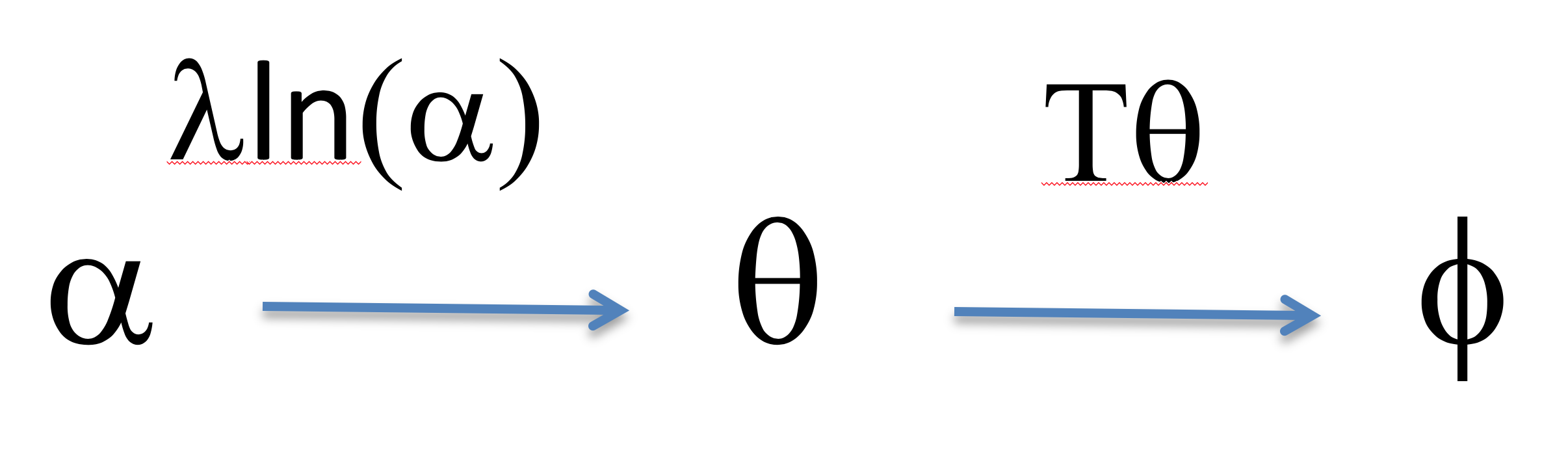
Figure 1: Transformations used in the phase-space. The original complex mode amplitudes $\bm{\alpha}$ are transformed first to constant-diffusion mode amplitudes $\bm{\theta}=\lambda\ln\left(\bm{\alpha}\right)$, then mapped with a possibly time-dependent mapping to real quadrature amplitudes $\bm{\phi}=\bm{T}\bm{\theta}$.

We now check that the traceless property persists after making this variable change to logarithmic variables. The Q-function is mapped to a set of constant diffusion, complex phase-space variables $\bm{\theta}$, as shown in Fig (1), which satisfy an equation of form:

$$\frac{\partial}{\partial t}Q^{\theta}=\mathcal{L}^{\theta}Q^{\theta}\,.$$ (48)

To prove the traceless property, a second mapping is made to a real quadrature vector, $\bm{\phi}=\left[\phi^{1},\ldots\phi^{2M}\right]$, described by the linear transformation $\bm{\phi}=\bm{T}\bm{\theta}.$ In this constant diffusion space, there are diagonal second derivative terms together with conjugate terms such that $D_{jj}^{\theta}=e^{-2i\eta_{j}}\left|D_{jj}^{\theta}\right|$, where $D_{jj}^{\theta}=i\lambda^{2}g_{jj}$. The corresponding real variables are defined in this case as:

$$\theta_{j}e^{i\eta_{j}}=x_{j}+iy_{j},$$ (49)

where $\bm{\phi}=\left(\bm{x},\bm{y}\right)$. For a one-mode case, the mapping transformation matrix from complex logarithmic to real variables is

$$\bm{T}=\left[\begin{array}[]{cc}e^{i\eta_{j}}&e^{-i\eta_{j}}\\ -ie^{i\eta_{j}}&ie^{-i\eta_{j}}\end{array}\right].$$ (50)

As a result, the diagonal diffusion term in $\phi$ is

$$D^{jj}=-D^{j^{\prime}j^{\prime}}=\frac{1}{2}\left|D_{jj}^{\theta}\right|,$$ (51)

where $j^{\prime}=j+M$. There is a positive diffusion in $\bm{x}$ and negative diffusion in $\bm{y}$ as described in the previous subsection, except with a constant diffusion matrix.

The result is a transformed Q-function, $Q=Q^{\theta}\left|\delta\bm{\theta}/\delta\bm{\phi}\right|$, which evolves according to real differential equation. Introducing $\partial_{\mu}\equiv\partial/\partial\phi^{\mu}$, for $\mu=1,\ldots 2M$, the time-evolution equation is a TFPE with a diagonal, constant diffusion identical to Eq (44).

The transformed diffusion matrix is traceless as shown previously, so that $\sum D^{\mu\mu}=0\,.$ The phase-space probability $Q$ is positive, yet since the overall diffusion term $\bm{D}$ is not positive definite, this is not a forward-time stochastic process [77]. The form of Eq (44) means that probability is conserved by the dynamical equations, provided boundary terms vanish, which is also required from the definition and Eq (3), so that for a $2M$-dimensional real measure $d\bm{\phi}$:

$$\int d\bm{\phi}Q\left(\bm{\phi},t\right)=1\,.$$ (52)

The Q-function obeys a second order partial differential equation. Yet it describes a reversible process. Positive distribution functions in statistical mechanics commonly follow a diffusion equation which is irreversible, owing to couplings to a reservoir. Since the Q-function is a phase-space representation that is positive, it can be treated and sampled in a similar way to a probability distribution.

III Time-symmetric stochastic action

The Q-function for unitary evolution can be transformed to satisfy a real partial differential equation, with a traceless diffusion term that is not positive-definite. The resulting initial value problem is not well-posed unless the initial conditions have compact support in Fourier space [78]. Hence, Green’s functions with delta-function initial conditions [79] leading to a forward-time stochastic differential equation are not defined.

The alternative approach introduced here is to use Green’s functions with both initial and final boundary conditions for the TFPE, Eq (44). Our goal is to derive a quantum action principle [80] or path integral in Feynman’s terminology [38], with a real action integral. The leads to probabilistic evolution in space-time in which one can identify continuous sample trajectories.

The traceless property of the Q-function diffusion means that the phase space of $\bm{\phi}$ is generally divisible into two $M$-dimensional sub-vectors, so that $\bm{\phi}=\left[\bm{x},\bm{y}\right]$. These have the physical interpretation of complementary variables. The $\bm{x}$ fields will be called positive-time fields, with indices in the set $T_{+}$, while the $\bm{y}$ fields will be called negative-time fields, with indices in the set $T_{-}$, so that:

$$\bm{D} =\left[\begin{array}[]{cc}\bm{d}^{x}&\bm{0}\\ \bm{0}&-\bm{d}^{y}\end{array}\right],$$ (55)

$$\bm{A}\left(\bm{\phi}\right) =\left[\begin{array}[]{c}\bm{a}^{x}\left(\bm{\phi}\right)\\ -\bm{a}^{y}\left(\bm{\phi}\right)\end{array}\right].$$ (58)

The $\bm{d}^{x,y}$ matrices are assumed positive definite, where $d_{ij}^{x}=\left\{D^{ij}\right\}$ and $d_{ij}^{y}=\left\{-D^{i+M,j+M}\right\}$ for $i,j\leq M$. This is a more general scenario than a strictly diagonal diffusion, but includes it as a special case. Hence, there are two positive-definite differential operators, $\mathcal{L}^{x,y}$, such that $\mathcal{L}=\mathcal{L}^{x}-\mathcal{L}^{y}$, where:

$$\mathcal{L}^{x}= -\partial_{i}^{x}a_{i}^{x}\left(\bm{\phi}\right)+\frac{1}{2}\partial_{i}^{x}\partial_{j}^{x}d_{ij}^{x}$$

$$\mathcal{L}^{y}= -\partial_{i}^{y}a_{i}^{y}\left(\bm{\phi}\right)+\frac{1}{2}\partial_{i}^{y}\partial_{j}^{y}d_{ij}^{y}.$$ (59)

One usually solves for $Q\left(\bm{\phi},t\right)$ at a later time $t>t_{0}$, given an initial distribution $Q_{0}\left(\bm{\phi},t_{0}\right)$. However, not having positive-definite diffusion in $\bm{y}$ means that one cannot use standard Green’s functions or propagators to propagate $Q$ forward in time, without requiring singular Green’s functions. One also can’t propagate $Q$ purely backward in time, for the same reason.

III.1 Input and output boundary values

We will define time-symmetric propagators relative to combined boundary value conditions in the past and the future for the TFPE. We introduce a notation $P\left(\bm{\phi}_{OUT}\left|\bm{\phi}_{IN}\right.\right)$ to indicate the probability density of output event(s) $\bm{\phi}_{OUT}$ given input event(s) $\bm{\phi}_{IN}$. This does not imply time-ordering, and is different to the usage in quantum field theory [81] where time-ordering is implied. Both output and input events may include past and future times.

The input boundary coordinates will be labeled $\bm{\phi}_{IN}=\left(\bm{x}_{0},\bm{y}_{f}\right)$. This indicates a boundary at $t_{0}$ for positive-time fields $\bm{x}$, and at $t_{f}$ for negative-time fields $\bm{y}$. The complementary boundary $\bm{\phi}_{OUT}=\left(\bm{x}_{f},\bm{y}_{0}\right)$ is the output of the quantum process. As explained above, the terms input and output are used to indicate causality, not time-ordering. The joint probability of the input events in the past and future is defined as $P\left(\bm{\phi}_{IN},\bm{t}\right)$, where $\bm{t}=\left(t_{0},t_{f}\right)$ are the times involved.

Defining $d\bm{x}$ and $d\bm{y}$ as $M$-dimensional real measures, marginal distributions at the same time for $\bm{x}$ follow the usual conventions where:

$$P_{x}\left(\bm{x},t\right)=\int P\left(\bm{\phi},t\right)d\bm{y}\,,$$ (60)

andmarginal distributions for $\bm{y}$ are:

$$P_{y}\left(\bm{y},t\right)=\int P\left(\bm{\phi},t\right)d\bm{x}\,.$$ (61)

In some cases, the boundary values for the input distribution $P\left(\bm{\phi}_{IN},t\right)$ are independent of each other. This implies that one can write the joint probability of $\bm{x}_{0}$ in the past and and $\bm{y}_{f}$ in the future as a product of two independent distributions, so that

$$P\left(\bm{\phi}_{IN},\bm{t}\right)=P_{x}\left(\bm{x}_{0},t_{0}\right)P_{y}\left(\bm{y}_{f},t_{f}\right).$$ (62)

In general, there are correlations, and the boundary value distribution $P\left(\bm{\phi}_{IN},\bm{t}\right)$ cannot be factorized. This is the more general case that we analyze here. A graphical illustration of this is given in Fig (2). We use the convention that $P\left(\bm{\phi},t\right)$ is a general field probability, while $Q\left(\bm{\phi},t\right)$ is a probability in the restricted case which represents a quantum state.

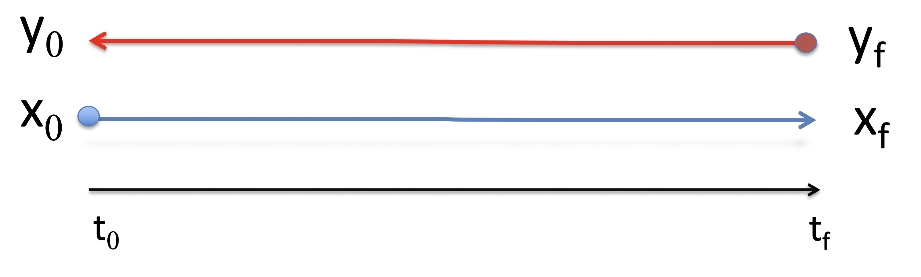
Figure 2: Quantum fields propagating in phase space, from initial time $t_{0}$ to final time $t_{f}$. The $\bm{x}$ components propagate in the positive time direction, while the $\bm{y}$ components propagate in the negative time direction. The joint probability of input events is $P\left(\bm{\phi}_{IN},\bm{t}\right)$, where $\bm{\phi}_{IN}=\left(\bm{x}_{0},\bm{y}_{f}\right)$.

III.2 Time-symmetric propagator

In contrast to the usual time-asymmetric propagator definitions [76], we now define a time-symmetric propagator (TSP). This is a function $G\left(\bm{\phi},t\left|\bm{\phi}_{IN},\bm{t}\right.\right)$, relative to inputs $\bm{\phi}_{IN}=\left[\bm{x}{}_{0},\bm{y}{}_{f}\right]$ and times $\bm{t}=\left[t_{0},t_{f}\right]$, where $t_{0}\leq t\leq t_{f}$. This is defined to satisfy the Q-function evolution equation with both initial and final delta-function boundary values:

$$\frac{\partial}{\partial t}G\left(\bm{\phi},t\left|\bm{\phi}_{IN},\bm{t}\right.\right)=\mathcal{L}G\left(\bm{\phi},t\left|\bm{\phi}_{IN},\bm{t}\right.\right).$$ (63)

Dropping the conditional arguments for brevity, the general equation of motion for the TSP is

$$\frac{dG\left(\bm{\phi},t\right)}{dt} =\left[-\partial_{\mu}A^{\mu}\left(\bm{\phi}\right)+\frac{1}{2}\partial_{\mu}\partial_{\nu}D^{\mu\nu}\left(\bm{\phi}\right)\right]G\left(\bm{\phi},t\right)$$

$$=\left[\mathcal{L}^{x}-\mathcal{L}^{y}\right]G\left(\bm{\phi},t\right),$$ (64)

with the property that $G\left(\bm{\phi},t\right)$ is positive and normalized so that

$$\int G\left(\bm{\phi},t\right)d\bm{\phi}=1.$$ (65)

The corresponding marginal distributions are given by:

$$G_{x}\left(\bm{x},t\left|\bm{\phi}_{IN},\bm{t}\right.\right) =\int d\bm{y}G\left(\bm{\phi},t\left|\bm{\phi}_{IN},\bm{t}\right.\right)$$

$$G_{y}\left(\bm{y},t\left|\bm{\phi}_{IN},\bm{t}\right.\right) =\int d\bm{x}G\left(\bm{\phi},t\left|\bm{\phi}_{IN},\bm{t}\right.\right).$$ (66)

The initial and final boundary conditions are delta-correlated marginal distributions, where $\delta\left(\bm{x}\right)$ is an $M-$dimensional real Dirac delta function, so that:

$$G_{x}\left(\bm{x},t_{0}\left|\bm{\phi}_{IN},\bm{t}\right.\right) =\delta\left(\bm{x}-\bm{x}{}_{0}\right)$$

$${G_{y}\left(\bm{y},t_{f}\left|\bm{\phi}_{IN},\bm{t}\right.\right)} {=\delta\left(\bm{y}-\bm{y}{}_{f}\right).}$$ (67)

This has the interpretation that, given input boundary values $\bm{\phi}_{IN}=\left[\bm{x}{}_{0},\bm{y}{}_{f}\right]$ at $t_{0},t_{f}$, the probability density of obtaining the field values $\bm{\phi}=\left[\bm{x},\bm{y}\right]$ at $t$ is $G\left(\bm{\phi},t\left|\bm{\phi}_{IN},\bm{t}\right.\right)$.

Since $\mathcal{L}$ is a linear operator, any linear combination or integral of propagators also satisfies the propagator time-evolution equation, (63). As a result, provided that $G\left(\bm{\phi},t_{0}\left|\bm{\phi}_{IN},\bm{t}\right.\right)$ can be integrated with respect to a nonlocal joint distribution $P\left(\bm{\phi}_{IN}\right)$ to obtain a Q-function at $t_{0}$, this gives a Q-function solution for all times:

$$Q\left(\bm{\phi},t\right)=\int d\bm{\phi}_{IN}G\left(\bm{\phi},t\left|\bm{\phi}_{IN},\bm{t}\right.\right)P\left(\bm{\phi}_{IN}\right)$$ (68)

When integrated over $\bm{x}_{f}$, $P\left(\bm{\phi}_{IN}\right)$ is a $Q$-function marginal distribution in $\bm{y}_{0}$ at time $t_{0}$, while if integrated $\bm{y}_{0}$ it is a $Q$-function marginal distribution in $\bm{x}_{f}$ at time $t_{f}$.

Having a nonlocal distribution $P\left(\bm{\phi}_{IN}\right)$ for the Q-function is not guaranteed in every case. A Q-function that is defined initially does not guarantee that $P\left(\bm{\phi}_{IN}\right)$ always exists. There may be Hamiltonians and states without any corresponding nonlocal distribution. In these cases we conjecture that one must define additional constraints or conditional boundaries, which are outside the scope of this paper.

III.3 Time-symmetric stochastic differential equation

To obtain a solution for the TSP, we introduce time-symmetric stochastic differential equations to define a set of stochastic paths. Subsequently, we will demonstrate that an integral over paths is a solution for the TSP, and satisfies the Q-function differential equation.

Time symmetric stochastic path equations are stochastic equations with both future and past boundary conditions [82]. These will be written in an intuitive form similar to a forward-backward stochastic differential equation [83]. The time-symmetric stochastic differential equation or TSSDE is defined to have the following structure, expressed as an integral:

$$\bm{x}(t) =\bm{x}_{0}+\int_{t_{0}}^{t}\bm{a}^{x}\left(\bm{\phi}\left(t^{\prime}\right)\right)dt^{\prime}+\int_{t_{0}}^{t}d\bm{w}^{x}$$

$$\bm{y}(t) =\bm{y}_{f}+\int_{t}^{t_{f}}\bm{a}^{y}\left(\bm{\phi}\left(t^{\prime}\right)\right)dt^{\prime}+\int_{t}^{t_{f}}d\bm{w}^{y}\,.$$ (69)

The two quadrature fields are propagated in the positive and negative time directions respectively, while the independent real Gaussian noise terms $d\bm{w}$ are correlated over short times so that, over a small interval $dt$:

$$\left\langle dw_{i}^{x}\left(t\right)dw_{j}^{x}\left(t\right)\right\rangle =d_{ij}^{x}dt\,$$

$$\left\langle dw_{i}^{y}\left(t\right)dw_{j}^{y}\left(t\right)\right\rangle =d_{ij}^{y}dt\,$$

$$\left\langle dw_{i}^{x}\left(t\right)dw_{j}^{y}\left(t\right)\right\rangle =0\,$$ (70)

These equations unify two important features: time symmetry and randomness. Similar equations occur in stochastic control theory, and there is literature on their properties [83], in a modified form. In our equations the boundary values in $\bm{x}_{0}$ and $\bm{y}_{f}$ are fixed rather than conditional on outputs. There is no third field as in some control theory equations. Analytic equations like this may be used to develop a stochastic perturbation theory [84] for quantum fields, and in some cases may have numerical iterative solutions.

While these provide insight into time symmetry, they clearly cannot be treated using conventional algorithms for ordinary stochastic differential equations. This can be recognized by attempting to write the equations as ordinary forward time stochastic differential equations. We may define $\bar{\bm{y}}\left(t\right)$ as a time-reversed copy of $\bm{y}\left(t\right)$, i.e., let $t_{-}=t_{0}+t_{f}-t$, and

$$\bar{\bm{y}}\left(t\right)=\text{{\hbox{\bm{y}\left(t_{-}\right)}}}\,.$$ (71)

The stochastic differential equation that results is:

$$d\bm{x} =\bm{a}^{x}\left(\bm{x}\left(t\right),\bar{\bm{y}}\left(t_{-}\right),t\right)dt+d\bm{w}^{x}$$

$$d\bar{\bm{y}} =-\bm{a}^{y}\left(\bm{x}\left(t_{-}\right),\bar{\bm{y}}\left(t\right),t_{-}\right)dt-d\bm{w}^{y}\,.$$ (72)

Here, $\bm{x}\left(t_{0}\right)=\bm{x}_{0}$ and $\bar{\bm{y}}\left(t_{0}\right)=\bm{y}_{f}$ are now “initial” conditions, but with the $y$ coordinate replaced by $\bar{y}$. A time-symmetric stochastic differential equation corresponds to stochastic propagation with drift terms having fields at different times. This non-locality in time prevents the direct use of standard local-time algorithms for solving the equations.

This behavior is not surprising, physically. If the fields had local drift terms, they would be causal theories that satisfy Bell’s theorem, which therefore do not correspond to quantum theory.

III.4 Discretized TSSDE

To analyze the stochastic equations, consider a time-symmetric stochastic trajectory discretized for times $t_{k}=t_{0}+k\epsilon$, with $k=0,\ldots n$, so that $t_{f}=t_{n}$ and $\bm{\phi}_{f}=\bm{\phi}_{n}$, where $\bm{\phi}_{k}\equiv\bm{\phi}\left(t_{k}\right)$. The notation $\bm{\phi}_{kj}\equiv\left(\bm{x}_{k},\bm{y}_{j}\right)$ is used for a field with quadratures at two different times. We now define an $n$-step path probability $\mathcal{G}\left(\left[\bm{\phi}\right]\left|\bm{\phi}_{0n}\right.\right)$ , where the input events are $\bm{\phi}_{IN}=\bm{\phi}_{0n}$.

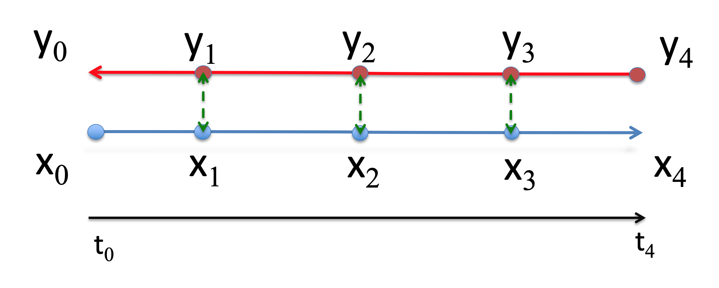
Figure 3: Quantum fields propagating over multiple time-intervals in phase space. Their interactions can lead to correlations. Coupling is indicated by green arrows.

Here ${\left[\bm{\phi}\right]=\left[\bm{\phi}_{0},\bm{\phi}_{1},\dots\bm{\phi}_{n-1},\bm{\phi}_{n}\right]}$, so this is the probability density of stochastic paths with points $\left[\bm{\phi}\right]$. This is shown diagrammatically in Fig (3 ). This type of path probability is always defined relative to specific time-symmetric inputs, $\bm{\phi}_{0n}\equiv\left(\bm{x}_{0},\bm{y}_{n}\right)$.

To simplify results with no loss of generality, we use orthogonal transformations and rescaling dilatations on $\bm{x}$ and $\bm{y}$, so that each diffusion matrix is diagonal: hence $\bm{d}^{x,y}=\bm{I}d$. The discretized equations are given by:

$$\bm{x}_{k} =\bm{x}_{k-1}+\bm{a}^{x}\left(\bm{\phi}_{k}^{\epsilon_{x}}\right)\epsilon+\bm{\Delta}_{k}^{x}$$

$$\bm{y}_{k-1} =\bm{y}_{k}+\bm{a}^{y}\left(\bm{\phi}_{k}^{\epsilon_{y}}\right)\epsilon+\bm{\Delta}_{k}^{y}.$$ (73)

These have Gaussian real noises $\bm{\Delta}_{k}^{x}$ such that, at each step in time,

$$\left\langle\Delta_{i}^{x}\Delta_{j}^{x}\right\rangle =\epsilon d\delta_{ij}$$

$$\left\langle\Delta_{i}^{y}\Delta_{j}^{y}\right\rangle =\epsilon d\delta_{ij}$$

$$\left\langle\Delta_{i}^{x}\Delta_{j}^{y}\right\rangle =0.$$ (74)

The time-symmetric SDE can be written in more than one equivalent discrete form. The discretized arguments of $\bm{a}^{x,y}$ generally are described by a $2\times 2$ matrix of coefficients $s_{zk}$, where $z=x,y$; $k=1,2$, and $0<s_{zk}<1$. These denote how the arguments of $\bm{a}^{x,y}$ are interpolated in terms of $\bm{\phi}_{k},\bm{\phi}_{k-1}$ . The general discretized form of the drift argument is $\bm{\phi}_{k}^{s}$, interpolated so that

$$\bm{\phi}_{k}^{s}=\left(s_{1}\bm{x}_{k-1}+\left(1-s_{1}\right)\bm{x}_{k},s_{2}\bm{y}_{k-1}+\left(1-s_{2}\right)\bm{y}_{k}\right).$$ (75)

These lead to equivalent discretized TSSDEs which all give the same stochastic process as $\delta\rightarrow 0$. However, they do not have the same path integral representations.

There are three particular types of TSSDE discretizations that are important here. These will be labelled forms I, II and III, depending on the way that the discretized arguments to the drift are calculated:

TSSDE I:

The $x$-arguments of $\bm{a}^{x,y}$ are evaluated at the earlier time, with $y$-arguments evaluated at the later time of each step, so $s_{z1}=1$, $s_{z2}=0$:

$${\bm{x}_{k}} {=\bm{x}_{k-1}+\bm{a}^{x}\left(\bm{\phi}_{k-1,k}\right)\epsilon+\bm{\Delta}_{k}^{x}}$$

$${\bm{y}_{k-1}} {=\bm{y}_{k}+\bm{a}^{y}\left(\bm{\phi}_{k-1,k}\right)\epsilon+\bm{\Delta}_{k}^{y}.}$$ (76)

This is an explicit equation, as the drift argument requires no knowledge of the solution for the next step for either variable. Such methods are similar to the Ito theory of ordinary stochastic differential equations [79].

TSSDE II:

Both arguments of $\bm{a}^{x,y}$ are evaluated at the beginning of each step in a forwards or backwards direction respectively, so $s_{xj}=1$, $s_{yj}=0$:

$${\bm{x}_{k}} {=\bm{x}_{k-1}+\bm{a}^{x}\left(\bm{\phi}_{k-1}\right)\epsilon+\bm{\Delta}_{k}^{x}}$$

$${\bm{y}_{k-1}} {=\bm{y}_{k}+\bm{a}^{y}\left(\bm{\phi}_{k}\right)\epsilon+\bm{\Delta}_{k}^{y}.}$$ (77)

This is a quasi-explicit equation, since the drift argument for $\bm{x}$ requires a knowledge of the next step for $\bm{y}$, and vice-versa. As a result, this has similar properties to type I.

TSSDE III:

In this fully symmetric form, the arguments of $\bm{a}^{x,y}$ are evaluated at the midpoint of each step, so $s_{zj}=\frac{1}{2}$. Defining $\bm{\bar{\phi}}_{k}=\left(\bm{\phi}_{k}+\bm{\phi}_{k-1}\right)/2$ gives:

$${\bm{x}_{k}} {=\bm{x}_{k-1}+\bm{a}^{x}\left(\bm{\bar{\phi}}_{k}\right)\epsilon+\bm{\Delta}_{k}^{x}}$$

$${\bm{y}_{k-1}} {=\bm{y}_{k}+\bm{a}^{y}\left(\bm{\bar{\phi}}_{k}\right)\epsilon+\bm{\Delta}_{k}^{y}.}$$ (78)

This is an implicit algorithm [85], as each drift argument requires knowledge of the solution for the next step in both variables.

Such techniques are often used to treat stochastic differential equations, as the equations follow standard calculus rules. This approach is similar to the Stratonovich theory of ordinary stochastic differential equations [26, 86, 79]. There are other discretizations possible as well, based on the general interpolation formula above.

III.5 Path integral and action

To obtain a path integral representation, we generalize methods used for forward stochastic differential equations [87]. The path probability density $\mathcal{G}\left(\left[\bm{\phi}\right]\left|\bm{\phi}_{0n},\left[\Delta\right]\right.\right)$ is conditioned both on an input $\bm{\phi}_{0n}$ and a random noise vector, $\left[\bm{\Delta}\right]=\bm{\Delta}_{1}^{x},\bm{\Delta}_{1}^{y},\ldots\bm{\Delta}_{n}^{x},\bm{\Delta}_{n}^{y}$, where $\bm{\Delta}_{j}=\left(\bm{\Delta}_{j}^{x},\bm{\Delta}_{j}^{y}\right)$ are independent $2M-$dimensional real Gaussian noises. This conditional path probability is a product of Dirac delta functions, since only one path exists for a given initial condition and noise sample:

$$\mathcal{G}_{n}\left(\left[\bm{\phi}\right]\left|\bm{\phi}_{0n},\left[\Delta\right]\right.\right) =\prod_{j=1}^{n}N_{j}\delta^{2M}\left(\epsilon\bm{v}_{j}-\bm{\Delta}_{j}\right).$$ (79)

Here we define relative velocity fields $\bm{v}=\left(\bm{v}_{j}^{x},\bm{v}_{j}^{y}\right)$ that correspond to a particular discretization, given above:

$$\bm{v}_{j}^{x} \equiv\frac{1}{\epsilon}\left(\bm{x}_{j}-\bm{x}_{j-1}\right)-\bm{a}^{x}\left(\bm{\phi}_{j}^{s_{x}}\right)$$

$$\bm{v}_{j}^{y} \equiv\frac{1}{\epsilon}\left(\bm{y}_{j-1}-\bm{y}_{j}\right)-\bm{a}^{y}\left(\bm{\phi}_{j}^{s_{y}}\right).$$ (80)

The normalization factor $N_{j}$ ensures that each term is normalized to unity when integrated over the output quadratures, which are $\bm{x}_{j}$ and $\bm{y}_{j-1}$ respectively. Since the delta-function can be written in the form of $\delta^{M}\left(\bm{x}_{j}-\bm{f}_{j}^{x}\right)\delta^{M}\left(\bm{y}_{j-1}-\bm{f}_{j}^{y}\right)$, the normalization includes derivatives of $\bm{f}_{j}^{x,y}$ . The simplest case is if the stochastic drift is defined explicitly using the input values of the quadrature field for that transition. This implies that $s_{x1}=1$ and $s_{y2}=0$, which includes TSSDE types I and II. For types I and II, we therefore have $N_{j}=1$.

Using delta-function integration identities, the general normalization is

$$N_{j}=N_{j}^{x}N_{j}^{y}=\prod_{k}\left(1-\epsilon\frac{\partial a^{xk}\left(\bm{\phi}_{j}^{s_{x}}\right)}{\partial x_{j}^{k}}\right)\left(1-\epsilon\frac{\partial a^{yk}\left(\bm{\phi}_{j}^{s_{y}}\right)}{\partial y_{j-1}^{k}}\right).$$ (81)

As a result, when there is an implicit drift, as in type III discretization, the normalization is modified.

Employing a Fourier transform representation of the delta function, where $d\bm{k}_{j}$ is a $2M$-dimensional real measure, this becomes:

$$\mathcal{G}\left(\left[\bm{\phi}\right]\left|\bm{\phi}_{0n},\left[\Delta\right]\right.\right) =\prod_{j=1}^{n}\int\frac{N_{j}d\bm{k}_{j}}{\left(2\pi\right)^{2M}}e^{-i\bm{k}_{j}\left(\bm{v}_{j}\delta-\bm{\Delta}_{j}\right)}.$$ (82)

For the $2M$ real Gaussian noises $\bm{\Delta}_{k}$, at each step in time, the probabilities of $\bm{\Delta}_{k}$ are:

$$P\left(\bm{\Delta}_{k}\right)=\frac{1}{\left(2\pi\epsilon d\right)^{M}}e^{-\left|\bm{\Delta}_{k}\right|^{2}/\left(2\epsilon d\right)}.$$ (83)

Hence the path probability conditioned on the inputs only can be written as a weighted integral over the step $\Delta$. This has the form, after $n$ steps, of a product of $n$ successive one-step path probabilities:

$$\mathcal{G}\left(\left[\bm{\phi}\right]\left|\bm{\phi}_{0n}\right.\right) =\prod_{j=1}^{n}\mathcal{G}\left(\bm{\phi}_{j-1},\bm{\phi}_{j}\right).$$ (84)

Here, $\mathcal{G}\left(\bm{\phi}_{j-1},\bm{\phi}_{j}\right)=\mathcal{G}_{j-1,j}$ is the probability of a one-step transition from $\bm{\phi}_{j-1,j}\rightarrow\bm{\phi}_{j,j-1},$ over the time interval $\epsilon$, which is:

$$\mathcal{G}_{j-1,j} =\int\frac{N_{j}d\bm{k}d\bm{\Delta}_{j}}{\left(\epsilon d\right)^{M}\left(2\pi\right)^{3M}}e^{-i\bm{k}\cdot\left(\bm{v}_{j}\epsilon-\bm{\Delta}_{j}\right)-\left|\bm{\Delta}_{j}\right|^{2}/\left(2\epsilon d\right)}.$$ (85)

This is integrated over $\bm{\Delta}_{j}$ by completing the square to give:

$$\mathcal{G}_{j-1,j} =\int\frac{N_{j}d\bm{k}}{\left(2\pi\right)^{2M}}e^{-\epsilon\left[d\left|\bm{k}\right|^{2}/2+i\bm{k}\cdot\bm{v}_{j}\right]}$$ (86)

Integrating over $\bm{k}$ gives an action principle for the path probability of the time-symmetric stochastic equation, in the form:

$$\mathcal{G}\left[\bm{\phi}\left|\bm{\phi}_{0n}\right.\right] =e^{-S_{0n}}.$$ (87)

The time-symmetric action from $t=t_{j}$ to $t=t_{n}$ is defined generally as

$${S_{jn}=\sum_{k=j+1}^{n}S_{k-1,k},}$$ (88)

where the one-step action for the $j$-th step is $S_{j-1,j}=S_{j-1,j}^{x}+S_{j-1,j}^{y}$, with

$$S_{j-1,j}^{x,y} =S^{x,y}\left(\bm{\phi}_{j-1},\bm{\phi}_{j}\right)$$

$$=\frac{\epsilon}{2d}\left|\bm{v}_{j}^{x,y}\right|^{2}+\ln\left(\sqrt{\mathcal{N}}/N_{j}^{x,y}\right),$$ (89)

The normalization factor is $\mathcal{N}=\left(2\pi\epsilon d\right)^{M}$. Both type I or type II discretizations have $N_{j}^{x,y}=1$, and reduce to the same continuous TSSDE.

The action is modified for type III discretization. This is a second order form where each drift term $\bar{\bm{a}}$ is evaluated at its midpoint value of $\bm{\bar{\phi}}_{k}=\left(\bm{\phi}_{k}+\bm{\phi}_{k-1}\right)/2$. Since this is an implicit discretization, the normalization of the delta-function 79 as a function of the output variables $\phi_{k,k-1}$ includes derivatives of the drift, $\bar{\bm{a}}$. Expanding the normalization factor $N_{j}$ in an exponential form, and including first-order terms in $\epsilon$, leads to a correction to the action [88]:

$$\bar{S}^{x,y}\left(\bm{\phi}_{k-1},\bm{\phi}_{k}\right) =\frac{\epsilon}{2}\left[\frac{1}{d}\left|\bar{\bm{v}}_{k}^{x,y}\right|^{2}+\nabla_{x,y}\bar{\bm{a}}_{k}^{x,y}\right]+\frac{\ln\mathcal{N}}{2},$$ (90)

where:

$$\bar{\bm{v}}_{k}^{x} \equiv\frac{\bm{x}_{k}-\bm{x}_{k-1}}{\epsilon}-\bm{a}^{x}\left(\bar{\bm{\phi}}_{k}\right)$$

$$\bar{\bm{v}}_{k}^{y} \equiv\frac{\bm{y}_{k-1}-\bm{y}_{k}}{\epsilon}-\bm{a}^{y}\left(\bar{\bm{\phi}}_{k}\right).$$ (91)

These results are for the constant diffusion case, and need modification if the diffusion depends on $\bm{\phi}.$

IV Q-function and path-integral

Next, we show that the integrated transition probability defined as a path integral gives a time-symmetric propagator, which therefore can generate a Q-function solution. This requires showing that the path integral form proposed for the TSP does satisfy the Q-function differential equation.

IV.1 TSP equivalence theorem:

The TSP, $G\left(\bm{\phi},t_{j}\left|\bm{\phi}_{0n},\bm{t}\right.\right)$, is obtained by integrating the $n$-step path probability $\mathcal{G}_{n}\left[\bm{\phi}\right]$ over all fields except $\bm{\phi}{}_{j}$ and the inputs $\bm{\phi}_{0n}$. Explicitly,

$$G\left(\bm{\phi},t_{j}\left|\bm{\phi}_{0n},\bm{t}\right.\right)=\int\mathcal{D}_{0n}\left[\bm{\phi}\right]\mathcal{G}\left[\bm{\phi}\left|\bm{\phi}_{0n}\right.\right]\delta\left(\bm{\phi}-\bm{\phi}_{j}\right),$$ (92)

where the lower indices on the path integral measure define the fixed endpoints:

$$\mathcal{D}_{0n}\left[\bm{\phi}\right]\equiv d\bm{y}_{0}d\bm{x}_{n}\prod_{k=1}^{n-1}d\bm{\phi}_{k}\,.$$ (93)

Corollary:

Provided the Q-function solution exists in integral form at initial time $t_{0}$, the solution at all times is an integrated path probability, multiplied by the joint probability of the input fields $\bm{\phi}_{0n}$:

$$Q\left(\bm{\phi},t_{j}\right)=\int\mathcal{D}\left[\bm{\phi}\right]\delta\left(\bm{\phi}-\bm{\phi}_{j}\right)\mathcal{G}_{n}\left[\bm{\phi}\right]P\left(\bm{\phi}_{0n}\right).$$ (94)

where the path integral measure is over all the coordinates

$$\mathcal{D}\left[\bm{\phi}\right]\equiv\prod_{k=0}^{n}d\bm{\phi}_{k}.$$ (95)

IV.1.1 Proof:

To demonstrate that integrating the conditional path probability $\mathcal{G}_{n}\left[\bm{\phi}\right]$ gives a time-symmetric propagator, requires showing that the propagator defined in (92) satisfies the time-evolution equation, (63), and has marginal delta-function boundaries in the past and future, (67).

General strategy:

This a generalization of earlier proofs of the equivalence between a path integral and a Fokker-Planck equation [88, 76]. Defining $G_{j}\left(\bm{\phi}\right)\equiv G\left(\bm{\phi},t_{j}\left|\bm{\phi}_{0n},\bm{t}\right.\right)$, and noting that $\mathcal{L}=\mathcal{L}^{x}-\mathcal{L}^{y}$,

$$G_{j+1}\left(\bm{\phi}\right)=\exp\left(\epsilon\mathcal{L}^{x}-\epsilon\mathcal{L}^{y}\right)G_{j}\left(\bm{\phi}\right)+O\left(\epsilon^{2}\right)\,.$$

It follows from the Baker-Haussdorf theorem that after discretization and taking the limit of small time-step $\epsilon$, the discrete form of the differential equation (64) can be written for $0\leq j<n$ as:

$$\left(1+\epsilon\mathcal{L}^{y}\right)G_{j+1}\left(\bm{\phi}\right)=\left(1+\epsilon\mathcal{L}^{x}\right)G_{j}\left(\bm{\phi}\right)+O\left(\epsilon^{2}\right)\,.$$ (96)

We will show that the postulated expansion in 92 for the TSP at time $t=t_{j}$ satisfies (96) to first order in $\delta$.

The path-integral expansions for the TSP at times $t=t_{j}$ and $t=t_{j+1}$ are

$$G_{j}\left(\bm{\phi}\right) =\int\mathcal{D}_{0n}\left[\bm{\phi}\right]e^{-S_{0n}}\delta\left(\bm{\phi}-\bm{\phi}_{j}\right)\,,$$

$$G_{j+1}\left(\bm{\phi}\right) =\int\mathcal{D}_{0n}\left[\bm{\phi}\right]e^{-S_{0n}}\delta\left(\bm{\phi}-\bm{\phi}_{j+1}\right)\,.$$ (97)

To prove (96), we introduce a hybrid probability for $\bm{\phi}_{j+1,j}\equiv\left(\bm{x}_{j+1},\bm{y}_{j}\right)$, defined as:

$$\bar{G}\left(\bm{\phi}\right) =\int\mathcal{D}_{on}\left[\bm{\phi}\right]e^{-S_{0n}}\delta\left(\bm{\phi}-\bm{\phi}_{j+1,j}\right).$$ (98)

and we will show in the following that in the limit of $\epsilon\rightarrow 0$,

$$\left(1+\epsilon\mathcal{L}^{y}\right)G_{j+1}\left(\bm{\phi}\right)=\left(1+\epsilon\mathcal{L}^{x}\right)G_{j}\left(\bm{\phi}\right) =\bar{G}\left(\bm{\phi}\right).$$ (99)

Boundary values:

First, we must prove that ,

$$G\left(\bm{\phi},t_{0}\left|\bm{\phi}_{0n},\bm{t}\right.\right) \propto\delta\left(\bm{x}-\bm{x}_{0}\right)$$

$$G\left(\bm{\phi},t_{n}\left|\bm{\phi}_{0n},\bm{t}\right.\right) \propto\delta\left(\bm{y}-\bm{y}_{n}\right).$$ (100)

However, the existence of delta-function boundary values is immediate. From (92), since $D_{0n}\left[\bm{\phi}\right]$ has no measure including $\bm{x}_{0}$, it follows immediately that:

$$G\left(\bm{\phi},t_{0}\left|\bm{\phi}_{0n},\bm{t}\right.\right) =\int\mathcal{D}_{0n}\left[\bm{\phi}\right]\mathcal{G}_{n}\left[\bm{\phi}\right]\delta\left(\bm{\phi}-\bm{\phi}_{0}\right)$$ (101)

$$=\delta\left(\bm{x}-\bm{x}_{0}\right)\int\mathcal{D}_{0n}\left[\bm{\phi}\right]\mathcal{G}_{n}\left[\bm{\phi}\right]\delta\left(\bm{y}-\bm{y}_{0}\right).$$

Similarly, since $D_{0n}\left[\bm{\phi}\right]$ has no measure including $\bm{y}_{n}$,

$$G\left(\bm{\phi},t_{n}\left|\bm{\phi}_{0n},\bm{t}\right.\right)=\delta\left(\bm{y}-\bm{y}_{n}\right)\int\mathcal{D}_{0n}\left[\bm{\phi}\right]\mathcal{G}_{n}\left[\bm{\phi}\right]\delta\left(\bm{x}-\bm{x}_{n}\right).$$

Single-step probability identity:

We next prove a differential identity for the single-step transition probability in $\bm{x}$, which factorizes from the transition probability in $\bm{y}$ at short times. As $\epsilon\rightarrow 0$, using the Fourier representation of the step probability in Eq (86), the single step transition probability in $\bm{x}$ is:

$$e^{-S_{j,j+1}^{x}}=\int\frac{d\bm{k}^{x}}{\left(2\pi\right)^{M}}e^{-\epsilon\left[d\left|\bm{k}^{x}\right|^{2}/2+i\bm{k}^{x}\cdot\bm{v}_{j+1}^{x}\right]}.$$ (102)

Recalling the definition of relative velocity in Eq (80), we use a type II discretization, and define the drift for $S_{j,j+1}^{x}$ as

$$\bm{a}_{j}^{x} \equiv\bm{a}^{x}\left(\bm{\phi}_{j}\right)$$

$$\bm{a}_{j}^{y} \equiv\bm{a}^{y}\left(\bm{\phi}_{j+1}\right).$$ (103)

As a result, this can be written as:

$$e^{-S_{j,j+1}^{x}} =\int\frac{d\bm{k}^{x}}{\left(2\pi\right)^{M}}e^{-\epsilon\left(\frac{d}{2}\left|\bm{k}^{x}\right|^{2}-i\bm{k}^{x}\cdot\bm{a}_{j}^{x}\right)-i\bm{k}^{x}\cdot\left(\bm{x}_{j+1}-\bm{x}_{j}\right)}.$$ (104)

Expanding to first order in $\epsilon,$ and taking derivatives of the exponential with respect to $\bm{x}_{j}$, gives the identity that:

$$e^{-S_{j,j+1}^{x}} =\left[1+\epsilon\tilde{\mathcal{L}}_{j}^{x}\right]\int\frac{d\bm{k}^{x}}{\left(2\pi\right)^{M}}e^{-i\bm{k}^{x}\cdot\left(\bm{x}_{j+1}-\bm{x}_{j}\right)}.$$ (105)

where $\mathcal{\tilde{L}}_{j}^{x}$ is the adjoint of the differential operator $\mathcal{L}^{x}$ evaluated at $x_{j}$:

$$\tilde{\mathcal{L}}_{j}^{x}\equiv\frac{d}{2}\nabla_{x_{j}}^{2}+\bm{a}_{j}^{x}\cdot\bm{\nabla}_{x_{j}}.$$ (106)

Equivalently, on carrying out the inverse Fourier transform,

$$e^{-S_{j,j+1}^{x}}=\left[1+\epsilon\tilde{\mathcal{L}}_{j}^{x}\right]\delta\left(\bm{x}_{j}-\bm{x}_{j+1}\right)+O\left(\epsilon^{2}\right).$$

Hybrid probability:

Inserting this expression into the expansion of the hybrid probability, (98), and integrating twice by parts (assuming vanishing probability at the phase-space boundaries), leads to

$$\bar{G}\left(\bm{\phi}\right) =\int\mathcal{D}_{on}\left[\bm{\phi}\right]\delta\left(\bm{x}_{j}-\bm{x}_{j+1}\right)\delta\left(\bm{\phi}-\bm{\phi}_{j+1,j}\right)$$

$$\,\,\,\times\left[1+\epsilon\mathcal{L}_{j}^{x}\right]e^{-S_{0n}^{y}-S_{0j}^{x}-S_{j+1,n}^{x}}.$$ (107)

where:

$$\mathcal{L}_{j}^{x}\equiv\frac{d}{2}\nabla_{x_{j}}^{2}-\bm{\nabla}_{x_{j}}\cdot\bm{a}_{j}^{x}.$$ (108)

On integration over $\bm{x}_{j}$, using the delta-function in $\bm{x}_{j}$, all terms in the path integral involving $\bm{x}_{j}$ can be replaced by $\bm{x}_{j+1}$. The $\bm{x}$ coordinates are now relabeled so that $\bm{x}^{\prime}_{k}=\bm{x}{}_{k}$ for $k<j$ and $\bm{x}^{\prime}_{k-1}=\bm{x}{}_{k}$ for $k>j$ . As a result of the second delta-function in $\bm{x}$, inside the integral $\bm{x}_{j+1}\equiv\bm{x}_{j}^{\prime}=\bm{x}$, so that

$$\bar{G}\left(\bm{\phi}\right) =\left[1+\epsilon\mathcal{L}^{x}\right]\int\mathcal{N}^{n}\left(\prod_{k=1}^{n-1}d\bm{x}_{k}^{\prime}\right)\left(\prod_{k=0}^{n-1}d\bm{y}_{k}\right)\,$$

$$\,\,\,\times\delta\left(\bm{\phi}-\bm{\phi}_{j}^{\prime}\right)e^{-S_{0,n}^{\prime y}-S_{0,n-1}^{\prime x}}.$$ (109)

This has a contracted time path in $\bm{x}$, since one of the $\bm{x}$ integrals and its corresponding propagator is now removed.

Hybrid discretization:

Here, $\bm{\phi}_{k}^{\prime}\equiv\left(\bm{x}_{k}^{\prime},\bm{y}_{k}\right),$ and a corresponding action for $S_{k,k+1}^{\prime x}$ is defined with a drift in $x$, $y$ that is as previously for $k<j$. For $k\geq j$ one now has a type I discretization, since:

$$\bm{a}_{k}^{\prime x} =\bm{a}_{k+1}^{x}=\bm{a}^{x}\left(\bm{x}_{k}^{\prime},\bm{y}_{k+1}\right)$$

$$\bm{a}_{k}^{\prime y} =\bm{a}_{k}^{y}=\bm{a}^{x}\left(\bm{x}_{k}^{\prime},\bm{y}_{k+1}\right).$$ (110)

This means that the hybrid propagator has a hybrid discretization, part type I and part type II, with

$$S_{k-1,k}^{\prime}=\frac{\epsilon}{2}\left[\bm{v}_{k}^{\prime T}\left(\bm{d}^{x}\right)^{-1}\bm{v}_{k}^{\prime}\right]+\ln\mathcal{N}.$$ (111)

To keep the total number of integration variables the same, a new output variable $\bm{x}^{\prime}_{n}$ at $t=t_{n}$ is added to the integration measure, with a corresponding action. The new drift terms are independent of $\bm{x}^{\prime}_{n}$, as the modified action is a type I action, since $n\geq j$.

The corresponding integration weighted by $S_{n-1,n}^{x\prime}$ is normalized, and equals unity. Hence, adding the new variable and integration leaves $\bar{G}\left(\bm{\phi}\right)$ invariant. Since type I and type II discretizations are identical in the limit of $\epsilon\rightarrow 0$, we therefore have proved that:

$$\bar{G}\left(\bm{\phi}\right)=\left[1+\epsilon\mathcal{L}^{x}\right]G_{j}\left(\bm{\phi}\right)\,.$$ (112)

Next, carrying out the complementary procedure for the $\bm{y}$ variable, we obtain a contraction in the number of $\bm{y}$ variables, with a new variable added called $\bm{y}_{0}^{\prime}$. This also has a type I action, and integrates to unity. The calculation is a mirror image of the one above, leading to the required result:

$$\bar{G}\left(\bm{\phi}\right)=\left[1+\epsilon\mathcal{L}^{y}\right]G_{j+1}\left(\bm{\phi}\right)\,.$$ (113)

This proves the required differential identity.

IV.2 Time-symmetric quantum action principle

The results above show that the probability density for quantum time-evolution is given by a path integral over a real Lagrangian, where in each small time interval the propagators factorize. These equations can be solved using path integrals over both the propagators.

The path then no longer has to be over an infinitesimal distance in time, and the total propagators will not factorize. This is a type of stochastic bridge [7, 8, 9], which acts in two time directions simultaneously. The action functional $S$ is an integral over an effective Lagrangian, which is equivalent to a discrete sum in the limit of small time-steps:

$$\lim_{\epsilon\rightarrow 0}S\left[\bm{\phi}\right]=\int_{t_{0}}^{t_{f}}L\left(\bm{\phi},\dot{\bm{\phi}}\right)dt+n\ln\mathcal{N},$$ (114)

with a number of steps $n$ inverse to the step-size, so that $n\equiv\left(t_{f}-t_{0}\right)/\epsilon$. We note that the stochastic equation probabilities are independent of the type of discretization, so any discretization is possible. This continuum limit is most readily obtained for the symmetric type III discretization, which is known to reach a continuum limit uniformly for forward-time path integrals [89, 90, 91], allowing the use of standard calculus.

In order to write the action in a unified form, we define a combined, central difference Lagrangian as

$$L=L^{x}(\bm{\phi},\dot{\bm{\phi}})+L^{y}(\bm{\phi},-\dot{\bm{\phi}})\,,$$ (115)

so that the action integral can be written in the positive time direction for $t_{0}<t<t_{f}$, with a total Lagrangian of

$$L =\sum_{\mu}\frac{1}{2d}\left(\dot{\phi}^{\mu}-A^{\mu}\left(\bm{\phi},t\right)\right)^{2}-V\left(\bm{\phi}\right).$$ (116)

Here the potential term $V$ includes contributions of opposite sign from the positive and negative time fields, so that

$$V\left(\bm{\phi},t\right)=-\frac{1}{2}\sum_{\mu}\partial_{\mu}a^{\mu}\left(\bm{\phi}\right).$$ (117)

This defines the total probability for an $n$-step open stochastic bidirectional bridge, with constant diffusion, central difference evaluation of the action, and fixed intermediate points:

$$G\left(\left[\bm{\phi}\right]\left|\bm{\phi}_{IN}\right.\right)=\mathcal{N}^{n}e^{-\int_{t_{0}}^{t_{f}}L(\bm{\phi},\dot{\bm{\phi}})dt}.$$ (118)

On integrating over the intermediate points, with drift terms defined at the center of each step in phase-space, this can be written in a notation analogous to a quantum-mechanical transition amplitude in a Feynman path integral. One obtains the Q-function in this limit as:

$$Q\left(\bm{\phi}^{\prime},t^{\prime}\right)=\int d\mu\left[\bm{\phi}\right]\delta\left(\bm{\phi}\left(t^{\prime}\right)-\bm{\phi}^{\prime}\right)e^{-\int_{t_{0}}^{t_{f}}L(\bm{\phi},\dot{\bm{\phi}})dt^{\prime}}P\left(\bm{\phi}_{IN}\right)$$

where $t_{n}=t_{0}+n\epsilon$, and we integrate over all phase-space points with a normalized measure:

$$d\mu\left[\bm{\phi}\right]=\lim_{\epsilon\rightarrow 0}\mathcal{N}^{n}\prod_{k=0}^{n}d\bm{\phi}_{k}\,.$$ (119)

The paths $\bm{\phi}\left(t\right)$ are defined so that $\bm{\phi}_{IN}=\left(\bm{x}_{0},\bm{y}_{f}\right)$, where $\bm{x}\left(t_{0}\right)=\bm{x}_{0}$ and $\bm{y}\left(t_{n}\right)=\bm{y}_{f}$ are defined at the initial and final times respectively.

V Extra dimensions

Many techniques exist for evaluating real path-integrals, both numerical and analytic. There is a formal analogy between the form given above and the expression for a Euclidean path integral of a polymer, or a charged particle in a magnetic field. Here we obtain an extra-dimensional technique for probabilistic sampling of the time-symmetric path integral, which also gives an algorithm for evaluating the solution to a TSSDE. Similar results are known for forward time stochastic equations [8, 9].

V.1 Equilibration in higher dimensions

To make use of the real path-integral, one needs to probabilistically sample the entire space-time path, since each part of the path depends in general on other parts. To achieve this, we add an additional ’virtual’ time dimension, $\tau$. This is used in the related statistical problem of stochastic bridges, for computing a stochastic trajectory that is constrained by a future boundary condition [7, 92, 8, 93, 9].

This extra-dimensional functional distribution, $\mathcal{P}\left([\bm{\phi}],\tau\right)$, is defined so that the probability tends asymptotically for large $\tau$ to the required solution:

$$\lim_{\tau\rightarrow\infty}\mathcal{P}\left([\bm{\phi}],\tau\right)=\mathcal{G}\left(\left[\bm{\phi}\right]\left|\bm{\phi}_{IN}\right.\right)\,.$$ (120)

The solution is such that $\bm{\phi}\left(t\right)$ is constrained so that $\bm{x}\left(t_{0}\right)=\bm{x}_{0}$ , and $\bm{y}\left(t_{f}\right)=\bm{y}_{f}$, where $\bm{x}_{0},\bm{y}_{f}$ are randomly distributed as $\mathcal{P}\left(\bm{x}_{0},\bm{y}_{f}\right)$ for the case of an nonlocal input boundary. We use the Type III midpoint form of the Lagrangian.

It has been shown in work on stochastic bridges [8] that sampling using a stochastic partial differential equation (SPDE) can be applied to cases where one of the boundary conditions is free. To define an SPDE the other boundary condition on $\bm{x}$ is specified so that $\dot{\bm{x}}\left(t_{f}\right)=\bm{a}^{x}\left(\bm{\phi}\left(t_{f}\right)\right)$, with a boundary condition for $\dot{\bm{y}}$ so that $\dot{\bm{y}}\left(t_{0}\right)=-\bm{a}^{y}\left(\bm{\phi}\left(t_{0}\right)\right)$.

This is consistent with the open boundary conditions of the path integral in real time, since in the limit of $\epsilon\rightarrow 0$, the path integral weight implies that one must have $\dot{\bm{x}}\left(t_{f}\right)=\bm{a}^{x}\left(\bm{\phi}\left(t_{f}\right)\right)+O\left(\sqrt{\epsilon}\right)$ and $\dot{\bm{y}}\left(t_{0}\right)=-\bm{a}^{y}\left(\bm{\phi}\left(t_{0}\right)\right)+O\left(\sqrt{\epsilon}\right)$. The effect of the additional terms proportional to $\sqrt{\epsilon}$ vanish as $\epsilon\rightarrow 0$, as they contributes a negligible change to the entire path integral. This open boundary condition is necessary in order to have a well-defined partial differential equation in higher dimensions.

Extra-dimensional equilibration is seldom used for conventional SDE sampling, as direct evolution is more efficient. However, we will show that SPDE sampling is applicable to time-symmetric propagation, where direct sampling is not possible without additional iteration. In this section, a simplification is made by rescaling the variables to make the diffusion $d^{\mu}\left(t\right)$ independent of time and index, i.e., $d^{\mu}\left(t\right)=d$, as in the previous section.

The SPDE is obtained as follows [9]. Firstly suppose that $\mathcal{P}\left([\bm{\phi}],\tau\right)$ satisfies a functional partial differential equation of

$$\frac{\partial\mathcal{P}}{\partial\tau}=\int_{t_{0}}^{t_{f}}dt\sum_{\mu}\frac{\delta}{\delta\phi^{\mu}(t)}\left[-\mathcal{A}^{\mu}\left(\bm{\phi},t\right)+d\frac{\delta}{\delta\phi^{\mu}(t)}\right]\mathcal{P}\,.$$ (121)

In order that the asymptotic result agrees with the desired expression for $\mathcal{G}$, it follows from functional differentiation of Eq (84), that one must define $\bm{\mathcal{A}}\left(\bm{\phi},t\right)$ so that

$$\mathcal{A}^{\mu}\left(\bm{\phi},t\right)=-d\frac{\delta}{\delta\phi^{\mu}(t)}\int_{t_{0}}^{t_{f}}L(\bm{\phi},\dot{\bm{\phi}})dt^{\prime}.$$ (122)

This is a variational calculus problem, with one boundary fixed, and the other free. Variations vanish at the time boundaries where $\bm{\phi}$ is fixed. At the free boundaries, we choose that $\dot{\bm{\phi}}=\bm{A}$. In either case, boundary terms are zero because they occur in terms that vanish provided

$$\Delta\phi^{\nu}\frac{\partial L}{\partial\dot{\phi}^{\mu}}=\frac{\Delta\phi^{\nu}}{d}\left(\dot{\phi}^{\mu}-A^{\mu}\right)=0\,.$$ (123)

As a result, there are two type of natural boundary terms that allow partial integration to obtain Euler-Lagrange equations. Either one can set $\Delta\phi^{\mu}=0$ to give a fixed Dirichlet boundary term, or else one can set $\dot{\phi}^{\mu}=A^{\mu}$, to give an open Neumann boundary term. Hence, we choose to set $x^{j}=x_{0}^{j}$ and $\dot{y}^{j}=A^{yj}$ at $t=t_{0}$, while $y^{j}=y_{f}^{j}$ and $\dot{x}^{j}=A^{xj}$ at $t=t_{f}$. This allows one to obtain Euler-Lagrange type equations with an extra-dimensional drift defined as

$$\mathcal{A}^{\mu}\left(\bm{\phi},t\right) =d\left[\frac{d}{dt}\frac{\partial L}{\partial\dot{\phi}^{\mu}}-\frac{\partial L}{\partial\phi^{\mu}}\right]$$

$$=\frac{d}{dt}\left(\dot{\phi}^{\mu}-A^{\mu}\right)+\left(\dot{\phi}^{\nu}-A^{\nu}\right)\partial_{\mu}A^{\nu}+d\partial_{\mu}V\,.$$ (124)

The functional Fokker-Planck equation given above is then equivalent to a stochastic partial differential equation (SPDE):

$$\frac{\partial\bm{\phi}}{\partial\tau}=\bm{\mathcal{A}}\left(\bm{\phi},t\right)+\bm{\zeta}\left(t,\tau\right)\,,$$ (125)

where the stochastic term $\bm{\zeta}$ is a real delta-correlated Gaussian noise such that

$$\left\langle\zeta^{\mu}\left(t,\tau\right)\zeta^{\mu}\left(t^{\prime},\tau^{\prime}\right)\right\rangle=2d\delta^{\mu\nu}\delta\left(t-t^{\prime}\right)\delta\left(\tau-\tau^{\prime}\right).$$ (126)

V.2 Coefficients

Introducing first and second derivatives, $\dot{\bm{\phi}}\equiv\partial\bm{\phi}/\partial t$ and $\ddot{\bm{\phi}}\equiv\partial^{2}\bm{\phi}/\partial t^{2}$, there is an expansion for the higher-dimensional drift term $\bm{\mathcal{A}}$ in terms of the field time-derivatives:

$$\bm{\mathcal{A}}\left(\bm{\phi},t\right)=\ddot{\bm{\phi}}+\bm{C}\dot{\bm{\phi}}+\bm{U}\,.$$ (127)

Here, $\bm{C}$ is a circulation matrix that only exists when the usual potential conditions on the drift are not satisfied [9], while $\bm{U}$ is a pure drift without time-derivatives:

$$C^{\mu\nu} =\partial_{\mu}A^{\nu}-\partial_{\nu}A^{\mu}\,.$$ (128)

$$U^{\mu} =\partial_{\mu}\left(dV-\frac{1}{2}\sum_{\nu}\left(A^{\nu}\right)^{2}\right)\,.$$

The function $U$ acts to generate an effective force on the trajectories. The final stochastic partial differential equation that $\bm{\phi}$ must satisfy is therefore

$$\frac{\partial\bm{\phi}}{\partial\tau}=\ddot{\bm{\phi}}+\bm{C}\dot{\bm{\phi}}+\bm{U}+\bm{\zeta}\left(t,\tau\right)\,.$$ (129)

The final result is a c-number field stochastic partial differential equation in an extra space-time dimension, including an additional noise term. It has a steady-state that is equivalent to a full quantum evolution equation, and is identical to classical evolution in real time in the zero-noise limit, as shown in the next subsection.

The equations can be treated with standard techniques for stochastic partial differential equations [94]. The equations have $n_{d}+1$ dimensions in a manifold with $n_{d}$ space-time dimensions. The simplest case, for a single mode, has $n_{d}+1=2$ dimensions. In computational implementations, one can speed up convergence to the steady-state using Monte-Carlo acceleration [95].

V.3 Classical limit

The classical limit is for $d\rightarrow 0$. In this limit the higher-dimensional equations are noise-free and diffusive. Ignoring the noise term, one obtains:

$$\frac{\partial\phi^{\mu}}{\partial\tau}=\ddot{\phi}^{\mu}+\left[\partial_{\mu}A^{\nu}-\partial_{\nu}A^{\mu}\right]\dot{\phi}^{\nu}-A^{\nu}\partial_{\mu}A^{\nu}\,.$$ (130)

We wish to show that the classical trajectory solution, $\dot{\phi}^{\nu}=A^{\nu}$, is a possible steady-state solution. In this case, we obtain for these trajectories,

$$\frac{\partial\phi^{\mu}}{\partial\tau}=\frac{d}{dt}A^{\mu}-A^{\nu}\partial_{\nu}A^{\mu}.$$ (131)

Therefore, on a noise-free trajectory, the second derivative term simplifies to give

$$\frac{\partial\phi^{\mu}}{\partial\tau}=\left[\dot{\phi}^{\nu}-A^{\nu}\right]\partial_{\nu}A^{\mu}.$$

and hence for the classical trajectory one obtains

$$\frac{\partial\phi^{\mu}}{\partial\tau}=\mathcal{A}^{\mu}\left(\bm{\phi}\right)=0\,.$$ (132)

This extra-dimensional equation therefore has a steady state solution corresponding to the integrated classical field evolution in real time, namely:

$$\bm{x}(t) =\bm{x}(t_{0})+\int_{t_{0}}^{t}\bm{a}^{x}\left(\bm{\phi}\left(t^{\prime}\right)\right)dt^{\prime}$$

$$\bm{y}(t) =\bm{y}(t_{f})+\int_{t}^{t_{f}}\bm{a}^{y}\left(\bm{\phi}\left(t^{\prime}\right)\right)dt^{\prime}\,.$$ (133)

Both the initial and final boundary term equations are satisfied provided one chooses $\bm{x}\left(t_{0}\right)=\bm{x}_{0}$ and $\bm{y}\left(t_{f}\right)=\bm{y}_{f}$, if these are compatible, that is, if the dynamical equations have a solution. If one uses these equations to solve for $\bm{y}(t_{0})$, the solution can be rewritten in a more conventional form of a classical solution with initial conditions:

$$\bm{\phi}\left(t\right)=\bm{\phi}\left(t_{0}\right)+\int_{t_{0}}^{t}\bm{A}\left(\bm{\phi}\left(t^{\prime}\right)\right)dt^{\prime}.$$ (134)

The importance of imposing future-time boundary conditions in classical field problems like radiation-reaction has long been recognized in electrodynamics, including work by Dirac [1], as well as Wheeler and Feynman [12]. In such theories various field components typically require future-time restrictions on their dynamics. Hence the fact that future-time boundaries arise in the classical limit found here should not be very surprising.

Dirac [1] described his result that effectively gives a future boundary condition on electron acceleration in as “the most beautiful feature of the theory”. He explains: “We now have a striking departure from the usual ideas of mechanics. We must obtain solutions of our equations of motion for which the initial position and velocity of the electron are prescribed, together with its final acceleration, instead of solutions with all the initial conditions prescribed.”

If Dirac’s theory is compared with the classical limit obtained here, there are are clear similarities. His approach gave a dynamical condition required to derive the correct time evolution, using a restriction on the future boundaries of the radiation field. It is a striking feature of the present approach that Dirac’s idea of a future boundary condition arises naturally from the zero-noise limit of our equations.

V.4 Numerical methods

A variety of numerical techniques can be used to implement path integrals with a time-symmetric action. In this paper we solve the equivalent higher-dimensional partial stochastic differential equation with a finite difference implementation. This permits Neumann, Dirichlet and other boundary conditions to be imposed. We also explain strategies for dealing with future time boundaries, which is the most obvious practical issue with this approach.

V.4.1 SPDE integration

First, we demonstrate convergence of the higher dimensional method, for an ordinary stochastic differential equation. We use a central difference implicit method that iterates to obtain convergence at each step, including an iteration of the boundary conditions. The method is similar to a central difference method described elsewhere [85, 94]. A simple finite difference implementation of the Laplacian is used to implement non-periodic time boundaries.

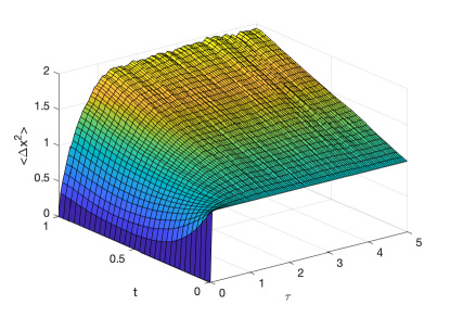
Figure 4: Example of SPDE solution with an extra dimension. The component $x$ propagates in the positive time direction as a random Wiener process. The expected variance for $\tau\rightarrow\infty$ is $\left\langle x^{2}\left(t,\tau\right)\right\rangle=1+t$, with $\left\langle x^{2}\left(0,\tau\right)\right\rangle=1$. Fluctuations are sampling errors due to a finite number of $10000$ trajectories. Variance error bars due to sampling errors were estimated as $\pm 2.5\%$, in good agreement with the difference between exact and simulated variance. A semi-implicit finite difference method [85, 96] was used to integrate the SPDE in $\tau$, with step-sizes of $\Delta\tau=0.0002$ and $\Delta t=0.03$. Errors from the finite step-size in $\tau$ were negligible. Finite differences were also used for the derivatives in $t$.

In order to demonstrate convergence, Fig (4) gives the computed numerical variance in an exactly soluble example of a stochastic differential equation with no drift term. We treat one variable with $\bm{C}=\bm{U}=0$, using a public-domain SPDE solver [97] with a random Gaussian initial condition of $\left\langle x_{0}^{2}\right\rangle=1$, where:

$$x(t)=x_{0}+\int_{0}^{t}dw_{x}\,.$$ (135)

This is a case of pure diffusion, so one expects the final equilibrium solution as $\tau\rightarrow\infty$ to be $\left\langle x^{2}\left(t,\tau\right)\right\rangle=1+t$. From Eq (129), the corresponding higher-dimensional stochastic process has boundary conditions of $x(t=0)=x_{0}$ and $\dot{x}(t=t_{f})=0$, while satisfying a stochastic partial differential equation:

$$\frac{\partial x}{\partial\tau}=\ddot{x}+\zeta\left(t,\tau\right)\,.$$ (136)

From the numerical results in Fig (4), the expected variance is reached uniformly in real time $t$ after pseudo-time $\tau\sim$ 2.5, to an excellent approximation, reaching $\left\langle x^{2}\right\rangle=1.95\pm 0.05$ at $t=t_{f}=1$ and $\tau=5$.

For the cases treated here, our focus is on accuracy rather than numerical efficiency. The purpose of the examples in this paper is to demonstrate how this approach works in simple cases. Checks were made to quantitatively estimate sampling error and step-size error in $\tau$. Substantial improvements in efficiency appear possible. It may be feasible to combine Ritz-Galerkin [98], spectral [94], or other methods [99] with boundary iteration. The MALA technique for accelerated convergence is also applicable [95].

VI Examples

Hamiltonians in quantum field theory of the type analyzed here have quadratic and quartic terms. In this section we consider two elementary examples, with details in single-mode cases. We consider a Hamiltonian of the form $\widehat{H}=\widehat{H}_{0}+\widehat{H}_{S}$. Here $\widehat{H}_{0}$ is a free field term, and $\widehat{H}_{S}$ describes quadrature squeezing, found in Hawking radiation or parametric down-conversion.Each of these cases will be treated separately below for simplicity, but they can be combined if required.

VI.1 Free-field case

After discretizing on a momentum lattice, and using the Einstein summation convention, the free-field Hamiltonian can be written in normally-ordered form as

$$\widehat{H}=\hbar\omega_{ij}\hat{a}_{i}^{\dagger}\hat{a}_{j}\,.$$ (137)

The corresponding Q-function equations are:

$$\dot{Q}^{\alpha}=-i\omega_{ij}\left[\frac{\partial}{\partial\alpha_{j}^{\ast}}\alpha_{i}^{\ast}-\frac{\partial}{\partial\alpha_{i}}\alpha_{j}\right]Q^{\alpha}\,.$$ (138)

Hence, the coherent amplitude evolution equations are:

$$\frac{d\alpha_{i}}{dt}=-i\omega_{ij}\alpha_{j}.$$ (139)

The simplest case is a single-mode simple harmonic oscillator Hamiltonian, such that: $\widehat{H}=\hbar\omega\hat{a}^{\dagger}\hat{a}\,.$ This corresponds to a characteristic equation of $\dot{\alpha}=-i\omega\alpha.$ The expectation value of the coherent amplitude in the Q-function has the equation:

$$\frac{\partial}{\partial t}\left\langle\alpha\right\rangle_{Q}=-i\omega\left\langle\alpha\right\rangle_{Q},$$ (140)

which is identical to the corresponding Heisenberg equation expectation value. There is no diffusive behavior or noise for these terms, and as a result the Q-function has an exactly soluble, deterministic quantum dynamics. The evolution is noise-free, with no need to make the transformations outlined above, since from (132), the steady-state in extra dimensions is given by solving(139). There is no difference between classical and quantum dynamics for coherent states, as pointed out by Schrödinger [100].

VI.2 Squeezed state evolution

Next, we consider quadratic interaction terms that are mapped to second-order derivatives in the Q-function. These cause squeezed state generation with quantum noise. They lead to a model for quantum measurement and quantum paradoxes [2].

Following the notation of Eq (28), the general squeezing interaction term is $\widehat{H}_{S}=\hbar\sum_{ij=0}^{M}\left[g_{ij00}\hat{a}_{i}^{\dagger}\hat{a}_{j}^{\dagger}+g_{00ij}\hat{a}_{i}\hat{a}_{j}\right]/2$. Such quadrature squeezing interactions are found in many areas of physics [71]. They illustrate how the Q-function equation behaves in the simplest nontrivial case where there is a diffusion term that is not positive-definite. We will investigate this in some detail, with numerical examples. This case illustrates how complementary variance changes are related to complementary time propagation directions.

Physically, these terms arise from parametric interactions, and lead to the dynamics that cause quantum entanglement. They are widespread, occurring in systems ranging from quantum optics to black holes, via Hawking radiation. The simplest case, with $g_{ij00}=\delta_{ij}$, is a single-mode quantum squeezing Hamiltonian:

$$\widehat{H}=\frac{i\hbar}{2}\left[\hat{a}^{\dagger 2}-h.c.\right]\,.$$ (141)

VI.2.1 Q-function dynamics

We can calculate directly how the Q-function evolves in time. Applying the correspondence rules as previously, one obtains a time-symmetric Fokker-Planck type equation, now with second-order terms. Combining these terms into one equation gives:

$$\frac{dQ^{\alpha}}{dt} =-\left[\frac{\partial}{\partial\alpha}\alpha^{\ast}+\frac{1}{2}\frac{\partial^{2}}{\partial\alpha^{2}}+h.c\right]Q^{\alpha}\,.$$ (142)

Using the standard quadrature definitions of Eq (40) one has $\alpha=q+ip$. The real phase space variables of Eq (49) with positive and negative diffusion are found by noting that $e^{i\eta}=i$, so making a variable change with $i\alpha=x+iy=iq-p$, we obtain

$$\frac{dQ}{dt}=\left[\partial_{x}x-\partial_{y}y+\frac{1}{4}\left(\partial_{x}^{2}-\partial_{y}^{2}\right)\right]Q\,.$$ (143)

This demonstrates the typical behavior of unitary Q-function equations. The diffusion matrix is traceless and equally divided into positive and negative definite parts. In this case the $x$ quadrature decays, but has positive diffusion, while the the $y$ quadrature shows growth and amplification, but has negative diffusion in the forward time direction. The amplified quadrature, which corresponds to the measured signal of a parametric amplifier, has a negative diffusion and is constrained by a future time boundary condition.

If initially factorizable, the $Q$-function solutions can always be factorized as a product with $Q=Q_{x}Q_{y}$. Then, if $t_{-}=t_{0}+t_{1}-t$, the time-evolution is diffusive, with an identical structure in each of two different time directions:

$$\frac{dQ_{y}}{dt_{-}} =\partial_{y}\left[-y+\frac{1}{4}\partial_{y}\right]Q_{y}$$

$$\frac{dQ_{x}}{dt} =\partial_{x}\left[-x+\frac{1}{4}\partial_{x}\right]Q_{x}\,.$$ (144)

The corresponding forward-backwards SDE is uncoupled, with decay and stochastic noise occurring in each time direction:

$$x(t) =x(t_{0})-\int_{t_{0}}^{t}x(t^{\prime})dt^{\prime}+\int_{t_{0}}^{t}dw_{x}$$

$$y(t) =y(t_{f})-\int_{t}^{t_{f}}y(t^{\prime})dt^{\prime}-\int_{t}^{t_{f}}dw_{y}\,.$$ (145)

where $\left\langle dw_{\mu}dw_{\nu}\right\rangle=\frac{1}{2}\delta_{\mu\nu}dt$. From these equations one can calculate immediately that

$$\frac{d}{dt}\left\langle x^{2}\right\rangle =2\left(\frac{1}{4}-\left\langle x^{2}\right\rangle\right)$$

$$\frac{d}{dt_{-}}\left\langle y^{2}\right\rangle =2\left(\frac{1}{4}-\left\langle y^{2}\right\rangle\right).$$ (146)

This equation for the variance time-evolution implies that the variance is therefore reduced in each quadrature’s intrinsic diffusion direction, for an initial vacuum state, with the solution in forward time given by

$$\left\langle x^{2}\left(t\right)\right\rangle =\frac{1}{4}\left(1+e^{-2t}\right)$$

$$\left\langle y^{2}\left(t\right)\right\rangle =\frac{1}{4}\left(1+e^{2t}\right).$$ (147)

Therefore, the variance reduction occurs in the forward time direction for $x$, giving rise to quadrature squeezing for an initial vacuum state, and in the backward time direction for $y$, leading to gain in the forward time direction. However, neither anti-normally ordered variance is reduced below $1/4$. This is the minimum possible, corresponding to zero variance in the unordered operator case.

With this choice of units, the diffusion coefficient is $d=1/2$, so the total Lagrangian of Eq (116) is:

$$L=\left(\dot{x}+x\right)^{2}+\left(\dot{y}-y\right)^{2}-1.$$ (148)

The net effect of the stochastic processes in opposite time directions is that growth in the uncertainty of one quadrature in one time direction is cancelled by the reduction in uncertainty of the other quadrature in the opposite time direction. This behavior is shown in Figs (5) to (9), which illustrate numerical solutions of the forward-backward equations using the techniques of the previous section.

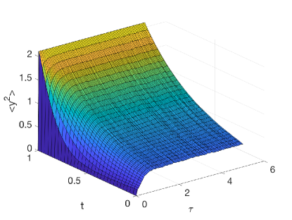
Figure 5: Variance of SPDE solution with an extra dimension. The unsqueezed quadrature $y$ propagates in the negative time direction, with boundaries fixed in the future. The extra-dimensional stochastic partial differential equation is solved out to $\tau=5$ , with a future time Dirichlet boundary at $t=1$ of a specified Gaussian distribution of $y$ with the correct variance at all $\tau$, and a past time Robin boundary at $t=0$ with a fixed derivative. Fluctuations are sampling errors due to a finite number of $6400$ stochastic trajectories. Other details as in Fig (4).

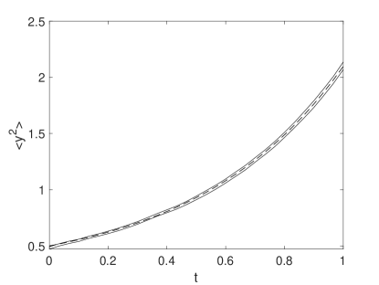
Figure 6: Example of SPDE solution with an extra dimension. The unsqueezed quadrature variance $y$ propagates in the negative time direction, with results obtained at virtual time $\tau=5$. The expected variance for $\tau\rightarrow\infty$ is $\left\langle y^{2}\left(t\right)\right\rangle=\frac{1}{4}\left(1+e^{2t}\right)$, and is shown as the dotted line. Fluctuations are sampling errors due to a finite number of $6400$ stochastic trajectories. The two solid lines are plus and minus one standard deviations from the mean. Other details as in Fig (4).

These solutions use 6400 trajectories, and hence include sampling error.

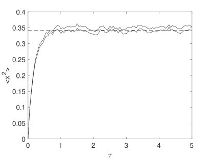
Figure 7: The equilibration in $\tau$ of the squeezed quadrature variance $x$ propagating in the positive time direction, with results obtained at real time $t=0.5$. Full equilibration is achieved for $\tau\gtrsim$1. Other details as in Fig (6).

Three dimensional graphs show equilibration in the extra dimension. Two dimensional graphs show results near equilibrium at $\tau=5$, with plots of variance in $x,y$ vs real time $t$ and virtual time $\tau$.

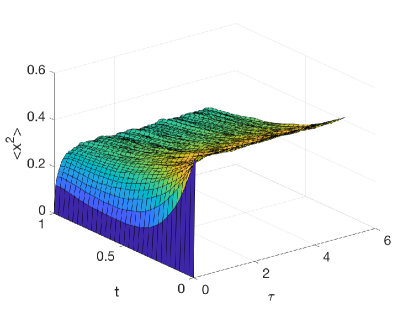
Figure 8: Variance of SPDE solution with an extra dimension. The squeezed quadrature $x$ propagates in the positive time direction, using a partial stochastic differential equation with with a past time Dirichlet boundary at $t=0$ of a specified Gaussian distribution in $x$ with the correct variance, and a future time Robin boundary at $t=1$ with a specified derivative. Other details as in Fig (6).

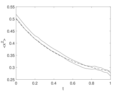
Figure 9: Example of SPDE solution with an extra dimension. The squeezed quadrature variance $x$, propagates in the positive time direction, with results obtained at virtual time $\tau=5$. The expected variance for $\tau\rightarrow\infty$ is $\left\langle x^{2}\left(t\right)\right\rangle=\frac{1}{4}\left(1+e^{-2t}\right)$, shown as the dotted line. Fluctuations are sampling errors due to a finite number of $1600$ stochastic trajectories. The two solid lines are plus and minus one standard deviations from the mean. Other details as in Fig (4).

VI.3 Comparison to operator equations

Defining quadrature operators $\hat{y}=\left(\hat{a}+\hat{a}^{\dagger}\right)/2=\hat{q}$ and $\hat{x}=i\left(\hat{a}-\hat{a}^{\dagger}\right)/2=-\hat{p}$, this physical system has the well-known behavior that the two variances change exponentially in time [101], in a complementary way. Given an initial vacuum state in which $\left\langle\hat{x}^{2}\left(0\right)\right\rangle=\left\langle\hat{y}^{2}\left(0\right)\right\rangle=1$, the Heisenberg equation solutions for the variances are

$$\left\langle\hat{x}^{2}\left(t\right)\right\rangle =\frac{1}{4}e^{-2t}$$

$$\left\langle\hat{y}^{2}\left(t\right)\right\rangle =\frac{1}{4}e^{2t}.$$ (149)

Hence, the $\hat{x}$ quadrature is squeezed, developing a variance below the vacuum fluctuation level, and the $\hat{y}$ quadrature is unsqueezed, developing a large variance. This maintains the Heisenberg uncertainty product, which is invariant.

Once operator ordering is taken into account, this gives an identical solution to the Q-function solution in Eq 147, because the operator correspondences are for anti-normal ordering. If we use $\{\}$ to denote anti-normal ordering, then

$$\left\langle\left\{\hat{x}^{2}\left(t\right)\right\}\right\rangle =\frac{1}{4}\left(1+e^{-2t}\right)$$

$$\left\langle\left\{y^{2}\left(t\right)\right\}\right\rangle =\frac{1}{4}\left(1+e^{2t}\right).$$ (150)

In both cases there is a reduction in variance in the direction of positive diffusion. If there is an initial vacuum state, then quadrature squeezing occurs in $x$ in the forward time direction, with a variance reduced below the vacuum level. Backward time squeezing occurs in $y$, which has forward-time gain.

VI.4 Higher dimensional stochastic equation

In the matrix notation used elsewhere, this means that we have $d=1/2$, and

$$\bm{A}=\left[\begin{array}[]{c}-x\\ y\end{array}\right],$$ (151)

with $\bm{c}=0$, so that the quantum dynamics occurs as the steady-state of a higher dimensional equation:

$$\frac{\partial\bm{\phi}}{\partial\tau}=\ddot{\bm{\phi}}-\bm{\phi}+\bm{\zeta}\left(t,\tau\right),$$ (152)

where $\left\langle\zeta^{\mu}\left(t,\tau\right)\zeta^{\nu}\left(t^{\prime},\tau^{\prime}\right)\right\rangle=\delta^{\mu\nu}\delta\left(\tau-\tau^{\prime}\right)\delta\left(t-t^{\prime}\right)$, with boundary values such that:

$$x\left(t_{0}\right) =x_{0}$$

$$y\left(t_{f}\right) =y_{f}$$

$$\dot{x}\left(t_{f}\right) =-x\left(t_{f}\right)$$

$$\dot{y}\left(t_{0}\right) =y\left(t_{0}\right)\,.$$ (153)

These are called mixed boundary conditions. They are partly Dirichlet (specified value), and partly Robin (specified linear combination of value and derivative). Numerical solutions for the the squeezed $x$ equations are given in Figs (8) and (9), while those for the unsqueezed $y$ equations are given in Figs (5) and (6). The effects of sampling error are seen through the two solid lines, giving one standard deviation variations from the mean. Exact results are included via the dashed lines.

VII Summary

The existence of a time-symmetric probabilistic action principle for quantum fields describes a different approach to the understanding of quantum dynamics. Neither imaginary time nor oscillatory path integrals are employed. More generally, time evolution through a symmetric stochastic action can be viewed as a dynamical principle in its own right. It is equivalent to the traditional action principle of quantum field theory. The advantage is that it is completely probabilistic, even for real-time quantum dynamics. Although not all commonly used Hamiltonians are included here, extensions to larger classes of quartic quantum field Hamiltonians appear feasible.

A property of this method is that it can provide an ontological interpretation of quantum mechanics. This quantum action principle can give a description of a reality that underlies the Copenhagen interpretation. The picture is of physical fields propagating both from the past to the future and from the future to the past. This time-symmetric interpretation, does not require a collapse of the wave-function. Such ontological interpretations are different to hidden variable theories [102], which only allow causality from past to future. As a result, one can have quantum features including vacuum fluctuations, sharp eigenvalues and even Bell violations [27], within a realistic and local framework.

The present paper has focused on the conceptual basis of this approach, and a proof of equivalence between quantum field dynamics and a time-symmetric stochastic action. The nonlocal boundary conditions used are different to local boundary conditions, and will not necessarily be equivalent to every quantum state, which are defined locally in time. Conditional boundaries are also possible in principle. These correspond to a larger set of possible Q-functions and Hamiltonians, but are outside the scope of the present paper.

The power of rapidly developing petascale and exascale computers appears well-suited to these approaches. Enlarged spatial lattices and increased parallelism are certainly needed. Yet this may not be as problematic to handle as either exponential complexity or the phase problems that arise in other approaches. It is intriguing that the utility of an extra dimension is widely recognized both in general relativity and quantum field theory. One may speculate that extending this action principle to curved space-time may yield novel quantum theories. This could lead to new approaches to unification.

References

• Dirac [1938] P. Dirac, Proc. R. Soc. London 167, 148 (1938).
• Drummond and Reid [2020] P. D. Drummond and M. D. Reid, Physical Review Research 2, 033266 (2020).
• Husimi [1940] K. Husimi, Proc. Physical Math. Soc. Jpn. 22, 264 (1940).
• Hillery et al. [1984] M. Hillery, R. F. O’Connell, M. O. Scully,  and E. P. Wigner, Phys. Rep. 106, 121 (1984).
• Drummond and Hillery [2014] P. D. Drummond and M. Hillery, The Quantum Theory of Nonlinear Optics (Cambridge University Press, 2014).
• Rosales-Zárate and Drummond [2015] L. E. C. Rosales-Zárate and P. D. Drummond, New Journal of Physics 17, 032002 (2015).
• Schrödinger [1931] E. Schrödinger, Sitzber Preuss. Akad. Wiss. Physik. Math. K1 , 144 (1931).
• Hairer et al. [2007] M. Hairer, A. M. Stuart,  and J. Voss, The Annals of Applied Probability 17, 1657 (2007).
• Drummond [2017] P. D. Drummond, Physical Review E 96, 042123 (2017).
• Reid [2017] M. Reid, Journal of Physics A: Mathematical and Theoretical 50, 41LT01 (2017).
• Tetrode [1922] H. M. Tetrode, Zeitschrift fur Physik 10, 317 (1922).
• Wheeler and Feynman [1945] J. A. Wheeler and R. P. Feynman, Reviews of Modern Physics 17, 157 (1945).
• Aharonov et al. [1964] Y. Aharonov, P. G. Bergmann,  and J. L. Lebowitz, Physical Review 134, B1410 (1964).
• Cramer [1980] J. G. Cramer, Phys. Rev. D 22, 362 (1980).
• Pegg [1982] D. T. Pegg, European Journal of Physics 3, 44 (1982).
• Pegg et al. [2002] D. T. Pegg, S. M. Barnett,  and J. Jeffers, Phys. Rev. A 66, 022106 (2002).
• Price [2008] H. Price, Studies in History and Philosophy of Science Part B: Studies in History and Philosophy of Modern Physics 39, 752 (2008).
• Argaman [2010] N. Argaman, American Journal of Physics 78, 1007 (2010).
• Fényes [1952] I. Fényes, Zeitschrift für Physik 132, 81 (1952).
• Nelson [1966] E. Nelson, Phys. Rev. 150, 1079 (1966).
• Grabert et al. [1979] H. Grabert, P. Hänggi,  and P. Talkner, Phys. Rev. A 19, 2440 (1979).
• Parisi et al. [1981] G. Parisi, Y. S. Wu, et al., Scientia Sinica 24, 483 (1981).
• Silver et al. [1990] R. N. Silver, D. S. Sivia,  and J. E. Gubernatis, Phys. Rev. B 41, 2380 (1990).
• Feldbrugge et al. [2017] J. Feldbrugge, J.-L. Lehners,  and N. Turok, Phys. Rev. D 95, 103508 (2017).
• Wiener [1930] N. Wiener, Acta mathematica 55, 117 (1930).
• Stratonovich [1966] R. Stratonovich, SIAM J. Control 4, 362 (1966).
• Drummond and Reid [2019] P. D. Drummond and M. D. Reid, arXiv preprint arXiv:1909.01798  (2019).
• Bernstein [1932] S. Bernstein, Verh. Internat. Math.-Kongr., Zurich , 288 (1932).
• Zambrini [1986] J. C. Zambrini, Physical review A 33, 1532 (1986).
• Kaluza [1921] T. Kaluza, Sitzungsber. Preuss. Akad. Wiss. Berlin.(Math. Physical) 1921, 966 (1921).
• Klein [1926] O. Klein, Zeitschrift für Physik 37, 895 (1926).
• Overduin and Wesson [1997] J. M. Overduin and P. S. Wesson, Physics Reports 283, 303 (1997).
• Horowitz [2005] G. T. Horowitz, New Journal of Physics 7, 201 (2005).
• Mohaupt [2003] T. Mohaupt, in Quantum gravity (Springer, 2003) pp. 173–251.
• Randall and Sundrum [1999] L. Randall and R. Sundrum, Phys. Rev. Lett. 83, 4690 (1999).
• Gogberashvili [2000] M. Gogberashvili, EPL (Europhysics Letters) 49, 396 (2000).
• Abbott [2006] E. A. Abbott, Flatland: A romance of many dimensions (OUP Oxford, 2006).
• Feynman et al. [2010] R. P. Feynman, A. R. Hibbs,  and D. F. Styer, Quantum mechanics and path integrals (Courier Corporation, 2010).
• Cosme et al. [2016] J. G. Cosme, C. Weiss,  and J. Brand, Phys. Rev. A 94, 043603 (2016).
• White [1992] S. R. White, Phys. Rev. Lett. 69, 2863 (1992).
• Drummond and Chaturvedi [2016] P. D. Drummond and S. Chaturvedi, Physica Scripta 91, 073007 (2016).
• Glauber [1963] R. J. Glauber, Phys. Rev. 131, 2766 (1963).
• Perelomov [1972] A. M. Perelomov, Comm. Math. Phys. 26, 222 (1972).
• Arecchi et al. [1972] F. T. Arecchi, E. Courtens, R. Gilmore,  and H. Thomas, Phys. Rev. A 6, 2211 (1972).
• Drummond [1984] P. D. Drummond, Phys. Letts. 106A, 118 (1984).
• Zambrini et al. [2003] R. Zambrini, S. M. Barnett, P. Colet,  and M. San Miguel, The European Physical Journal D-Atomic, Molecular, Optical and Plasma Physics 22, 461 (2003).
• Drummond and Gardiner [1980a] P. D. Drummond and C. W. Gardiner, J. Phys. A 13, 2353 (1980a).
• Drummond and Corney [1999] P. D. Drummond and J. F. Corney, Phys. Rev. A 60, R2661 (1999).
• Carter et al. [1987] S. J. Carter, P. D. Drummond, M. D. Reid,  and R. M. Shelby, Phys. Rev. Lett. 58, 1841 (1987).
• Deuar and Drummond [2007] P. Deuar and P. D. Drummond, Phys. Rev. Lett. 98, 120402 (2007).
• Corney et al. [2008] J. F. Corney, J. Heersink, R. Dong, V. Josse, P. D. Drummond, G. Leuchs,  and U. L. Andersen, Phys. Rev. A 78, 023831 (2008).
• Deuar and Drummond [2006a] P. Deuar and P. D. Drummond, J. Phys. A 39, 1163 (2006a).
• Deuar and Drummond [2006b] P. Deuar and P. D. Drummond, J. Phys. A 39, 2723 (2006b).
• Bargmann [1961] V. Bargmann, Commun. Pure Appl. Math. 14, 187 (1961).
• Steel et al. [1998] M. J. Steel, M. K. Olsen, L. I. Plimak, P. D. Drummond, S. M. Tan, M. J. Collett, D. F. Walls,  and R. Graham, Phys. Rev. A 58, 4824 (1998).
• Opanchuk and Drummond [2013] B. Opanchuk and P. D. Drummond, Journal of Mathematical Physics 54, 042107 (2013).
• Joseph et al. [2018a] R. R. Joseph, L. E. C. Rosales-Zárate,  and P. D. Drummond, Phys. Rev. A 98, 013638 (2018a).
• Joseph et al. [2018b] R. R. Joseph, L. E. Rosales-Zárate,  and P. D. Drummond, Journal of Physics A: Mathematical and Theoretical 51, 245302 (2018b).
• Balian and Brezin [1969] R. Balian and E. Brezin, Il Nuovo Cimento B 64, 37 (1969).
• Drummond and Gardiner [1980b] P. D. Drummond and C. W. Gardiner, Journal of Physics A: Math. Gen. 13, 2353 (1980b).
• Dirac [1945] P. A. M. Dirac, Rev. Mod. Phys. 17, 195 (1945).
• Cahill and Glauber [1969a] K. E. Cahill and R. J. Glauber, Phys. Rev. 177, 1857 (1969a).
• Cahill and Glauber [1969b] K. E. Cahill and R. J. Glauber, Phys. Rev. 177, 1882 (1969b).
• Corney and Drummond [2006a] J. F. Corney and P. D. Drummond, Journal of Physics A 39, 269 (2006a).
• Corney and Drummond [2006b] J. F. Corney and P. D. Drummond, Phys. Rev. B 73, 125112 (2006b).
• Arthurs and Kelly [1965] E. Arthurs and J. Kelly, The Bell System Technical Journal 44, 725 (1965).
• Leonhardt [1993] U. Leonhardt, Phys. Rev. A 48, 3265 (1993).
• Leonhardt and Paul [1993] U. Leonhardt and H. Paul, J. Mod. Optics 40, 1745 (1993).
• t’Hooft [1971] G. t’Hooft, Nuclear physics: B 33, 173 (1971).
• Corney and Drummond [2003] J. F. Corney and P. D. Drummond, Phys. Rev. A 68, 063822 (2003).
• Drummond and Ficek [2004] P. D. Drummond and Z. Ficek, eds., Quantum Squeezing (Springer-Verlag, Berlin, Heidelberg, New York, 2004).
• Milburn [1986] G. J. Milburn, Phys. Rev. A 33, 674 (1986).
• Altland and Haake [2012] A. Altland and F. Haake, Phys. Rev. Lett. 108, 073601 (2012).
• Drummond and Carter [1987] P. D. Drummond and S. J. Carter, J. Opt. Soc. Am. B 4, 1565 (1987).
• Zee [2010] A. Zee, Quantum field theory in a nutshell, Vol. 7 (Princeton university press, 2010).
• Graham [1977a] R. Graham, Zeitschrift für Physik B 26, 281 (1977a).
• Gardiner [1985a] C. W. Gardiner, Stochastic Methods, 1st ed. (Springer, Berlin, 1985).
• Miranker [1961] W. L. Miranker, Proceedings of the American Mathematical Society 12, 243 (1961).
• Gardiner [1985b] C. W. Gardiner, Handbook of Stochastic Methods, 2nd ed. (Springer-Verlag, Berlin, 1985) p. 442.
• Dirac [2005] P. A. Dirac, in Feynman’s Thesis: A New Approach To Quantum Theory (World Scientific, 2005) pp. 111–119.
• Weinberg [2015] S. Weinberg, Lectures on quantum mechanics (Cambridge University Press, 2015).
• Nualart and Pardoux [1991] D. Nualart and E. Pardoux, The Annals of Probability 19, 1118 (1991).
• Ma et al. [1994] J. Ma, P. Protter,  and J. Yong, Probability theory and related fields 98, 339 (1994).
• Chaturvedi and Drummond [1999] S. Chaturvedi and P. D. Drummond, Eur. Phys. J. B 8, 251 (1999).
• Drummond and Mortimer [1991a] P. Drummond and I. Mortimer, Journal of computational physics 93, 144 (1991a).
• Drummond and Mortimer [1991b] P. D. Drummond and I. K. Mortimer, J. Comput. Physical 93, 144 (1991b).
• Chow and Buice [2015] C. C. Chow and M. A. Buice, The Journal of Mathematical Neuroscience (JMN) 5, 8 (2015).
• Haken [1976] H. Haken, Zeitschrift für Physik B Condensed Matter 24, 321 (1976).
• Dekker [1978] H. Dekker, Physics Letters A 65, 388 (1978).
• Graham [1977b] R. Graham, Zeitschrift für Physik B 26, 397 (1977b).
• Graham [1977c] R. Graham, Phys. Rev. Lett. 38, 51 (1977c).
• Maier and Stein [1992] R. S. Maier and D. L. Stein, Phys. Rev. Lett. 69, 3691 (1992).
• Majumdar and Orland [2015] S. N. Majumdar and H. Orland, Journal of Statistical Mechanics: Theory and Experiment 2015, P06039 (2015).
• Werner and Drummond [1997a] M. J. Werner and P. D. Drummond, J. Comput. Phys. 132, 312 (1997a).
• Besag [1994] J. Besag, J. Roy. Statist. Soc. Ser. B 56, 591 (1994).
• Werner and Drummond [1997b] M. Werner and P. Drummond, Journal of Computational Physics 132, 312 (1997b).
• Kiesewetter et al. [2016] S. Kiesewetter, R. Polkinghorne, B. Opanchuk,  and P. D. Drummond, SoftwareX 5, 12 (2016).
• Matthies and Keese [2005] H. G. Matthies and A. Keese, Computer methods in applied mechanics and engineering 194, 1295 (2005).
• Keese [2003] A. Keese, Scientific Computing 6 (2003).
• Schrödinger [1926] E. Schrödinger, Naturwissenschaften 14, 664 (1926).
• Walls [1983] D. F. Walls, Nature 306, 141 (1983).
• Bell [1964] J. S. Bell, Physics 1, 195 (1964).