Demonstration of ThGEM-Multiwire Hybrid Charge Readout for Directional Dark Matter Searches

Abstract

Sensitivities of current directional dark matter search detectors using gas time projection chambers are now constrained by target mass. A ton-scale gas TPC detector will require large charge readout areas. We present a first demonstration of a novel ThGEM-Multiwire hybrid charge readout technology which combines the robust nature and high gas gain of Thick Gaseous Electron Multipliers with lower capacitive noise of a one-plane multiwire charge readout in SF₆ target gas. Measurements performed with this hybrid detector show an ion drift velocity of $138~{}\pm~{}10$ $\mathrm{m}\text{\,}{\mathrm{s}}^{-1}$ in a reduced drift field E/N of 93 $\times~{}10^{-17}$ $\mathrm{V}\text{\,}{\mathrm{cm}}^{2}$ with an effective gas gain of $2470\pm 160$ in 20 $\mathrm{Torr}$ of pure SF${}_{\text{6}}$ target gas.

1 Introduction

Detection and characterisation of dark matter (DM) - thought to be Weakly Interacting Massive Particles (WIMPs) [1, 2, 3] in a direction sensitive nuclear recoil detector with a suitable target material, is a major goal of the DM search community [4, 5, 6, 7]. This technology offers the potential to discriminate WIMP candidate events with galactic signature from terrestrial backgrounds/artefacts and hence, can probe below the so-called neutrino floor [8, 9, 10]. The use of low pressure gas Time Projection Chamber (TPC) technology, in which ionisation electrons from the nuclear recoil tracks are drifted to a charge readout plane and recorded for reconstruction, offers a route to achieving this goal. This is with potentials for low energy threshold and low background operations, including active electron recoil discrimination in the low WIMP mass parameter space.

The CYGNUS consortium is extensively exploring the feasibility of this technology for a large-scale experiment with aim to search for WIMPs beyond the so-called neutrino floor [4, 11]. This builds on previous R$\&$D and DM search results by multiple directional efforts, including DRIFT [12] , NEWAGE [13], MIMAC [14], D³ [15], DM-TPC [16] and CYGNO [17] collaborations. A feature of interest in DRIFT, for instance, is the use of CS₂ gas for primary ionization charge transport through negative ions (NI) drift, rather than drifting electrons for minimal and thermal scale diffusion [7, 18]. Primary ionization electrons from interactions in the TPC attach rapidly to the electronegative CS${}_{\text{2}}$ to form anions. These anions are drifted towards the readout plane where they are field ionized by the inhomogeneous high electric field in this region - thereby inducing signal amplification by electron avalanche [18]. The use of NI drift substantially reduces blurring of the tracks by diffusion [18, 19, 20], and hence saves cost by allowing the possibility for longer drift distances relative to the conventional electron drift concepts.

Recently, it has been discovered that SF₆ [21, 22], which has lower toxicity with improved handling over CS₂ [23], can also serve as a negative ion TPC gas. This is with a further advantage of formation of a minority charge carrier specie SF${}_{\text{5}}^{-}$, in addition to the main SF${}_{\text{6}}^{-}$ charge carrier specie [24]. Measurement of the arrival time difference between these charge species at the readout plane, allows for identification of the absolute perpendicular distance between an event interaction vertex and the charge readout plane. This characteristic is vital for full rejection of background events emanating from the surfaces of the detector materials. Such event fiducialisation power has been demonstrated using a controlled admixture of O₂ gas in a CS₂:CF₄ based target gas [7, 25].

The higher ${}^{\text{19}}$F content in SF₆ (relative to CF₄) offers a further advantage for improved WIMP-nucleon spin-dependent sensitivity [26, 27]. Studies indicate that stronger avalanche fields are required near the readout planes to achieve field ionization of SF₆ anions for electron avalanche due to the higher electron affinity of SF${}_{\text{6}}$ relative to the CS${}_{\text{2}}$ gas [24]. These strong avalanche fields are outside the operational range of more fragile electrode configurations in the conventional multiwire proportional counter (MWPC) geometry as used in DRIFT [28, 29, 30]. However, Thick Gaseous Electron Multipliers (ThGEMs) [31, 32] have been demonstrated to produce gains of order 10³ in SF₆ gas [24]. Initial results show that a gain of 10⁴ can be achieved with a triple thin GEM setup [33]. Studies are ongoing to develop more efficient SF₆ gas purification [23] and recycling systems to ensure that minimal or no SF₆ gas is released to the atmosphere. This is vital as the greenhouse effect from a given mass of SF₆ gas is $\sim$4 orders of magnitude worse than an equal mass of CO₂ gas.

The combination of the high gas gain from ThGEMs and the low capacitance of the multiwires offers a route to achieving a lower operational threshold with potential for a 3-d track reconstruction ability if used with two-plane multiwire configuration. Hence, the possible signal-to-noise ratio that can be achieved in operations with non-hybrid ThGEM or MWPC based TPC technologies with SF₆ target gas can be surpassed.

In this work, we present for the first time, a demonstration of a ThGEM-Multiwire hybrid charge readout technology as a possible candidate for next generation large area, low threshold TPC-based directional dark matter detectors. In this hybrid configuration, field ionization of anions occur on the ThGEM while induced charge signals by the avalanche electrons are read out using wires coupled at a $\mathrm{mm}$-scale distance behind the ThGEM.

2 Design and Construction of the ThGEM-Multiwire Hybrid Detector

The ThGEM-Multiwire hybrid detector technology combines the robust nature and high gas gain of ThGEM readouts with low capacitive noise and the ability to achieve better event track granularity from multiwires. The hybrid detector used in this work was made from a circular, 1 $\mathrm{mm}$ thick GEM (sourced from CERN) of 5 $\mathrm{cm}$ fiducial diameter coupled to a 2 $\mathrm{cm}$ $\times$ 2 $\mathrm{cm}$, one-plane multiwire readout [34, 35]. Hence, this setup allows for track reconstruction in 2-d by combining charge drift times with $x$-axis track information from the one-plane multiwires. An illustration of the detector configuration with typical operational voltages and a picture of the detector is shown in Figure 1. Studies to use two-plane multiwires for full 3-d track reconstruction is topic of future work.

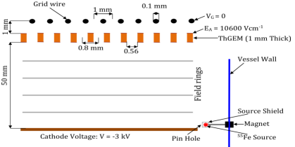
(a) Detector configuration.

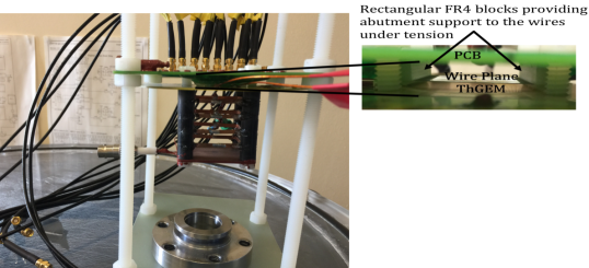
(b) Picture of the detector.

Figure 1: Illustration and picture of the hybrid detector. The black dots in 1(a) are the 100 $\mathrm{\SIUnitSymbolMicro m}$ stainless steel wires of the Multiwire-readout while orange rectangles mark the boundaries of the ThGEM holes. Light grey lines in 1(a) are the field rings and the red star is ⁵⁵Fe or ²⁴¹Am source. The E${}_{\text{A}}$ and V${}_{\text{G}}$ labels are the avalanche electric field and grid voltage, respectively. In 1(b) is a photograph of the detector when placed on the transparent lid of the vacuum vessel, showing the copper-plate cathode, field cage, ThGEM, wire-plane and SMC cables for connecting the wires to amplifiers (colour online).

The diameter and pitch of the hexagonally arranged circular ThGEM holes was 0.56 $\mathrm{mm}$ and 0.8 $\mathrm{mm}$, respectively. A cross section of the ThGEM is shown in Figure 1(a). Either side of the ThGEM holes were enclosed by an additional 0.04 $\mathrm{mm}$ rim, etched on the copper-clads to prevent electrostatic hole-edge discharges and ensure that electric field lines are centred on the ThGEM holes for optimal ion collection and field ionization for the avalanche process. The rim size can affect the performance of a ThGEM based detector. For instance, increasing the rim size of the ThGEM from 0.04 $\mathrm{mm}$ to 0.09 $\mathrm{mm}$ in a Garfield simulation [36], resulted in 86$\mathrm{\char 37\relax}$ loss of initial electrons into the copper cladding and dielectric FR4 material. It is important to point out that this is one of the early set of ThGEMs produced by CERN, so it does not represent an optimal design. The one-plane Multiwire readout was made using 100 $\mathrm{\SIUnitSymbolMicro m}$ diameter stainless steel wires, placed on a custom made printed circuit board at 1 $\mathrm{mm}$ pitch. The wire plane was then mounted on the induction side of the ThGEM at a ThGEM-Multiwire separation of 1 $\mathrm{mm}$. The sensitivity of such hybrid detector configuration can be improved in future designs by ensuring that the wire pitch is equal to the ThGEM hole pitch.

A field cage was designed and constructed to maintain a uniform drift field [37, 38] within the 2 $\mathrm{cm}$ $\times$ 2 $\mathrm{cm}$ $\times$ 5 $\mathrm{cm}$ detector volume as shown in Figure 1(b). This was achieved by stepping down the high-voltage applied to the copper-plate cathode through a series of five, 33 $\mathrm{M\SIUnitSymbolOhm}$ resistors connected to four series of copper field rings. To complete the circuit, the last field cage ring was connected to ground through the fifth successive resistor. The detector was then built by mounting the ThGEM-Multiwire readout on the field-cage with the ThGEM (charge transfer) side of the readout facing the drift volume as shown in Figure 1.

The full data flow path from the read-out wire to storage disk is shown in Figure 2.

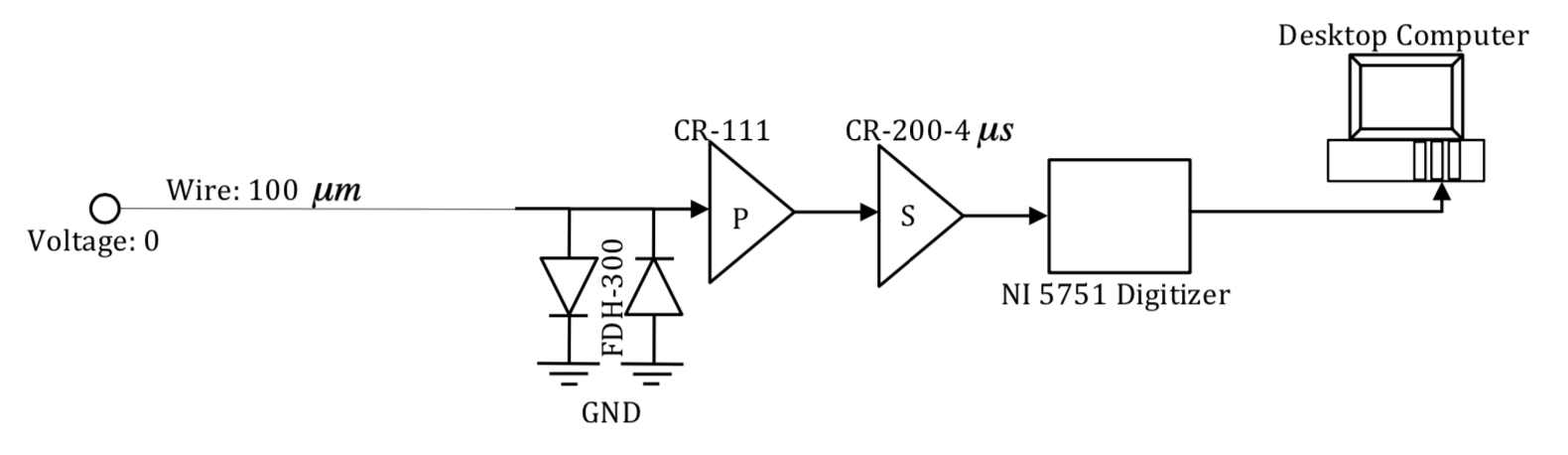
Figure 2: Path of the data flow. Arrows show the direction of the data flow.

During an operation, the charge transfer side of the ThGEM was biased to ensure that the drift field is maintained before the drifting anions are field-ionized for electron avalanche. The avalanche process and signal multiplication was induced by setting the opposite (induction) side of the ThGEM to a sufficient and more positive potential. By biasing the wire potential to 0 $\mathrm{V}$, avalanche electrons induce equivalent current [37, 38, 39, 40] on the wires as they follow the charge trajectories to the induction side of the ThGEM as shown in Figure 3.

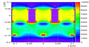
(a) Electric field contour.

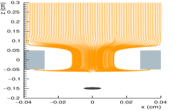
(b) Charge trajectory.

Figure 3: Electric field contour around three ThGEM holes and wires is shown in 3(a) while the charge trajectory through a ThGEM hole and around a read-out wire is shown in 3(b) as obtained with a Garfield simulation by biasing the drift field, charge transfer and induction sides of the ThGEM and read-out wires to $-700$ $\mathrm{V}\text{\,}{\mathrm{cm}}^{-1}$, $-450$ $\mathrm{V}$, $+600$ $\mathrm{V}$, and 0 $\mathrm{V}$, respectively. The colour scale in 3(a) shows the strength of the electric field measured in $\mathrm{V}\text{\,}{\mathrm{cm}}^{-1}$.

For a simple case where an electrode is set to voltage $V$ while other surrounding electrodes are grounded, the current $i_{t}$ induced by a charge $e$ moving along a trajectory $x_{t}$ towards the electrode can be defined as [37]:

$$i_{t}=-\frac{e}{V}E_{n}[x_{t}]v_{t}\,,$$ (1)

where $E_{n}$ is electric field of the electrode when the charge $e$ is removed while $v_{t}$ is the instantaneous velocity of the charge. The induced charge $Q$ over a given time $t$ can then be determined using:

$$Q=\int_{0}^{t}i_{t}dt\,.$$ (2)

Induced charge signals were used as avalanche electrons can reattach to SF${}_{\text{6}}$ to form anions while drifting from the induction side of the ThGEM to the charge collection wires. To do this, gas gain obtained from charge signals collected on the induction side of the ThGEM were measured and compared to the effective gain from induced charge signals on the wires. This was found to be consistent at similar detector conditions.

Garfield simulations were used to determine the operational voltage configurations for the detector. For instance, typical operational drift field range of $-300~{}$\mathrm{V}\text{\,}{\mathrm{cm}}^{-1}$~{}\text{to}~{}-700$ $\mathrm{V}\text{\,}{\mathrm{cm}}^{-1}$, charge transfer ThGEM voltage of $-450$ $\mathrm{V}$ and induction ThGEM voltage of $+600$ $\mathrm{V}$ and wire bias voltage of 0 $\mathrm{V}$ were used. An electric field contour and the expected charge trajectory in this voltage configuration are shown in Figure 3. The high electric field gradient around the vicinity of the charge transfer side of the ThGEM (see Figure 3(a)) induces the field ionization process. Positive (inverted) charge signals were induced on the surrounding wires by electromagnetic distortions caused by the motion of avalanche electrons towards the wires as they proceed to the induction side of the ThGEM. These induced currents on the wires were successively amplified using Cremat CR-111 pre-amplifiers and CR-200-4$\mathrm{\SIUnitSymbolMicro s}$ gaussian shaping amplifiers. As shown in Figure 2, a pair of grounded inverse parallel FDH-300 diodes were added between the pre-amplifiers and the wires to protect the amplifiers from power surge. Amplified signals were digitised using an NI 5751 digitizer controlled through a NI PXI-7953R FlexRIO FPGA and saved to disk for analyses. Due to the capacity of the digitizer, only 16 wire channels were instrumented. An FPGA [41] and LabVIEW [42] based data acquisition system (DAQ) was developed for online data quality monitoring and run control. A picture of the experimental setup stand is shown in Figure 4.

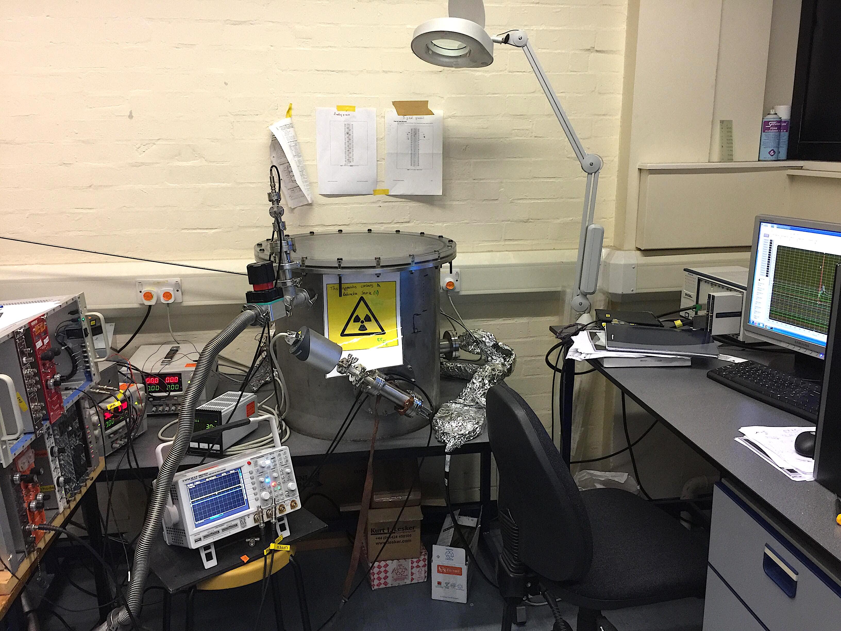
Figure 4: Picture of the experimental setup stand showing high voltage power supplies in NIM crates used to bias the copper-plate cathode, ThGEM and wires. The d.c. power supplies that power the amplifiers are also shown with the vacuum vessel, pressure gauge/monitor, NI digitizer and the data computer.

The white dual channeled ISEG NHQ 238L NIM cassette high voltage power supply shown in Figure 4 powered the copper-plate cathode and the charge transfer side of the ThGEM while the red dual channeled Bertan 377P power supply biased the induction side of the ThGEM and the read-out wires. The BST PSM 2/2A d.c. power supplies shown in Figure 4 were used to bias the Cremat amplifiers which are located inside the vacuum vessel to minimise noise distortions. A Leybold Ceravac CTR-101 pressure gauge was used to monitor the pressure of the 96 $\mathrm{l}$ vacuum vessel.

3 Detector Calibration

Gain measurement was performed to investigate the detector performance using X-rays from the electron capture decay of ${}^{\text{55}}$Fe source to ${}^{\text{55}}$Mn. As shown in Figure 1(a) the source was positioned close to the copper-plate cathode to irradiate the detector fiducial volume. To achieve this, the source was bonded to the tip of a 5 $\mathrm{cm}$ M6 nylon studding glued to a Neodymium disc magnet and attached to the inside wall of the vessel. This was magnetically coupled to a second magnet on the outside vessel wall which was used to control the source position in the vessel. Ionization electrons from X-ray interactions with the target gas through photoelectric effect - attach to the electronegative SF${}_{\text{6}}$ to form anions. As described in Sections 1 and 2, these anions drift in a uniform field to the ThGEM for field ionization and electron avalanche. Signal pulses induced on the wires from this process were amplified and recorded to disk at a frequency of 1 $\mathrm{MHz}$ per channel, without any hardware trigger as the pulses were small (for instance, $>$5 $\mathrm{mV}$ in 30 $\mathrm{Torr}$ of SF${}_{\text{6}}$). All signal pulses on each of the 16 wires with amplitude $>$5 $\mathrm{mV}$ threshold were analysed in the ${}^{\text{55}}$Fe runs to reject pedestal and electronic noise. Pulses with $>$3 $\mathrm{V}$ amplitude were not included in the analysis to remove sparks and events that saturate the amplifiers and the digitizer.

Background events due to radioactive decays from detector materials (at relevant energy) which could mimic the $<$2 wire channels trigger from the ${}^{\text{55}}$Fe X-ray interactions are expected to be minimal in the short exposure time (about 2 $\mathrm{h}$) of this source run. To determine the pulse area, any charge that passed the analysis threshold on each of the signal channels were integrated from the 10 $\mathrm{\SIUnitSymbolMicro s}$ time before the pulse rising edge crosses the threshold to the 10 $\mathrm{\SIUnitSymbolMicro s}$ time after the pulse falling edge crosses the threshold. The energy spectrum of events that passed the analysis cuts is shown in Figure 5.

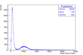
(a) Data spectrum from the Fe55 run.

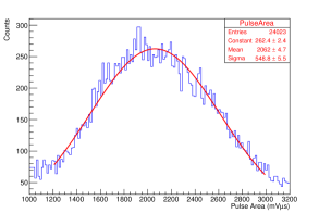
(b) Zoomed-in version of the Fe55 peak.

Figure 5: Energy spectrum of 5.9 $\mathrm{keV}$ X-rays from ${}^{\text{55}}$Fe source. All the events that passed the analyses cuts are shown in 5(a). This includes electronic noise and the X-ray events from the ${}^{\text{55}}$Fe source while 5(b) zooms-in on peak of the X-ray events. Red line is a gaussian fit to the X-ray events (colour online).

The peak of a gaussian fit on the observed spectrum of the X-ray data is 2062 $\pm$ 5 $\mathrm{mV}\text{\,}\mathrm{\SIUnitSymbolMicro s}$. To understand the detector gas gain, the amplifier gain was calibrated using test pulses of 14 $\mathrm{mV}$ (minimum output voltage of the pulser) and 20 $\mathrm{mV}$ to 90 $\mathrm{mV}$ amplitude at 10 $\mathrm{mV}$ interval. To do this, each of the test pulse signals was connected to the test input of the pre-amplifiers. The $\mathrm{mV}$-scale test pulses were converted to charge signals through a 1 $\mathrm{pF}$ test capacitor of the pre-amplifiers. The charge output of the pre-amplifier was then coupled to the shaping amplifier for further amplification and shaping. The shaped pulse signals were then digitized, saved to disk and analysed using the same analyses algorithm used in the X-ray data shown in Figure 5. As in the X-ray data, a gaussian was fitted on each of the amplifier calibration data and the peak of the fits were extracted and analysed as a function of the expected detector gas gain from 5.9 $\mathrm{keV}$ X-rays from ${}^{\text{55}}$Fe exposures. Results from the calibration pulse analyses are shown as a function of the expected detector gas gain in Figure 6.

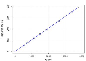
Figure 6: Integral charge from amplifier calibration pulses shown as a function of expected gas gain from ${}^{\text{55}}$Fe X-ray interactions. The blue solid line is a linear fit on the data (colour online).

The expected gas gain shown in Figure 6 was determined by converting each of the observed test charge to their equivalent number of ion pairs (NIPs) using:

$$NIPs_{o}=\frac{CV}{e}\,,$$ (3)

where $NIPs_{o}$ is the observed number of ion pairs, $C$ is the test capacitance of the amplifier, $V$ is the test pulse in $\mathrm{mV}$ and $e$ is the electronic charge. The expected number of ion pairs ($NIPs_{e}$) from an ${}^{\text{55}}$Fe X-ray was determined using:

$$NIPs_{e}=\frac{E}{W}\,,$$ (4)

where $E$ is the 5.9 $\mathrm{keV}$ energy of ${}^{\text{55}}$Fe X-rays while $W$ is the mean energy required to create an electron-ion pair in SF${}_{\text{6}}$ target gas - measured to be 35.45 $\mathrm{eV}$ in Ref. [43]. This implies that the ${}^{\text{55}}$Fe X-ray will produce 166.4 electron-ion pairs after an interaction with the target gas before the electron avalanche. Hence, the detector gas gain is defined as the ratio of the $NIPs_{o}$ to the $NIPs_{e}$. Using parameters of the linear fit ($\text{Q}_{\text{A}}=2G+6$) in Figure 6, where G and $\text{Q}_{\text{A}}$ are the effective gas gain and the integral charge, respectively. These parameters and the observed integral charge from the ${}^{\text{55}}$Fe analyses yield a gain of 1028 $\pm$ 3.

Table 1: Detector parameters used in the detector calibration run performed in 30 $\mathrm{Torr}$ of pure SF${}_{\text{6}}$ target gas. The V, E, $\Delta\text{V}_{\text{A}}$ and $\text{E}_{\text{A}}$ parameters are cathode voltage, drift field, avalanche voltage and avalanche fields, respectively. The E/N ($\text{E}_{\text{A}}/\text{N}$) is the reduced drift (avalanche) field while N is the gas density computed to be $9.7\times 10^{17}$ ${\mathrm{cm}}^{-3}$.

V ($\mathrm{V}$) E ($\mathrm{kV}\text{\,}{\mathrm{cm}}^{-1}$) E/N ($10^{-17}$ $\mathrm{V}\text{\,}{\mathrm{cm}}^{2}$) $\Delta\text{V}_{\text{A}}$ ($\mathrm{V}$) $\text{E}_{\text{A}}$ ($\mathrm{kV}\text{\,}{\mathrm{cm}}^{-1}$) $\text{E}_{\text{A}}\text{/N}$ ($10^{-17}$ $\mathrm{V}\text{\,}{\mathrm{cm}}^{2}$) 3000 0.6 62 1055 10.6 1092

For details of drift and avalanche fields used in this detector calibration run, see Table 1. This is using a drift (avalanche) field of 600 $\mathrm{V}\text{\,}{\mathrm{cm}}^{-1}$ (10.6 $\mathrm{kV}\text{\,}{\mathrm{cm}}^{-1}$) in 30 $\mathrm{Torr}$ of pure SF${}_{\text{6}}$ gas - equivalent to E/N and $\text{E}_{A}/\text{N}$ of 62 $\times~{}10^{-17}$ $\mathrm{V}\text{\,}{\mathrm{cm}}^{2}$ and 1092 $\times~{}10^{-17}$ $\mathrm{V}\text{\,}{\mathrm{cm}}^{2}$, respectively. Here, E/N is the reduced drift field, $\text{E}_{\text{A}}/\text{N}$ is the reduced avalanche field and N is the gas density computed to be $9.7\times 10^{17}$ ${\mathrm{cm}}^{-3}$, for more on the N parameter, see section 4.2. Hence, the calibration gain result does not represent the highest achievable gain of the detector as higher reduced avalanche fields with sufficient reduced drift field configurations can yield higher effective gas gains. The investigation of the highest achievable effective gain of the detector is beyond the scope this paper.

4 Ionization Tracking Capabilities

To further understand the detector performance and demonstrate the ionization tracking capabilities of the detector, the ${}^{\text{55}}$Fe source discussed in Section 3 was replaced with an ${}^{\text{241}}$Am source which emits 5.5 $\mathrm{MeV}$ alphas as it decays to ${}^{\text{237}}$Np. This is such that the mean free path of alphas from the source was few $\mathrm{mm}$ away from the cathode. As discussed in Sections 2 and 3, ionization electrons along the interaction track of the ionizing alpha, as it traverses the detector fiducial volume attach to the electronegative SF${}_{\text{6}}$ to form anions. These anions were drifted in the uniform electric field to the high field region of the detector readout for field ionization and subsequent electron avalanche. Signal pulses induced on the wires by this process were pre-amplified, shaped, digitized and saved to disk for analyses.

4.1 Events Pre-Selection Analysis and Data Quality

Seven alpha source runs were performed at different reduced drift fields to validate the dependency of the field ionization process on the gradient of the ThGEM charge transfer field relative to the drift field. This is using a constant reduced avalanche field of 1449 $\pm$ 1 $\times~{}10^{-17}$ $\mathrm{V}\text{\,}{\mathrm{cm}}^{2}$ as shown in Table 2, except in the seventh $\text{E}_{\text{A}}/\text{N}$ field run where it was increased by $\sim$1% to 1461 $\pm$ 1 $\times~{}10^{-17}$ $\mathrm{V}\text{\,}{\mathrm{cm}}^{2}$ to investigate the detector response to a higher $\text{E}_{\text{A}}/\text{N}$ field. The expectation is that this small increase in the reduced avalanche field should increase the effective gain of the detector.

Table 2: Detector parameters used in the ionization tracking studies performed in 20 $\mathrm{Torr}$ of pure SF${}_{\text{6}}$ target gas. The V, E, $\Delta\text{V}_{\text{A}}$ and $\text{E}_{\text{A}}$ parameters are cathode voltage, drift field, avalanche voltage and avalanche fields, respectively. The E/N ($\text{E}_{\text{A}}/\text{N}$) is the reduced drift (avalanche) field while N is the gas density computed to be $6.5\times 10^{17}$ ${\mathrm{cm}}^{-3}$.

V ($\mathrm{V}$) E ($\mathrm{kV}\text{\,}{\mathrm{cm}}^{-1}$) E/N ($10^{-17}$ $\mathrm{V}\text{\,}{\mathrm{cm}}^{2}$) $\Delta\text{V}_{\text{A}}$ ($\mathrm{V}$) $\text{E}_{\text{A}}$ ($\mathrm{kV}\text{\,}{\mathrm{cm}}^{-1}$) $\text{E}_{\text{A}}\text{/N}$ ($10^{-17}$ $\mathrm{V}\text{\,}{\mathrm{cm}}^{2}$) 1800 0.36 56 933 9.33 1449 2000 0.40 62 933 9.33 1449 2200 0.44 68 933 9.33 1449 2400 0.48 75 933 9.33 1449 2600 0.52 81 933 9.33 1449 2800 0.56 87 933 9.33 1449 3000 0.60 93 941 9.41 1461

An example of a raw alpha track oriented towards the cathode as seen on the LabVIEW based DAQ is shown in Figure 7.

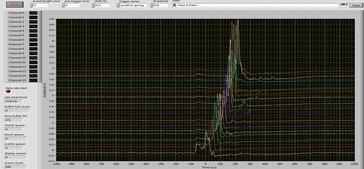
Figure 7: An example from part of 5.5 $\mathrm{MeV}$ alpha track observed in the hybrid detector with 30 $\mathrm{Torr}$ of pure SF${}_{\text{6}}$ target gas. The full alpha track is expected to be 27.9 $\mathrm{cm}$ long on average, as determined from SRIM [44] simulations. Channel 0 is closer to the ${}^{\text{241}}$Am source.

The alpha track is preceded by a low-energy track, likely from radioactive decays in the detector materials within the opposite vicinity of the source location. For this alpha track, the source was placed few $\mathrm{mm}$ away from the ThGEM to observe a clear charge arrival time delay from tracks oriented towards the cathode. It can be seen that the low-energy track is oriented along the expected mean free path of the source-alphas hence, the resulting ionization charge arrived the readout at about same time. The clear observation of delays between induced charge signals on adjacent wires of the alpha track due to the expected slow negative ion drift properties is of more importance to the work reported here. The wire shown as Channel 0 on the DAQ is closer to the alpha source. The 210 $\mathrm{\SIUnitSymbolMicro s}$ delay between channels 0 and  15 of the alpha track signal shown in Figure 7 is due to the drift times of the anions which depends on the incident angle (within the source subtended solid angle) of the alpha track. The observed wiggle on each of the DAQ channel after the main alpha signal pulse is due to amplifier responses and so were not included in the analysis.

Events with $>$40 $\mathrm{mV}$ pulse amplitude threshold were analysed further. This is to remove pedestal and electronics noise from the analysis. As discussed in Section 3, events with $>$3 $\mathrm{V}$ pulse amplitude were also removed. Sparks and other noise pulses with short rise-times were rejected by selecting only events with $>$9 $\mathrm{\SIUnitSymbolMicro s}$ rise-time and full-width at half maximum (FWHM) of 8 $\mathrm{\SIUnitSymbolMicro s}$ to 60 $\mathrm{\SIUnitSymbolMicro s}$. An example of the pulse amplitude and FWHM obtained from a 56 $\times~{}10^{-17}$ $\mathrm{V}\text{\,}{\mathrm{cm}}^{2}$ reduced drift field run (see Table 2 for more details) in 20 $\mathrm{Torr}$ of pure SF${}_{\text{6}}$ gas are shown in Figure 8.

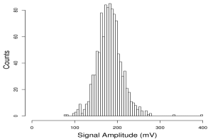
(a) Pulse amplitude.

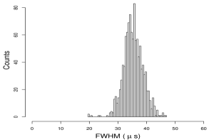
(b) Full width at half maximum.

Figure 8: Distribution of pulse amplitude and full width at half maximum observed from alpha tracks at a reduced drift field of 56 $\times~{}10^{-17}$ $\mathrm{V}\text{\,}{\mathrm{cm}}^{2}$ and avalanche field of 9.33 $\mathrm{kV}\text{\,}{\mathrm{cm}}^{-1}$ in 20 $\mathrm{Torr}$ of pure SF${}_{\text{6}}$ target gas.

The average pulse amplitude (FWHM) observed from this run is 181 $\pm$ 2 $\mathrm{mV}$ (36 $\pm$ 0.2 $\mathrm{\SIUnitSymbolMicro s}$). This long FWHM and slow rise-time is consistent with expectations from negative ion drift in the electronegative SF${}_{\text{6}}$ target gas.

As discussed in Section 3, the effective detector gas gain in each of these runs was measured using alpha events as in Ref. [32]. To do this, a cumulative integral charge in a fixed time window, around the trigger time for a given signal channel was computed. The maximum from this computation was recorded as the channel charge integral. The sum of this charge integral over all the 16 signal channels is the total integral charge for a given alpha track. This method helps to remove the effect of the pedestal noise from the integral charge computations. Samples of total integral charge distributions as observed from two of these ionization tracking runs are shown in Figure 9.

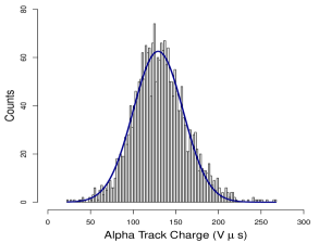
(a) Charge at 68 $\times~{}10^{-17}$ $\mathrm{V}\text{\,}{\mathrm{cm}}^{2}$ E/N mode.

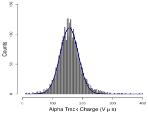
(b) Charge at 87 $\times~{}10^{-17}$ $\mathrm{V}\text{\,}{\mathrm{cm}}^{2}$ E/N mode.

Figure 9: Distribution of total integral charge from alpha tracks as observed from reduced drift field runs of 68 $\times~{}10^{-17}$ $\mathrm{V}\text{\,}{\mathrm{cm}}^{2}$ and 87 $\times~{}10^{-17}$ $\mathrm{V}\text{\,}{\mathrm{cm}}^{2}$, respectively. These data were recorded at an avalanche field of 9.33 $\mathrm{kV}\text{\,}{\mathrm{cm}}^{-1}$ in 20 $\mathrm{Torr}$ of pure SF${}_{\text{6}}$ target gas. Dark blue lines are gaussian fits on the data (colour online).

There are no visible pedestal noise in Figure 9 as seen in Figure 5(a) due to the lower exposure-times in the alpha runs because the source activity is 2 orders of magnitude higher than that of the X-ray runs in Section 3. Also, as described above, the charge threshold and cuts applied in the alpha analyses are more stringent for the pedestal noise than in the X-ray data analyses. As described in Section 3, the peak of the gaussian fits in Figures 9(a) and 9(b) were extracted and used as the effective track integral charge for the effective gain computations. The mean integral charge extracted from the fits in Figure 9, are 133 $\pm$ 1 $\mathrm{V}\text{\,}\mathrm{\SIUnitSymbolMicro s}$ and 158 $\pm$ 2 $\mathrm{V}\text{\,}\mathrm{\SIUnitSymbolMicro s}$ for reduced drift field runs of 68 $\times~{}10^{-17}$ $\mathrm{V}\text{\,}{\mathrm{cm}}^{2}$ and 87 $\times~{}10^{-17}$ $\mathrm{V}\text{\,}{\mathrm{cm}}^{2}$, respectively. Similar analyses were performed on the remaining 5 alpha runs taking at different reduced drift fields.

To convert these results to an effective gain measurement, a SRIM simulation was performed to determine the fraction of the 5.5 $\mathrm{MeV}$ alpha energy that was deposited within the detector fiducial volume as the tracks are expected to be longer than the detector width. This was found to be 0.22 $\mathrm{MeV}$ in average, which translates to 4% of the total alpha energy. Using this average alpha deposited energy and calibration results from analyses of the pulse calibration runs described in Section 3, the effective gas gain in each of the alpha runs was determined. The effective gain results from these measurements are shown as a function of the reduced drift fields in Figure 10.

Figure 10: Effective gas gains in 20 $\mathrm{Torr}$ of pure SF${}_{\text{6}}$ gas shown as a function of reduced drift field. Reduced avalanche fields used in the left and right regions (before and after) of the dashed blue line is 1449  $\times~{}10^{-17}$ $\mathrm{V}\text{\,}{\mathrm{cm}}^{2}$ and 1461 $\times~{}10^{-17}$ $\mathrm{V}\text{\,}{\mathrm{cm}}^{2}$, respectively. Results are from ²⁴¹Am alpha tracks.

The effective gas gain results shown in Figure 10 increase with the reduced drift field as expected (at low reduced drift fields). This is due to a more positive field gradient in the charge transfer region of the ThGEM as the reduced drift field increases - resulting in better negative ion transparency. The observed effective gas gain in Figure 10 plateaued from the 75 $\times~{}10^{-17}$ $\mathrm{V}\text{\,}{\mathrm{cm}}^{2}$ to 87 $\times~{}10^{-17}$ $\mathrm{V}\text{\,}{\mathrm{cm}}^{2}$ reduced drift field runs. This is consistent with expectations from reaching the optimal negative ion-drift transparency for the constant reduced avalanche field. The observed rise in the effective gas gain for the reduced drift field run of 93 $\times~{}10^{-17}$ $\mathrm{V}\text{\,}{\mathrm{cm}}^{2}$ (at optimal ion-drift transparency) is due to the higher avalanche field in this run as shown in Table 2. However, the drift velocity and mobility of anions are independent of the effective gas gain so these observed plateau and rise in the detector gain should not affect our measurements. These results indicate that a gas gain of 2.5 $\times~{}10^{3}$ is feasible with the ThGEM-multiwire hybrid setup in SF${}_{\text{6}}$ target gas.

4.2 Drift Velocity and Mobility Measurements for SF${}_{\text{6}}$ Anions

To extract the drift velocity and mobility of SF${}_{\text{6}}$ anions, only alpha tracks that made angles of $>81\begin{subarray}{c}+1\\ -0.5\end{subarray}$$\mathrm{\SIUnitSymbolDegree}$ with the cathode were selected from each of the runs described in Section 4. For details of drift and avalanche field configurations for each of the runs, see Table 2. As shown in Figure 11, these tracks were expected to induce signals only on the first 8 wires of the detector.

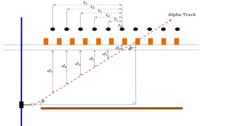
Figure 11: Illustration of alpha track selection cuts and parametizations used in the SF${}_{\text{6}}$ anion drift velocity and mobility measurements. Angles $\theta$ and $\phi$ are $81\begin{subarray}{c}+1\\ -0.5\end{subarray}$$\mathrm{\SIUnitSymbolDegree}$ and $9\begin{subarray}{c}+0.5\\ -1\end{subarray}$$\mathrm{\SIUnitSymbolDegree}$, respectively.

Hence, events that recorded hits on these 8 wires, only were selected for further analysis. A hit here is charge induced on a wire that produced a pulse amplitude that passed the analyses threshold. Between 0.2% to 2.3% of the total events on disk in the ionization tracking runs passed these cuts and were used in the ion drift velocity and mobility measurements.

It can be seen in Figure 11 that there is no drift distance for the most probable ionization charge that could end on the 7${}^{\text{th}}$ and 8${}^{\text{th}}$ wires due to the proximity of the interaction vertex to the field ionization region of the ThGEM and readout wire plane, respectively. Hence, signals on these two wires were not included in the drift velocity and mobility computation. The charge arrival time information from the 6${}^{\text{th}}$ wire served as the reference for charge drift times recorded on the first 5 wires.

The vertical drift distances (d${}_{\text{1}}$, d${}_{\text{2}}$, d${}_{\text{3}}$, d${}_{\text{4}}$ and d${}_{\text{5}}$) between the expected start positions of charge clusters arriving on the first 5 wires and the start position of charge cluster arriving on the 6${}^{\text{th}}$ wire (after traveling a d${}_{\text{0}}$ distance) was determined using $\text{x}_{\text{i}}\tan\theta$, see Figure 11 for more details. Here, $\text{x}_{\text{i}}$ is the horizontal distance of the first 5 wires relative to the 6${}^{\text{th}}$ wire, so i is 1, 2, …, 5 while $\theta$ is the track mean free path-cathode angle determined to be $81\begin{subarray}{c}+1\\ -0.5\end{subarray}$$\mathrm{\SIUnitSymbolDegree}$. Charge drift times (t${}_{\text{1}}$, t${}_{\text{2}}$, t${}_{\text{3}}$, t${}_{\text{4}}$ and t${}_{\text{5}}$) for charge clusters arriving on these first 5 wires were computed as the temporal separation between their respective charge cluster arrival times and the arrival time, t${}_{\text{0}}$, of the charge cluster recorded on the reference 6${}^{\text{th}}$ wire. The gradient of a linear fit on a vertical drift distance vs drift time plot from a given run was recorded as the drift velocity, $v_{d}$, for that run.

The mobility, $\mu$, is defined in terms of $v_{d}$ as:

$$\mu=\frac{v_{d}}{E}\,,$$ (5)

where $E$ is the drift field. This can be converted to the reduced mobility $\mu_{0}$ by considering the operational gas density in each of the measurements for better comparison with other measurements using:

$$\mu_{0}=\frac{v_{d}}{E}\frac{N}{N_{0}}\,.$$ (6)

As mentioned in Section 3, $N$ is the gas density defined as $\frac{\rho A}{Mm}$ in ${\mathrm{cm}}^{-3}$, where $\rho$ is the gas density for the gas pressure used in a given measurement, $A$ is the Avagadro’s constant $6.0221\times 10^{23}$ ${\mathrm{mol}}^{-1}$ and $Mm$ is the molar mass of SF${}_{\text{6}}$ given as 146.06 $\mathrm{g}\text{\,}{\mathrm{mol}}^{-1}$. The $N_{0}$ (the Loschmidt constant) is the $N$ parameter computed at the standard temperature (0 $\mathrm{\SIUnitSymbolCelsius}$) and pressure (1 atm or 760 $\mathrm{Torr}$) which can be evaluated to obtain $2.6868\times 10^{19}$ ${\mathrm{cm}}^{-3}$. Results from the $v_{d}$ and $\mu_{0}$ measurements are shown in Table 3 and Figure 12 as a function of reduced drift fields for a given run in 20 $\mathrm{Torr}$ of SF${}_{\text{6}}$ target gas.

Table 3: Reduced drift field in each of the runs shown with the measured effective gas gain G, drift velocity $v_{d}$ and reduced mobility $\mu_{0}$. These measurements were performed in 20 $\mathrm{Torr}$ of pure SF${}_{\text{6}}$ target gas.

      E/N ($10^{-17}$$\mathrm{V}\text{\,}{\mathrm{cm}}^{2}$)       G       $v_{d}$ ($\mathrm{m}\text{\,}{\mathrm{s}}^{-1}$)       $\mu_{0}$ (${\mathrm{cm}}^{2}\text{\,}{\mathrm{V}}^{-1}\text{\,}{\mathrm{s}}^{-1}$)       56       1130 $\pm$ 90       80 $\pm$ 2       0.531 $\pm$ 0.013       62       1350  $\pm$ 100       89 $\pm$ 2       0.536 $\pm$ 0.012       68       1550 $\pm$ 100       99 $\pm$ 2       0.538 $\pm$ 0.011       75       1650 $\pm$ 100       108 $\pm$ 3       0.539 $\pm$ 0.015       81       1620 $\pm$ 90       117 $\pm$ 3       0.539 $\pm$ 0.016       87       1840  $\pm$ 110       129 $\pm$ 5       0.550 $\pm$ 0.020       93       2470 $\pm$ 160       138 $\pm$ 10       0.553 $\pm$ 0.041

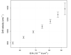
(a) Drift velocity.

(b) Reduced mobility.

Figure 12: Drift velocity and reduced mobility for SF${}_{\text{6}}$ anions shown as a function of reduced drift field. Only statistical uncertainties are quoted. See Table 2 and 3 for more details on detector parameters used in these measurements and results, respectively.

It can be seen in Figure 12(a) that the observed drift velocity increases with reduced drift field as expected. These observed $v_{d}$ results are consistent within errors with SF${}_{\text{6}}^{-}$ results in Ref. [24] for the relevant reduced drift field used in these measurements. The large uncertainties ($\pm$2 to $\pm$10 $\mathrm{m}\text{\,}{\mathrm{s}}^{-1}$) on these results are mainly due to systematics from relative wire-ThGEM hole positions and uncertainties in the estimation of the $\theta$ and $\phi$ angles for the selected alpha tracks. However, the observed reduced ion mobilities for the respective reduced drift field runs shown in Table 3 and Figure 12(b) are consistent within errors with SF${}_{\text{6}}^{-}$ results reported in Refs. [24, 45, 46, 47].

5 Conclusion

A ThGEM-Multiwire based hybrid time projection chamber (TPC) detector was designed, built and tested for the first time. Effective gas gain measured from the performance tests of the hybrid detector are in the range of $1130~{}\pm~{}90$ to $2470\pm 160$ at a reduced drift field E/N range of 56 $\times~{}10^{-17}$ $\mathrm{V}\text{\,}{\mathrm{cm}}^{2}$ to 93 $\times~{}10^{-17}$ $\mathrm{V}\text{\,}{\mathrm{cm}}^{2}$ in 20 $\mathrm{Torr}$ of pure SF${}_{\text{6}}$ target gas. Using the hybrid detector, the drift velocity and reduced ion mobility of SF${}_{\text{6}}$ anions were measured at this reduced drift field range. The observed drift velocity (reduced mobility) results were found to be between $80~{}\pm~{}2$ $\mathrm{m}\text{\,}{\mathrm{s}}^{-1}$ and $138~{}\pm~{}10$ $\mathrm{m}\text{\,}{\mathrm{s}}^{-1}$ ($0.53~{}\pm~{}0.01$ ${\mathrm{cm}}^{2}\text{\,}{\mathrm{V}}^{-1}\text{\,}{\mathrm{s}}^{-1}$ and $0.55~{}\pm~{}0.04$ ${\mathrm{cm}}^{2}\text{\,}{\mathrm{V}}^{-1}\text{\,}{\mathrm{s}}^{-1}$) in this reduced drift field range. The drift velocity and reduced ion mobility results from these measurements are consistent within errors with other published measurements in Refs. [24, 45, 46, 47].

Hence, the ThGEM-Multiwire technology has the potential to serve as a robust, low noise charge readout with known fine grain track resolution in the future massive directional dark matter detector known as CYGNUS-TPC.

References

References

- [1] G. Bertone, D. Hooper and J. Silk, Particle dark matter: Evidence, candidates and constraints, Phys. Reports 405 (5-6) (2005) 279-390.
- [2] M. Battaglieri et al., US Cosmic Visions: New Ideas in Dark Matter 2017: Community Report, arXiv: 1707.04591 (2017).
- [3] Particle Data Group, K. A. Olive et. al., Review of particle physics, Chin. Phys. C38 (9) (2014) 090001.
- [4] S. Ahlen et al., The Case for a Directional Dark Matter Detector and the Status of Current Experimental Efforts, Int. J. of Mod. Phys. A25 (01) (2010) 1-51.
- [5] F. Mayet et. al., A review of the discovery reach of directional Dark Matter detection, Physics Reports 627 (2016) 1-49.
- [6] D. N. Spergel Motion of the Earth and the detection of Weakly Interacting Massive Particles, Phys. Rev. D 37 (6) (1988) 1353-1355.
- [7] DRIFT Collaboration, J. B. R. Battat et al., First background-free limit from a directional dark matter experiment: results from a fully fiducialised DRIFT detector, Phys. Dark Univ. 9-10, (2015) 1-7.
- [8] P. Grothaus, M. Fairbairn and J. Monroe, Directional Dark Matter Detection Beyond the Neutrino Bound, Phys. Rev. D 90 (5) (2014) 055018.
- [9] C. A. J. O’Hare et al., Readout strategies for directional dark matter detection beyond the neutrino background, Phys. Rev. D 92 (6) (2015) 063518.
- [10] J. Billard, F. Mayet and D. Santos, Assessing the discovery potential of directional detection of dark matter, Phys. Rev. D 85 (3) (2012) 035006.
- [11] S. E. Vahsen et al., CYGNUS: Feasibility of a nuclear recoil observatory with directional sensitivity to dark matter and neutrinos, arXiv 2008.12587 (2020). https://arxiv.org/pdf/2008.12587.pdf.
- [12] J. B. R. Battat et al., Low threshold results and limits from the DRIFT directional dark matter detector, Astroparticle Physics 91 (2017) 65-74.
- [13] NEWAGE Collaboration, K. Nakamura et al., Direction-sensitive dark matter search with gaseous tracking detector NEWAGE-0.3b, Prog. Theor. Exp. Phys. 043F01 (2015) 261-266.
- [14] MIMAC Collaboration, D. Santos et al., MIMAC: MIcro-tpc MAtrix of Chambers for dark matter directional detection, J. Phys. Conf. Ser. 469, (2013) 012002.
- [15] D3 Collaboration, S. E. Vahsen et al., 3-D tracking in a miniature time projection chamber, Nucl. Instrum. Meth. A 788 (2015) 95-105.
- [16] DMTPC Collaboration, J. B. R. Battat et al., The Dark Matter Time Projection Chamber 4Shooter directional dark matter detector: Calibration in a surface laboratory, Nucl. Instrum. Meth. A 755, (2014) 6-19.
- [17] CYGNO Collaboration, G. Cavoto et al., Micro pattern gas detector optical readout for directional dark matter searches, Nucl. Instrum. Meth. A , 958, (2020) 162400.
- [18] D. P. Snowden-Ifft, C. J. Martoff and J. M. Burwell, Low pressure negative ion time projection chamber for dark matter search, Phys. Rev. D 61 (10) (2000) 101301.
- [19] J. B. R. Battat et al., First measurement of nuclear recoil head-tail sense in a fiducialised WIMP dark matter detector, Journal of Instrumentation 11 (10) (2016) P10019.
- [20] J. B. R. Battat et al., Measurement of directional range components of nuclear recoil tracks in a fiducialised dark matter detector, Journal of Instrumentation 12 (10) (2017) P10009.
- [21] N. L. Aleksandrov, Three-body electron attachment to a molecule, Soviet Physics Uspekhi 31 (2) (1988) 101-118.
- [22] E. P. Grimsrud, S. Chowdhury, and P. Kebarle, Electron affinity of SF6 and perfluoromethylcyclohexane. The unusual kinetics of electron transfer reactions , where A=SF6 or perfluorinated cyclo-alkanes, J. Chem. Phys 83 (1985) 1059.
- [23] A. C. Ezeribe et al., Demonstration of radon removal from SF6 using molecular sieves, Journal of Instrumentation 12 (09), (2017) P09025.
- [24] N. S. Phan et al., The novel properties of SF6 for directional dark matter experiments, Journal of Instrumentation 12 (02) (2017) P02012.
- [25] D. P. Snowden-Ifft, Discovery of multiple, ionization-created CS2 anions and a new mode of operation for drift chambers, Review of Scientific Instruments 85 (2014) 013303.
- [26] D. R. Tovey et al., A New model independent method for extracting spin dependent (cross-section) limits from dark matter searches, Phys. Lett. B 488, (2000) 17-26.
- [27] V. A. Bednyakov, Aspects of Spin-Dependent Dark Matter Search, Physics of Atomic Nuclei 67 (11), (2004) 1931-1941.
- [28] G. Charpak and F. Sauli, Multiwire proportional chambers and drift chambers, Nuclear Instruments and Methods 162 (1), (1979) 405-428.
- [29] T. Ferbel, Experimental Techniques in High-Energy Nuclear and Particle Physics, , World Scientific, (1991) 78-188.
- [30] G. J. Alner et al., The DRIFT-II dark matter detector: Design and commissioning, Nucl. Instrum. Meth. A 555 (1), (2005) 173-183.
- [31] F. Sauli, The gas electron multiplier (GEM): Operating principles and applications, Nucl. Instrum. Meth. A 805, (2016) 2-24.
- [32] J. Burns et al., Characterisation of large area THGEMs and experimental measurement of the Townsend coefficients for CF4, Journal of Instrumentation 12 (10), (2017) T10006.
- [33] H. Ishiura et al., MPGD simulation in negative-ion gas for direction-sensitive dark matter searches, in: 6th International Conference on Micro Pattern Gaseous Detectors (MPGD2019) La Rochelle, France, May 5-10, 2019. https://iopscience.iop.org/article/10.1088/1742-6596/1498/1/012018/pdf.
- [34] A. C. Ezeribe et al., Performance of 20:1 multiplexer for large area charge readouts in directional dark matter TPC detectors, Journal of Instrumentation 13 (02), (2018) P02031.
- [35] A. C. Ezeribe, Towards a massive directional dark matter detector: CYGNUS-TPC, Ph.D. thesis, University of Sheffield, Sheffield, United Kingdom (2016).
- [36] R. Veenhof and H. Schindler, Garfield++ - simulation of tracking detectors, http://garfieldpp.web.cern.ch/garfieldpp (1984-2018).
- [37] W. Blum, W. Riegler, and L. Rolandi, Eds: Chao A. , Fabjan C. W., and Zimmermann F., Particle Detection with Drift Chambers, 2 edition, Springer Verlag,(2008).
- [38] G. F. Knoll, Radiation detection and measurement, 3 edition, John Wiley & Sons Inc., (2010).
- [39] W. Shockley, Currents to Conductors Induced by a Moving Point Charge, Journal of Applied Physics 9 (1938) 635-636.
- [40] S. Ramo, Currents induced by electron motion, Proc. Ire. 27 (1939) 584-585.
- [41] U. Farooq, Z. Marrakchi and H. Mehrez, FPGA Architectures: An Overview. In: Tree-based Heterogeneous FPGA Architectures, Springer, New York, NY (2012).
- [42] C. Elliott et al., National Instruments LabVIEW: A Programming Environment for Laboratory Automation and Measurement, Journal of the Association for Laboratory Automation 12 (1) (2007) 17-24.
- [43] Y. H. Hilal and L. G. Christophorou, The energy to produce an electron-ion pair in SF and SF/N gas mixtures, Journal of Physics D: Applied Physics 20 (7) (1987) 975-976.
- [44] J. F. Ziegler, M. D. Ziegler and J. P. Biersack, SRIM -The stopping and range of ions in matter, Nuclear Instruments and Methods in Physics Research Section B: Beam Interactions with Materials and Atoms 268 (11) (2010) 1818-1823.
- [45] I. A. Fleming and J. A. Rees, The drift velocities of ions in sulphur hexafluoride, Journal of Physics B: Atomic and Molecular Physics 2 (7) (1969) 777-779.
- [46] P. L. Patterson, Mobilities of Negative Ions in SF6, The Journal of Chemical Physics 53 (2) (1970) 696-704.
- [47] J. de Urquijo et al., Mobility and longitudinal diffusion of SF5-and SF6-in SF6, Journal of Physics D: Applied Physics 24 (5) (1991) 664-667.