Automated design of error-resilient and hardware-efficient deep neural networks

Abstract

Applying deep neural networks (DNNs) in mobile and safety-critical systems, such as autonomous vehicles, demands a reliable and efficient execution on hardware. Optimized dedicated hardware accelerators are being developed to achieve this. However, the design of efficient and reliable hardware has become increasingly difficult, due to the increased complexity of modern integrated circuit technology and its sensitivity against hardware faults, such as random bit-flips. It is thus desirable to exploit optimization potential for error resilience and efficiency also at the algorithmic side, e.g. by optimizing the architecture of the DNN. Since there are numerous design choices for the architecture of DNNs, with partially opposing effects on the preferred characteristics (such as small error rates at low latency), multi-objective optimization strategies are necessary. In this paper, we develop an evolutionary optimization technique for the automated design of hardware-optimized DNN architectures. For this purpose, we derive a set of easily computable objective functions, which enable the fast evaluation of DNN architectures with respect to their hardware efficiency and error resilience solely based on the network topology. We observe a strong correlation between predicted error resilience and actual measurements obtained from fault injection simulations. Furthermore, we analyze two different quantization schemes for efficient DNN computation and find significant differences regarding their effect on error resilience.

1 Introduction

The application of DNN in safety-critical perception systems, for example AV, poses some challenges on the design of the underlying hardware platforms. On the one hand, efficient and fast accelerators are needed, since DNN for computer vision exhibit massive computational requirements Lin et al. (2018). On the other hand, resilience against random hardware faults has to be ensured. In many driving scenarios, entering a fail-safe state is not sufficient, but fail-operational behavior and fault tolerance are required Koopman and Wagner (2016). However, fault tolerance techniques at the hardware level often entail large redundancy overheads in silicon area, latency, and power consumption. These overheads stand in contrast to the low-power and low-latency requirements of embedded real-time DNN accelerators. Reliability concerns in nanoscale integrated circuits, for instance soft errors in memory and logic, represent an additional challenge for the realization of fault tolerance mechanisms at the hardware level Aitken et al. (2015); Gomez et al. (2014); Henkel et al. (2013); Mutlu (2017); Sridharan et al. (2015). Moreover, techniques such as near-threshold computing Dreslinski et al. (2010) and approximate computing Mittal (2016) are desirable to meet power constraints, but can further increase error rates.

To overcome these challenges, one option is to exploit error resilience at the algorithm level and allow for a certain degree of inaccuracy at the hardware level. This is referred to as cross-layer resilience Carter et al. (2010). Due to the implicit information redundancy of neural networks, they offer some robustness against random internal perturbations, which can be exploited in a cross-layer resilience approach. Nevertheless, error resilience is strongly influenced by the architectural design of the DNN Schorn et al. (2019) as well as its internal data representations Li et al. (2017). These design choices, in turn, also influence hardware efficiency and classification performance of the network. Taking these multiple, partially opposing objectives into account in a manual DNN design procedure is non-trivial and cumbersome.

As a solution, we develop and evaluate an efficient, automated, multi-objective NAS technique in this paper, which holistically takes classification performance as well as hardware-specific objective functions into account. In detail, our contributions are the following:

1. We derive a set of objective functions for the prediction of error resilience, energy consumption, latency and required bandwidth of DNN on hardware, solely based on the topology of their neural architecture, allowing a fast evaluation of these objectives by avoiding the need for expensive simulations or training of the neural network.

2. We integrate these functions in an efficient, evolutionary, multi-objective NAS algorithm, that uses (approximate) network morphisms for a fast Pareto optimization of DNN.

3. We evaluate our methods and obtained Pareto trade-offs on two popular image classification benchmarks, namely CIFAR-10 and GTSRB. In particular, we test the predictive performance of our fast error resilience prediction metric by taking SDC measurements, employing a memory bit-flip fault injection framework.

4. We compare two recently introduced quantization techniques for hardware-efficient DNN inference with respect to resulting classification performance and error resilience characteristics of the neural networks.

To the best of our knowledge, this is the first paper combining error resilience and hardware efficiency optimization in the context of neural architecture search.

The remainder of this paper is structured as follows. In Section 2, we give an overview of related work. In Section 3, we introduce our methodology. This includes the derivation of hardware-specific objective functions, neural network quantization techniques and the multi-objective optimization algorithm used in this paper. In Section 4, we evaluate the outcome of our methods on two image classification benchmarks. We analyze the trade-offs between Pareto-optimal solutions, perform fault injections to compare predicted and measured resilience, and evaluate the characteristics of two different DNN quantization methods. We close our paper with a summary and conclusions in Section 5.

2 Background and related work

We now give an overview of related error resilience analysis (Section 2.1), resilience optimization techniques for neural networks (Section 2.2) as well as preliminaries on multi-objective optimization (Section 2.3) and NAS (NAS) (Section 2.4).

2.1 Neural network resilience analysis

Understanding a neural network’s resilience against erroneous perturbations in its internal computations has been a topic of interest for decades already. Here, we give an overview of the most recent studies that target error resilience analysis of modern DNN. An in-depth review of previous literature has been recently given by Torres-Huitzil and Girau Torres-Huitzil and Girau (2017).

2.1.1 Experimental analysis

The majority of studies on error resilience in neural networks has been experimental. They range from physical fault induction experiments in real hardware devices Santos et al. (2019); Whatmough et al. (2018), over fault injections in (virtual) hardware models Azizimazreah et al. (2018); Li et al. (2017); Salami et al. (2018); Santos et al. (2019), to error simulations at the algorithmic behavior level Marques et al. (2017); Reagen et al. (2018); Schorn et al. (2018a). Behavioral analysis can be connected to realistic hardware faults in a second step, by mapping the effect of these faults to error models in the algorithm domain Piuri (2001). For the model-based analysis, stuck-at-zero, stuck-at-one and random bit-flips of memory cells are commonly used. Stuck-at types are used to model permanent faults (e.g. resulting from manufacturing defects) and bit-flips are typically used to model radiation-induced transient faults that lead to soft errors Torres-Huitzil and Girau (2017).

In summary, experimental studies found different determinants of neural network resilience, the most important being the number and type of errors, the data representation of the neural network, the DNN type and the location where the error occurs. However, while experimental evaluation is useful for an accurate a posteriori resilience determination of a given DNN on hardware, it is cumbersome and provides only limited insight into a priori design choices for DNN developers to improve resilience at the algorithm level.

2.1.2 Theoretical analysis

A theory-guided resilience analysis offers the advantage of being more directly interpretable and avoids lengthy fault injection experiments. El Mhamdi and Guerraoui El Mhamdi and Guerraoui (2017) analytically derived easily computable bounds for the forward error propagation of neurons that are stuck-at-zero (crashed neurons) and for neurons that transmit arbitrary values (Byzantine neurons). They found that the choice of activation function and number of neurons per layer are design choices that affect the forward error propagation. More precisely, an activation function with a low Lipschitz constant as well as a high number of neurons per layer can reduce forward error propagation.

A different analytical technique to derive neuron resilience prediction has been used in the context of approximate neural network computing. Backpropagation of error gradients, comparable to the technique used to determine weight updates during neural network training, has been used to estimate the average output sensitivity to perturbations in individual neurons Venkataramani et al. (2014); Zhang et al. (2015).

Recently, Schorn et al.Schorn et al. (2018a) showed that a technique based on LRP Bach et al. (2015) outperforms gradient-based resilience prediction. Contrarily to gradient methods, which determine the sensitivity to small perturbations in neurons, LRP attributes to each neuron its absolute contribution to the DNN output Montavon et al. (2018), which can be interpreted as layerwise Taylor decomposition Montavon et al. (2017). A high neuron relevance, averaged over a training set of input samples, corresponds to a high sensitivity against errors Schorn et al. (2018a).

2.2 Neural network resilience optimization

The optimization of neural network error resilience at the algorithm level is an active field of research. A number of publications simulate the effects of hardware faults during neural network training to improve resilience Deng et al. (2015); Yang and Murmann (2017); Kim et al. (2018); Xia et al. (2017); Liu et al. (2017). Reference Deng et al. (2015) considers timing variations, Yang and Murmann (2017); Kim et al. (2018) static RAM supply voltage scaling and Xia et al. (2017); Liu et al. (2017) hard defects in memristors and resistive RAM respectively. The drawback of these approaches is that they complicate the training process, since fault injections have to be performed by placing hardware in the training loop or through realistic fault simulations. Common regularizing techniques, such as dropout Kerlirzin and Vallet (1993); Srivastava et al. (2014) and weight decay Krogh and Hertz (1991), also improve the general error resilience of neurons El Mhamdi and Guerraoui (2017).

A second approach is to adjust the mapping of the algorithm to hardware for an optimized resilience. A significance-driven mapping of network weight bits to memory cells with different resilience has been suggested in Srinivasan et al. (2016). However, the authors did not follow an analytical approach to determine weight resiliencies, but relied on their experience. In contrast, the LRP-based method in Schorn et al. (2018a) gives a theoretically founded resilience mapping of neurons.

A third approach is to use modifications in hardware that are tailored to exploit the algorithmic resilience properties of neural networks. This can be zero-biased Azizimazreah et al. (2018) or selectively hardened Li et al. (2017) memory cells, optimized data representations Whatmough et al. (2018), masking techniques Reagen et al. (2016); Salami et al. (2018), anomaly detectors Li et al. (2017); Schorn et al. (2018b) and relaxed versions of classical fault tolerance mechanisms, such as TMR Mahdiani et al. (2012) and ABFT checksums Santos et al. (2019).

Modifications of the neural architecture to increase resilience have been proposed as well. Dias et al.Dias et al. (2010) suggest a resilience optimization procedure by replication of critical neurons and weights. However, they use exhaustive simulation to determine criticality values, which is infeasible for large-scale DNN. Schorn et al. Schorn et al. (2019) showed that critical layers can be identified using LRP. Nevertheless, no automated neural architecture design technique that jointly optimizes error resilience as well as other desirable performance and efficiency objectives of DNN has been introduced so far.

2.3 Multi-objective optimization

In multi-objective optimization (see, e.g. (Miettinen, 1999)), one tries to optimize multiple, complementary objective functions $f_{1},\dots,f_{k}$ over a space $\mathcal{N}$ of feasible solutions (in our case: a space of neural network architectures). Usually, there will be no $N^{*}\in\mathcal{N}$ that minimizes all objectives $f_{1},\dots,f_{k}$ at the same time (as the objectives are complementary). Instead, there are multiple Pareto-optimal solutions meaning that one cannot reduce any $f_{i}$ without increasing at least one $f_{j}$. Formally, we say that $N_{1}$ dominates $N_{2}$ iff $f_{i}(N_{1})\leq f_{i}(N_{2})$ for every $i\in\{1,\dots,n\}$ and $f_{j}(N_{1})<f_{j}(N_{2})$ for at least one $j$. $N^{*}$ is called Pareto-optimal iff $N^{*}$ is not dominated by any other $N\in\mathcal{N}$. The set of Pareto-optimal solutions is the so-called Pareto front. Typically, multi-objective optimization can only determine a subset $\mathcal{P}$ that approximates this Pareto front.

In order to rate the overall performance of a given neural network $N\in\mathcal{P}$ across all objectives, the distance to the ideal point can be used as a metric Blasco et al. (2008). The (approximate) coordinates $y_{i}$ of the ideal point in each objective dimension $i\in\{1,\ldots,k\}$ can be determined by taking the componentwise minima of the objective functions $f_{i}(N)$ over the (approximated) Pareto front $\mathcal{P}$ Ehrgott and Tenfelde-Podehl (2003):

$$y_{i}=\min_{N\in\mathcal{P}}f_{i}(N),\quad i\in\{1,\ldots,k\}.$$ (1)

To enhance comparability, a normalized version of the distance to the ideal point can be computed Blasco et al. (2008). Therefore, the individual objective functions are first normalized

$$\bar{f}_{i}(N)=\frac{f_{i}(N)-\min_{N\in\mathcal{P}}f_{i}(N)}{\max_{N\in\mathcal{P}}f_{i}(N)-\min_{N\in\mathcal{P}}f_{i}(N)}$$ (2)

so that $0\leq\bar{f}_{i}(N)\leq 1$. Then, a norm on the vector $\bar{\mathfrak{f}}(N)=(\bar{f}_{1}(N),\ldots,\bar{f}_{k}(N))^{\top}\in\mathds{R}^{k}$ is computed to measure the distance of $N$ from the ideal point.

Blasco et al.Blasco et al. (2008) suggest to take the infinity norm for the purpose of trade-off analysis:

$$\left\lVert\bar{\mathfrak{f}}(N)\right\rVert_{\infty}=\max\left\{\bar{f}_{i}(N)\right\},\quad i\in\{1,\ldots,k\}.$$ (3)

That way, a score between $0$ and $1$ is obtained, which supplies information about the worst objective value. For example, a value of $1$ means that $N$ has the worst observed performance in at least one of the objectives. We refer to $\left\lVert\bar{\mathfrak{f}}(N)\right\rVert_{\infty}$ as normalized worst objective value in the remainder of this paper.

2.4 Neural Architecture Search

One crucial aspect for the success of deep learning in recent years was the design of novel neural network architectures (He et al., 2016; Huang et al., 2017; Sandler et al., 2018; Szegedy et al., 2016). However, manually designing such architectures is a cumbersome trial-and-error process. To overcome the need for architectural engineering, NAS (NAS) - the process of automatically designing neural network architectures - has arisen as a subfield of automated machine learning (Hutter et al., 2019). By now, architectures found by NAS have outperformed human-designed architectures on a variety of tasks such as image recognition (Real et al., 2019), object detection (Zoph et al., 2018) or dense prediction tasks (Chenxi et al., 2019; Saikia et al., 2019).

We briefly summarize related work here and refer to the survey by Elsken et al.(Elsken et al., 2019b) for a more thorough literature overview. Reinforcement learning techniques (Baker et al., 2017a; Zoph and Le, 2017; Zhong et al., 2018; Zoph et al., 2018) or evolutionary methods (Stanley and Miikkulainen, 2002; Miikkulainen et al., 2017; Real et al., 2017, 2019) were employed to search for well performing architectures. As early work required vast amount of computational resources, often in the range of hundreds or even thousands of GPU days (Zoph and Le, 2017; Zoph et al., 2018; Real et al., 2019), making NAS more efficient was the focus of many researchers, e.g. by employing network morphisms (Cai et al., 2018a, b; Elsken et al., 2017), by sharing weights (Saxena and Verbeek, 2016; Bender et al., 2018; Pham et al., 2018) or by performance prediction (Baker et al., 2017b; Klein et al., 2017). A recent series of work (Liu et al., 2019; Xie et al., 2019; Cai et al., 2019; Zela et al., 2019) employed a real-valued relaxation of the discrete architecture search space, enabling gradient-based optimization.

While the previously discussed approaches solely optimize for a single objective, namely minimizing some error rate, there has also been some work on multi-objective neural architecture search (Kim et al., 2017; Dong et al., 2018; Tan et al., 2018; Lu et al., 2019; Wu et al., 2019; Cheng et al., 2018; Hsu et al., 2018; Elsken et al., 2019a), optimizing other objectives such as network size, latency or energy consumption concurrently. Dong et al. (2018) extend (Liu et al., 2018) by considering multiple objectives during the model selection step. Lu et al. (2019) employ NSGA-II (Deb et al., 2000), a well known multi-objective optimization algorithm, in the context of NAS. Instead of actually solving the multi-objective problem, many researchers use scalarization methods, such as the weighted product or sum method (Deb and Kalyanmoy, 2001), to obtain a single objective. This is then optimized via, e.g. reinforcement learning (Tan et al., 2018; Hsu et al., 2018) or differentiable NAS (Wu et al., 2019). Cai et al. (2018c) use multi-objective Bayesian optimization to search for convolutional cells (Zoph et al., 2018). In this work, we will build up on the multi-objective evolutionary method LEMONADE (Elsken et al., 2019a) that exploits cheap-to-evaluate objectives to make the search more efficient. This perfectly fits our application as we will see later as our objectives are solely based on the neural network architecture (and not, e.g., on expensive simulations or trained neural network weights) and thus cheap to compute. We discuss LEMONADE more detailed in Section 3.2.1.

3 Hardware-focused neural architecture design

In this section, we introduce our framework for the automated design of error-resilient and hardware-efficient DNN architectures. In a first step, we identify optimization goals that typically appear in embedded DNN hardware applications and derive corresponding objective functions (Section 3.1). In the further course of this paper, these functions serve as input to a multi-objective neural architecture search algorithm (Section 3.2). Fixed-point quantization is applied as post-processing step after NAS to enable efficient DNN execution on dedicated hardware accelerators (Section 3.3).

3.1 Hardware-specific objectives

We consider four different objectives that are commonly desirable in embedded DNN hardware applications, namely high error resilience, low latency, high energy efficiency and a low bandwidth requirement.

3.1.1 Error resilience

In the context of this paper, error resilience is regarded as robustness of the neural network classifier against perturbations in its neuron activation values. Such perturbations can be the result of random hardware faults, such as radiation-induced bit-flips. We measure the degree of perturbation using BER, i.e. the fraction of flipped bits across all activations of the DNN. We define architecture sensitivity at a given BER as probability for the predicted class output to differ, with and without bit errors. In order to maximize error resilience, we want to minimize architecture sensitivity.

Following the approach in Schorn et al. (2018a) and Schorn et al. (2019), we derive an architecture-dependent error sensitivity metric using LRP. A key prerequisite in the mathematical framework of LRP is the relevance conservation principle Montavon et al. (2018). It ensures that the total amount of neuron relevance, which is propagated backwards through the network after the forward pass of inference on an input sample, is conserved in each layer. Consequently, for a group of neurons $k$ and its inputs $j$,

$$\sum_{j}r_{j}=\sum_{j}\sum_{k}r_{j\leftarrow k}=\sum_{k}\sum_{j}r_{j\leftarrow k}=\sum_{k}r_{k},$$ (4)

where $r_{j}$ and $r_{k}$ are the relevance values attributed to neurons $j$ and $k$, respectively, and $r_{j\leftarrow k}$ is the amount of relevance propagated backwards from neuron $k$ to neuron $j$. The conservation principle is motivated by the fact that an output activation of neuron $k$ can be completely decomposed into contributions of its input neurons $j$.

The relevance distribution among the neurons in each layer depends on their activations and the synaptic weights Montavon et al. (2018). For the initial backpropagation step, the final output neuron relevance of the DNN is predetermined by the one-hot encoded target vector belonging to each input sample. This ensures that $\sum_{k}r_{k}=1$ in each layer. Consequently, for a uniformly randomly drawn neuron in a layer $l$, the expected relevance is

$$\mathrm{E}\left[r_{k}^{(l)}\right]=\frac{1}{n_{\mathrm{outputs}}^{(l)}},\quad k\sim\mathrm{unif}\{0,n_{\mathrm{outputs}}^{(l)}-1\},$$ (5)

where $n_{\mathrm{outputs}}^{(l)}$ is the total number of neurons in that layer. The observation that a higher average relevance corresponds to a more likely change of the DNN classification output suggests that layers with few neurons are more sensitive to errors Schorn et al. (2018a, 2019).

Effect of max-pooling.

Max-pooling is commonly used in some layers of a DNN, in order to reduce the output dimensions of that layer LeCun et al. (2015). A max-pooling stage divides the outputs of a layer into subsets and selects the maximum output value out of each subset. We do not regard max-pooling as a separate layer, but consider it as attachment to a layer. If a layer $l$ has max-pooling, the reduced number of output values after the pooling stage is taken to calculate $n_{\mathrm{outputs}}^{(l)}$.

Additionally, we observed an increased error sensitivity of neurons in layer $l$ if max-pooling is present in the subsequent layer $l+1$. We suppose that this is because information about the input sample is reduced by the pooling stage, but critical errors, which are mostly changes from a low to a high activation value Li et al. (2017), are likely to propagate through. Thus, we obtain an effective error sensitivity of neurons in layer $l$ by multiplication with the pooling factor of layer $l+1$. The pooling factor is the fraction of input to output dimension of the pooling stage and equals $4$ for the max-pooling layers that we use throughout our experiments.

Effect of merge layers.

Skip connections, i.e. concurrent paths through the network, can improve the training of deep architectures and thus have become popular in state-of-the-art DNN Gu et al. (2018). At some point in the network, the parallel paths have to be merged again, which can be done by componentwise addition He et al. (2016) or by feature concatenation Szegedy et al. (2016). While a concatenation does not affect error propagation, an add layer increases error sensitivity of the DNN. There are two reasons for this. Firstly, an add layer involves additional (error prone) load, accumulate and store operations, while concatenation only involves the change of the address range from which data is loaded in the subsequent layers.

Secondly, the fraction of neurons affected by errors is likely to increase through the add operation. If two inputs with an equal and small fraction of erroneous neurons are added, the resulting fraction of erroneous neurons doubles as long as the error locations in the inputs do not coincide. This can be regarded as doubling the effective error sensitivity of the neurons preceding the add operation.

Architecture sensitivity index.

The aforementioned insights are now used to define a metric that estimates the error sensitivity of a neural network $N$ solely based on the topology of its architecture. We call this metric ASI. It is defined as sum of the expected error sensitivities over all layers $L_{N}$ of $N$,

$$f_{\mathrm{ASI}}(N)=\sum_{l\in L_{N}}\frac{\lambda^{(l)}\zeta^{(l)}}{n_{\mathrm{outputs}}^{(l)}},$$ (6)

where $\lambda^{(l)}$ is the max-pooling factor of the succeeding layer $l+1$ (i.e. 1 for no pooling) and $\zeta^{(l)}$ is $2$, if $l$ is connected to an add layer, else $1$.

Concatenations are not counted as extra layers in this sum, while add layers are. Furthermore, supportive functionalities, such as activation function, pooling and batch normalization Ioffe and Szegedy (2015) are not considered as separate layers, but included in the neuron layers.

We want to emphasize that $f_{\mathrm{ASI}}$ can be computed very easily, since it only depends on the network topology and does not require any training or other expensive computations.

3.1.2 Latency

Aside from error resilience, real-time inference with low latency is an additional necessity in many applications. AV, for instance, should be able to derive driving actions from sensory input in less than $100\text{\,}\mathrm{ms}$, in order to surpass human-level perception performance and provide a sufficient level of safety Lin et al. (2018). While low latency can be achieved by employing a parallelized hardware architecture and a high operating frequency, the performance of a DNN accelerator is constrained by manufacturing, power consumption, reliability, and flexibility requirements. Thus, a reduction of computational complexity at the algorithm level is desirable.

The roofline model Williams et al. (2009) is commonly used to describe the attainable computational performance of a DNN accelerator Zhang et al. (2018a). It defines two operational domains, which are entered depending on the computational workload of the accelerator. In the memory-bound domain, latency is determined by the amount of data transfer to memory and the available memory bandwidth. In the compute-bound domain, latency can be regarded as being proportional to the number of operations required by the algorithm.

Being compute-bound is preferable over memory-bound operation, since it allows maximum utilization of the available computational resources and highest throughput. Thus, we assume an accelerator, whose memory bandwidth is sufficiently large so that it will predominantly operate in the compute-bound domain for the workloads considered in this paper. We can therefore take the number of operations of the DNN as approximate determinant of latency. Furthermore, we regard the number of operations as being solely dependent on the neural network architecture, i.e. we do not consider any data-dependent operation reductions.

Our objective function for latency reduction is given by

$$f_{\mathrm{latency}}(N)=\sum_{l\in L_{N}}n_{\mathrm{op}}^{(l)},$$ (7)

where $n_{\mathrm{op}}^{(l)}$ counts the number of operations of layer $l$.

3.1.3 Energy efficiency

A further frequent demand on embedded DNN accelerators is a low energy consumption per classification inference. This can have mainly two reasons. Firstly, mobile devices have a limited amount of energy storage capacity and thus energy-efficient DNN accelerators are required, for example to extend the battery life and range of AV. Secondly, embedded devices often have a strict size limitation, which makes it difficult to realize the necessary heat dissipation. As the thermal leakage power of an accelerator directly depends on the number of classifications per second and the energy per classification, energy efficiency is desirable to enable high classification throughput.

Energy consumption of DNN accelerators is dominated by data transfers to and from memory Sze et al. (2017). This is due to the large amount of parameters and intermediate data outputs of typical large-scale DNN.

According to Horowitz Horowitz (2014), energy consumption for off-chip dynamic RAM access is about two orders of magnitude higher than for internal cache accesses and arithmetic operations. While some hardware designers increase energy efficiency by integrating huge on-chip static RAM in their DNN accelerator (e.g. WikiChip (2019)), this approach is not feasible in every case. In this paper, we assume an accelerator with small on-chip buffer (such as Chen et al. (2017)), so that a layerwise data transfer to and from off-chip memory is necessary, which dominates energy consumption.

Consequently, to maximize energy efficiency, our objective is to minimize data transfer to and from memory per inference. We neglect the number of operations in this calculation because of its limited influence on energy consumption and since it is already part of the latency minimization objective function. To determine the data transfer of a layer, we assume that each input and weight parameter of the layer is loaded once from external memory and each output is written back once. Furthermore, we assume that the same bit-width is used to represent all activations and parameters of the network.

Our objective function for minimizing energy consumption is thus given by the sum of layerwise input, output, and parameter data word transfers over the whole network,

$$f_{\mathrm{energy}}(N)=\sum_{l\in L_{N}}(n_{\mathrm{inputs}}^{(l)}+n_{\mathrm{outputs}}^{(l)}+n_{\mathrm{params}}^{(l)}),$$ (8)

where $n_{\mathrm{inputs}}^{(l)}$ and $n_{\mathrm{outputs}}^{(l)}$ count the number of input neurons and output neurons, respectively, and $n_{\mathrm{params}}^{(l)}$ counts the number of parameters of layer $l$.

3.1.4 Bandwidth requirement

As described in Section 3.1.2, we assume the accelerator for which we optimize DNN architectures to operate predominantly in the compute-bound domain of the roofline model. In order to guarantee compute-bound operation, the accelerator has to provide a certain maximum bandwidth to memory. It is desirable to keep this bandwidth requirement within bounds to simplify the accelerator architecture.

The required memory bandwidth can vary for the different layers of a DNN. We employ the ratio between data transfers and operations of a layer as estimator for its bandwidth requirement. The intuition behind this is that a low number of operations is related to a short processing time of the layer and consequently a high bandwidth is required to be able to perform the necessary data movements in that given time.

We define an overall objective function to optimize neural architectures for a low bandwidth requirement by adding up the data-computation ratios of all layers. Thus our objective function for minimizing the bandwidth requirement is given by the ADCR:

$$f_{\mathrm{ADCR}}(N)=\sum_{l\in L_{N}}\frac{n_{\mathrm{inputs}}^{(l)}+n_{\mathrm{outputs}}^{(l)}+n_{\mathrm{params}}^{(l)}}{n_{\mathrm{op}}^{(l)}}.$$ (9)

3.2 Multi-objective NAS

In the following, we introduce LEMONADE, a Lamarckian Evolutionary algorithm for Multi-Objective Neural Architecture DEsign (Elsken et al., 2019a), that we will use in our later experiments to automatically design well-performing, error-resilient, and hardware-efficient architectures.

3.2.1 LEMONADE

LEMONADE maintains a population $\mathcal{P}$ of neural networks $N$. This population is improved over the course of the algorithm with respect to multi-objective optimization problem $\min_{N\in\mathcal{N}}\mathfrak{f}(N),$ where $\mathcal{N}$ denotes a suitable space of neural network architectures (see Section 3.2.2) and the objective function

$$\mathfrak{f}(N)=(f_{\mathrm{exp}}(N),f_{\mathrm{cheap}}(N))^{\top}\in\mathds{R}^{m}\times\mathds{R}^{n}$$ (10)

is split into expensive-to-evaluate objectives $f_{\mathrm{exp}}(N)\in\mathds{R}^{m}$ (in our case: the validation error, only obtainable by expensive training) and cheap-to-evaluate objectives $f_{\mathrm{cheap}}(N)\in\mathds{R}^{n}$ (in our case: the objectives defined in Section 3.1). The population $\mathcal{P}$ is chosen to comprise all non-dominated networks with respect to $\mathfrak{f}$, i.e. the population approximates the Pareto front. LEMONADE exploits that $f_{\mathrm{cheap}}$ is cheap to evaluate in order to bias the sampling of children towards areas of the Pareto front of $f_{\mathrm{cheap}}$ that are sparsely populated. While $f_{\mathrm{cheap}}$ is evaluated many times in LEMONADE, $f_{\mathrm{exp}}$ is evaluated only a few times for promising networks that are likely to improve the approximation of the Pareto front.

In every iteration of LEMONADE, firstly parent networks are sampled with respect to some probability distribution (discussed later) that is solely based on the cheap objectives. By applying mutations to the parents (such as adding or removing a layer, see Section 3.2.2 for a detailed description), children are generated. In a second sampling stage, a subset of all generated children is selected, again solely based on cheap objectives, and solely this subset is evaluated on the expensive objectives $f_{\mathrm{exp}}$. Lastly, LEMONADE computes the Pareto front from the current generation and the subset of generated children, yielding the next generation. The described procedure is repeated for a pre-specified number of iterations.

The sampling distribution.

The sampling distribution is designed to only depend on the cheap objectives and to guide the search towards sparsely crowded regions in the current Pareto front. In order to achieve this, LEMONADE computes a kernel density estimator $p_{\mathrm{KDE}}$ on the cheap objective values $\{f_{\mathrm{cheap}}(N)|N\in\mathcal{P}\}$ of the current population. Then, for both sampling stages (i.e. (i) the probability for choosing a network $N$ as a parent as well as (ii) the probability of a generated child $N$ being part of the subset), LEMONADE uses a sampling distribution anti-proportional to $p_{\mathrm{KDE}}$:

$$p(N)=\frac{c}{p_{\mathrm{KDE}}(f_{\mathrm{cheap}}(N))},$$ (11)

with a proper normalizing constant $c$. Therefore, networks in sparsely populated regions of the Pareto front are more likely to be chosen as parents and generated children lying in sparsely populated regions of the Pareto front are more likely to be evaluated on $\mathfrak{f}$. The motivation behind also choosing parents in less crowded regions is that mutations do not change the network drastically, hence children are expected to have similar objective values as their parents. By this sampling distribution and the two-staged sampling strategy, LEMONADE generates and evaluates more children that are more likely to improve the current approximation of the Pareto front rather then just evaluating the cheap objective $f_{\mathrm{exp}}(N)$ for all children, making it more efficient than off-the-shelf multi-objective optimization algorithms. We highlight that all objectives from Section 3.1 are cheap-to-evaluate as they all solely depend on the neural network architecture and not, e.g. on the weights of the network only obtainable by expensive training. Hence, LEMONADE is a perfect fit for our purpose. For more details, we refer the reader to the original work (Elsken et al., 2019a).

3.2.2 Search space and mutations within LEMONADE

In this work, we focus on NAS for image classification tasks. ConvNet are the predominantly used type of DNN in this domain LeCun et al. (2015). However, in the recent years, the number of variations and design choices for ConvNet architectures has significantly grown (see e.g. Gu et al. (2018) for an overview). We limit the search space of LEMONADE to a number of predefined building blocks, hyperparameters and allowed mutations for two reasons. Firstly, support for a limited set of building blocks requires less flexibility of the underlying hardware. This enables the use of more efficient dedicated DNN accelerators instead of general purpose hardware. Secondly, the space of feasible architectures $\mathcal{N}$ rapidly grows with each additional variation that is allowed. This combinatorial explosion slows down the convergence of NAS, which is why a reasonable limitation of the search space has to be chosen.

We now describe the set of mutations that are used by LEMONADE in our experiments to generate child networks.

1. Insert a convolutional layer with batch normalization Ioffe and Szegedy (2015) and ReLU activation Glorot et al. (2011). The layer is inserted at a random position and its number of filters is chosen to match the number of filters of the preceding layer. The kernel height $h$ and width $w$ of the convolutional filter are randomly sampled: $(h,w)\in\{(3,3),(5,5),(7,7),(9,9)\}$.

2. Increase the number of filters of a randomly chosen convolution by a randomly chosen factor $\in\{2,4\}$. A maximum of $1100$ filters is allowed.

3. Add a skip connection. We allow skip connection either by concatenation Szegedy et al. (2016) or by addition He et al. (2016).

4. Remove a randomly chosen layer or a skip connection.

5. Prune a randomly chosen convolutional layer (i.e. remove $1/2$ or $1/4$ of its filters). A minimum of $15$ filters is allowed.

6. Replace a randomly chosen convolution by a depthwise separable convolution Chollet (2017).

Note that by random we always mean uniformly at random. We highlight that the first three operations in general increase objectives such as network’s size or energy consumption, but likely also decrease objectives such as the error, while the last three operations in general decrease the firstly mentioned objectives, but increase the lastly objectives. Consequently, these mutations are suitable for multiple, opposing objectives.

To further speed up NAS, the authors of LEMONADE propose to apply these mutations as network morphisms (Chen et al., 2016; Wei et al., 2016). Network morphisms are function-preserving operators on neural networks, i.e. a network morphism maps a neural network $N^{w}$ with weights $w$ to another neural network $\tilde{N}^{\tilde{w}}$ with weights $\tilde{w}$ so that for every input $x$ to the network $N^{w}(x)=\tilde{N}^{\tilde{w}}(x)$. Effectively this means that, when utilizing network morphisms as mutations to generate children, children do not need to be trained from scratch but rather just fine-tuned as children by design have the same error as their parent. This can be interpreted as Lamarckian inheritance in the context of evolutionary algorithms, where Lamarckism refers to a mechanism which allows passing skills acquired during an individual’s lifetime (e.g. by means of learning), on to children by means of inheritance. The equality $N^{w}(x)=\tilde{N}^{\tilde{w}}(x)$ can be achieved by properly choosing $\tilde{w}$. For example, if one wants to insert a linear layer at an arbitrary position in a network, equality can be achieved by simply initializing the linear layer as an identity mapping. Mutations 1–3 from above can all be formulated as a network morphism (see Elsken et al. (2019a) for details). Mutations 4–6, on the other hand, cannot be framed as network morphisms, as they all generally decrease the network’s capacity and equality cannot be guaranteed. Instead, Elsken et al.(Elsken et al., 2019a) propose approximate network morphisms to find proper initialization for these cases. Approximate network morphisms essentially copy the weights of layers not affected by structural changes and train affected layers via knowledge distillation (Hinton et al., 2015).

3.3 Fixed-point quantization

Neural network training algorithms usually rely on data representations and computations with high numerical precision, for example a 32-bit floating-point format, typically used in GPU. However, after training, a reduced-precision number format can be used for inference on a dedicated DNN accelerator to reduce energy consumption and bandwidth Lin et al. (2016). In this context, an 8-bit fixed-point format is a common choice in embedded and mobile devices Jacob et al. (2018). Hence, to deploy a DNN on an embedded device after training on a GPU, weights, biases and activations need to be transformed from a floating-point to a fixed-point number format. This procedure is denoted by network quantization. We apply network quantization as post-processing step after NAS with LEMONADE.

To quantize a real value $\chi$ to a signed fixed-point value $\chi_{q}$ using $B$ bit, we determine

$$\chi_{q}=\text{clip}\left(\text{round}\left(\frac{\chi}{\Delta}\right),-2^{B-1},2^{B-1}\right)\Delta,$$ (12)

where $\Delta$ denotes the step size, i. e. the smallest distance between two quantization sampling points of $\chi$. In other words, $\Delta$ corresponds to the value of the LSB.

In Vanhoucke et al. (2011), a simple method to find a suitable step size for a given data distribution in DNN with sigmoid activations is introduced. It determines the step size $\Delta$ based on the maximum range of a distribution according to

$$\Delta=\frac{\text{max}\left(|\chi|\right)}{2^{N-1}-1}.$$ (13)

In the following, we refer to this quantization method as MaxRange. However, modern DNN commonly use unbounded activation functions, such as ReLU, and thus may entail data distributions with far outliers. Since the quantization range is adapted to the maximum value, the step size $\Delta$ is maximal and consequently leads to a coarse sampling of smaller values. Moreover, as data distributions in DNN typically follow a Gaussian distribution, (13) leads to a coarse sampling of a large number of values.

A quantization method which specifically targets this problem has been introduced in Vogel et al. (2019). Here, parameters and activations are quantized by minimizing the effect of the quantization error $\delta=\chi-\chi_{q}$ in the network. In a neural network, the output value $y$ of a neuron with a rectifying unit $\Phi(\cdot)$, bias $b$, weights $w$ and input values $x$ is determined by

$$y=\Phi\left(b+\sum wx\right).$$ (14)

For the purpose of measuring the influence of the quantization error of inputs ($\delta_{x}$), weights ($\delta_{w}$) and biases ($\delta_{b}$), we define $\tilde{y}$ as the resulting neuron output when quantities of (14) are quantized. More precisely, $\tilde{y}_{w}$ is defined as the neuron output determined with quantized weights $w_{q}$ where activations and biases remain in a 32 bit floating-point number format. $\tilde{y}_{x}$ and $\tilde{y}_{b}$ are defined accordingly. The step sizes $\Delta^{(l)}$ are then individually determined for each layer by

$$\Delta_{w}^{(l)} =\underset{\Delta^{(l)}_{w}}{\text{arg\,min}}\left\lvert y^{(l)}-\tilde{y}^{(l)}_{w}\right\rvert^{2},$$ (15)

$$\Delta_{x}^{(l)} =\underset{\Delta^{(l)}_{x}}{\text{arg\,min}}\left\lvert y^{(l)}-\tilde{y}^{(l)}_{x}\right\rvert^{2}~{}~{}\text{and}$$

$$\Delta_{b}^{(l)} =\underset{\Delta^{(l)}_{b}}{\text{arg\,min}}\left\lvert y^{(l)}-\tilde{y}^{(l)}_{b}\right\rvert^{2}.$$

We additionally constrain the step sizes to a power-of-two value, i. e. $\Delta\in\{2^{z}\,|\,z\in\mathbb{Z}\}$, to enable a direct fixed-point operation in a hardware accelerator. In the rest of the paper, this quantization method is referred to as minimal propagated quantization error (MinPQE).

4 Experiments

4.1 Experimental setup

To evaluate our methods, we use two common image classification benchmarks. Firstly, CIFAR-10 Krizhevsky (2009) is used, which consists of $32\times 32$ pixel RGB images divided into ten distinct classes. The samples are divided into 50 000 training and 10 000 test samples. Out of the training set, 5000 samples are used for validation during neural architecture search.

Secondly, GTSRB Stallkamp et al. (2012) is used, which contains RGB images of 43 different types of traffic signs. The images of this benchmark are scaled to a resolution of $48\times 48$ pixels before they are fed into the classifier. The dataset has 39 210 training samples, out of which 4010 are separated for classification validation. An additional set of 12 630 images is used for measuring final test error rates.

Unless otherwise noted, we use the same hyperparameter setup for both benchmarks. We run LEMONADE for 300 evolutionary iterations. The algorithm is initialized with a population of 15 manually chosen trivial network architectures with different numbers of convolutional layers and kernel shapes. For DNN training, we use SGD with cosine annealing Loshchilov and Hutter (2017), momentum of $0.9$ and a weight decay of $0.0005$. The learning rate for each training phase during architecture search is initialized with $0.01$. The training batch size is set to 64 throughout our experiments. Furthermore, we apply commonly used data augmentations during training Loshchilov and Hutter (2017). However, we leave out horizontal image flips for GTSRB, since they would change the meaning of some traffic signs. In addition, we use mixup Zhang et al. (2018b) and cutout DeVries and Taylor (2017) for further training data augmentation.

The final population sizes of the CIFAR-10 and GTSRB models are 439 and 238, respectively. From each of these, the 50 architectures with best validation error rates are selected and each of these is trained from scratch on the set of training and validation images for 200 epochs. The learning rate is initialized with $0.025$ in this case and all other hyperparameters stay the same. Classification error is evaluated on the separate test set after the training. Subsequently, we quantize the networks’ weights and activations to an 8-bit fixed-point representation using the MaxRange and MinPQE methods described in Section 3.3 for further evaluations.

4.2 Error simulations

Random bit-flip error simulations are used to evaluate the actual resilience of the obtained set of neural networks. For this purpose, we use the fault simulation framework that has been previously described in Schorn et al. (2019). The framework builds up on the Keras Chollet et al. (2015) DNN library with TensorFlow back-end Abadi et al. (2015). This allows for performing fast bit-level fault injections in the neuron activation outputs (feature maps) of a ConvNet. Most of the computation workload required for the simulation can be efficiently computed on a GPU. The framework automatically adds some operations behind each neuron output stage of a given ConvNet, which emulate a fixed-point format and allow for a bit-wise fault injection in the neuron output memory by applying a definable Boolean fault mask (see Figure 1).

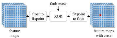
Figure 1: Steps performed by fault injection framework between the computation of two neural network layers Schorn et al. (2019).

4.3 Results

4.3.1 Trade-off analysis between objectives

Table 1: Properties of models that optimize a respective cost dimension. E.g. model BestASI (second row) denotes the optimizer of the ASI objective. Bold numbers indicate minimal values among the selected 50 models with best validation error. Data transfer and accumulated data-computation ratio are calculated taking 8-bit fixed-point quantization of activations and weights into account.

Model	Optimized Quantities						Other Quantities
	Architecture Sensitivity Index ($\times 10^{-3}$)	Validation Set Error Rate (%)	Operations (GOp/Frame)	Data Transfer (MB/Frame)	Acc. Data- Computation Ratio (B/Op)		Normalized Worst Objec- tive Value	Number of Parameters ($\times 10^{6}$)	Test Set Error Rate (%) (32b float)	Test Set Error Rate (%) (8b MaxRange)	Test Set Error Rate (%) (8b MinPQE)
CIFAR-10
WorstASI	8.891	9.20	0.050	0.672	7.279		1.000	0.344	7.31	7.58	7.52
BestASI	0.336	9.16	0.420	2.112	1.422		0.959	1.645	6.95	6.91	6.87
BestValErr	4.267	6.52	0.186	2.381	10.230		0.996	1.489	5.48	5.33	5.41
BestEfficiency	1.750	9.18	0.049	0.665	10.264		1.000	0.337	6.54	6.68	6.61
BestADCR	0.336	9.30	0.429	2.122	1.150		0.993	1.654	6.42	6.57	6.47
BalOpt	0.970	7.56	0.127	1.668	4.241		0.371	1.330	5.72	5.66	5.63
GTSRB
WorstASI	8.120	0.45	0.045	0.478	10.218		1.000	0.101	2.53	2.66	2.64
BestASI	0.109	0.30	0.490	1.220	1.058		0.501	0.865	2.60	2.64	2.60
BestValErr	0.217	0.00	0.966	4.629	4.081		1.000	3.200	0.90	1.08	0.99
BestEfficiency	0.651	0.45	0.012	0.181	1.166		0.600	0.041	1.32	1.41	1.41
BestADCR	0.145	0.12	0.600	3.161	1.048		0.670	2.833	2.50	2.61	2.62
BalOpt	0.326	0.20	0.126	0.676	1.057		0.267	0.513	2.78	2.84	2.81

Table 1 lists the properties of certain DNN architectures $N$ obtained for both benchmarks, CIFAR-10 and GTSRB. The selected models are the ones that minimize each an individual objective function $f_{i}(N)$ (BestASI, BestValErr, BestEfficiency and BestADCR), the model with maximum error sensitivity (WorstASI) as well as the model with lowest normalized worst objective value (see Section 2.3) $\left\lVert\bar{\mathfrak{f}}(N)\right\rVert_{\infty}$, i.e. the balanced optimizer of all objectives (BalOpt). The BestEfficiency models actually minimize both $f_{\mathrm{latency}}(N)$ (i.e. operations) and $f_{\mathrm{energy}}(N)$ (i.e. data transfer). This indicates a correlation between the two quantities. The respective models are also the smallest in terms of weight parameters.

It can be seen in Table 1 that choosing a DNN with minimal cost in one objective often leads to the outcome that at least one other objective is close to its worst value. This is especially the case for CIFAR-10, where $\left\lVert\bar{\mathfrak{f}}(N)\right\rVert_{\infty}$ is $1$ or close to $1$ for all single-objective optimizers, BestASI, BestValErr, BestEfficiency, and BestADCR. The optimal trade-off models (BalOpt), however, come quite close to the ideal point, with normalized distances of $0.371$ (CIFAR-10) and $0.267$ (GTSRB).

Another aspect visible in Table 1 is that 8-bit quantization does not significantly increase test set classification error rates of the models in comparison to the 32-bit float case (in some cases the error is even smaller after quantization). The differences between the MaxRange and MinPQE quantization methods with respect to test error rate are marginal.

The resulting distributions of objective values for all $50$ models that were selected after the optimization with LEMONADE are shown in Figure 2 and Figure 3 for CIFAR-10 and GTSRB, respectively. The sub-figures (a)–(d) each depict the outcomes of $f_{\mathrm{ASI}}(N)$ versus one of the other objective functions. It can be seen that the WorstASI models have comparatively few operations and data transfers. However, the reverse is not always true, since there are models with few operations and data transfers as well as low ASI. In other words, it is possible to have high efficiency and high error resilience at the same time.

Another interesting aspect visible in Figure 2 (d) and Figure 3 (d) is a correlation between ADCR and ASI. Consequently, a low ratio of data transfers to operations is not only beneficial for limiting the required bandwidth of the DNN accelerator, but also helps to reduce error sensitivity. This aspect becomes also apparent in Figure 4. It can be seen that models with more operations typically also require more data transfers. However, the BestASI models have a relatively high number of operations in comparison to their data transfers, as they are located offside the main trend in the scatter plot.

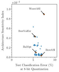
(a)

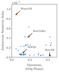
(b)

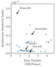
(c)

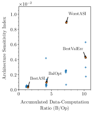
(d)

Figure 2: Pairwise comparison of ASI with each of the other objective function outcomes for 50 Pareto-optimal architectures on CIFAR-10.

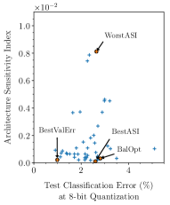
(a)

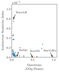
(b)

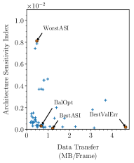
(c)

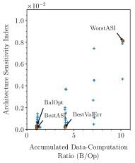
(d)

Figure 3: Pairwise comparison of ASI with each of the other objective function outcomes for 50 Pareto-optimal architectures on GTSRB.

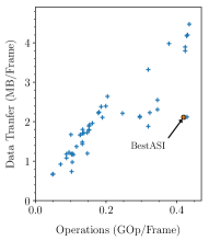
(a)

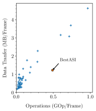
(b)

Figure 4: Data transfer vs. number of operations for Pareto-optimal architectures. BestASI models are located offside the main trend.

4.3.2 Evaluation of resilience prediction

We now evaluate the predictive performance of our ASI metric by performing bit-flip fault injections using the framework described in Section 4.2. Bit-flips are randomly injected in all convolutional layer feature map outputs (after ReLU activation and pooling, where applicable) that are written to memory. MinPQE quantization with 8 bits is used, except where otherwise specified. The value of each bit in the feature map outputs is toggled with a probability given by a defined BER. To get statistically meaningful results Leveugle et al. (2009), random fault locations are sampled $n=200$ times and for each trial the effect on the classification output of the network is measured using the complete test set of the respective benchmark. For this purpose, the CCR, i.e. the fraction of images in the test set that are classified differently after the fault injection, is calculated. The sample mean of CCR over all $n=200$ trials is reported. This can be interpreted as expected probability of SDC at the given BER.

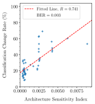
(a)

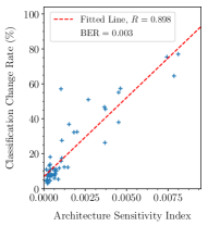
(b)

Figure 5: Correlation of ASI and CCR. A correlation coefficient $R=0.741$ is achieved for CIFAR-10 and $R=0.898$ for GTSRB.

The results of a linear least-squares regression on the ASI versus CCR value pairs of the $50$ optimized models for each benchmark are shown in Figure 5. A BER of 0.003 was used for bit-flip injections. A correlation coefficient $R=0.741$ is achieved for CIFAR-10 and $R=0.898$ for GTSRB. While this indicates that the prediction is not 100% accurate, the correlation is relatively strong. This is especially surprising, considering the fact that ASI is completely determined by the architecture of the neural network and does not require any cumbersome measurements based on test data or weight parameters. Thus, we argue that ASI is an efficient and useful metric to guide NAS towards more resilient DNN architectures.

We also evaluate CCR for varying BER for a subset of models. The results for CIFAR-10 and GTSRB are plotted in Figure 6 and Figure 7, respectively. An approximately linear dependency between BER and CCR can be observed at very low BER. At higher BER a transition first to a rapid growth of CCR (note the log scales) is visible and then the value saturates at a value corresponding to chance probability of choosing the same label after fault injection.

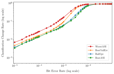
Figure 6: Resulting CCR for different obtained optimizers on CIFAR-10 over a range of BERs.

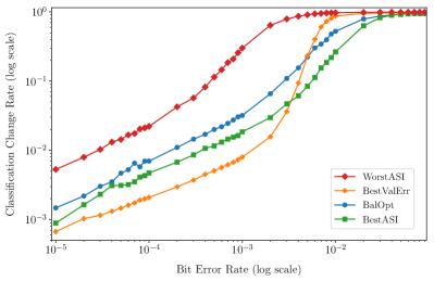
Figure 7: Resulting CCR for different obtained optimizers on GTSRB over a range of BERs.

An interesting finding observable in Figure 6 and Figure 7 is that the BestValErr models exhibit an unexpectedly low CCR at low BER, while they degrade less gracefully (much steeper increase CCR) at high BER. In the case of GTSRB BestValErr is actually, despite its higher ASI, much more resilient than BestASI at low BER. An explanation might be that a good baseline classification performance adds an extra degree of error resilience, which is not captured by ASI. The steeper increase, on the other hand, could be due to an overfitting to the task (i.e. weaker ability for generalization).

4.3.3 Comparison of quantization methods

Finally, we compare the MaxRange and MinPQE quantization methods (see Section 3.3), with respect to resulting CCR after bit-flip fault injections with a BER of 0.005. Results are shown in Figure 8 and Figure 9. The models are sorted in ascending order of CCR after MinPQE quantization in these figures.

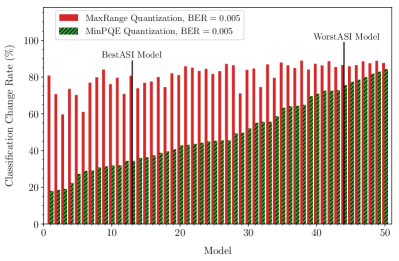
Figure 8: Comparison of CCR at bit error rate 0.005 for CIFAR-10 models quantized with the MaxRange and MinPQE quantization methods. Models sorted after CCR observed with MinPQE quantization.

Figure 9: Comparison of CCR at bit error rate 0.005 for GTSRB models quantized with the MaxRange and MinPQE quantization methods. Models sorted after CCR observed with MinPQE quantization.

It can be seen that MaxRange results in a significantly worse CCR in most of the cases. This can be explained by the fact that MaxRange tends to quantize values to a larger range, which is determined by far outliers, while these outliers are ignored (i.e. clipped) by MinPQE. Consequently, MaxRange leads to a weaker signal-to-noise ratio compared to MinPQE in the case of bit-flip errors. We thus argue that MinPQE is the preferable method, since it achieves both, low baseline classification error rates as well as high error resilience.

5 Conclusions

We have introduced a method for hardware-focused and automated neural architecture design. Our proposed hardware-specific objective functions, which only require network topology information for their evaluation, enable a fast design space exploration and finding of Pareto-optimal solutions of the NAS algorithm. This makes our method efficient and applicable also for more complex classification benchmarks than the ones considered in this paper. We verified the accuracy of resilience prediction with memory bit-flip simulations and found it to be reasonably accurate to guide our NAS algorithm towards architectural resilience optimization. Joint resilience, efficiency, and performance optimization has not been considered in the context of NAS before. Finally, our findings about the influence of different quantization techniques on DNN error resilience highlight the importance of choosing an optimization technique that fosters a high signal-to-noise ratio to limit the influence of bit-flip errors.

References

- Abadi et al. (2015) Abadi M, Agarwal A, Barham P, Brevdo E, Chen Z, Citro C, Corrado GS, Davis A, Dean J, Devin M, Ghemawat S, Goodfellow I, Harp A, Irving G, Isard M, Jia Y, Jozefowicz R, Kaiser L, Kudlur M, Levenberg J, Mane D, Monga R, Moore S, Murray D, Olah C, Schuster M, Shlens J, Steiner B, Sutskever I, Talwar K, Tucker P, Vanhoucke V, Vasudevan V, Viegas F, Vinyals O, Warden P, Wattenberg M, Wicke M, Yu Y, Zheng X (2015) Tensorflow: Large-scale machine learning on heterogeneous distributed systems. URL https://www.tensorflow.org/
- Aitken et al. (2015) Aitken R, Cannon EH, Pant M, Tahoori MB (2015) Resiliency challenges in sub-10nm technologies. In: IEEE 33rd VLSI Test Symposium (VTS), pp 1–4
- Azizimazreah et al. (2018) Azizimazreah A, Gu Y, Gu X, Chen L (2018) Tolerating soft errors in deep learning accelerators with reliable on-chip memory designs. In: IEEE International Conference on Networking, Architecture and Storage (NAS), pp 1–10
- Bach et al. (2015) Bach S, Binder A, Montavon G, Klauschen F, Müller KR, Samek W (2015) On pixel-wise explanations for non-linear classifier decisions by layer-wise relevance propagation. PLOS ONE 10(7):e0130140
- Baker et al. (2017a) Baker B, Gupta O, Naik N, Raskar R (2017a) Designing neural network architectures using reinforcement learning. In: International Conference on Learning Representations
- Baker et al. (2017b) Baker B, Gupta O, Raskar R, Naik N (2017b) Accelerating Neural Architecture Search using Performance Prediction. In: NIPS Workshop on Meta-Learning
- Bender et al. (2018) Bender G, Kindermans PJ, Zoph B, Vasudevan V, Le Q (2018) Understanding and simplifying one-shot architecture search. In: International Conference on Machine Learning
- Blasco et al. (2008) Blasco X, Herrero JM, Sanchis J, Martínez M (2008) A new graphical visualization of n-dimensional Pareto front for decision-making in multiobjective optimization. Information Sciences 178(20):3908–3924
- Cai et al. (2018a) Cai H, Chen T, Zhang W, Yu Y, Wang J (2018a) Efficient architecture search by network transformation. In: AAAI
- Cai et al. (2018b) Cai H, Yang J, Zhang W, Han S, Yu Y (2018b) Path-Level Network Transformation for Efficient Architecture Search. In: International Conference on Machine Learning
- Cai et al. (2019) Cai H, Zhu L, Han S (2019) ProxylessNAS: Direct neural architecture search on target task and hardware. In: International Conference on Learning Representations
- Cai et al. (2018c) Cai L, Barneche AM, Herbout A, Sheng Foo C, Lin J, Ramaseshan Chandrasekhar V, M Sabry M (2018c) TEA-DNN: the quest for time-energy-accuracy co-optimized deep neural networks. arXiv preprint
- Carter et al. (2010) Carter NP, Naeimi H, Gardner DS (2010) Design techniques for cross-layer resilience. In: Design, Automation & Test in Europe Conference & Exhibition (DATE), pp 1023–1028
- Chen et al. (2016) Chen T, Goodfellow IJ, Shlens J (2016) Net2Net: Accelerating learning via knowledge transfer. In: International Conference on Learning Representations
- Chen et al. (2017) Chen YH, Krishna T, Emer JS, Sze V (2017) Eyeriss: An energy-efficient reconfigurable accelerator for deep convolutional neural networks. IEEE Journal of Solid-State Circuits 52(1):127–138
- Cheng et al. (2018) Cheng AC, Dong JD, Hsu CH, Chang SH, Sun M, Chang SC, Pan JY, Chen YT, Wei W, Juan DC (2018) Searching toward Pareto-optimal device-aware neural architectures. In: Proceedings of the International Conference on Computer-Aided Design, ICCAD ’18
- Chenxi et al. (2019) Chenxi L, Liang Chieh C, Florian S, Hartwig A, Wei H, Alan L Y, Li FF (2019) Auto-DeepLab: Hierarchical neural architecture search for semantic image segmentation. In: Conference on Computer Vision and Pattern Recognition
- Chollet (2017) Chollet F (2017) Xception: Deep learning with depthwise separable convolutions. In: IEEE Conference on Computer Vision and Pattern Recognition (CVPR), pp 1800–1807
- Chollet et al. (2015) Chollet F, et al. (2015) Keras. URL https://keras.io
- Deb and Kalyanmoy (2001) Deb K, Kalyanmoy D (2001) Multi-Objective Optimization Using Evolutionary Algorithms. John Wiley & Sons, Inc., New York, NY, USA
- Deb et al. (2000) Deb K, Agrawal S, Pratap A, Meyarivan T (2000) A fast elitist non-dominated sorting genetic algorithm for multi-objective optimization: Nsga-ii. In: Schoenauer M, Deb K, Rudolph G, Yao X, Lutton E, Merelo JJ, Schwefel HP (eds) Parallel Problem Solving from Nature PPSN VI, Springer Berlin Heidelberg, Berlin, Heidelberg, pp 849–858
- Deng et al. (2015) Deng J, Fang Y, Du Z, Wang Y, Li H, Temam O, Ienne P, Novo D, Li X, Chen Y, Wu C (2015) Retraining-based timing error mitigation for hardware neural networks. In: Design, Automation & Test in Europe Conference & Exhibition (DATE), pp 593–596
- DeVries and Taylor (2017) DeVries T, Taylor GW (2017) Improved regularization of convolutional neural networks with cutout. eprint arXiv:1708.04552
- Dias et al. (2010) Dias FM, Borralho R, Fontes P, Antunes A (2010) FTSET: A software tool for fault tolerance evaluation and improvement. Neural Computing and Applications 19(5):701–712
- Dong et al. (2018) Dong JD, Cheng AC, Juan DC, Wei W, Sun M (2018) DPP-Net: Device-aware progressive search for pareto-optimal neural architectures. In: Ferrari V, Hebert M, Sminchisescu C, Weiss Y (eds) Computer Vision – ECCV 2018
- Dreslinski et al. (2010) Dreslinski RG, Wieckowski M, Blaauw D, Sylvester D, Mudge T (2010) Near-threshold computing: Reclaiming Moore’s law through energy efficient integrated circuits. Proceedings of the IEEE 98(2):253–266
- Ehrgott and Tenfelde-Podehl (2003) Ehrgott M, Tenfelde-Podehl D (2003) Computation of ideal and Nadir values and implications for their use in MCDM methods. European Journal of Operational Research 151(1):119–139
- El Mhamdi and Guerraoui (2017) El Mhamdi EM, Guerraoui R (2017) When neurons fail. In: IEEE International Parallel and Distributed Processing Symposium (IPDPS), pp 1028–1037
- Elsken et al. (2017) Elsken T, Metzen JH, Hutter F (2017) Simple And Efficient Architecture Search for Convolutional Neural Networks. In: NIPS Workshop on Meta-Learning
- Elsken et al. (2019a) Elsken T, Metzen JH, Hutter F (2019a) Efficient multi-objective neural architecture search via Lamarckian evolution. In: International Conference on Learning Representations
- Elsken et al. (2019b) Elsken T, Metzen JH, Hutter F (2019b) Neural architecture search: A survey. Journal of Machine Learning Research 20(55):1–21
- Glorot et al. (2011) Glorot X, Bordes A, Bengio Y (2011) Deep sparse rectifier neural networks. In: International Conference on Artificial Intelligence and Statistics (AISTATS), vol 15
- Gomez et al. (2014) Gomez LB, Cappello F, Carro L, DeBardeleben N, Fang B, Gurumurthi S, Pattabiraman K, Rech P, Reorda MS (2014) GPGPUs: How to combine high computational power with high reliability. In: Design, Automation & Test in Europe Conference & Exhibition (DATE)
- Gu et al. (2018) Gu J, Wang Z, Kuen J, Ma L, Shahroudy A, Shuai B, Liu T, Wang X, Wang G, Cai J, Chen T (2018) Recent advances in convolutional neural networks. Pattern Recognition 77:354–377
- He et al. (2016) He K, Zhang X, Ren S, Sun J (2016) Deep residual learning for image recognition. In: IEEE Conference on Computer Vision and Pattern Recognition (CVPR), pp 770–778
- Henkel et al. (2013) Henkel J, Bauer L, Dutt N, Gupta P, Nassif S, Shafique M, Tahoori M, Wehn N (2013) Reliable on-chip systems in the nano-era. In: 50th Annual Design Automation Conference (DAC), pp 695–704
- Hinton et al. (2015) Hinton G, Vinyals O, Dean J (2015) Distilling the knowledge in a neural network. arXiv preprint abs/1503.02531, URL https://arxiv.org/abs/1503.02531, 1503.02531
- Horowitz (2014) Horowitz M (2014) Computing’s energy problem (and what we can do about it). In: IEEE International Solid- State Circuits Conference (ISSCC), pp 10–14
- Hsu et al. (2018) Hsu CH, Chang SH, Juan DC, Pan JY, Chen YT, Wei W, Chang SC (2018) Monas: Multi-objective neural architecture search. arXiv preprint
- Huang et al. (2017) Huang G, Liu Z, van der Maaten L, Weinberger KQ (2017) Densely connected convolutional networks. In: IEEE Conference on Computer Vision and Pattern Recognition (CVPR), pp 4700–4708
- Hutter et al. (2019) Hutter F, Kotthoff L, Vanschoren J (eds) (2019) Automated Machine Learning: Methods, Systems, Challenges. Springer, available at http://automl.org/book.
- Ioffe and Szegedy (2015) Ioffe S, Szegedy C (2015) Batch normalization: Accelerating deep network training by reducing internal covariate shift. In: Proceedings of the 32nd International Conference on Machine Learning
- Jacob et al. (2018) Jacob B, Kligys S, Chen B, Zhu M, Tang M, Howard AG, Adam H, Kalenichenko D (2018) Quantization and training of neural networks for efficient integer-arithmetic-only inference. In: IEEE Conference on Computer Vision and Pattern Recognition (CVPR)
- Kerlirzin and Vallet (1993) Kerlirzin P, Vallet F (1993) Robustness in multilayer perceptrons. Neural Computation 5(3):473–482
- Kim et al. (2018) Kim S, Howe P, Moreau T, Alaghi A, Ceze L, Visvesh S (2018) MATIC: Learning around errors for efficient low-voltage neural network accelerators. In: Design, Automation & Test in Europe Conference & Exhibition (DATE)
- Kim et al. (2017) Kim YH, Reddy B, Yun S, Seo C (2017) NEMO: Neuro-evolution with multiobjective optimization of deep neural network for speed and accuracy. In: ICML’17 AutoML Workshop
- Klein et al. (2017) Klein A, Falkner S, Springenberg JT, Hutter F (2017) Learning curve prediction with Bayesian neural networks. In: International Conference on Learning Representations
- Koopman and Wagner (2016) Koopman P, Wagner M (2016) Challenges in autonomous vehicle testing and validation. SAE International Journal of Transportation Safety 4(1):15–24
- Krizhevsky (2009) Krizhevsky A (2009) Learning multiple layers of features from tiny images. Master Thesis, University of Toronto
- Krogh and Hertz (1991) Krogh A, Hertz JA (1991) A simple weight decay can improve generalization. In: Advances in Neural Information Processing Systems
- LeCun et al. (2015) LeCun Y, Bengio Y, Hinton G (2015) Deep learning. Nature 521(7553):436–444
- Leveugle et al. (2009) Leveugle R, Calvez A, Maistri P, Vanhauwaert P (2009) Statistical fault injection: Quantified error and confidence. In: Design, Automation & Test in Europe Conference & Exhibition (DATE), pp 502–506
- Li et al. (2017) Li G, Hari SKS, Sullivan M, Tsai T, Pattabiraman K, Emer J, Keckler SW (2017) Understanding error propagation in deep learning neural network (DNN) accelerators and applications. In: Proceedings of the International Conference for High Performance Computing, Networking, Storage and Analysis
- Lin et al. (2016) Lin DD, Talathi SS, Annapureddy VS (2016) Fixed point quantization of deep convolutional networks. In: Proceedings of the 33rd International Conference on Machine Learning, vol 48, pp 2849–2858
- Lin et al. (2018) Lin SC, Zhang Y, Hsu CH, Skach M, Haque ME, Tang L, Mars J (2018) The architectural implications of autonomous driving: Constraints and acceleration. In: International Conference on Architectural Support for Programming Languages and Operating Systems, pp 751–766
- Liu et al. (2017) Liu C, Hu M, Strachan JP, Li H (2017) Rescuing memristor-based neuromorphic design with high defects. In: 54th Annual Design Automation Conference (DAC), pp 1–6
- Liu et al. (2018) Liu C, Zoph B, Neumann M, Shlens J, Hua W, Li LJ, Fei-Fei L, Yuille A, Huang J, Murphy K (2018) Progressive Neural Architecture Search. In: European Conference on Computer Vision
- Liu et al. (2019) Liu H, Simonyan K, Yang Y (2019) DARTS: Differentiable architecture search. In: International Conference on Learning Representations
- Loshchilov and Hutter (2017) Loshchilov I, Hutter F (2017) SGDR: Stochastic gradient descent with warm restarts. In: International Conference on Learning Representations (ICLR)
- Lu et al. (2019) Lu Z, Whalen I, Boddeti V, Dhebar Y, Deb K, Goodman E, Banzhaf W (2019) NSGA-net: A multi-objective genetic algorithm for neural architecture search
- Mahdiani et al. (2012) Mahdiani HR, Fakhraie SM, Lucas C (2012) Relaxed fault-tolerant hardware implementation of neural networks in the presence of multiple transient errors. IEEE Transactions on Neural Networks and Learning Systems 23(8):1215–1228
- Marques et al. (2017) Marques J, Andrade J, Falcao G (2017) Unreliable memory operation on a convolutional neural network processor. In: IEEE International Workshop on Signal Processing Systems (SiPS)
- Miettinen (1999) Miettinen K (1999) Nonlinear Multiobjective Optimization. Springer Science & Business Media
- Miikkulainen et al. (2017) Miikkulainen R, Liang J, Meyerson E, Rawal A, Fink D, Francon O, Raju B, Shahrzad H, Navruzyan A, Duffy N, Hodjat B (2017) Evolving Deep Neural Networks. In: arXiv:1703.00548
- Mittal (2016) Mittal S (2016) A survey of techniques for approximate computing. ACM Computing Surveys 48(4):1–33
- Montavon et al. (2017) Montavon G, Lapuschkin S, Binder A, Samek W, Müller KR (2017) Explaining nonlinear classification decisions with deep Taylor decomposition. Pattern Recognition 65:211–222
- Montavon et al. (2018) Montavon G, Samek W, Müller KR (2018) Methods for interpreting and understanding deep neural networks. Digital Signal Processing 73:1–15
- Mutlu (2017) Mutlu O (2017) The RowHammer problem and other issues we may face as memory becomes denser. In: Design, Automation & Test in Europe Conference & Exhibition (DATE)
- Pham et al. (2018) Pham H, Guan MY, Zoph B, Le QV, Dean J (2018) Efficient neural architecture search via parameter sharing. In: International Conference on Machine Learning
- Piuri (2001) Piuri V (2001) Analysis of fault tolerance in artificial neural networks. Journal of Parallel and Distributed Computing 61(1):18–48
- Reagen et al. (2016) Reagen B, Whatmough P, Adolf R, Rama S, Lee H, Lee SK, Hernandez-Lobato JM, Wei GY, Brooks D (2016) Minerva: Enabling low-power, highly-accurate deep neural network accelerators. In: ACM/IEEE 43rd Annual International Symposium on Computer Architecture (ISCA), pp 267–278
- Reagen et al. (2018) Reagen B, Gupta U, Pentecost L, Whatmough P, Lee SK, Mulholland N, Brooks D, Wei GY (2018) Ares: A framework for quantifying the resilience of deep neural networks. In: 55th Annual Design Automation Conference (DAC)
- Real et al. (2017) Real E, Moore S, Selle A, Saxena S, Suematsu YL, Tan J, Le QV, Kurakin A (2017) Large-scale evolution of image classifiers. In: Precup D, Teh YW (eds) Proceedings of the 34th International Conference on Machine Learning, PMLR, International Convention Centre, Sydney, Australia, Proceedings of Machine Learning Research, vol 70, pp 2902–2911
- Real et al. (2019) Real E, Aggarwal A, Huang Y, Le QV (2019) Aging Evolution for Image Classifier Architecture Search. In: AAAI
- Saikia et al. (2019) Saikia T, Marrakchi Y, Zela A, Hutter F, Brox T (2019) Autodispnet: Improving disparity estimation with automl
- Salami et al. (2018) Salami B, Unsal OS, Kestelman AC (2018) On the resilience of RTL NN accelerators: Fault characterization and mitigation. In: 30th International Symposium on Computer Architecture and High Performance Computing (SBAC-PAD), pp 322–329
- Sandler et al. (2018) Sandler M, Howard A, Zhu M, Zhmoginov A, Chen LC (2018) MobileNetV2: Inverted residuals and linear bottlenecks. In: IEEE Conference on Computer Vision and Pattern Recognition (CVPR)
- Santos et al. (2019) Santos FFd, Pimenta PF, Lunardi C, Draghetti L, Carro L, Kaeli D, Rech P (2019) Analyzing and increasing the reliability of convolutional neural networks on GPUs. IEEE Transactions on Reliability 68(2):663–677
- Saxena and Verbeek (2016) Saxena S, Verbeek J (2016) Convolutional neural fabrics. In: Lee DD, Sugiyama M, Luxburg UV, Guyon I, Garnett R (eds) Advances in Neural Information Processing Systems 29, Curran Associates, Inc., pp 4053–4061
- Schorn et al. (2018a) Schorn C, Guntoro A, Ascheid G (2018a) Accurate neuron resilience prediction for a flexible reliability management in neural network accelerators. In: Design, Automation & Test in Europe Conference & Exhibition (DATE)
- Schorn et al. (2018b) Schorn C, Guntoro A, Ascheid G (2018b) Efficient on-line error detection and mitigation for deep neural network accelerators. In: Gallina B, Skavhaug A, Bitsch F (eds) Computer Safety, Reliability, and Security (SAFECOMP), Springer, LNCS, vol 11093
- Schorn et al. (2019) Schorn C, Guntoro A, Ascheid G (2019) An efficient bit-flip resilience optimization method for deep neural networks. In: Design, Automation & Test in Europe Conference & Exhibition (DATE), pp 1486–1491
- Sridharan et al. (2015) Sridharan V, DeBardeleben N, Blanchard S, Ferreira KB, Stearley J, Shalf J, Gurumurthi S (2015) Memory errors in modern systems: The good, the bad, and the ugly. In: Twentieth International Conference on Architectural Support for Programming Languages and Operating Systems (ASPLOS), pp 297–310
- Srinivasan et al. (2016) Srinivasan G, Wijesinghe P, Sarwar SS, Jaiswal A, Roy K (2016) Significance driven hybrid 8T-6T SRAM for energy-efficient synaptic storage in artificial neural networks. In: Design, Automation & Test in Europe Conference & Exhibition (DATE)
- Srivastava et al. (2014) Srivastava N, Hinton GE, Krizhevsky A, Sutskever I, Salakhutdinov RR (2014) Dropout: A simple way to prevent neural networks from overfitting. Journal of Machine Learning Research 15:1929–1958
- Stallkamp et al. (2012) Stallkamp J, Schlipsing M, Salmen J, Igel C (2012) Man vs. computer: Benchmarking machine learning algorithms for traffic sign recognition. Neural Networks 32:323–332
- Stanley and Miikkulainen (2002) Stanley KO, Miikkulainen R (2002) Evolving neural networks through augmenting topologies. Evolutionary Computation 10:99–127
- Sze et al. (2017) Sze V, Chen YH, Yang TJ, Emer JS (2017) Efficient processing of deep neural networks: A tutorial and survey. Proceedings of the IEEE 105(12):2295–2329
- Szegedy et al. (2016) Szegedy C, Vanhoucke V, Ioffe S, Shlens J, Wojna Z (2016) Rethinking the inception architecture for computer vision. In: IEEE Conference on Computer Vision and Pattern Recognition (CVPR), pp 2818–2826
- Tan et al. (2018) Tan M, Chen B, Pang R, Vasudevan V, Le QV (2018) Mnasnet: Platform-aware neural architecture search for mobile. arXiv preprint
- Torres-Huitzil and Girau (2017) Torres-Huitzil C, Girau B (2017) Fault and error tolerance in neural networks: A review. IEEE Access 5:17322–17341
- Vanhoucke et al. (2011) Vanhoucke V, Senior A, Mao MZ (2011) Improving the speed of neural networks on CPUs. In: Deep Learning and Unsupervised Feature Learning Workshop, NIPS 2011
- Venkataramani et al. (2014) Venkataramani S, Ranjan A, Roy K, Raghunathan A (2014) AxNN: Energy-efficient neuromorphic systems using approximate computing. In: IEEE/ACM International Symposium on Low Power Electronics and Design (ISLPED), pp 27–32
- Vogel et al. (2019) Vogel S, Springer J, Guntoro A, Ascheid G (2019) Self-supervised quantization of pre-trained neural networks for multiplierless acceleration. In: Design, Automation & Test in Europe Conference & Exhibition (DATE), pp 1088–1093
- Wei et al. (2016) Wei T, Wang C, Rui Y, Chen CW (2016) Network morphism. In: Balcan MF, Weinberger KQ (eds) Proceedings of The 33rd International Conference on Machine Learning, PMLR, New York, New York, USA, Proceedings of Machine Learning Research, vol 48, pp 564–572
- Whatmough et al. (2018) Whatmough PN, Lee SK, Brooks D, Wei GY (2018) DNN Engine: A 28-nm timing-error tolerant sparse deep neural network processor for IoT applications. IEEE Journal of Solid-State Circuits 53(9):2722–2731
- WikiChip (2019) WikiChip (2019) FSD Chip - Tesla. URL https://en.wikichip.org/wiki/fsd_chip
- Williams et al. (2009) Williams S, Waterman A, Patterson D (2009) Roofline: An insightful visual performance model for multicore architectures. Communications of the ACM 52(4):65–76
- Wu et al. (2019) Wu B, Dai X, Zhang P, Wang Y, Sun F, Wu Y, Tian Y, Vajda P, Jia Y, Keutzer K (2019) FBNet: Hardware-aware efficient convnet design via differentiable neural architecture search. arXiv preprint
- Xia et al. (2017) Xia L, Liu M, Ning X, Chakrabarty K, Wang Y (2017) Fault-tolerant training with on-line fault detection for RRAM-based neural computing systems. In: 54th Annual Design Automation Conference (DAC)
- Xie et al. (2019) Xie S, Zheng H, Liu C, Lin L (2019) SNAS: stochastic neural architecture search. In: International Conference on Learning Representations
- Yang and Murmann (2017) Yang L, Murmann B (2017) SRAM voltage scaling for energy-efficient convolutional neural networks. In: 18th International Symposium on Quality Electronic Design (ISQED), pp 7–12
- Zela et al. (2019) Zela A, Elsken T, Saikia T, Marrakchi Y, Brox T, Hutter F (2019) Understanding and Robustifying Differentiable Architecture Search. arXiv preprint
- Zhang et al. (2018a) Zhang C, Sun G, Fang Z, Zhou P, Pan P, Cong J (2018a) Caffeine: Towards uniformed representation and acceleration for deep convolutional neural networks. IEEE Transactions on Computer-Aided Design of Integrated Circuits and Systems
- Zhang et al. (2018b) Zhang H, Cisse M, Dauphin YN, Lopez-Paz D (2018b) mixup: Beyond empirical risk minimization. In: International Conference on Learning Representations (ICLR)
- Zhang et al. (2015) Zhang Q, Wang T, Tian Y, Yuan F, Xu Q (2015) ApproxANN: An approximate computing framework for artificial neural network. In: Design, Automation & Test in Europe Conference & Exhibition (DATE), pp 701–706
- Zhong et al. (2018) Zhong Z, Yang Z, Deng B, Yan J, Wu W, Shao J, Liu CL (2018) BlockQNN: Efficient block-wise neural network architecture generation. arXiv preprint
- Zoph and Le (2017) Zoph B, Le QV (2017) Neural architecture search with reinforcement learning. In: International Conference on Learning Representations
- Zoph et al. (2018) Zoph B, Vasudevan V, Shlens J, Le QV (2018) Learning transferable architectures for scalable image recognition. In: Conference on Computer Vision and Pattern Recognition