A Darwin Time Domain Scheme for the Simulation of Transient Quasistatic Electromagnetic Fields Including Resistive, Capacitive and Inductive Effects

Abstract

The Darwin field model addresses an approximation to Maxwell’s equations where radiation effects are neglected. It allows to describe general quasistatic electromagnetic field phenomena including inductive, resistive and capacitive effects. A Darwin formulation based on the Darwin-Ampère equation and the implicitly included Darwin-continuity equation yields a non-symmetric and ill-conditioned algebraic systems of equations received from applying a geometric spatial discretization scheme and the implicit backward differentiation time integration method. A two-step solution scheme is presented where the underlying block-Gauss-Seidel method is shown to change the initially chosen gauge condition and the resulting scheme only requires to solve a weakly coupled electro-quasistatic and a magneto-quasistatic discrete field formulation consecutively in each time step. Results of numerical test problems validate the chosen approach.

I Introduction

Quasistatic field models derived from Maxwell’s equations are considered valid, if the shortest wavelength of a problem well exceeds the diameter of the considered problem [1], [2]. In these cases, radiation effects can be neglected. For further taxonomy, the electric energy density $w_{e}$ and magnetic energy density $w_{m}$ are considered: in case of $w_{e}\gg w_{m}$ everywhere in the problem domain, the electro-quasistatic model is applicable and a variation of the magnetic electric can be neglected, i.e., $\frac{\partial}{\partial t}\bf{B}\approx 0.$ Thus, the electric field is irrotational $(\operatorname{curl}\bf{E}=0)$ and governed by resistive and capacitive effects. In case of $w_{e}\ll w_{m},$ the magneto-quasistatic field approximation only takes into account resistive and inductive field effects where displacement currents are neglected within Ampère’s law, i.e., $\frac{\partial}{\partial t}\bf{D}\approx 0.$

Quasistatic field scenarios, where $w_{e}\approx w_{m}$ holds, i.e., where capacitive, resistive and inductive field effects are to be considered in the same problem, are often described using the full set Maxwell’s equations. As a result, in these models the otherwise negligible radiation effects are still considered as an unnecessary part of the model. Especially in time domain formulations this results in a high stiffness of the resulting discrete field formulations. Alternatively, quasistatic models of such scenarios often involve the use of lumped parameter formulations based on Kirchhoff’s equations.

The Darwin field model is an approximation to Maxwell’s equations related to general quasistatic field scenarios including capacitive, resistive and inductive field effects, i.e., where only radiation effects can be neglected [3, 4, 5, 6, 7, 8, 9].

Following the notation in [8], in the quasistatic Darwin field model, the electric field $\bf E$ is subject to a decomposition

$$\bf{E}=\bf{E}_{\mbox{\scriptsize irr.}}+\bf{E}_{\mbox{\scriptsize rem.}},$$ (1)

and split up into an irrotational part $\bf{E}_{\mbox{\scriptsize irr.}}$ with $\operatorname{curl}(\bf{E}_{\mbox{\scriptsize irr.}})=0,$ for which a scalar electric potential representation $\bf{E}_{\mbox{\scriptsize irr.}}=-\operatorname{grad}(\varphi)$ exists, and a remainder part $\bf{E}_{\mbox{\scriptsize rem.}}$ In (1), $\operatorname{div}(\bf{E}_{\mbox{\scriptsize rem.}})=0$ only holds in the uniquely special case of a Helmholtz decomposition that is typically only admissible for homogeneous material distributions. Alternatively, $\operatorname{div}(\bf{E}_{\mbox{\scriptsize rem.}}$) may be nonzero, which needs to be taken into account within an additional gauge. Within the Darwin field model, the rotational parts of the displacement current densities are neglected with $\frac{\partial}{\partial t}(\varepsilon\bf{E}_{\mbox{\scriptsize rot}})=0.$ This essentially eliminates the hyperbolic character of the full Maxwell’s equations which is responsible for modeling wave propagation phenomena and translates the Darwin model into a system with only first order time derivatives. Based on these equations several reformulations in terms of the magnetic vector potential $\bf{A}$ and scalar potential $\varphi$ can be formulated.

Following this introduction, in section II a quasistatic field model for time domain problems is formulated featuring the Darwin-Ampère’s equation and its corresponding Darwin-continuity equation in terms of electrodynamic potentials. Section III describes the space and time discretzation of this Darwin formulation resulting in ill-conditioned and non-symmetric monolithic algebraic systems of equations. Section IV introduces a two-step solution technique which requires only symmetric algebraic systems to be solved. In Section V, numerical test results are shown, including a discussion of the results, followed by a conclusion.

II $(\bf{A},\varphi)$ Formulation for the Darwin Model

The splitting of the electric field in (1) is expressed in terms of electrodynamic potentials, i.e., the magnetic vector potential $\bf{A}$ and the scalar electric potential $\varphi$, with $\bf{E}_{\mbox{\scriptsize rem.}}=-{\frac{\mathrm{\partial}}{\mathrm{\partial}t}}{\bf A}$ and $\bf{E}_{\mbox{\scriptsize irr.}}=-\operatorname{grad}\varphi.$ Initially, the electric field then reads

$$\bf{E}=-{\frac{\mathrm{\partial}}{\mathrm{\partial}t}}{\bf A}-\operatorname{grad}\varphi.$$ (2)

The Darwin formulation ignores the rotational parts of the displacement current densities related to the radiation of electromagnetic waves, i.e., in the electric displacement currents , i.e., $\frac{\mathrm{\partial}^{2}}{\mathrm{\partial}t^{2}}\bf{A}\approx 0.$

With this ansatz, the Ampère’s equation reduces to the Darwin-Ampère’s equation

$$\operatorname{curl}(\nu\operatorname{curl}\bf{A})\!+\!\kappa{\frac{\mathrm{\partial}}{\mathrm{\partial}t}}\bf{A}\!+\!\kappa\operatorname{grad}\varphi\!+\!\varepsilon\operatorname{grad}{\frac{\mathrm{\partial}}{\mathrm{\partial}t}}\varphi\!=\bf{J}_{\mathrm{s}},$$ (3)

where $\nu$ is the reluctivity, $\kappa$ the specific electric conductivity, $\varepsilon$ the permittivity and $\bf{J}_{\mathrm{s}}$ denotes a transient source current density.

For the solution of (3) an additional equation is required to describe the relation of the magnetic vector potential $\bf A$ and the electric scalar potential $\varphi.$ Due to the gauge invariance of the Darwin field model, various Darwin formulations can be derived [4, 8, 9]. If non-homogeneous material distributions need to be considered in the field model, the coupling of $\bf{A}$ and $\varphi$ in (3) by use of the implicitly contained continuity equation appears as an obvious choice. Left application of the divergence operator to the Darwin-Ampère equation (3) yields a Darwin-model continuity equation [7]

$$\mbox{div}\!\left(\!\!\kappa\frac{\partial}{\partial\bf{t}}\bf{A}\!\!+\!\kappa\operatorname{grad}\varphi\!+\!\varepsilon\operatorname{grad}\frac{\partial}{\partial t}\varphi\!\!\right)\!\!\!\!\!\! = \!\!\!\!\!\mbox{div}\bf{J}_{\mathrm{s}}.$$ (4)

It should be noted, that (4) is not identical to the original continuity equation $\operatorname{div}\bf{J}+{\frac{\mathrm{\partial}}{\mathrm{\partial}t}}\rho=0$ related to the full Maxwell model, where $\rho$ is the electric space charge. Including the Gauß’ law, the full Maxwell model continuity equation contains the expression $\varepsilon\frac{\partial^{2}}{\partial t^{2}}\bf(A)$ related to the rotational parts of the displacement currents. These are specifically omitted within the Darwin model.

III A Discrete Darwin Model Formulation

For the general case of non-homogeneous material distributions, a spatial discretization to the equations (3) and (4) is considered following [7]. The application of a mimetic discretization scheme as e.g. the finite integration technique (FIT) [10, 11], Whitney finite element method (WFEM) [12] or the cell method [13] yields the systems of matrix equations

$$\!\!\mbox{\rm\bf C}^{\!\top}{\bf M}_{\nu}\mbox{\rm\bf C}{\rm\bf a}+{\bf M}_{\kappa}\frac{\mathrm{d}}{\mathrm{d}t}{\rm\bf a}+{\bf M}_{\kappa}\rm{\bf G}\boldsymbol{\rm\bf\varphi}+{\bf M}_{\varepsilon}\rm{\bf G}\frac{\mathrm{d}}{\mathrm{d}t}\boldsymbol{\rm\bf\varphi}\!\!\!\!\! = \!\!\!\!\!\!{\rm\bf j}_{\mathrm{s}},$$ (5)

$$\!\!\rm{\bf G}^{\!\top}{\bf M}_{\kappa}\frac{\mathrm{d}}{\mathrm{d}t}{\rm\bf a}+\rm{\bf G}^{\!\top}{\bf M}_{\kappa}\rm{\bf G}\boldsymbol{\rm\bf\varphi}+\rm{\bf G}^{\!\top}{\bf M}_{\varepsilon}\rm{\bf G}\frac{\mathrm{d}}{\mathrm{d}t}\boldsymbol{\rm\bf\varphi}\!\!\!\!\! = \!\!\!\!\!\!\rm{\bf G}^{\!\top}{\rm\bf j}_{\mathrm{s}},$$ (6)

where ${\rm\bf a}$ is the degrees of freedom (dof) vector related to the magnetic vector potential, $\boldsymbol{\rm\bf\varphi}$ is the dof vector of electric nodal scalar potentials, C is the discrete curl operator matrix, $\rm{\bf G}$ and $\rm{\bf G}^{\!\top}$ are discrete gradient and (negative) divergence operator matrices. The matrices ${\bf M}_{\nu},{\bf M}_{\kappa},{\bf M}_{\varepsilon}$ are the (possibly nonlinear) discrete material matrices of reluctivities, conductivities and permittivities, respectively, and the construction of these discrete Hodge operators depends on the specific discretization scheme.

The discrete Darwin equations (5) and (6) can be rewritten as a first order differential-algebraic system of equations

$$\left[\begin{array}[]{cc}{\bf M}_{\kappa}&{\bf M}_{\varepsilon}\rm{\bf G}\\ \rm{\bf G}^{\!\top}{\bf M}_{\kappa}&\rm{\bf G}^{\!\top}{\bf M}_{\varepsilon}\rm{\bf G}\end{array}\right]\frac{\mathrm{d}}{\mathrm{d}t}\left[\begin{array}[]{c}{\rm\bf a}\\ \boldsymbol{\rm\bf\varphi}\end{array}\right]$$ (11)

$$+\left[\begin{array}[]{cc}\mbox{\rm\bf C}^{\!\top}{\bf M}_{\nu}\mbox{\rm\bf C}&{\bf M}_{\kappa}\rm{\bf G}\\ {\mbox{\rm\bf 0}}&\rm{\bf G}^{\!\top}{\bf M}_{\kappa}\rm{\bf G}\end{array}\right]\left[\begin{array}[]{c}{\rm\bf a}\\ \boldsymbol{\rm\bf\varphi}\end{array}\right]=\left[\begin{array}[]{c}{\rm\bf j}_{s}\\ \rm{\bf G}^{\!\top}{\rm\bf j}_{s}\end{array}\right].$$ (18)

While the non-symmetry of the block matrices in (18) can be partially eliminated, the presence of metallic objects in the problem domain will result in large differences in the order of magnitude of the entries.

A time discrete Darwin model based on the monolithic time domain formulation (18) results from the application of e.g. a first order convergent Euler backward differentiation (BDF1) formula [14] with a unconditionally stable time step $\Delta t:=t^{n+1}-t^{n}.$ With ${\bf M}_{\sigma}:={\bf M}_{\kappa}+\frac{1}{\Delta t}{\bf M}_{\varepsilon}$ the implicit time stepping scheme requires to solve the algebraic system of equations

$$\left[\begin{array}[]{cc}\mbox{\rm\bf C}^{\!\top}{\bf M}_{\nu}\mbox{\rm\bf C}+\frac{1}{\Delta t}{\bf M}_{\kappa}&{\bf M}_{\sigma}\rm{\bf G}\\ \frac{1}{\Delta t}\rm{\bf G}^{\!\top}{\bf M}_{\kappa}&\rm{\bf G}^{\!\top}{\bf M}_{\sigma}\rm{\bf G}\end{array}\right]\left[\begin{array}[]{c}{\rm\bf a}\\ \boldsymbol{\rm\bf\varphi}\end{array}\right]^{n+1}$$ (23)

$$\!\!=\!\!\frac{1}{\Delta t}\left[\begin{array}[]{cc}{\bf M}_{\kappa}&{\bf M}_{\varepsilon}\rm{\bf G}\\ \rm{\bf G}^{\!\top}{\bf M}_{\kappa}&\rm{\bf G}^{\!\top}{\bf M}_{\varepsilon}\rm{\bf G}\end{array}\right]\left[\begin{array}[]{c}{\rm\bf a}\\ \boldsymbol{\rm\bf\varphi}\end{array}\right]^{n}+\left[\begin{array}[]{c}{\rm\bf j}_{\mathrm{s}}\\ \rm{\bf G}^{\!\top}{\rm\bf j}_{\mathrm{s}}\end{array}\right]^{n+1}$$ (30)

for each time step and Newton iteration in case on nonlinear material laws. The real-valued system matrix is non-symmetric and can not be symmetrized; it is singular, if ${\bf M}_{\kappa}$ is singular. In [14] the system (30) is additionally regularized assuming a non-physical conductivity in the non-conductive regions of the simulation problem. The system matrices of the monolithic time discrete algebraic systems of equations (30) can be extremely ill-conditioned due to their off-diagonal matrix blocks with entries varying by different orders of magnitude. In [14] a direct solver based on sparse LU-decomposition was used for a discrete problem with a total number of only 12,101 dofs.

IV A Two-Step Darwin Time Domain Scheme

Rewriting the mutually coupled equations (5) and (6) into

$$\!\!\!\!\!\!\!\!\mbox{\rm\bf C}^{\!\top}{\bf M}_{\nu}\mbox{\rm\bf C}{\rm\bf a}\!+\!{\bf M}_{\kappa}\frac{\mathrm{d}}{\mathrm{d}t}{\rm\bf a}\!\!\!\!\! = \!\!\!\!\!{\rm\bf j}_{\mathrm{s}}\!-\!{\bf M}_{\kappa}\rm{\bf G}\boldsymbol{\rm\bf\varphi}\!-\!{\bf M}_{\varepsilon}\rm{\bf G}\frac{\mathrm{d}}{\mathrm{d}t}\boldsymbol{\rm\bf\varphi},$$ (31)

$$\!\!\!\!\!\!\!\!\rm{\bf G}^{\!\top}{\bf M}_{\kappa}\rm{\bf G}\boldsymbol{\rm\bf\varphi}\!+\!\rm{\bf G}^{\!\top}{\bf M}_{\varepsilon}\rm{\bf G}\frac{\mathrm{d}}{\mathrm{d}t}\boldsymbol{\rm\bf\varphi}\!\!\!\!\! = \!\!\!\!\!\rm{\bf G}^{\!\top}{\rm\bf j}_{\mathrm{s}}\!-\!\rm{\bf G}^{\!\top}{\bf M}_{\kappa}\frac{\mathrm{d}}{\mathrm{d}t}{\rm\bf a}$$ (32)

shows both the discrete magneto-quasistatic ($\bf{A}^{\star}$) formulation (31) (see also [15, 16, 17]) and the discrete electro-quasistatic scalar electric potential formulation (32) (see [18]) coupled to each other with their specific right hand side vectors, respectively.

This motivates adopting a strong coupled iteration approach for the solution of the time and space discretized reformulations of (31) and (32). This approach is identical to an iterative block-Gauss-Seidel solution of the monolithic system (30) whose convergence can be shown by inspecting the spectral properties of the matrices.

Let’s denote by ${\rm\bf a}_{m}^{n+1}$ and $\boldsymbol{\rm\bf\varphi}_{m}^{n+1}$ the iterative solution after the $m$-th Gauss-Seidel iteration at time step $n+1$. The iteration scheme requires an initial guess, e.g. by extrapolation

$${\rm\bf a}_{0}^{n+1}:={\rm\bf a}^{n},$$ (33)

where ${\rm\bf a}^{n}$ denotes the final solution at time step $n$, i.e., after $m=1,2,\ldots$ iterations.

Due to discrete conservation properties of the discrete field formulations [11], the discrete divergence relation

$$\rm{\bf G}^{\!\top}{\bf M}_{\kappa}{\rm\bf a}_{m+1}^{n+1}=\rm{\bf G}^{\!\top}{\bf M}_{\kappa}{\rm\bf a}_{m}^{n+1}$$ (34)

holds. When using (33), this discrete conservation property (34) implicitly eliminates the time discrete backward derivative expression $\frac{1}{\Delta t}\rm{\bf G}^{\!\top}{\bf M}_{\kappa}\left[{\rm\bf a}_{m+1}^{n+1}-{\rm\bf a}^{n}\right]$ within the iteration scheme. This translates to $\mbox{div}\!\left(\!\kappa\frac{\partial}{\partial\bf{t}}\bf{A}\!\right)=0$ in the continuous case, i.e., the rotational parts of the eddy current densities will be solenoidal. This is an physically acceptable model assumption in case of highly conductive materials within which the effects of the displacement currents are negligible. Due to this, the Darwin continuity equation (4) reduces to the standard electro-quasistatic field formulation [18].

This property weakens the coupling of (31) and (32) and the iterative scheme reduces to the two-step approach shown in Algorithm 1, where in each time step only two symmetric and positive (semi-)definite systems of algebraic equations need to be solved consecutively. For this task efficient solution schemes are available (see e.g. [17, 18, 19]).

Algorithm 1 Two-Step Darwin Time Domain Algorithm

1:Initialize $\boldsymbol{\rm\bf\varphi}^{0}:=\boldsymbol{\rm\bf\varphi}(t_{0});{\rm\bf a}^{0}:={\rm\bf a}(t_{0});$

2:for $n\leftarrow 0:n_{\mbox{\scriptsize End}}$: do

3:     Solve:

4:     $\left[\rm{\bf G}^{\!\top}{\bf M}_{\sigma}\rm{\bf G}\right]\boldsymbol{\rm\bf\varphi}^{n+1}={\rm{\bf G}}^{\!\top}\!{\rm\bf j}_{s}^{n+1}\!\!+\!\frac{1}{\Delta t}{\rm{\bf G}}^{\!\top}\!{\bf M}_{\varepsilon}{\rm{\bf G}}\boldsymbol{\rm\bf\varphi}^{n};$

5:     Solve:

6:     $\bigl{[}\mbox{\rm\bf C}^{\!\top}{\bf M}_{\nu}\mbox{\rm\bf C}+\frac{1}{\Delta t}{\bf M}_{\kappa}\bigr{]}{\rm\bf a}^{n+1}$

7:     $={\rm\bf j}_{s}^{n+1}+\frac{1}{\Delta t}{\bf M}_{\kappa}{\rm\bf a}^{n}-{\bf M}_{\sigma}{\rm{\bf G}}\boldsymbol{\rm\bf\varphi}^{n+1}+\frac{1}{\Delta t}{\bf M}_{\varepsilon}{\rm{\bf G}}\boldsymbol{\rm\bf\varphi}^{n};$

8:end for

V Numerical Results

Two test structures are excited at $f=100$ MHz, with dimensions small against the wave length, i.e., the quasistatic assumption holds. Using ramped sinusoidal excitations, the two-step Darwin time domain scheme is implemented using the MFEM library [21]. For the solution of the electro-quasistatic system and the weakly coupled magneto-quasistatic systems at each time step, efficient algebraic multigrid (AMG) schemes provided in the PETSc [19] linear algebra solver library are used.

V-A High-frequency coil

A high-frequency coil structure of 63 mm length (see Fig. 1 (left) is considered using a mesh consisting of 237,835 tetrahedra. For the time-domain simulation a ramped sinusoidal excitation profile is used for 10 periods. The dof vector $\boldsymbol{\rm\bf\varphi}$ has dimension 39,038 and the vector ${\rm\bf a}$ has dimension $278,090$. Fig 2 shows results achieved for the magnetic and the electric field after $t=91/f$ and $t=9,251/f$.

Figure 1: Coil geometry (left); RLC structure geometry (right).

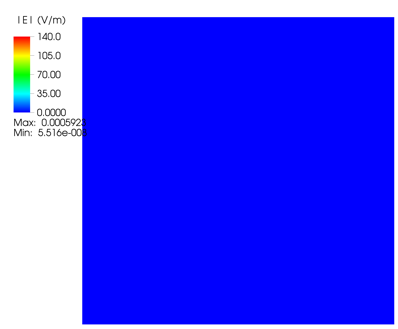
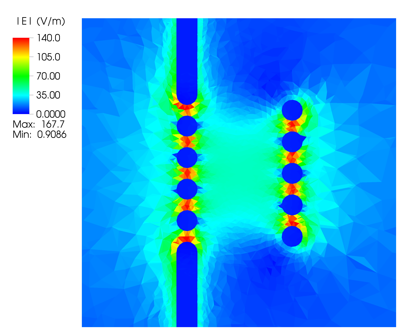
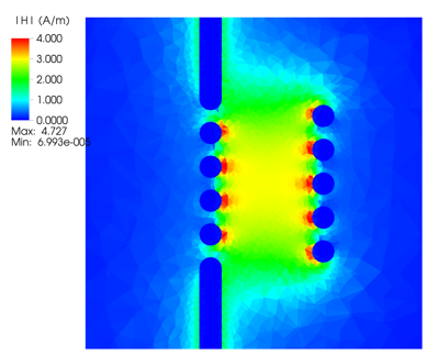
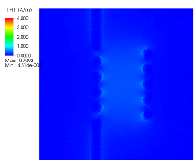
Figure 2: Magnitudes of the electric field $E(t=9T)$ (top left) and magnetic field $B(t=9T)$ (bottom left) and the electric field $E(t=9,25T)$ (top right) and magnetic field $B(t=9.25T)$ (bottom right) simulated with the two-step Darwin time domain algorithm.

V-B RLC Model

A RLC-structure of 63 mm length presented in [20, 9], i.e., a wire (electrical conductivity $\kappa=10^{6}$ S/m connecting a coil and a capacitor with a dielectric inset ($\varepsilon_{r}=2$) (see Fig. 1 (right)) is considered. The FEM mesh consisting of 543,783 tetrahedra. For the time-domain simulation a ramped sinusoidal excitation profile is used for 10 periods. The dof vector $\boldsymbol{\rm\bf\varphi}$ has dimension $88,273$ and the vector ${\rm\bf a}$ has dimension $633,542$. Fig 3 shows the simulation results achieved with the two-step Darwin time domain scheme for the magnetic and the electric field.

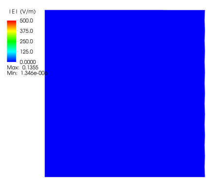
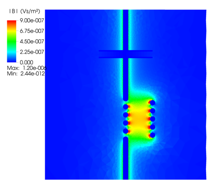
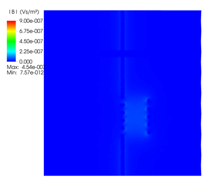
Figure 3: Magnitudes of the electric field $E(t=9T)$ (top left) and magnetic field $B(t=9T)$ (bottom left) and the electric field $E(t=9,25T)$ (top right) and magnetic field $B(t=9.25T)$ (bottom right) simulated with the two-step Darwin time domain algorithm.

V-C Discussion

The simulation results achieved with the two-step time domain method, show that resistive, inductive and capacitive effects are included: The capacitive coupling of the high-frequency coil windings in the HF coil is included with the irrotational parts of the electric field and shown in Fig. 2. The results in Fig. 2 and Fig. 3 show the exchange of electric and magnetic field energy in the sinusoidally excited test structures.

VI Conclusion

The Darwin field model was analyzed to describe general quasistatic electric and magnetic field distributions by only neglecting the rotational contributions of the displacement currents. Starting from an ($\bf{A},\varphi$) formulation of the Darwin-Ampère law and the Darwin-continuity equation, the resulting discrete Darwin model represents a differential-algebraic set of equations. In order to avoid the solution of ill-conditioned and non-symmetric monolithic algebraic systems of equations required within implicit time discretization schemes, a two-step solution schemes was presented based on the consecutive solution of weakly coupled discrete electro- and magneto-quasistatic field formulations in each time step. Numerical results of quasistatic electromagnetic structures, where capacitive, inductive and resistive field effects need to be considered, showed the validity of this two-step approach and its ability to solve realistic 3D problem resolutions by enabling the use of efficient solution schemes.

References

- [1] T. Steinmetz, S. Kurz, and M. Clemens, “Domains of validity of quasistatic and quasistationary field approximations,” COMPEL, vol. 30, no. 5, pp. 1237–1247, 2011.
- [2] V. Mazauric, L. Rondot, and P. Wendling, “Enhancing quasi-static modeling: A claim for electric field computation,” IEEE Trans. Magn., vol. 49, pp. 1629–1632, May 2013.
- [3] P. A. Raviart and E. Sonnendrücker, “A hierarchy of approximate models for the Maxwell equations,” Num. Math., vol. 73, pp. 329 – 372, February 1996.
- [4] J. Larsson, “Electromagnetics from a quasistatic perspective,” Am. J. Phys., vol. 75, no. 3, pp. 230–239, 1995.
- [5] C. Liao and L. Ying, “An analysis of the Darwin model of approximations to Maxwell’s equations in 3-d unbounded domains,” Commun. Math. Sci., vol. 6, no. 3, pp. 695–710, 2008.
- [6] N. Fang, C. Liao, and L. Ying, “Darwin approximation to Maxwell’s equations,” No. I, 2009. ICCS 2009.
- [7] S. Koch, H. Schneider, and T. Weiland, “A low-frequency approximation to the Maxwell equations simultaneously considering inductive and capacitive phenomena,” IEEE Trans. Magn., vol. 48, pp. 511–514, February 2012.
- [8] I. Cortes-Garcia, S. Schöps, H. D. Gersem, and S. Baumanns, “Chapter 1 systems of differential algebraic equations in computational electromagnetics,” in Applications of Differential-Algebraic Equations: Examples and Benchmarks (S. Campell, A. Ilchmann, V. Mehrmann, and T. Reis, eds.), pp. 123–169, Springer Verlag, 2018.
- [9] Z. Badics, S. Bilicz, J. Pávo, and S. Gyimóthy, “Finite element formulations for quasistatic darwin models,” in Proc. CEFC2018 Conference, Hangzhou, China, 2018.
- [10] T. Weiland, “A discretization method for the solution of Maxwell’s equations for six-component fields,” Electronics and Communications AEÜ, vol. 31, no. 3, pp. 116–120, 1977.
- [11] M. Clemens and T. Weiland, “Discrete electromagnetism with the Finite Integration Technique,” in Geometric Methods for Computational Electromagnetics (F. L. Teixeira, ed.), no. 32 in PIER, pp. 65–87, Cambridge, Massachusetts, USA: EMW Publishing, 2001.
- [12] J. C. Nédélec, “Mixed finite elements in ,” Numer. Math., vol. 35, pp. 315–341, 1980.
- [13] E. Tonti, “Finite formulation of the electromagnetic field,” in Geometric Methods for Computational Electromagnetics (F. L. Teixeira, ed.), no. 32 in Progress in Electromagnetic Research (PIER), pp. 1–44, Cambridge, Massachusetts, USA: EMW Publishing, 2001.
- [14] S. Koch and T. Weiland, “Different types of quasistationary formulations for time domain simulations,” Radio Science, vol. 46, no. RS0E12, 2011.
- [15] C. R. I. Emson and J. Simkin, “An optimal method for 3-D eddy currents,” IEEE Trans. Magn., vol. Mag-19, no. 6, pp. 2450–2452, 1983.
- [16] A. Kameari, “Calculation of transient 3d eddy current using edge elements,” IEEE Trans. Magn., vol. 26, no. 5, pp. 466–469, 1990.
- [17] M. Clemens and T. Weiland, “Transient eddy current calculation with the FI-method,” IEEE Trans. Magn., vol. 35, no. 3, pp. 1163–1166, 1999.
- [18] M. Clemens, M. Wilke, G. Benderskaya, H. De Gersem, W. Koch, and T. Weiland, “Transient electro-quasi-static adaptive simulation schemes,” IEEE Trans. Magn., vol. 240, no. 2, pp. 1294–1297, 2004.
- [19] S. Balay, W. D. Gropp, L. C. McInnes, and B. F. Smith, “Efficienct management of parallelism in object oriented numerical software libraries,” in Modern Software Tools in Scientific Computing (E. Arge, A. M. Bruaset, and H. P. Langtangen, eds.), p. 163–202, Birkhauser Press, 1997.
- [20] M. Jochum, O. Farle, and R. Dyczij-Edlinger, “A new low-frequency stable potential formulation for the finite-element simulation of em fields,” IEEE Trans. Magn., vol. 51, no. 3, 2015.
- [21] “Mfem: A modular finite element library.” available via https://mfem.org.