Analysis of an Asymptotic Preserving Low Mach Number Accurate IMEX-RK Scheme for the Wave Equation System

Abstract.

In this paper the analysis of an asymptotic preserving (AP) IMEX-RK finite volume scheme for the wave equation system in the zero Mach number limit is presented. The accuracy of a numerical scheme at low Mach numbers is its ability to maintain the solution close to the incompressible solution for all times, and this can be formulated in terms of the invariance of a space of constant densities and divergence-free velocities. An IMEX-RK methodology is employed to obtain a time semi-discrete scheme, and a space-time fully-discrete scheme is derived by using standard finite volume techniques. The existence of a unique numerical solution, its uniform stability with respect to the Mach number, the AP property, and the accuracy at low Mach numbers are established for both time semi-discrete, and space-time fully-discrete schemes. Extensive numerical case studies confirm uniform second order convergence of the scheme with respect to the Mach number, and all the above-mentioned properties.

1. Introduction

Singular perturbation problems containing small parameters arise in the mathematical modelling of several problems in science and engineering. A typical example of a singularly perturbed problem is the wellknown low Mach number flow in fluid dynamics, often encountered in magnetohydrodynamics, atmospheric, and geophysical flows, weather modelling, combustion theory, and so on. The Euler equations of motion provide a simple yet optimal mathematical tool to model and simulate many of the aforementioned physical processes. The scaled, isentropic Euler equations read

(1.1) $$\partial_{t}\rho+\nabla\cdot(\rho u) =0,$$

$$\partial_{t}(\rho u)+\nabla\cdot(\rho u\otimes u)+\frac{\nabla p}{\varepsilon^{2}} =0,$$

where the independent variables are time $t>0$, and space $x\in\mathbb{R}^{d}$, $d=1,2,3$, and the dependent variables are $\rho=\rho(t,x)>0$, the density, and $u=u(t,x)\in\mathbb{R}^{d}$, the velocity of the fluid.The pressure $p$ is given by the equation of state $p=P(\rho):=\rho^{\gamma}$, where $\gamma$ a constant. Here, $\varepsilon$ is the ratio of a reference fluid velocity to a reference sound velocity, and is known as the reference Mach number. In low Mach number flows, i.e. when $\varepsilon\sim 0$, $\varepsilon$ plays the role of a singular perturbation parameter, and it is wellknown that in the limit $\varepsilon\to 0$, the solutions of (1.1) approximate their incompressible counterparts; see [20] for more details. On the other hand, numerical schemes designed for the system (1.1) suffer from a lot of predicaments in the limit $\varepsilon\to 0$; see, e.g. [21], and the references therein. From a numerical analysis point of view, the main challenges faced by numerical schemes in a low Mach number regime are the stiffness arising due to stringent CFL restrictions, creation of spurious waves, dependence of the numerical viscosity of a scheme on the Mach number leading to lack of stability, and the inability to respect the transitional behaviour of the system of equations in the singular limit.

In our previous work [2], a second order accurate, semi-implicit finite volume approximation for the Euler system (1.1) in a low Mach number regime was proposed and implemented. It is shown that the above mentioned scheme overcomes the severe CFL restrictions, avoids the generation of spurious waves, and is consistent in the singular limit. This paper is aimed to present a rigorous analysis of the semi-implicit scheme of [2] by considering the linear wave equation system as a simplified model. The scaled, purely hyperbolic, linear wave equation system with advection is given by

(1.2) $$\partial_{t}\varrho+(\underline{u}\cdot\nabla)\varrho+\frac{\underline{a}}{\varepsilon}\nabla\cdot u =0,$$

$$\partial_{t}u+(\underline{u}\cdot\nabla)u+\frac{\underline{a}}{\varepsilon}\nabla\varrho =0.$$

Here, $\varrho$ denotes a scaled density with $\rho(t,x)=\underline{\rho}\left(1+\frac{\varepsilon}{\underline{a}}\varrho(t,x)\right)$, and the constants $\underline{\rho},\underline{u}$, and $\underline{a}$ are, respectively, the linearisation states of $\rho,u$ and the sound velocity $a$.

Expanding all the dependent variables in (1.2) using the ansatz

(1.3) $$f(t,x)=f_{(0)}(t,x)+\varepsilon f_{(1)}(t,x)+\varepsilon^{2}f_{(2)}(t,x)+\ldots,$$

and performing a scale analysis with the use of appropriate boundary conditions yields the following linearised, mixed hyperbolic-elliptic, incompressible system:

(1.4) $$\varrho_{(0)} =\mathrm{const.},$$

$$\partial_{t}u_{(0)}+(\underline{u}\cdot\nabla)u_{(0)}+\underline{a}\nabla\varrho_{(1)} =0,$$

$$\nabla\cdot u_{(0)} =0$$

for the unknowns $u_{(0)}$ and $\varrho_{(1)}$.

It is essential for a discretisation of (1.2) to respect the limiting system (1.4) in the asymptotic limit $\varepsilon\to 0$. In addition, it is desirable that its stability restrictions are independent of $\varepsilon$ so that the stiffness arising when $\varepsilon\to 0$ can be overcome. These two requirements fall under the purview of the so-called asymptotic preserving (AP) methodology [9, 17, 18]. In a related work [10], the authors study a strongly anisotropic singular elliptic problem arising in plasma physics. In the singular limit, i.e. when the anisotropy parameter goes to zero, the problem converges to an ill-posed one. As a cure, the authors propose an AP reformulation of the given anisotropic equation in order to write the original problem in such a way that a continuous transition towards the limit can be achieved. Hence, the AP methodology can also help to get rid of the possible ill-posedness which might arise in the singular limit.

It is well known that being AP is predominantly dictated by the particular time discretisation chosen. The scheme designed in [2] makes use of the implicit explicit Runge-Kutta (IMEX-RK) time discretisation and an appropriate flux decomposition to achieve the AP property for the Euler system (1.1) in the zero Mach number limit; see [3, 5, 8, 11, 22, 23, 24, 27] for more detailed discussions on IMEX-RK schemes, AP schemes, and their other applications. As mentioned in the beginning, compressible flow solvers suffer from severe loss of accuracy at low Mach numbers due to the creation of spurious waves. Recently, a detailed analysis was carried out by Dellacherie in [12] on the behaviour of explicit Godunov-type schemes in a low Mach number regime. The above mentioned study using the linear wave equation system (1.2) reveals that the inaccuracies can be avoided by enforcing the particular scheme to preserve a space of constant densities and divergence-free velocities, known as the well-prepared space. Following this, in [2], a scheme which leaves the well-prepared space invariant is designated as asymptotically accurate (AA).

The goal of the current paper is to present a detailed analysis of a time semi-discrete as well as space-time fully-discrete IMEX-RK scheme for the wave equation system (1.2) under the low Mach number scaling. The study focusses on addressing the following three issues:

1. the existence of a unique numerical solution for a fixed $\varepsilon>0$;

2. the uniform stability of the numerical solution with respect to $\varepsilon$, and the AP property;

3. the invariance of the well-prepared space by the numerical solution implying asymptotic accuracy.

The time semi-discrete scheme corresponds to the dual formulation of an elliptic equation for the density, and the existence and uniqueness of its solution is obtained via the saddle point theory of variational problems. The asymptotic consistency, as done, e.g. in [2], then reveals that we do not encounter pathologies, such as ill-posedness of the limit problem, cf. [10]. The fully-discrete scheme obtained by simple central differencing involves circulant matrices [13]. We exploit the theory of these matrices to establish the above properties for the fully-discrete setup.

In order to carry out the analysis, the linear wave equation system (1.2) is rewritten in the evolution form

(1.5) $$\partial_{t}U+H(U)+\frac{1}{\varepsilon}L(U)=0,$$

via the operators $H$ and $L$ defined as

(1.6) $$U:=\begin{pmatrix}\varrho\\ u\end{pmatrix},\ H(U):=\begin{pmatrix}\underline{u}\cdot\nabla\varrho\\ (\underline{u}\cdot\nabla)u\end{pmatrix},\ \mbox{and}\ L(U):=\begin{pmatrix}\underline{a}\nabla\cdot u\\ \underline{a}\nabla\varrho\end{pmatrix}.$$

Here, $H$ is the convective operator with a timescale of order $1$ and $L/\varepsilon$ is the acoustic operator with a timescale of the order of $\varepsilon$. As discussed above, when $\varepsilon\to 0$, the solutions $U=(\varrho,u)$ of (1.6) converge to $U_{(0)}=(\varrho_{(0)},u_{(0)})$ in the well-prepared space, which happens to be the kernel of the operator $L$. Hence, as done in [12], throughout this paper, we restrict our analysis to the following initial value problem:

(1.7) $$\partial_{t}U+\frac{1}{\varepsilon}L(U) =0,$$

$$U(0,x) =U_{0}(x),\ x\in\mathbb{T}^{d},$$

where $\mathbb{T}^{d}$ denotes the $d$-dimensional torus to take into account of the periodic boundary conditions. However, the numerical case studies are performed also on the model (1.5) with advection.

The rest of this paper is organised in the following way. In Section 2 we briefly recall the results from [12], which are relevant for the present study. Section 3 is devoted to a short presentation of IMEX-RK time discretisation for stiff systems of ODEs, and the notions of AP and AA properties. The analysis of the time semi-discrete scheme obtained after employing the IMEX-RK method is taken up in Section 4, where we prove the desired properties mentioned above in (1)-(3). In Section 5 we present a space-time fully-discrete scheme derived by using a finite volume technique. The theory of circulant matrices is used to establish the same properties (1)-(3) for the fully-discrete scheme. The results of numerical case studies are reported in Section 6, where we numerically corroborate the theoretical claims. Finally, the paper is concluded with some remarks in Section 7.

2. Analysis of the Wave Equation System

In this section, we briefly recall some of the results from [12], regarding the low Mach number limit of the wave equation system (1.5). First, we consider the space of solutions of (1.5) which is the Hilbert space of square integrable functions $L^{2}(\mathbb{T}^{d})^{1+d}$. The space $L^{2}(\mathbb{T}^{d})^{1+d}$ is equipped with the innerproduct

(2.1) $$(U_{1},U_{2}):=(\varrho_{1},\varrho_{2})+(u_{1},u_{2}),$$

where $U_{m}=(\varrho_{m},u_{m}),m=1,2$, in the above, and throughout the rest of this paper, $(\cdot,\cdot)$ denotes the $L^{2}$ innerproduct. The kernel of the wave operator $L$ is given by

(2.2) $${\mathcal{E}}:=\left\{U\in L^{2}(\mathbb{T}^{d})^{1+d}\colon\nabla\varrho=0,\ \text{and}\ \nabla\cdot u=0\right\},$$

which is the so-called well-prepared, incompressible, space of constant densities and divergence-free velocities. The orthogonal complement $\tilde{\mathcal{E}}$ of $\mathcal{E}$ is defined as

(2.3) $$\tilde{\mathcal{E}}:=\left\{U\in L^{2}(\mathbb{T}^{d})^{1+d}\colon\int_{\mathbb{T}^{d}}\rho dx=0,\ \text{and}\ \nabla\times u=0\right\}.$$

The spaces $\mathcal{E}$ and $\tilde{\mathcal{E}}$, given by (2.2) and (2.3), yields the following Helmholtz-Hodge-Leray decomposition of $L^{2}(\mathbb{T}^{d})^{1+d}$:

(2.4) $$\mathcal{E}\oplus\tilde{\mathcal{E}}=L^{2}(\mathbb{T}^{d})^{1+d},\ \mbox{and }\ \mathcal{E}\perp\tilde{\mathcal{E}}.$$

As a consequence of (2.4), we can decompose any $U\in L^{2}(\mathbb{T}^{d})^{1+d}$; there exists a unique $\hat{U}\in\mathcal{E}$ and $\tilde{U}\in\tilde{\mathcal{E}}$, such that $U=\hat{U}+\tilde{U}$. We define the Helmholtz-Hodge-Leray projection $\mathbb{P}\colon L^{2}(\mathbb{T}^{d})^{1+d}\to\mathcal{E}$, via

(2.5) $$\mathbb{P}U:=\hat{U}.$$

Definition 2.1.

The energy $E$ of the system (1.2) is defined as

(2.6) $$E:=\frac{1}{2}(U,U).$$

Proposition 2.2.

Let U be a solution of the system (1.2) on $\mathbb{T}^{d}$. Then, the energy $E$ introduced in Definition 2.1 is preserved, i.e.

(2.7) $$E(t)=E(0),\ \text{for all}\ t>0.$$

Remark 2.3.

Proposition 2.2 states that the linear wave equation system (1.2) conserves the energy (2.1).

Proposition 2.4.

Let $U$ be the solution of the system (1.2) with initial data $U_{0}$. Then,

• for all $U_{0}\in\mathcal{E}$, we have $U(t,\cdot)\in\mathcal{E}$ for all $t>0$;

• for all $U_{0}\in\tilde{\mathcal{E}}$, we have $U(t,\cdot)\in\tilde{\mathcal{E}}$ for all $t>0$.

Remark 2.5.

Proposition 2.4 states that the wave equation system leaves both the spaces $\mathcal{E}$ and $\tilde{\mathcal{E}}$ invariant. In other words, if the solution lives in one of these spaces initially, then it lives there for all times.

Theorem 2.6 ([12]).

Let $U$ be a solution of the IVP:

(2.8) $$\partial_{t}U+H(U)+\frac{1}{\varepsilon}L(U) =0,\ t>0,\ x\in\mathbb{T}^{d},$$

(2.9) $$U(0,x) =U_{0}(x),\ x\in\mathbb{T}^{d},$$

and let $\bar{U}$ be a solution of the IVP:

(2.10) $$\partial_{t}\bar{U}+H(\bar{U}) =0,\ t>0,\ x\in\mathbb{T}^{d},$$

(2.11) $$\bar{U}(0,x) =\hat{U}_{0}(x),\ x\in\mathbb{T}^{d},$$

where $\hat{U}_{0}:=\mathbb{P}U_{0}$. Let $U=\hat{U}+\tilde{U}$ be the Helmholtz-Hodge-Leray decomposition of $U$. Then, the following holds.

1. $\hat{U}=\bar{U}$,

2. $\tilde{U}$ is the solution of (2.8) with initial condition $\tilde{U}_{0}:=(\mathbb{I}-\mathbb{P})U_{0}$.

Moreover, there holds the energy conservation:

(2.12) $$E_{in}(t)=E_{in}(0)\ \text{and}\ E_{ac}(t)=E_{ac}(0),\ \text{for all}\ t>0,$$

where $E_{in}:=(\hat{U},\hat{U})$ and $E_{ac}:=(\tilde{U},\tilde{U})$. As a consequence, the following estimate holds:

(2.13) $$\lVert U_{0}-\mathbb{P}U_{0}\rVert=\mathcal{O}(\varepsilon)\implies\lVert U(t)-\mathbb{P}U(t)\rVert=\mathcal{O}(\varepsilon)\ \mbox{for all}\ t>0.$$

Proposition 2.6 lies at the core of the analysis of numerical schemes presented in [12]. Depending on the order of accuracy, numerical schemes introduce numerical diffusion, dispersion or higher order correction terms in the modified partial differential equations (MPDE). However, we desire that the numerical solutions which satisfy the MPDE also exhibit properties close to those of the solutions of the continuous system. One of the key properties is to satisfy the estimate (2.13) which states that a solution remains close to $\mathcal{E}$ for all times $t>0$ if it is so at time $t=0$. The following proposition guarantees a sufficient condition to ensure (2.13), which also accommodates any general linear discretisation.

Proposition 2.7.

[12] Let $U$ be a solution of the IVP:

(2.14) $$\partial_{t}U+\mathcal{F}_{x}U =0,\ t>0,\ x\in\mathbb{T}^{d},$$

(2.15) $$U(0,x) =U_{0}(x),\ x\in\mathbb{T}^{d},$$

which is assumed to be well-posed in $L^{\infty}\left([0,\infty);L^{2}(\mathbb{T}^{d})^{1+d}\right)$, with $\mathcal{F}_{x}$ a linear spatial differential operator. Then the following conclusions hold.

1. The solution $U$ satisfies the estimate

   (2.16) $$\lVert U_{0}-\mathbb{P}U_{0}\rVert=\mathcal{O}(\varepsilon)\implies\lVert U(t)-\bar{U}(t)\rVert=\mathcal{O}(\varepsilon),\ \text{for all}\ t>0,$$

   where $\bar{U}$ is a solution of (2.14) with the initial condition $\bar{U}(0)=\mathbb{P}U_{0}$. However, we don’t have the apriori estimate $\lVert U(t)-\mathbb{P}U(t)\rVert=\mathcal{O}(\varepsilon)$ for all $t>0$.

2. When the operator $\mathcal{F}_{x}$ leaves $\mathcal{E}$ invariant, i.e. whenever $U_{0}\in\mathcal{E}$ implies $U(t)\in\mathcal{E}$ for all $t>0$, then $U$ satisfies the estimate (2.16), and in addition we have

   (2.17) $$\lVert U_{0}-\mathbb{P}U_{0}\rVert=\mathcal{O}(\varepsilon)\implies\lVert U(t)-\mathbb{P}U(t)\rVert=\mathcal{O}(\varepsilon)\ \text{for all}\ t>0.$$

Remark 2.8.

The second part of the above Proposition  2.7 give us the importance of $\mathcal{E}$ invariance for any numerical scheme. It states that if a scheme is $\mathcal{E}$-invariant, then if the initial data $U_{0}$ is almost in the well-prepared subspace $\mathcal{E}$, the solution at all later times also lives close $\mathcal{E}$. Loosely speaking, the estimate (2.17) states that if the initial data is almost incompressible, then the solution for all time $t>0$ is also almost incompressible. It was observed in [12] that satisfying the condition (2.17) avoids the creation of spurious acoustic waves in the numerical solution. Our numerical experiments reported in Section 6 clearly validate this observation.

3. Asymptotic Preserving and Asymptotically Accurate IMEX-RK Schemes

We devote this section to recall the notions of AP and AA schemes as done in [2]. Further, in a nutshell, we review the wellknown IMEX-RK schemes for stiff systems of ODEs which are employed to approximate the time derivatives in system (1.2).

3.1. Asymptotic Preserving Property

One of the essential properties of a numerical approximation for a singular perturbation problem is its ability to capture the solution of the limit system as well as the solution of the original problem. The AP methodology not only provides a framework to address the convergence of the numerical solution to that of the limit system but also takes care of the stability restrictions such that they don’t deteriorate in the singular limit.

Definition 3.1.

Let $\mathcal{P}^{\varepsilon}$ denote a singularly perturbed problem with the perturbation parameter $\varepsilon$. Let $\mathcal{P}^{0}$ denote the limiting system of $\mathcal{P}^{\varepsilon}$ for $\varepsilon\to 0$. A discretisation $\mathcal{P}_{h}^{\varepsilon}$ of $\mathcal{P^{\varepsilon}}$, with $h$ being the discretisation parameter, is called AP, if

1. $\mathcal{P}^{0}_{h}$ is a consistent discretisation of the problem $\mathcal{P}^{0}$, called the asymptotic consistency, and

2. the stability constraints on $h$ are independent of $\varepsilon$, called the asymptotic stability.

In other words, the following diagram commutes:

$$\begin{CD}\mathcal{P}^{\varepsilon}_{h}@>{h\to 0}>{}>\mathcal{P}^{\varepsilon}\\ @V{}V{\varepsilon\to 0}V@V{}V{\varepsilon\to 0}V\\ \mathcal{P}^{0}_{h}@>{h\to 0}>{}>\mathcal{P}^{0}\end{CD}$$

3.2. Asymptotic Accuracy

We note from Proposition 2.4 that a solution of the wave equation system lives in $\mathcal{E}$ at all times if the initial data is taken from $\mathcal{E}$. It was shown in [12] that a sufficient condition for a numerical scheme for the wave equation system to be accurate at low Mach numbers, i.e. it is free from the creation of spurious waves, is the $\mathcal{E}$-invariance. Based on this idea, in [2], the notion of asymptotic accuracy is defined as the following.

Definition 3.2.

A numerical approximation for the wave equation system (1.2) is said to be asymptotically accurate (AA), if it leaves the incompressible subspace $\mathcal{E}$ invariant.

3.3. IMEX-RK Time Discretisation

IMEX-RK schemes provide a robust and efficient framework to design AP schemes for singular perturbation problems. In this work, we only consider a subclass of the IMEX-RK schemes, namely diagonally implicit or (DIRK) schemes. An $s$-stage IMEX-RK scheme is characterised by the two $s\times s$ lower triangular matrices $\tilde{A}=(\tilde{a}_{i,j})$, and $A=(a_{i,j})$, the coefficients $\tilde{c}=(\tilde{c}_{1},\tilde{c}_{2},\ldots,\tilde{c}_{s})$ and $c=(c_{1},c_{2},\ldots,c_{s})$, and the weights $\tilde{\omega}=(\tilde{\omega}_{1},\tilde{\omega}_{2},\ldots,\tilde{\omega}_{s})$ and $\omega=(\omega_{1},\omega_{2},\ldots,\omega_{s})$. Here, the entries of $\tilde{A}$ and $A$ satisfy the conditions $\tilde{a}_{i,j}=0$ for $j\geq i$, and $a_{i,j}=0$ for $j>i$. Let us consider the following stiff system of ODEs in an additive form:

(3.1) $$y^{\prime}=f(t,y)+\frac{1}{\varepsilon}g(t,y),$$

where $0<\varepsilon\ll 1$ is called the stiffness parameter. The functions $f$ and $g$ are known as, respectively, the non-stiff part and the stiff part of the system (3.1); see, e.g. [14], for a comprehensive treatment of such systems.

Let $y^{n}$ be a numerical solution of (3.1) at time $t^{n}$ and let $\Delta t$ denote a fixed timestep. An $s$-stage IMEX-RK scheme, cf., e.g. [3, 23], updates $y^{n}$ to $y^{n+1}$ through $s$ intermediate stages:

(3.2) $$Y_{i} =y^{n}+\Delta t\sum\limits_{j=1}^{i-1}\tilde{a}_{i,j}f(t^{n}+\tilde{c}_{j}\Delta t,Y_{j})+\Delta t\sum\limits_{j=1}^{s}a_{i,j}\frac{1}{\varepsilon}g(t^{n}+c_{j}\Delta t,Y_{j}),\ 1\leq i\leq s,$$

(3.3) $$y^{n+1} =y^{n}+\Delta t\sum\limits_{i=1}^{s}\tilde{\omega}_{i}f(t^{n}+\tilde{c}_{i}\Delta t,Y_{i})+\Delta t\sum\limits_{i=1}^{s}\omega_{i}\frac{1}{\varepsilon}g(t^{n}+c_{i}\Delta t,Y_{i}).$$

In order to further simplify the analysis of the schemes presented in this paper, we restrict ourselves only to two types of DIRK schemes, namely the type-A and type-CK schemes which are defined below; see [19] for details.

Definition 3.3.

An IMEX-RK scheme is said to be of

• type-A, if the matrix $A$ is invertible;

• type-CK, if the matrix $A\in\mathbb{R}^{s\times s},\ s\geq 2$, can be written as

  $$A=\begin{pmatrix}0&0\\ \alpha&A_{s-1}\end{pmatrix},$$

  where $\alpha\in\mathbb{R}^{s-1}$ and $A_{s-1}\in\mathbb{R}^{s-1\times s-1}$ is invertible.

The results presented in later sections, are obtained using both the first order Euler(1,1,1), and second order ARS(2,2,2) schemes for time discretisations; see [23, 24] for their definitions. Here, in the triplet $(s,\sigma,p)$, $s$ is the number of stages of the implicit part, the number $\sigma$ gives the number of stages for the explicit part and $p$ gives the overall order of the scheme. We refer the interested reader to [14, 19, 23, 24] and the references therein for a detailed study of IMEX-RK schemes.

Hypothesis 3.4.

We suppose that the IMEX-RK scheme under consideration is of Type-A or Type CK.

4. Time Semi-discrete Scheme and Its Analysis

In this section we present our time semi-discrete scheme for the wave equation system (1.2) obtained after approximation of the time derivatives using the IMEX-RK methodology described in Section 3. We carry out a detailed analysis of the scheme, and show some if its key properties, namely its solvability, i.e. the existence of a numerical solution for any fixed $\varepsilon>0$, the AP property and the asymptotic accuracy.

4.1. Time Semi-discrete Scheme

As a first step in defining a time semi-discrete scheme, we split the fluxes in (1.2) into a stiff and a non-stiff part, yielding

(4.1) $$G(U):=\frac{\underline{a}}{\varepsilon}\begin{pmatrix}u\\ \varrho\end{pmatrix},\ F(U):=\begin{pmatrix}\varrho\underline{u}\\ \underline{u}\otimes u\end{pmatrix}.$$

Let $0<t^{1}<t^{2}<\cdots<t^{n}<\cdots$ be an increasing sequence of times. In the following, $f^{n}$ denotes an approximation to the value of a function $f(t,x)$ at time $t^{n}$, i.e. $f^{n}(x)\sim f(t^{n},x)$. Treating $F$ explicitly, and $G$ implicitly, the IMEX-RK time semi-discrete scheme can be obtained as follows.

Definition 4.1.

Given an approximation $(\varrho^{n},u^{n})$ of the numerical solution at time $t^{n}$, and a timestep $\Delta t$, the $k^{th}$ stage of an $s$-stage IMEX-RK scheme for the wave equation system (1.2) is defined by

(4.2) $$\varrho^{k} =\varrho^{n}-\Delta t\tilde{a}_{k,\ell}(\underline{u}\cdot\nabla)\varrho^{\ell}-\Delta ta_{k,l}\frac{\underline{a}}{\varepsilon}\nabla\cdot u^{l},\ \mbox{for each}\ k=1,2,\ldots,s,$$

(4.3) $$u^{k} =u^{n}-\Delta t\tilde{a}_{k,\ell}(\underline{u}\cdot\nabla)u^{\ell}-\Delta ta_{k,l}\frac{\underline{a}}{\varepsilon}\nabla\varrho^{l},\ \mbox{for each}\ k=1,2,\ldots,s.$$

The approximate numerical solutions $\varrho^{n+1}$ and $u^{n+1}$ at time $t^{n+1}$ are defined as

(4.4) $$\varrho^{n+1} =\varrho^{n}-\Delta t\tilde{\omega}_{k}(\underline{u}\cdot\nabla)\varrho^{k}-\Delta t\omega_{k}\frac{\underline{a}}{\varepsilon}\nabla\cdot u^{k},$$

(4.5) $$u^{n+1} =u^{n}-\Delta t\tilde{\omega}_{k}(\underline{u}\cdot\nabla)u^{k}-\Delta t\omega_{k}\frac{\underline{a}}{\varepsilon}\nabla\varrho^{k}.$$

In the above, and throughout the rest of this paper, we follow the convention that a repeated index always denotes the summation with respect to that index. Here, the index $k$ assumes values in $\{1,2,\ldots,s\}$, and the indices $\ell$ and $l$ are used to denote, respectively, the summation in the explicit and implicit terms, i.e. they assume values in the sets $\{1,2,\ldots,k-1\}$ and $\{1,2,\ldots,k\}$.

4.2. Solvability of the Time Semi-discrete Scheme

The aim of this subsection is to establish the existence of a numerical solution to (4.2)-(4.5) using variational formulations, and classical saddle point theory; see, e.g. [6, 7] for more details. To this end, let us consider the standard function spaces

(4.6) $$V:=H(\mathrm{div};\mathbb{T}^{d}),\ \mbox{and}\ M:=L^{2}(\mathbb{T}^{d}).$$

In (4.2)-(4.5), we multiply the density updates by a test function $\lambda\in M$ and the velocity updates by a test function $v\in V$, and integrate by parts to get the following weak formulation.

For $k=1,2,\ldots,s$, find $(u^{k},\varrho^{k})\in V\times M$ satisfying

(4.7) $$(u^{k},v)-\Delta ta_{k,k}\frac{\underline{a}}{\varepsilon}(\nabla\cdot v,\varrho^{k}) =(u^{n},v)+\Delta ta_{k,\ell}\frac{\underline{a}}{\varepsilon}(\nabla\cdot v,\varrho^{\ell}),\ \mbox{for all}\ v\in V,$$

(4.8) $$-\Delta ta_{k,k}\frac{\underline{a}}{\varepsilon}(\nabla\cdot u^{k},\lambda)-(\varrho^{k},\lambda) =-(\varrho^{n},\lambda)+\Delta ta_{k,\ell}\frac{\underline{a}}{\varepsilon}(\nabla\cdot u^{\ell},\lambda),\ \mbox{for all}\ \lambda\in M.$$

Finally, find $(u^{n+1},\varrho^{n+1})\in V\times M$ satisfying

(4.9) $$(u^{n+1},v) =(u^{n},v)+\Delta t\omega_{k}\frac{\underline{a}}{\varepsilon}(\nabla\cdot v,\varrho^{k}),\ \mbox{for all}\ v\in V,$$

(4.10) $$(\varrho^{n+1},\lambda) =(\varrho^{n},\lambda)-\Delta t\omega_{k}\frac{\underline{a}}{\varepsilon}(\nabla\cdot u^{k},\lambda),\ \mbox{for all}\ \lambda\in M.$$

Note that the semi-discrete scheme (4.2)-(4.5) admits a solution if, and only if, the weak formulations (4.7)-(4.10) admit a solution.

Theorem 4.2.

Suppose an approximation $(u^{n},\varrho^{n})\in V\times M$ of the numerical solution at time $t^{n}$, and a timestep $\Delta t$ are chosen. Then, under the Hypothesis 3.4, the weak formulations (4.7)-(4.8) are uniquely solvable for a $(u^{k},\varrho^{k})\in V\times M$ for $k=1,2,\ldots,s$. Consequently, (4.9)-(4.10) defines uniquely an approximate numerical solution $(u^{n+1},\varrho^{n+1})\in V\times M$ at time $t^{n+1}=t^{n}+\Delta t$.

The weak formulations (4.7)-(4.8) can be recast in the saddle point form: find $(u^{k},\varrho^{k})\in V\times M$ satisfying

(4.11) $$a_{k}(u^{k},v)+b_{k}(v,\varrho^{k}) =l_{k}(v),\ \mbox{for all}\ v\in V,$$

$$b_{k}(u^{k},\lambda)-c_{k}(\varrho^{k},\lambda) =\chi_{k}(\lambda),\ \mbox{for all}\ \lambda\in M.$$

Here, the bilinear forms $a_{k}\colon V\times V\to\mathbb{R}$, $b_{k}\colon V\times M\to\mathbb{R}$, and $c_{k}\colon M\times M\to\mathbb{R}$ are defined as

(4.12) $$a_{k}(v,w) :=(v,w),\ \mbox{for each}\ v,w\ \in V,$$

(4.13) $$b_{k}(v,\lambda) :=-\Delta ta_{k,k}\frac{\underline{a}}{\varepsilon}(\nabla\cdot v,\lambda),\ \mbox{for each}\ v\in V,\ \lambda\in M,$$

(4.14) $$c_{k}(\lambda,\mu) :=(\lambda,\mu),\ \mbox{for each}\ \lambda,\mu\in M,$$

and the linear forms $l\colon V\to\mathbb{R}$, and $\chi\colon M\to\mathbb{R}$ are defined as

(4.15) $$l_{k}(v) :=(u^{n},v)+\Delta ta_{k,\ell}\frac{\underline{a}}{\varepsilon}(\nabla\cdot v,\varrho^{\ell}),\ \mbox{for each}\ v\ \in V,$$

$$\chi_{k}(\lambda) :=-(\rho^{n},\lambda)+\Delta ta_{k,\ell}\frac{\underline{a}}{\varepsilon}(\nabla\cdot u^{\ell},\lambda),\ \mbox{for each}\ \lambda\ \in M.$$

Once the existence of $(u^{k},\varrho^{k})\in V\times M$ is established for $k=1,2,\ldots,s$, (4.9)-(4.10) then uniquely defines the approximate numerical solution at $t^{n+1}$. Note that the saddle point problem in (4.7)-(4.8) is not in the standard form. We make use of the following result from [6] to establish the existence and uniqueness of (4.11).

Theorem 4.3 (Babuška-Brezzi Inf-sup Theorem).

Let $V$ and $M$ be two Hilbert spaces, and let $a\colon V\times V\to\mathbb{R}$, $b\colon V\times M\to\mathbb{R}$, and $c\colon M\times M$ be three continuous bilinear forms with the following properties.

$a$ is positive semi-definite, i.e. $a(v,v)\geq 0$ for all $v\in V$, and there exists a constant $\alpha>0$ such that

(4.16) $$\inf_{v_{0}\in V_{0}}\sup_{w_{0}\in V_{0}}\frac{a(v_{0},w_{0})}{\lVert v_{0}\rVert_{V}\lVert w_{0}\rVert_{V}}\geq\alpha,\ \mbox{and}\ \inf_{w_{0}\in V_{0}}\sup_{v_{0}\in V_{0}}\frac{a(v_{0},w_{0})}{\lVert v_{0}\rVert_{V}\lVert w_{0}\rVert_{V}}\geq\alpha,$$

where $V_{0}:=\{v_{0}\in V\colon b(v_{0},\lambda)=0\ \mbox{for all}\ \lambda\in M\}$.

There exists a constant $\beta>0$ such that

(4.17) $$\sup_{v\in V}\frac{\lvert b(v,\lambda)\rvert}{\lVert v\rVert_{V}}\geq\beta\inf_{\lambda_{0}\in M_{0}}\lVert\lambda_{0}+\lambda\rVert_{M},\ \mbox{for all}\ \lambda\in M,$$

where $M_{0}:=\{\lambda_{0}\in M\colon b(v,\lambda_{0})=0\ \mbox{for all}\ v\in V\}$.

$c$ is positive semi-definite and symmetric, i.e. $c(\lambda,\lambda)\geq 0$ for all $\lambda\in M$, and $c(\lambda,\mu)=c(\mu,\lambda)$ for all $\lambda,\mu\in M$. Further, there exists a constant $\gamma>0$, such that for every $\lambda\in M_{0}^{\bot}$, and for every $\epsilon>0$, the solution $\lambda_{0}\in M_{0}$ of the equation

(4.18) $$\epsilon(\lambda_{0},\mu)_{M}+c(\lambda_{0},\mu)=-c(\lambda,\mu),\ \mbox{for all}\ \mu\in M,$$

is bounded by

(4.19) $$\gamma\lVert\lambda_{0}\rVert_{M}\leq\lVert\lambda\rVert_{M},$$

where $(\cdot,\cdot)_{M}$ and $M_{0}^{\bot}$ are, respectively, the innerproduct in $M$, and the orthogonal complement of $M_{0}$.

Finally, let $l\colon V\to\mathbb{R}$ and $\chi\colon M\to\mathbb{R}$ be two continuous linear forms. Then the variational problem: find $(u,\varrho)\in V\times M$, such that

(4.20) $$a(u,v)+b(v,\varrho) =l(v),\ \mbox{for all}\ v\in V,$$

$$b(u,\lambda)-c(\varrho,\lambda) =\chi(\lambda),\ \mbox{for all}\ \lambda\in M$$

has one and only one solution.

Proof of Theorem 4.2.

Clearly, the bilinear forms $a_{k},b_{k}$ and $c_{k}$ are continuous on their respective domains, and $a_{k}$ and $c_{k}$ are symmetric. The structural condition (4.19) is trivially satisfied for the bilinear form $c$ defined in (4.14); see [6]. Hence, we are left with verifying only the conditions (4.16) and (4.17).

From the definition of $b_{k}$ it follows easily that if $v_{0}\in V$, then $\nabla\cdot v_{0}=0$, and if $\lambda_{0}\in M_{0}$, then $\nabla\lambda_{0}=0$. Hence, for $v_{0}\in V_{0}$, we have $\lVert v_{0}\rVert_{H(\mathrm{div};\mathbb{T}^{d})}=\lVert v_{0}\rVert_{{L^{2}(\mathbb{T}^{d})}^{d}}$. To prove (4.16), let $v_{0}\in V_{0}$. Now,

(4.21) $$\sup_{w_{0}\in V_{0}}\frac{a_{k}(v_{0},w_{0})}{\lVert w_{0}\rVert_{V}}\geq\frac{a_{k}(v_{0},v_{0})}{\lVert v_{0}\rVert_{V}}=\frac{(v_{0},v_{0})}{\lVert v_{0}\rVert_{V}}=\lVert v_{0}\rVert_{V}.$$

Hence,

(4.22) $$\inf_{v_{0}\in V_{0}}\sup_{w_{0}\in V_{0}}\frac{a_{k}(v_{0},w_{0})}{\lVert w_{0}\rVert_{V}\lVert v_{0}\rVert_{V}}\geq 1.$$

Next, we proceed to establish the condition (4.17). Let $\lambda_{0}\in M_{0}$, and $\lambda\in M$. Corresponding to $\tilde{\lambda}:=\lambda_{0}+\lambda\in L^{2}(\mathbb{T}^{d})$, there exists a unique $\tilde{w}\in H^{1}_{0}(\mathbb{T}^{d})$ satisfying

(4.23) $$(\nabla\tilde{w},\nabla\mu)=(\tilde{\lambda},\mu)\ \mbox{for all}\ \mu\in H^{1}_{0}(\mathbb{T}^{d}).$$

Note that $\nabla\tilde{w}\in L^{2}(\mathbb{T}^{d})^{d}$ and $\tilde{w}$ satisfies the elliptic problem $-\Delta\tilde{w}=\tilde{\lambda}$ in the sense of distributions. Hence, $\nabla\cdot\nabla\tilde{w}=-\tilde{\lambda}\in L^{2}(\mathbb{T}^{d})$. In other words, $\nabla\tilde{w}\in H(\mathrm{div};\mathbb{T}^{d})$. Therefore, setting $\mu=\tilde{w}$ in (4.23) yields

$$\lVert\nabla\tilde{w}\rVert^{2}_{L^{2}(\mathbb{T}^{d})^{d}} =(\tilde{\lambda},\tilde{w})$$

$$\leq\lVert\tilde{\lambda}\rVert_{L^{2}(\mathbb{T}^{d})}\lVert\tilde{w}\rVert_{L^{2}(\mathbb{T}^{d})}$$

$$\leq\lVert\tilde{\lambda}\rVert_{L^{2}(\mathbb{T}^{d})}\lVert\tilde{w}\rVert_{H^{1}(\mathbb{T}^{d})}$$

$$\leq C\lVert\tilde{\lambda}\rVert_{L^{2}(\mathbb{T}^{d})}\lvert\tilde{w}\rvert_{H^{1}(\mathbb{T}^{d})}$$

(4.24) $$=C\lVert\tilde{\lambda}\rVert_{L^{2}(\mathbb{T}^{d})}\lVert\nabla\tilde{w}\rVert_{L^{2}(\mathbb{T}^{d})^{d}}.$$

Here, we have used the Poincaré inequality in the last but one step. Therefore, we have

(4.25) $$\lVert\nabla\tilde{w}\rVert_{L^{2}(\mathbb{T}^{d})^{d}}\leq C\lVert\tilde{\lambda}\rVert_{L^{2}(\mathbb{T}^{d})}.$$

Further, using $-\Delta\tilde{w}=\tilde{\lambda}$, we get $\lVert\Delta\tilde{w}\rVert_{L^{2}(\mathbb{T}^{d})}=\lVert\tilde{\lambda}\rVert_{L^{2}(\mathbb{T}^{d})}$. Combining the above two we obtain

$$\lVert\nabla\tilde{w}\rVert_{H(\mathrm{div};\mathbb{T}^{d})}^{2} =\lVert\nabla\tilde{w}\rVert^{2}_{L^{2}(\mathbb{T}^{d})^{d}}+\lVert\Delta\tilde{w}\rVert_{L^{2}(\mathbb{T}^{d})}^{2}$$

(4.26) $$\leq(C^{2}+1)\lVert\tilde{\lambda}\rVert^{2}.$$

Since $\lambda_{0}\in M_{0}$, we must have $b(v,\lambda_{0})=0$ for all $v\in V$. Thus, for $0\neq\tilde{\lambda}\in M$,

$$\sup_{v\in V}\frac{\lvert b_{k}(v,\lambda)\rvert}{\lVert v\rVert_{V}} =\sup_{v\in V}\frac{\lvert b_{k}(v,\tilde{\lambda})\rvert}{\lVert v\rVert_{V}}$$

$$\geq\frac{\lvert b_{k}(\nabla\tilde{w},\tilde{\lambda})\rvert}{\lVert\nabla\tilde{w}\rVert_{V}}$$

$$=\Delta t\lvert a_{k,k}\rvert\frac{\underline{a}}{\varepsilon}\frac{\lvert(\Delta\tilde{w},\tilde{\lambda})\rvert}{\lVert\nabla\tilde{w}\rVert_{V}}$$

$$\geq\Delta t\lvert a_{k,k}\rvert\frac{\underline{a}}{\varepsilon}\frac{\lVert\tilde{\lambda}\rVert^{2}_{M}}{\sqrt{(C^{2}+1)}\lVert\tilde{\lambda}\rVert_{M}}$$

$$=\frac{\Delta t\lvert a_{k,k}\rvert}{\sqrt{(C^{2}+1)}}\frac{\underline{a}}{\varepsilon}\lVert\tilde{\lambda}\rVert_{M}$$

(4.27) $$=\frac{\Delta t\lvert a_{k,k}\rvert}{\sqrt{(C^{2}+1)}}\frac{\underline{a}}{\varepsilon}\lVert\lambda_{0}+\lambda\rVert_{M}.$$

The inf-sup condition (4.17) now follows from (4.27) by taking the infimum over $\lambda_{0}\in M_{0}$.

Hence, it follows from Theorem 4.3 that the $k^{th}$ stage (4.7)-(4.8) of the weak formulation admits a unique solution $(u^{k},\varrho^{k})\in V\times M$. ∎

4.3. Asymptotic Preserving Property

The goal of this section is to prove the AP property of the scheme (4.7)-(4.10). As mentioned before, proving the AP property consists of proving the asymptotic stability and asymptotic consistency.

Theorem 4.4.

Consider the semi-discrete scheme (4.7)-(4.10), and assume the conditions of Theorem 4.2.

1. Then there exists a constant $C_{k}>0$, such that the numerical solution $(u^{k},\varrho^{k})\in V\times M$ of the $k^{th}$ stage (4.7)-(4.8) satisfies the energy stability estimate:

   (4.28) $$E^{k}\leq C_{k}E^{n},$$

   where $C_{k}$ depends only on the IMEX-RK coefficients, but is independent of $\varepsilon$. Consequently, there exists a constant $C>0$, such that the numerical solution $(u^{n+1},\varrho^{n+1})$ satisfies the estimate:

   (4.29) $$E^{n+1}\leq CE^{n},$$

   where $C$ depends only on the matrix $A$ and the vector $\omega$, but is independent of $\varepsilon$. In other words, the time semi-discrete scheme (4.7)-(4.10) is stable in the $L^{2}$-norm.

2. If we assume that the solution $(\varrho^{n},u^{n})$ at time $t^{n}$ is well-prepared i.e. it admits the decomposition:

   (4.30) $$\varrho^{n}=\varrho^{n}_{(0)}+\varepsilon\varrho_{(1)}^{n},\ u^{n}=u^{n}_{(0)}+\varepsilon u_{(1)}^{n},$$

   where $(\varrho_{(0)}^{n},u_{(0)}^{n})\in\mathcal{E}$, then, the numerical solution $(\varrho^{n+1},u^{n+1})$ also admits a similar decomposition

   (4.31) $$\varrho^{n+1}=\varrho^{n+1}_{(0)}+\varepsilon\varrho_{(1)}^{n+1},\ u^{n+1}=u^{n+1}_{(0)}+\varepsilon u_{(1)}^{n+1},$$

   with $(\varrho_{(0)}^{n+1},u_{(0)}^{n+1})\in\mathcal{E}$, which shows consistency with the asymptotic limit as $\varepsilon\to 0$.

Hence, the scheme (4.7)-(4.10) is asymptotic preserving.

Proof.

We prove only the statement in (1), and the statement (2) follows as in [2]. In order to prove (1), we proceed as follows. Considering the first stage, i.e. for $k=1$, we have the fully implicit update:

(4.32) $$(u^{1},v)-\Delta ta_{1,1}\frac{\underline{a}}{\varepsilon}(\varrho^{1},\nabla\cdot v) =(u^{n},v),\ \mbox{for all}\ v\in V,$$

(4.33) $$-\Delta ta_{1,1}\frac{\underline{a}}{\varepsilon}(\nabla\cdot u^{1},\lambda)-(\varrho^{1},\lambda) =-(\varrho^{n},\lambda),\ \mbox{for all}\ \lambda\in M.$$

In the above, taking $v=u^{1}$ and $\lambda=-\varrho^{1}$, adding the resulting equations gives

(4.34) $$(u^{1},u^{1})+(\varrho^{1},\varrho^{1})=(u^{n},u^{1})+(\varrho^{n},\varrho^{1}).$$

A successive application of the Cauchy-Schwarz inequality on the right hand side, and rearranging the terms yields

(4.35) $$E^{1}\leq E^{n}.$$

In order to get the estimate for the second stage, i.e. for $k=2$, let us consider

(4.36) $$(u^{2},v)-\Delta ta_{2,2}\frac{\underline{a}}{\varepsilon}(\varrho^{2},\nabla\cdot v) =(u^{n},v)+\Delta ta_{2,1}\frac{\underline{a}}{\varepsilon}(\varrho^{1},\nabla\cdot v),\ \mbox{for all}\ v\in V,$$

(4.37) $$-\Delta ta_{2,2}\frac{\underline{a}}{\varepsilon}(\nabla\cdot u^{2},\lambda)-(\varrho^{2},\lambda) =-(\varrho^{n},\lambda)+\Delta ta_{2,1}\frac{\underline{a}}{\varepsilon}(\nabla\cdot u^{1},\lambda),\ \mbox{for all}\ \lambda\in M.$$

In (4.32)-(4.33) we set $v=-\frac{a_{21}}{a_{11}}u^{2},\ \lambda=\frac{a_{21}}{a_{11}}\varrho^{2}$, in (4.36)-(4.37) we set $v=u^{2},\ \lambda=-\varrho^{2}$, and add all the resulting equations to get

(4.38) $$(u^{2},u^{2})+(\varrho^{2},\varrho^{2})=\left(1-\frac{a_{21}}{a_{11}}\right)\left\{(u^{n},u^{2})+(\varrho^{n},\varrho^{2})\right\}+\frac{a_{21}}{a_{11}}\left\{(u^{1},u^{2})+(\varrho^{1},\varrho^{2})\right\}.$$

Proceeding similarly as in the case of $k=1$, we can obtain from (4.38)

(4.39) $$E^{2}\leq C_{2}E^{n}.$$

Note that the above procedure is similar to the usual forward elimination process: in the $k^{th}$ stage, we let $v=u^{k}$, $\lambda=-\varrho^{k}$, and eliminate the terms containing $(\varrho^{\ell},\nabla\cdot v)$ and $(\nabla\cdot u^{\ell},\lambda)$ for $\ell=1,2,\ldots,k-1$ by choosing the test functions $v$ and $\lambda$ appropriately in each of the $k-1$ previous stages. The elimination process is valid under the Hypothesis 3.4. Hence, we have for $k=1,2,\ldots,s$

(4.40) $$E^{k}\leq C_{k}E^{n}$$

for an appropriate constant $C_{k}>0$ which depends only on the coefficients of the matrix $A$.

An analogous procedure using the update formulae (4.9)-(4.10) finally yields the stability estimate:

(4.41) $$E^{n+1}\leq CE^{n},$$

where $C>0$ depends only on $A$ and $\omega$, and is independent of $\varepsilon$. ∎

4.4. Asymptotic Accuracy

The asymptotic accuracy follows under the sufficient condition of $\mathcal{E}$-invariance of the scheme. Since the proof follows similar lines as that [2], we omit the details here.

Theorem 4.5.

The semi-discrete scheme (4.7)-(4.10) leaves the well-prepared space $\mathcal{E}$ invariant, i.e. if the data $(\varrho^{n},u^{n})$ at time $t^{n}$ is in $\mathcal{E}$, then $(\varrho^{n+1},u^{n+1})\in\mathcal{E}$. As a consequence, the semi-discrete scheme is asymptotically accurate.

5. Analysis of Space-Time Fully-discrete Scheme

In this section we present a space-time fully-discrete scheme obtained by a finite volume strategy, and its analysis. Let the given cartesian spatial domain $\Omega$ be discretised into rectangular cells of length $\Delta x_{1}$ and $\Delta x_{2}$ in $x_{1}$ and $x_{2}$ directions, respectively. For notational conveniences, we define the spatial differential operators $\mu$ and $\delta$, e.g.

(5.1) $$\delta_{x_{1}}\omega_{i,j}:={\omega}_{i+\frac{1}{2},j}-{\omega}_{i-\frac{1}{2},j},\ \ \ \ \mu_{x_{1}}\omega_{i,j}:=\frac{\omega_{i+\frac{1}{2},j}+\omega_{i-\frac{1}{2},j}}{2},$$

in the $x_{1}$-direction, with analogous definitions in the $x_{2}$-direction.

In order to achieve second order accuracy in space, we follow a MUSCL strategy. From the piecewise constant cell averages $U^{n}_{i,j}$ of the unknown function $U$ at time $t^{n}$, we reconstruct a piecewise linear interpolant. In order to carry out the analysis of the fully-discrete scheme as done in Section 4, we only consider smooth solutions, and hence, the discrete slopes in the linear recovery are approximated using central differences without using any limiters.

5.1. Space-time Fully-discrete Scheme

Applying a finite volume discretisation for the fluxes $F(U)$ and $G(U)$, we obtain the following fully-discrete scheme corresponding to (4.2)-(4.5).

Definition 5.1.

The $k^{th}$ stage of an $s$-stage space-time fully-discrete IMEX-RK scheme for the wave equation system (1.2) is defined as

(5.2) $$U^{k}_{i,j}=U^{n}_{i,j}-\tilde{a}_{k,\ell}\lambda_{m}\delta_{x_{m}}\mathcal{F}_{m}(U^{\ell})_{i,j}-a_{k,l}\lambda_{m}\delta_{x_{m}}\mathcal{G}_{m}(U^{l})_{i,j},\ \mbox{for each}\ k=1,2,\ldots,s,$$

and the final update is given by

(5.3) $$U^{n+1}_{i,j}=U^{n}_{i,j}-\tilde{\omega}_{k}\lambda_{m}\delta_{x_{m}}\mathcal{F}_{m}(U^{k})_{i,j}-\omega_{k}\lambda_{m}\delta_{x_{m}}\mathcal{G}_{m}(U^{k})_{i,j}.$$

Here, the repeated index $m$ takes values in ${1,2}$, and $\lambda_{m}:=\frac{\Delta t}{\Delta x_{m}}$ denote the mesh ratios.

In our computations, we use a simple Rusanov-type flux to approximate the explicit part $F$, and a second-order central flux for the implicit part $G$, e.g. in the $x_{1}$-direction

(5.4) $$\mathcal{F}_{1,i+\frac{1}{2},j}(U^{\ell}) =\frac{1}{2}\left(F_{1}\left(U^{\ell,+}_{i+\frac{1}{2},j}\right)+F_{1}\left(U^{\ell,-}_{i+\frac{1}{2},j}\right)\right)-\frac{\underline{u}_{1}}{2}\left(U^{\ell,+}_{i+\frac{1}{2},j}-U^{\ell,-}_{i+\frac{1}{2},j}\right),$$

$$\mathcal{G}_{1,i+\frac{1}{2},j}(U^{\ell}) =\frac{1}{2}\left(G_{1}\left(U^{\ell}_{i+1,j}\right)+G_{1}\left(U^{\ell}_{i,j}\right)\right).$$

Here $U_{i+\frac{1}{2},j}^{\pm}$ denotes the right and left interpolated states at a right hand vertical edge.

Finally, to maintain the stability, the timestep $\Delta t$ is computed using the CFL condition

(5.5) $$\Delta t\max\left(\frac{\underline{u}_{1}}{\Delta x_{1}},\frac{\underline{u}_{2}}{\Delta x_{2}}\right)=\nu,$$

where $\nu<1$ is the given CFL number. Note that the above condition is the advective CFL condition, and is independent of $\varepsilon$.

5.2. Solvability of the Space-time fully discrete scheme

The aim of this subsection is to establish the existence of a unique solution to the fully-discrete scheme introduced in Definition 5.1; cf. also Theorem 4.2. To this end, we use the theory of circulant matrices; see [13] for more details. In order to make the exposition simple, we consider a one-dimensional scheme; extension to two dimensions is straightforward.

Theorem 5.2.

Suppose a discrete numerical approximation $(\varrho_{i}^{n},u_{i}^{n})$ at time $t^{n}$, and a timestep $\Delta t$ are given. Then, under Hypothesis 3.4, each of the intermediate stages (5.2) admit a unique solution $(\varrho_{i}^{k},u_{i}^{k})$ for $k=1,2,\ldots,s$. As a consequence, the update step (5.3) admits a unique solution $(\varrho_{i}^{n+1},u_{i}^{n+1})$ at time $t^{n+1}=t^{n}+\Delta t$.

Proof.

The proof uses induction on $k$, the number of stages. Note that for any $k=1,2,\ldots,s$, we can rewrite the time semi-discrete scheme (4.2)-(4.3) as

(5.6) $$\varrho^{k} =\hat{\varrho}^{k}-\Delta t\frac{\underline{a}}{\varepsilon}a_{k,k}\partial_{x_{1}}u^{k},$$

$$u^{k} =\hat{u}^{k}-\Delta t\frac{\underline{a}}{\varepsilon}a_{k,k}\partial_{x_{1}}\varrho^{k},$$

where we have denoted the explicit terms

(5.7) $$\hat{\varrho}^{k} =\varrho^{n}-\Delta t\frac{\underline{a}}{\varepsilon}a_{k,\ell}\partial_{x_{1}}u^{\ell},$$

$$\hat{u}^{k} =u^{n}-\Delta t\frac{\underline{a}}{\varepsilon}a_{k,\ell}\partial_{x_{1}}\varrho^{\ell}.$$

In (5.6), when $k=1$, we have the fully implicit first stage

(5.8) $$\varrho_{i}^{1} =\varrho^{n}_{i}-\Delta t\frac{\underline{a}}{\varepsilon}a_{1,1}\frac{(u^{1}_{i+1}-u^{1}_{i-1})}{2\Delta x_{1}},$$

$$u_{i}^{1} =u^{n}_{i}-\Delta t\frac{\underline{a}}{\varepsilon}a_{1,1}\frac{(\varrho^{1}_{i+1}-\varrho^{1}_{i-1})}{2\Delta x_{1}},$$

for all $i=1,2,\ldots,N$, where $N$ denotes the number of mesh points. Let us denote

(5.9) $$Z^{k} =(\varrho^{k}_{1},\varrho^{k}_{2},\cdots,\varrho^{k}_{N-1},\varrho^{k}_{N}),\ \ \mbox{for each}\ k=1,2,\ldots,s,$$

$$V^{k} =(u^{k}_{1},u^{k}_{2},\cdots,u^{k}_{N-1},u^{k}_{N}),\ \ \mbox{for each}\ k=1,2,\ldots,s.$$

Therefore, (5.8) can be written as

(5.10) $$\begin{pmatrix}Z^{1}\\ V^{1}\end{pmatrix}\ =\begin{pmatrix}Z^{n}\\ V^{n}\end{pmatrix}\ -\beta_{1}\begin{pmatrix}O&P\\ P&O\end{pmatrix}\begin{pmatrix}Z^{1}\\ V^{1}\end{pmatrix}.$$

where $\beta_{1}:=\frac{\Delta t}{2\Delta x}\frac{\underline{a}}{\varepsilon}a_{1,1}$, $P:=\mathrm{circ}(0,1,\cdots,-1)_{N}$ is an $N\times N$ circulant matrix [13], and $O$ is the $N\times N$ zero matrix. The equation (5.10) then gives the linear system

(5.11) $$A^{1}(\varepsilon)\begin{pmatrix}\varrho^{1}\\ u^{1}\end{pmatrix}=\begin{pmatrix}\hat{\varrho}^{1}\\ \hat{u}^{1}\end{pmatrix},$$

where the block-matrix $A^{1}(\varepsilon)$ is given by

(5.12) $$A^{1}(\varepsilon):=\begin{pmatrix}\mathds{1}&\beta_{1}P\\ \beta_{1}P&\mathds{1}\end{pmatrix},$$

with $\mathds{1}$ being the $N\times N$ identity matrix. Since $\mathds{1}$ and $P$ commute, the determinant of $A^{1}(\varepsilon)$ is given by, see [4],

(5.13) $$\det(A^{1}(\varepsilon))=\det\left(\mathds{1}-\beta_{1}^{2}P^{2}\right).$$

As a consequence of the Greshgorin’s circle theorem [15], it can be seen that the numerical range of $-\beta_{1}^{2}P^{2}$ is nonnegative and that of $\mathds{1}$ is positive; see [16]. In fact, both these matrices are symmetric, and they both have strictly positive eigenvalues. Due to the sub-additivity of the numerical range, the eigenvalues of the matrix on the right hand side of (5.13) are then nonzero. Hence, $A^{1}(\varepsilon)$ is invertible, which in turn confirms the existence and uniqueness of $(Z^{1},V^{1})$.

Now, for each $k=2,\cdots,s$, we have

(5.14) $$\begin{pmatrix}Z^{k}\\ V^{k}\end{pmatrix}\ =\begin{pmatrix}\hat{Z}^{k}\\ \hat{V}^{k}\end{pmatrix}\ -\beta_{k}\begin{pmatrix}O&P\\ P&O\end{pmatrix}\begin{pmatrix}Z^{k}\\ V^{k}\end{pmatrix},$$

where $\beta_{k}:=\frac{\Delta t}{2\Delta x}\frac{\underline{a}}{\varepsilon}a_{k,k}$ for $k=2,\ldots,s$. Note that $(\hat{Z}^{k},\hat{V}^{k})$ can be written in terms of $(Z^{\ell},V^{\ell})$. As in the case of $k=1$, we can now construct a block matrix $A^{k}(\varepsilon)$ with $\beta_{1}$ replaced by $\beta_{k}$ in (5.12) which can be shown to be invertible. Hence, by induction, we prove the existence and uniqueness of the solution $(Z^{k},V^{k})$. As a consequence, the existence and uniqueness of $(Z^{n+1},V^{n+1})$ follows. ∎

5.3. Asymptotic Preserving Property.

We prove the AP property of the fully-discrete scheme by showing $l^{2}$-stability uniformly with respect to $\varepsilon$, and its consistency in the limit $\varepsilon\to 0$.

Theorem 5.3.

Consider the fully-discrete scheme (5.2)-(5.4), and assume the conditions of Theorem 5.2

1. Then, there exists a constant $C_{k}>0$ such that the numerical solution $(u^{k}_{i},\varrho^{k}_{i},)$ of the $k^{th}$ stage (5.2) satisfies the energy stability estimate:

   (5.15) $$E^{k}\leq C_{k}E^{n},$$

   where the constant $C_{k}>0$ is independent of $\varepsilon$ and depends only on the IMEX-RK coefficients. Consequently, there exists a constant $C>0$ such that the numerical solution $(u^{n+1}_{i},\varrho^{n+1}_{i},)$ satisfies the estimate

   (5.16) $$E^{n+1}\leq CE^{n},$$

   where $C>0$ is independent of $\varepsilon$, and depends only on the matrix $A$ and the vector $\omega$. In other words, the time fully-discrete scheme (5.2)-(5.4) is stable in the $l_{2}$-norm.

2. If we assume that the solution $(\varrho^{n}_{i},u^{n}_{i})$ at time $t^{n}$ is well-prepared i.e. it admits the decomposition:

   (5.17) $$\varrho^{n}_{i}=\varrho^{n}_{(0),i}+\varepsilon\varrho^{n}_{(1),i},\ u^{n}_{i}=u^{n}_{(0),i}+\varepsilon u^{n}_{(1),i},\ \mbox{ for all}\ i=1,\ldots,N,$$

   where $\frac{\delta_{x_{1}}\mu_{x_{1}}}{\Delta x_{1}}\varrho^{n}_{(0),i}=0$ and $\frac{\delta_{x_{1}}\mu_{x_{1}}}{\Delta x_{1}}u^{n}_{(0),i}=0$, or in other words $(\varrho^{n}_{(0),i},u^{n}_{(0),i})$ lives in $\mathcal{E}$. Here, $\frac{\delta_{x_{1}}\mu_{x_{1}}}{\Delta x_{1}}$ is the discrete derivative introduced by the implicit terms, i.e. by replacing the derivatives by central differences. Then then, the numerical solution $(\varrho^{n+1}_{i},u^{n+1}_{i})$ also admits the same decomposition

   (5.18) $$\varrho^{n+1}_{i}=\varrho^{n+1}_{(0),i}+\varepsilon\varrho^{n+1}_{(1),i},\ u^{n+1}_{i}=u^{n+1}_{(0),i}+\varepsilon u^{n+1}_{(1),i},\ \mbox{ for all}\ i=1,\ldots,N,$$

   i.e. the numerical solution is well-prepared and $(\varrho^{n+1}_{(0),i},u^{n+1}_{(0),i})$ lives in $\mathcal{E}$, which shows consistency with the asymptotic limit as $\varepsilon\to 0$.

Hence, the scheme (5.2)-(5.4) is asymptotic preserving.

Proof.

We prove only the statement in (1), and the statement (2) follows as in [2]. The proof of (1) uses induction on $k$. For $k=1$ we have from (5.10)

(5.19) $$\begin{pmatrix}Z^{1}\\ V^{1}\end{pmatrix}=(A^{1}(\varepsilon))^{-1}\begin{pmatrix}Z^{n}\\ V^{n}\end{pmatrix},$$

where $A^{1}(\varepsilon)$ is given by (5.12). It has to be noted that any circulant matrix $M$ can be diagonalised as, see [13],

(5.20) $$\Lambda_{M}:=F_{N}^{*}MF_{N},$$

where $*$ denotes the conjugate transpose, and the matrix $F_{N}$ is a unique unitary matrix consisting of eigenvectors of a circulant matrix of size $N$. Hence, $F_{N}$ is independent of the entries of $M$, and it is completely determined by the size $N$ of the matrix. The diagonalisation of the matrix $A^{1}(\varepsilon)$ is given by

(5.21) $$\Lambda^{1}(\varepsilon) =\mathrm{diag}(F_{N},F_{N})A^{1}(\varepsilon)\mathrm{diag}(F_{N}^{*},F_{N}^{*})$$

$$=\begin{pmatrix}\mathds{1}&\beta_{1}\Lambda_{P}\\ \beta_{1}\Lambda_{P}&\mathds{1}\end{pmatrix},$$

where $\Lambda_{P}$ is the diagonal matrix consisting of the eigenvalues of the matrix $P$, cf. also proof of Theorem 5.2. For any matrix norm, $\lVert(A^{1}(\varepsilon))^{-1}\rVert$ satisfies

(5.22) $$\lVert(A^{1}(\varepsilon))^{-1}\rVert\leq\lVert\mbox{diag}(F_{N},F_{N})\rVert\lVert\mbox{diag}(F_{N}^{*},F_{N}^{*})\rVert\lVert(\Lambda^{1}(\varepsilon))^{-1}\rVert.$$

The above inequality (5.22) implies that the dependence of the norm $\lVert(A^{1}(\varepsilon))^{-1}\rVert$ on $\varepsilon$ is only through $\lVert(\Lambda(\varepsilon))^{-1}\rVert$. By Proposition 2.8.7 in [4], the inverse of $\Lambda^{1}(\varepsilon)$ is given by

(5.23) $$(\Lambda^{1}(\varepsilon))^{-1}=\begin{pmatrix}(\mathds{1}-\beta_{1}^{2}\Lambda_{P}^{2})^{-1}&-\beta_{1}\Lambda_{P}(\mathds{1}-\beta^{2}\Lambda_{P}^{2})^{-1}\\ \beta_{1}\Lambda_{P}(\mathds{1}-\beta_{1}^{2}\Lambda_{P}^{2})^{-1}&(\mathds{1}-\beta_{1}^{2}\Lambda_{P}^{2})^{-1}\end{pmatrix}.$$

It can be seen that each block in the above matrix is bounded uniformly with respect to $\varepsilon$, and hence $\lVert(\Lambda^{1}(\varepsilon))^{-1}\rVert$ also. Therefore,

(5.24) $$\lVert(A^{1}(\varepsilon))^{-1}\rVert\leq C_{1},$$

where $C_{1}>0$ is a constant independent of $\varepsilon$. As a result, from (5.19), we have the estimate

(5.25) $$E^{1}\leq C_{1}E^{n},$$

where $E:=\lVert(Z,V)\rVert_{l_{2}}$ is the energy of the fully-discrete solution. For $k=2$, the solution $(Z^{2},V^{2})$ is given by

(5.26) $$\begin{pmatrix}Z^{2}\\ V^{2}\end{pmatrix} =\begin{pmatrix}Z^{n}\\ V^{n}\end{pmatrix}-\Delta t\frac{\underline{a}}{\varepsilon}\frac{a_{2,1}}{2\Delta x}D\begin{pmatrix}Z^{1}\\ V^{1}\end{pmatrix}-\Delta t\frac{\underline{a}}{\varepsilon}\frac{a_{2,2}}{2\Delta x}D\begin{pmatrix}Z^{2}\\ V^{2}\end{pmatrix},$$

where $D$ is the $2N\times 2N$ central difference discretisation matrix, cf. (5.10). From (5.26), we have

(5.27) $$A^{2}(\varepsilon)\begin{pmatrix}Z^{2}\\ V^{2}\end{pmatrix}=\begin{pmatrix}Z^{n}\\ V^{n}\end{pmatrix}-M(\varepsilon)\begin{pmatrix}Z^{1}\\ V^{1}\end{pmatrix}.$$

In (5.27), the matrix $M(\varepsilon)=-\Delta t\frac{\underline{a}}{\varepsilon}\frac{a_{2,1}}{2\Delta x}D$. Now using (5.19) in (5.27) yields

(5.28) $$\begin{pmatrix}Z^{2}\\ V^{2}\end{pmatrix} =(A^{2}(\varepsilon))^{-1}\left(\begin{pmatrix}Z^{n}\\ V^{n}\end{pmatrix}-M(\varepsilon)(A^{1}(\varepsilon))^{-1}\begin{pmatrix}Z^{n}\\ V^{n}\end{pmatrix}\right),$$

$$=\left((A^{2}(\varepsilon))^{-1}-(A^{2}(\varepsilon))^{-1}M(\varepsilon)(A^{1}(\varepsilon))^{-1}\right)\begin{pmatrix}Z^{n}\\ V^{n}\end{pmatrix}.$$

As done in the case of $k=1$, it can be shown that the matrix $((A^{2}(\varepsilon))^{-1}-(A^{2}(\varepsilon))^{-1}M(\varepsilon)(A^{1}(\varepsilon))^{-1})$ is uniformly bounded with respect to $\varepsilon$. Hence, we have for any matrix norm, there exist a constant $C_{2}$, independent of $\varepsilon$, such that

(5.29) $$\lVert\left((A^{2}(\varepsilon))^{-1}-(A^{2}(\varepsilon))^{-1}M(\varepsilon)^{2}(A^{1}(\varepsilon))^{-1}\right)\rVert\leq C_{2},$$

which leads to the stability estimate

(5.30) $$E^{2}\leq C_{2}E^{n}.$$

In this fashion, we can show that for each $k=1,2,\ldots,s$, there exist a constants $C_{k}>0$, independent of $\varepsilon$, such that

(5.31) $$E^{k}\leq C_{k}E^{n},\ \mbox{for all}\ k=1,2,\ldots,s.$$

Substituting the expressions for $(Z^{k},V^{k})$ in terms of $(Z^{n},V^{n})$ in the update stage for $(Z^{n+1},V^{n+1})$, and estimating the the $l_{2}$ norm finally yields the stability bound

(5.32) $$E^{n+1}\leq CE^{n},$$

where the constant $C$ is independent of $\varepsilon$. ∎

Remark 5.4.

It has to be noted that the above stability analysis presented in Theorem 5.3 does not require any condition on $\Delta t$ and $\Delta x$. This is not surprising as we are dealing with a fully implicit scheme. Carrying out a similar analysis including the advection terms will enforce a CFL-like condition independent of $\varepsilon$. In [1, 2], we have presented the results of an analogous study for a first order accurate IMEX-RK scheme for the wave equation system with advection using the modified equation analysis; see also [26, 27] for related studies on the shallow water model.

5.4. Asymptotic Accuracy.

As in the semi-discrete case, the asymptotic accuracy is a consequence of the $\mathcal{E}$-invariance.

Theorem 5.5.

Suppose that at time $t^{n}$ the numerical solution $(\varrho^{n}_{i},u^{n}_{i})$ is in $\mathcal{E}$, i.e. $\varrho^{n}_{i}=\mathrm{const.}$ and $\frac{\delta_{x_{1}}\mu_{x_{1}}}{\Delta x_{1}}u^{n}_{i}=0$ for all $i$. Then, at time $t^{n+1}$, the numerical approximation $(\varrho^{n+1}_{i},u^{n+1}_{i})$ obtained from the scheme (5.2)-(5.4) satisfy

(5.33) $$\varrho^{n+1}_{i}=\mathrm{const.},\ \frac{\delta_{x_{1}}\mu_{x_{1}}}{\Delta x_{1}}u^{n+1}_{i}=0,\ \mbox{for all}\ i.$$

In other words, the fully-discrete scheme (5.2)-(5.4) keeps the well-prepared space $\mathcal{E}$ invariant.

6. Numerical Results and Their Analysis

This section is aimed at presenting the results of numerical computations performed using the proposed scheme. A detailed analysis of the numerical results is carried out to support and validate the theoretical findings. The analysis focuses to numerically corroborate the following four key properties of the proposed scheme:

1. uniform second-order convergence with respect to $\varepsilon$;

2. uniform stability with respect to $\varepsilon$;

3. asymptotic consistency;

4. invariance of the well-prepared space $\mathcal{E}$, yielding asymptotic accuracy.

We consider four different test cases to establish each of the above mentioned qualities of the proposed IMEX-RK finite volume scheme. First, we consider a smooth data to demonstrate the uniform second-order convergence by computing the experimental order of convergence (EOC) for different values of $\varepsilon$. Second, computations are carried out using a two-dimensional moving vortex in order to testify that the energy dissipation of the scheme is independent of $\varepsilon$ thereby establishing the uniform stability, numerically. The third test-case is a two-dimensional well-prepared data, aimed at demonstrating the asymptotic consistency. Lastly, we consider a two-dimensional smooth periodic pulse in the well-prepared space $\mathcal{E}$ to demonstrate the asymptotic accuracy and the asymptotic order of convergence (AOC); see also [2] for related numerical experiments and their results. We have used the ARS(2,2,2) variant of the IMEX-RK scheme in all the test problems.

Remark 6.1.

Our numerical computations are carried out using a reformulation of the semi-implicit scheme. First, an elliptic equation for the density is obtained by eliminating the velocity between the mass and the momentum updates. The linear system resulting from the elliptic equation is solved using the linear algebra sparse matrix solver UMFPACK. Finally, an explicit flux evaluation using the computed density in the momentum update yields the updated velocity.

6.1. Experimental Order of Convergence

We consider the following one-dimensional cosine wave data

(6.1) $$\rho(0,x_{1}) =1+\frac{\varepsilon^{2}}{1.185}(1+\cos(2\pi\varepsilon x_{1})),$$

$$u(0,x_{1}) =\varepsilon(1+\cos(2\pi\varepsilon x_{1})).$$

The computational domain is $[-\frac{1}{\varepsilon},\frac{1}{\varepsilon}]$, and the boundaries are assumed to be periodic. The cosine wave train is let to complete three cycles in the domain with an advection velocity $\underline{u}=1$. The final time $T$ is chosen to be the time taken by the wave to complete three cycles in domain, i.e. $T=3\times\frac{2}{\bar{u}+1/\varepsilon}$.

The simulations are performed for different values of $\varepsilon$ ranging in $\{10^{0},10^{-1},10^{-2},10^{-3}\}$. As the computational domain and the final time change with $\varepsilon$, the EOC is obtained with respect to the mesh size rather than to the number of mesh points. The CFL number is fixed at $0.45$. The EOC is computed using $L^{1}$ and $L^{2}$ errors in $\rho$ and $u$ using the exact solution of the problem as the reference solution. The Tables 1-4 clearly show that the scheme achieves second order convergence uniformly with respect to $\varepsilon$.

$N$	$\Delta x_{1}$	$L^{1}$ error in $\rho$	$L^{1}$ error in $u$	EOC	$L^{2}$ error in $\rho$	$L^{2}$ error in $u$	EOC
25	0.080000	1.533e-02	1.818e-02		1.702e-02	2.018e-02
50	0.040000	3.412e-03	4.048e-03	2.1677	3.788e-03	4.494e-03	2.1676
100	0.020000	8.214e-04	9.741e-04	2.0549	9.122e-04	1.081e-03	2.0543
200	0.010000	2.035e-04	2.412e-04	2.0133	2.260e-04	2.679e-04	2.0131

Table 1. $L^{1}$, $L^{2}$ errors in $\rho$, $u$, and EOC for Problem 6.1 corresponding to $\varepsilon=10^{0}$.

$N$	$\Delta x_{1}$	$L^{1}$ error in $\rho$	$L^{1}$ error in $u$	EOC	$L^{2}$ error in $\rho$	$L^{2}$ error in $u$	EOC
50	0.400000	1.778e-03	2.108e-02		1.975e-03	2.341e-02
100	0.200000	4.604e-03	5.457e-03	1.9498	5.113e-04	6.061e-03	1.9500
200	0.100000	1.159e-04	1.374e-03	1.9891	1.288e-04	1.527e-03	1.9889
400	0.050000	2.907e-05	3.446e-04	1.9961	3.229e-05	3.827e-04	1.9961

Table 2. $L^{1}$, $L^{2}$ errors in $\rho$, $u$, and EOC for Problem 6.1 corresponding to $\varepsilon=10^{-1}$.

$N$	$\Delta x_{1}$	$L^{1}$ error in $\rho$	$L^{1}$ error in $u$	EOC	$L^{2}$ error in $\rho$	$L^{2}$ error in $u$	EOC
800	0.250000	6.954e-06	8.240e-04		7.724e-06	9.153e-04
1600	0.125000	1.771e-06	2.098e-04	1.9732	1.967e-06	2.331e-04	1.9732
3200	0.062500	4.443e-07	5.265e-05	1.9950	4.935e-07	5.848e-05	1.9950
6400	0.031250	1.113e-07	1.319e-05	1.9961	1.237e-07	1.465e-05	1.9961

Table 3. $L^{1}$, $L^{2}$ errors in $\rho$, $u$, and EOC for Problem 6.1 corresponding to $\varepsilon=10^{-2}$.

$N$	$\Delta x_{1}$	$L^{1}$ error in $\rho$	$L^{1}$ error in $u$	EOC	$L^{2}$ error in $\rho$	$L^{2}$ error in $u$	EOC
3200	0.625000	3.903e-07	4.626e-04		4.336e-07	5.138e-04
6400	0.312500	1.089e-07	1.291e-04	1.8410	1.210e-07	1.434e-04	1.8415
12800	0.156250	2.783e-08	3.298e-05	1.9692	3.091e-08	3.663e-05	1.9692
25600	0.078125	6.991e-09	8.284e-06	1.9932	7.765e-09	9.201e-06	1.9932

Table 4. $L^{1}$, $L^{2}$ errors in $\rho$, $u$, and EOC for Problem 6.1 corresponding to $\varepsilon=10^{-3}$.

6.2. Travelling Vortex

We formulate a travelling vortex problem as follows

(6.2) $$\rho(0,x) =1.0,$$

$$u_{1}(0,x) =-K(r)\sin\theta,$$

$$u_{2}(0,x) =K(r)\cos\theta.$$

Here $r=\sqrt{(x_{1}-0.5)^{2}+(x_{2}-0.5)^{2}}$, $\theta=\tan^{-1}\left(\frac{x_{2}-0.5}{x_{1}-0.5}\right)$, and the radial function $K$ is defined as

(6.3) $$K(r)=\begin{cases}5r,&\text{if}\ r<0.2,\\ 2-5r,&\text{if}\ 0.2\leq r<0.4,\\ 0,&\text{otherwise}.\end{cases}$$

The vortex is set to move in the domain $[0,4]\times[0,1]$ by prescribing an advection velocity $(\underline{u}_{1},\underline{u}_{2})=(1,0)$. The CFL number used is 0.45, and the boundaries are periodic in both the directions. The computations are carried out for times $T\in\{1,2,3\}$ with $\varepsilon$ ranging in $\{10^{0},10^{-1},10^{-2},10^{-3}\}$. In Figure 1 we provide the Mach number plots for the entire range of $\varepsilon$ mentioned before and for each time $T$ from the time-range. For reference, we also plot the initial Mach number profile. First, it can be observed from the Mach number plots that the shape of the vortex doesn’t deform, almost. Second, we can note that the shape of the Mach number profile can be visually seen to be independent of $\varepsilon$. Hence, it can be concluded that the numerical dissipation stays independent of $\varepsilon$. This is further confirmed by the the kinetic energy decay plot in Figure 2 in which we plot the kinetic energy versus time $T\in[0,3]$ for different values $\varepsilon$ mentioned above. It can be noted that the decay of kinetic energy is almost negligible and the energy decay stays independent of $\varepsilon$, as the plots corresponding to different values of $\varepsilon$ overlap completely .

Figure 1. Pseudo-color plots of the Mach numbers for the vortex problem. Top: $\varepsilon=1$, second: $\varepsilon=10^{-1}$, third: $\varepsilon=10^{-2}$, bottom: $\varepsilon=10^{-3}$, for times $t$ = 0, 1, 2 and 3.

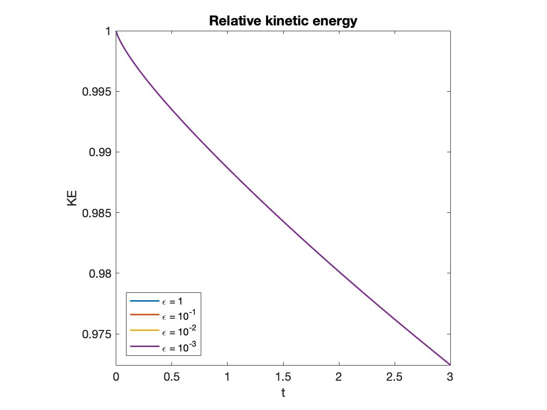
Figure 2. Relative kinetic energy from $t=0$ to $t=3.0$ for different values of $\varepsilon$.

6.3. Asymptotic Consistency

This test problem is to demonstrate the AP property. Let us consider the following well-prepared initial data similar to that in [11].

(6.4) $$\rho(0,x_{1},x_{2}) =1+\varepsilon^{2}\sin^{2}(2\pi(x_{1}+x_{2})),$$

$$u(0,x_{1},x_{2}) =\sin(2\pi(x_{1}-x_{2}))+\varepsilon\sin(2\pi(x_{1}+x_{2})),$$

$$u(0,x_{1},x_{2}) =\sin(2\pi(x_{1}-x_{2}))+\varepsilon\cos(2\pi(x_{1}+x_{2})).$$

We set a very small value of $\varepsilon$, namely $\varepsilon=10^{-4}$. The computational domain $[0,1]\times[0,1]$ is divided into an under resolved mesh of $40\times 40$ cells. The boundaries are all taken to be periodic, and the CFL is 0.45. The linearisation parameters are $(\underline{u}_{1},\underline{u}_{2})=(1,1)$ , $\underline{\rho}=1$ and $\underline{a}=1$. The final time is $T=3$.

In Figure 3 we plot the density and the divergence of the velocity at time $T=0$. Note that the density perturbation is $O(\varepsilon^{2})$ and the divergence perturbation is $O(\varepsilon)$ initially. The corresponding plots obtained using the numerical solution at time $T=3$, clearly show that the density is almost constant, and the velocity divergence is zero. Hence, we culminate that the numerical solution approximates the incompressible solution $\rho_{(0)}=\mathrm{const.}$, and $\nabla\cdot u_{(0)}=0$, demonstrating the AP property of the scheme. Further, we show in Figure 4 the transient behaviour of $\lVert\nabla\rho\rVert_{L_{2}}$ and $\lVert\nabla\cdot u\rVert_{L_{2}}$ verses time, from $t=0$ to $t=3$. The figure clearly shows that if the initial data is close to an incompressible data, then the numerical solution remains close to $\mathcal{E}$ for all times.

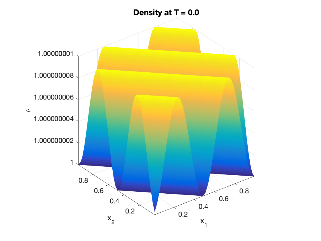
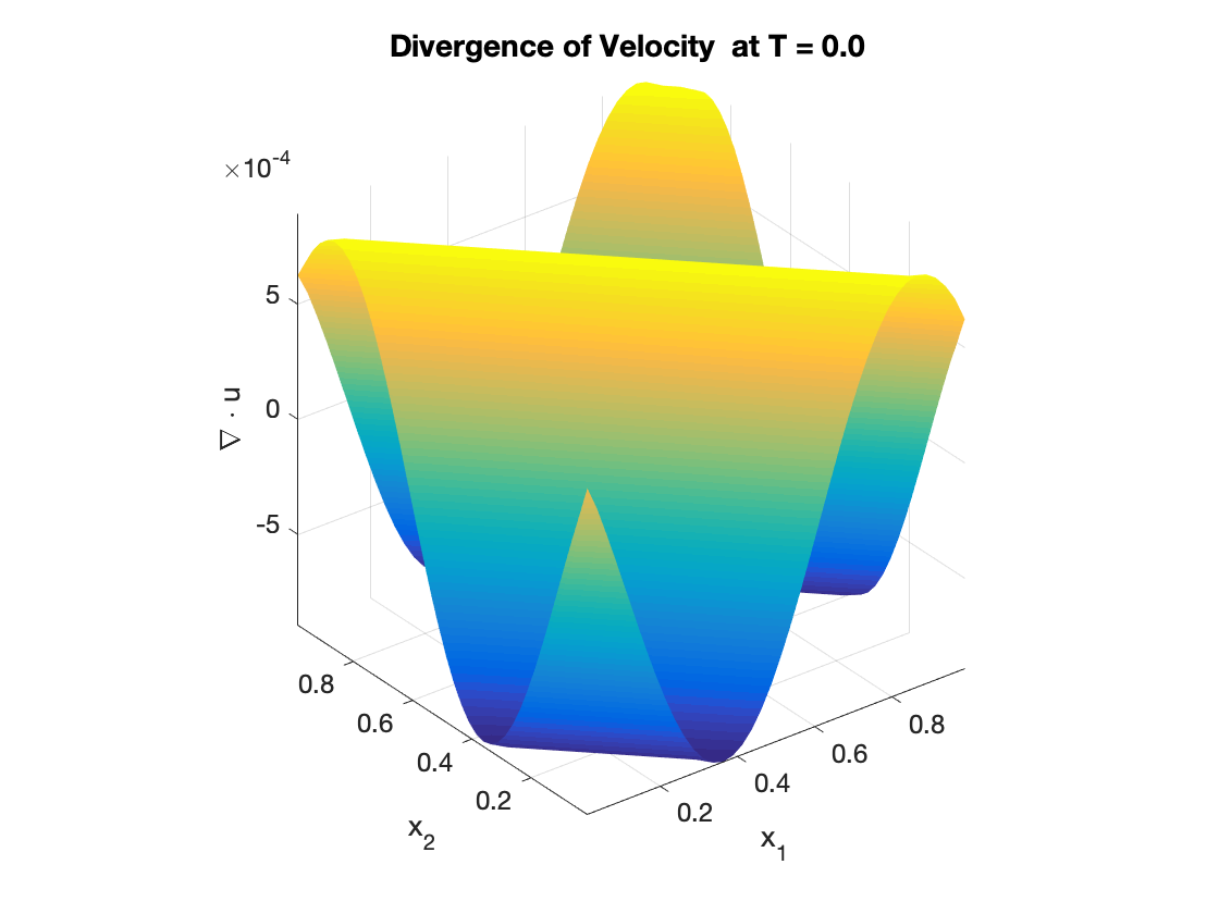
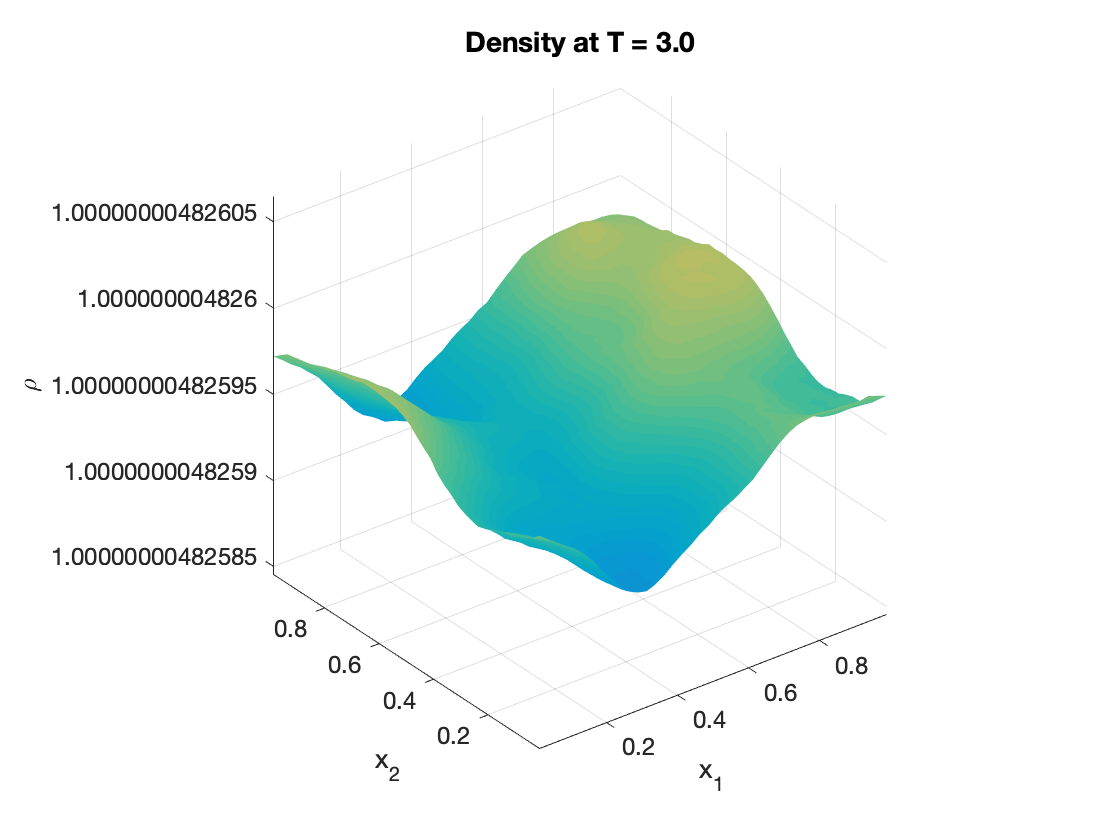
Figure 3. Top Left: $\rho$ at $T=0.0$ . Top Right: $\nabla\cdot u$ at $T=0.0$. Bottom Left: $\rho$ at $T=3.0$. Bottom right: $\nabla\cdot u$ at $T=3.0$. Here, $\varepsilon=10^{-4}$.

Figure 4. Left: $\lVert\nabla\rho\rVert_{L^{2}}$ from time $T=0$ to 3. Right: $\lVert\nabla\cdot u\rVert_{L^{2}}$ from time $T=0$ to 3. Here, $\varepsilon=10^{-4}$.

6.4. Asymptotic Order of Convergence and $\mathcal{E}$-invariance

The aim of this experiment is to numerically validate the second order asymptotic convergence of the numerical solution to the incompressible limit solution. To this end, we consider the following exact solution of the incompressible system (1.4) considered in [25], in which $\varrho_{(0)}(t,x_{1},x_{2})=1$, and

(6.5) $$u_{1,(0)}(t,x_{1},x_{2}) =1-2\cos(2\pi(x_{1}-t))\sin(2\pi(x_{2}-t)),$$

$$u_{2,(0)}(t,x_{1},x_{2}) =1+2\sin(2\pi(x_{1}-t))\cos(2\pi(x_{2}-t)),$$

$$\varrho_{(1)}(t,x_{1},x_{2}) =-\cos(4\pi(x_{1}-t))-\cos(4\pi(x_{2}-t)).$$

The linearisation parameters are $\underline{\rho}=1,\underline{a}=1$ and $(\underline{u}_{1},\underline{u}_{2})=(1,1)$. The computational domain $\Omega=[0,1]\times[0,1]$ is successively divided into $20\times 20$, $40\times 40$, $80\times 80$, and $160\times 160$ mesh cells and the CFL number used is 0.45. The initial data used is obtained by setting $\varrho(0,x_{1},x_{2})=\varrho_{(0)}(0,x_{1},x_{2}),u_{1}(0,x_{1},x_{2})=u_{1,(0)}(0,x_{1},x_{2})$ and $u_{2}(0,x_{1},x_{2})=u_{2,(0)}(0,x_{1},x_{2})$. The boundaries are assumed to be periodic in nature and the final time for computation is $T=3.0$.

First, the plot of the $l^{1}$-norm of the gradient of the density and the divergence of the velocity at the initial time, and at final time $T=3$ is given in Figure 5, with an under-resolved $40\times 40$ mesh for $\varepsilon=10^{-4}$. The Figure clearly shows that the IMEX-RK scheme leaves the well-prepared space invariant as the density is a constant, and the velocity is divergence-free.

As defined in [2], the EOC computed using incompressible data $(\varrho_{(0)},u_{1,(0)},u_{2,(0)})$, as the reference solution is termed as the asymptotic order of convergence (AOC).The numerical results obtained show that the density $\varrho$ remains constant exactly at $1$, and hence both the velocity components are used to measure the AOC. We compute the AOC for very small values of $\varepsilon$, namely for $\varepsilon=10^{-3}$ and $\varepsilon=10^{-4}$. The AOC obtained in both the $L^{1}$ and $L^{2}$ norms are presented in Tables 5 and 6. From the tables it can easily be seen that as $\varepsilon\to 0$ the numerical solution converges to the incompressible solution with second order accuracy. This observation reiterate also the fact that the chosen variant ARS(2,2,2) is stiffly accurate; see also [3].

In Figure 6 we plot the $L^{2}$ norms of the gradient of the density and divergence of the velocity over the entire computational time range $T\in[0,3]$. It clearly shows that the numerical solution stays in $\mathcal{E}$ for all times. Hence, it substantiate the $\mathcal{E}$-invariance with respect to time

$N$	$L^{1}$ error in $u_{1}$	AOC	$L^{2}$ error in $u_{1}$	AOC	$L^{1}$error in $u_{2}$	AOC	$L^{2}$ error in $u_{2}$	AOC
20	2.670e-01		3.034e-01		2.670e-01		3.034e-01
40	6.931e-02	1.9461	7.749e-02	1.9692	6.931e-02	1.9461	7.749e-02	1.9692
80	1.734e-02	1.9984	1.930e-02	2.0054	1.734e-02	1.9984	1.930e-02	2.0054
160	4.332e-03	2.0015	4.814e-03	2.0034	4.332e-03	2.0015	4.814e-03	2.0034

Table 5. $L^{1}$, $L^{2}$ errors in $u_{1}$, $u_{2}$, and AOC for Problem 6.4 corresponding to $\varepsilon=10^{-3}$.

$N$	$L^{1}$ error in $u_{1}$	AOC	$L^{2}$ error in $u_{1}$	AOC	$L^{1}$error in $u_{2}$	AOC	$L^{2}$ error in $u_{2}$	AOC
20	2.670e-01		3.034e-01		2.670e-01		3.034e-01
40	6.931e-02	1.9461	7.749e-02	1.9692	6.931e-02	1.9461	7.749e-02	1.9692
80	1.734e-02	1.9984	1.930e-02	2.0054	1.734e-02	1.9984	1.930e-02	2.0054
160	4.332e-03	2.0015	4.814e-03	2.0034	4.332e-03	2.0015	4.814e-03	2.0034

Table 6. $L^{1}$, $L^{2}$ errors in $u_{1}$, $u_{2}$, and AOC for Problem 6.4 corresponding to $\varepsilon=10^{-4}$.

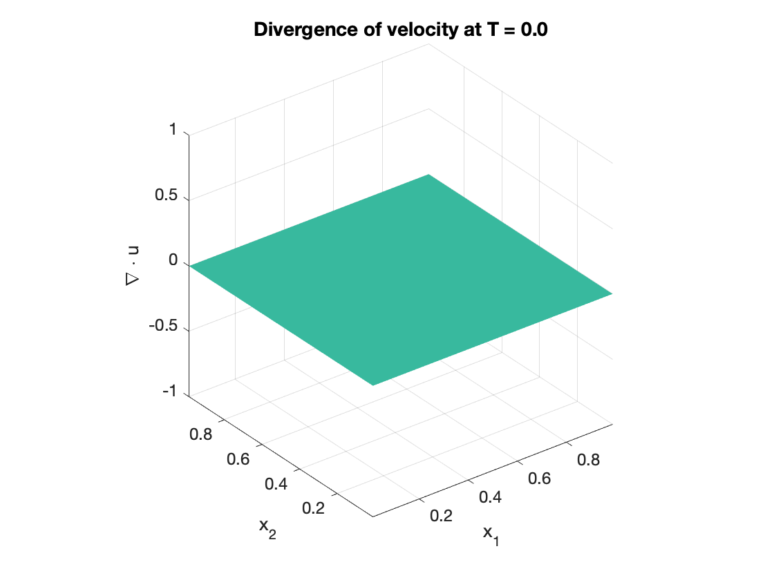
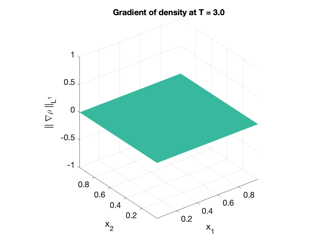
Figure 5. Top Left: $\lVert\nabla\rho\rVert_{l^{1}}$ at $T=0$. Top Right: $\nabla\cdot u$ at $T=0$. Bottom Left: $\lVert\nabla\rho\rVert_{l^{1}}$ at $T=3$. Bottom right: $\nabla\cdot u$ at $T=3$. Here, $\varepsilon=10^{-4}$.

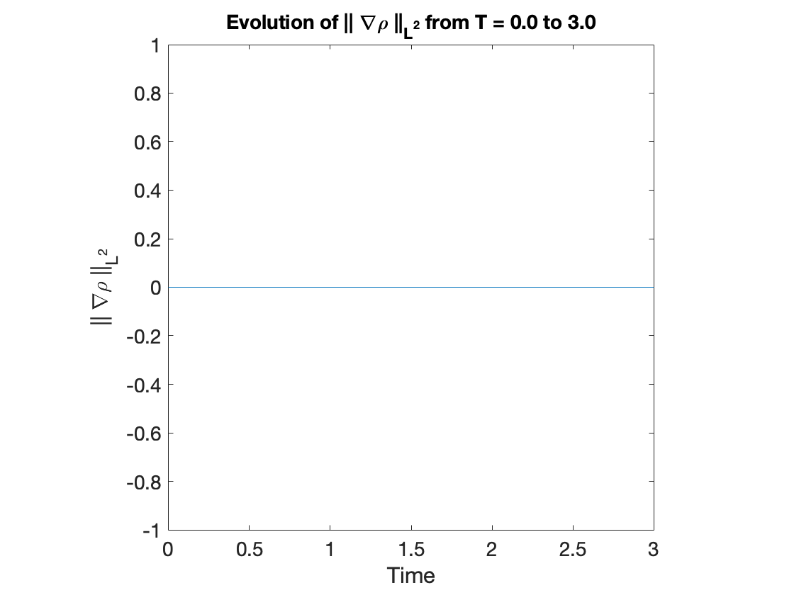
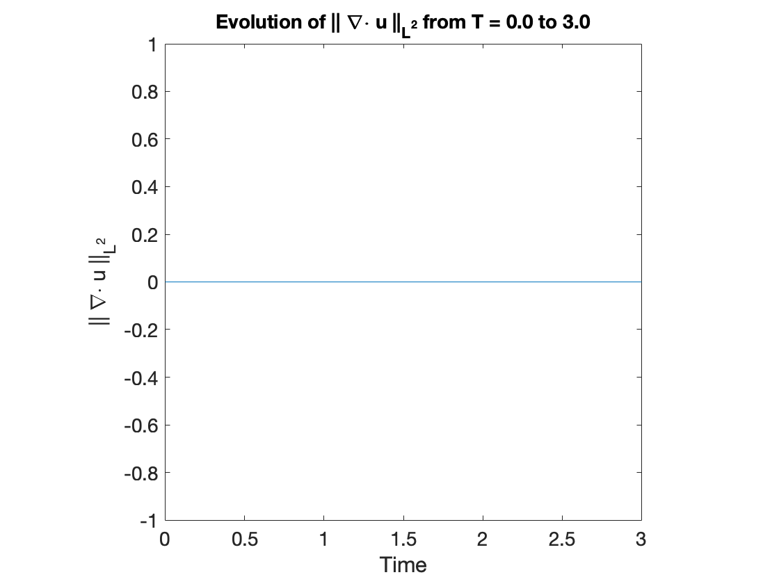
Figure 6. Left: $\lVert\nabla\rho\rVert_{L^{2}}$ from time $T=0$ to 3. Right: $\lVert\nabla\cdot u\rVert_{L^{2}}$ from time $T=0$ to 3. Here, $\varepsilon=10^{-4}$.

7. Concluding Remarks

In this paper, we have presented a detailed analysis of an IMEX-RK finite volume scheme for the linear wave equation system in the zero Mach number regime. The existence of a unique numerical solution, its uniform stability with respect to $\varepsilon$, the AP property, and the asymptotic accuracy are shown for the time semi-discrete scheme using saddle point theory of variational problems. Results from the theory of circulant matrices are used to establish the same features for the space-time fully-discrete scheme, obtained via a finite volume discretisation. Extensive numerical studies are carried out to test the various theoretical concepts discussed. Uniform second-order convergence is achieved with respect to $\varepsilon$, experimentally. The dissipation of the scheme is shown to be independent of $\varepsilon$. The experiments reveal that the scheme is AP, and also achieves second-order asymptotic convergence, leaving the well-prepared space $\mathcal{E}$ invariant. Hence, the numerical case studies validate all the theoretical findings.

References

- [1] K. R. Arun, A. J. Das Gupta, and S. Samantaray. An implicit-explicit scheme accurate at low Mach numbers for the wave equation system. In Theory, numerics and applications of hyperbolic problems. I, volume 236 of Springer Proc. Math. Stat., pages 97–109. Springer, Cham, 2018.
- [2] K. R. Arun and S. Samantaray. Asymptotic Preserving and Low Mach Number Accurate IMEX Finite Volume Schemes for the Euler Equations. arXiv e-prints, page arXiv:1907.01711, Jul 2019.
- [3] U. M. Ascher, S. J. Ruuth, and R. J. Spiteri. Implicit-explicit Runge-Kutta methods for time-dependent partial differential equations. Appl. Numer. Math., 25(2-3):151–167, 1997. Special issue on time integration (Amsterdam, 1996).
- [4] D. S. Bernstein. Matrix mathematics. Princeton University Press, Princeton, NJ, second edition, 2009. Theory, facts, and formulas.
- [5] G. Bispen, K. R. Arun, M. Lukáčová-Medvid’ová, and S. Noelle. IMEX large time step finite volume methods for low Froude number shallow water flows. Commun. Comput. Phys., 16(2):307–347, 2014.
- [6] F. Brezzi and M. Fortin. Mixed and hybrid finite element methods, volume 15 of Springer Series in Computational Mathematics. Springer-Verlag, New York, 1991.
- [7] P. G. Ciarlet. Linear and Nonlinear Functional Analysis with Applications. Society for Industrial and Applied Mathematics, Philadelphia, PA, USA, 2013.
- [8] F. Cordier, P. Degond, and A. Kumbaro. An asymptotic-preserving all-speed scheme for the Euler and Navier-Stokes equations. J. Comput. Phys., 231(17):5685–5704, 2012.
- [9] P. Degond. Asymptotic-preserving schemes for fluid models of plasmas. In Numerical models for fusion, volume 39/40 of Panor. Synthèses, pages 1–90. Soc. Math. France, Paris, 2013.
- [10] P. Degond, F. Deluzet, A. Lozinski, J. Narski, and C. Negulescu. Duality-based asymptotic-preserving method for highly anisotropic diffusion equations. Commun. Math. Sci., 10(1):1–31, 2012.
- [11] P. Degond and M. Tang. All speed scheme for the low Mach number limit of the isentropic Euler equations. Commun. Comput. Phys., 10(1):1–31, 2011.
- [12] S. Dellacherie. Analysis of Godunov type schemes applied to the compressible Euler system at low Mach number. J. Comput. Phys., 229(4):978–1016, 2010.
- [13] R. M. Gray. Toeplitz and circulant matrices:, 2006. A review.
- [14] E. Hairer and G. Wanner. Solving ordinary differential equations. II, volume 14 of Springer Series in Computational Mathematics. Springer-Verlag, Berlin, second edition, 1996. Stiff and differential-algebraic problems.
- [15] R. A. Horn and C. R. Johnson. Matrix analysis. Cambridge University Press, Cambridge, 1985.
- [16] R. A. Horn and C. R. Johnson. Topics in matrix analysis. Cambridge University Press, Cambridge, 1991.
- [17] S. Jin. Efficient asymptotic-preserving (AP) schemes for some multiscale kinetic equations. SIAM J. Sci. Comput., 21(2):441–454, 1999.
- [18] S. Jin. Asymptotic preserving (AP) schemes for multiscale kinetic and hyperbolic equations: a review. Riv. Math. Univ. Parma (N.S.), 3(2):177–216, 2012.
- [19] C. A. Kennedy and M. H. Carpenter. Additive Runge-Kutta schemes for convection-diffusion-reaction equations. Applied Numerical Mathematics, 44(1):139 – 181, 2003.
- [20] S. Klainerman and A. Majda. Singular limits of quasilinear hyperbolic systems with large parameters and the incompressible limit of compressible fluids. Comm. Pure Appl. Math., 34(4):481–524, 1981.
- [21] R. Klein. Semi-implicit extension of a Godunov-type scheme based on low Mach number asymptotics. I. One-dimensional flow. J. Comput. Phys., 121(2):213–237, 1995.
- [22] S. Noelle, G. Bispen, K. R. Arun, M. Lukáčová-Medviďová, and C.-D. Munz. A weakly asymptotic preserving low Mach number scheme for the Euler equations of gas dynamics. SIAM J. Sci. Comput., 36(6):B989–B1024, 2014.
- [23] L. Pareschi and G. Russo. Implicit-explicit Runge-Kutta schemes for stiff systems of differential equations. In Recent trends in numerical analysis, volume 3 of Adv. Theory Comput. Math., pages 269–288. Nova Sci. Publ., Huntington, NY, 2001.
- [24] L. Pareschi and G. Russo. Implicit-Explicit Runge-Kutta schemes and applications to hyperbolic systems with relaxation. J. Sci. Comput., 25(1-2):129–155, 2005.
- [25] T. Schneider, N. Botta, K. J. Geratz, and R. Klein. Extension of finite volume compressible flow solvers to multi-dimensional, variable density zero Mach number flows. J. Comput. Phys., 155(2):248–286, 1999.
- [26] H. Zakerzadeh. Asymptotic Preserving Finite Volume Schemes For The Singularly-perturbed Shallow Water Equations with Source Terms. PhD thesis, RWTH Aachen, Germany, 2017.
- [27] H. Zakerzadeh and S. Noelle. A note on the stability of implicit-explicit flux-splittings for stiff systems of hyperbolic conservation laws. Commun. Math. Sci., 16(1):1–15, 2018.