Refined dimensional reduction for isotropic elastic Cosserat shells with initial curvature

Abstract

Using a geometrically motivated 8-parameter ansatz through the thickness, we reduce a three-dimensional shell-like geometrically nonlinear Cosserat material to a fully two-dimensional shell model. Curvature effects are fully taken into account. For elastic isotropic Cosserat materials, the integration through the thickness can be performed analytically and a generalized plane stress condition allows for a closed-form expression of the thickness stretch and the nonsymmetric shift of the midsurface in bending. We obtain an explicit form of the elastic strain energy density for Cosserat shells, including terms up to order $O(h^{5})$ in the shell thickness $h$. This energy density is expressed as a quadratic function of the nonlinear elastic shell strain tensor and the bending-curvature tensor, with coefficients depending on the initial curvature of the shell.

Dedicated to Sanda Cleja-Ţigoiu on the occasion of her 70th birthday

1 Introduction

Nonlinear elastic shell theory is a notoriously difficult subject from the perspective of modelling, analysis and numerical implementation. Some successful research has been devoted to generalizations of the Reissner-Mindlin kinematics, well known from linear elastic plate models [22]. In his habilitation thesis, the last author of the present article began the modelling and analysis of so-called nonlinear Cosserat shell models, in which a full triad of orthogonal directors, independent of the normal of the shell, is taken into account [16, 15, 19, 21]. As such, these models fall into the class of 6-parameter shell models, proposed originally by Reissner [28] and presented in the book of Libai and Simmonds [14] as well as in the works of Pietraszkiewicz and coauthors [12, 10, 13], see also [36, 35]. They are also the preferred models from an engineering point of view, since the independent rotation field allows for transparent coupling between shell and beam parts.

The results of [16, 15, 19] have been obtained by an 8-parameter ansatz of the deformation through the thickness and consistent analytic integration over the thickness in the case of a flat undeformed shell reference configuration. The mathematical approach developed there also allowed for the first existence proof of minimizers [15, 19, 1]. In this paper, we extend the modelling from flat shells to initially curved shells. With appropriate changes, taking into account the geometry of the shell, it is possible to use the same derivation ideas. Our ansatz allows for a consistent shell model up to order $O(h^{5})$ in the shell thickness. Interestingly, the contributions of order $h^{5}$ in the shell energy all depend on the initial curvature of the shell and vanish for a flat-shell. In this case we recover the previously mentioned flat Cosserat shell model [15]. The $h^{5}$-contribution does not come with a definite sign, such that the additional terms can be stabilizing as well as destabilizing, depending on the local shell geometry.

However, all occurring material coefficients of the shell model are uniquely determined from the isotropic three-dimensional Cosserat model and the given initial geometry of the shell. Thus, we fill a certain gap in the general 6-parameter shell theory, which leaves the precise structure of the constitutive equations wide open.

In a future contribution we will try to prove the existence of minimizers for our new Cosserat shell model along the methods outlined in [1].

2 The three-dimensional Cosserat model in curvilinear coordinates

Let $\Omega_{\xi}\subset\mathbb{R}^{3}$ be the reference configuration of an elastic Cosserat body. The elastic material occupying the domain $\Omega_{\xi}$ is assumed to be homogeneous and isotropic. A generic point of $\Omega_{\xi}$ will be denoted by $(\xi_{1},\xi_{2},\xi_{3})$. The deformation of the body is described by a vectorial map $\boldsymbol{\varphi}_{\xi}$ (called deformation) and a microrotation tensor $\boldsymbol{R}_{\xi}$:

$$\boldsymbol{\varphi}_{\xi}:\Omega_{\xi}\rightarrow\mathbb{R}^{3},\qquad\boldsymbol{R}_{\xi}:\Omega_{\xi}\rightarrow\mathrm{SO}(3)\,.$$ (2.1)

We denote by $\Omega_{c}:=\boldsymbol{\varphi}_{\xi}(\Omega_{\xi})$ the current (deformed) configuration.

Throughout the paper, we adhere to some common notational conventions: boldface letters denote vectors and tensors; the Latin indices $i,j,k,...$ range over the set $\{1,2,3\}$, while the Greek indices $\alpha,\beta,\gamma,...$ take the values $\{1,2\}$. We also employ the Einstein summation convention over repeated indices.

Consider a parametric representation

$$\boldsymbol{\Theta}:\Omega_{h}\rightarrow\Omega_{\xi}\,,\qquad\boldsymbol{\Theta}(x_{1},x_{2},x_{3})=(\xi_{1},\xi_{2},\xi_{3})=\xi_{i}\boldsymbol{e}_{i}\,,$$ (2.2)

of the domain $\Omega_{\xi}$, where $\boldsymbol{\Theta}$ is a $C^{1}$-diffeomorphism and $\Omega_{h}\subset\mathbb{R}^{3}$ is the parameter domain. Here, the domains $\Omega_{h}$ and $\Omega_{\xi}$ are equipped with a right Cartesian coordinate frame with unit vectors $\boldsymbol{e}_{i}$ along the axes $Ox_{i}\,$, see Figure 1. Thus, the domain $\Omega_{h}$ can be viewed as a “fictitious flat Cartesian configuration” of the body. In view of (2.2), we can regard $(x_{1},x_{2},x_{3})$ as curvilinear coordinates on $\Omega_{\xi}\,$. The special form of the parameter domain $\Omega_{h}$ and of the parametrization function $\boldsymbol{\Theta}$ appropriate to thin shells will be introduced in the next section.

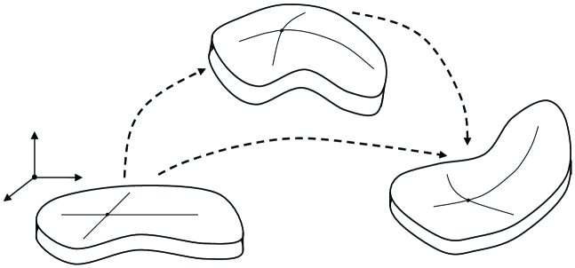
Figure 1: The reference configuration $\Omega_{\xi}$ of the shell, the current configuration $\Omega_{c}$ and the “fictitious flat Cartesian configuration” $\Omega_{h}\,$.

With respect to these curvilinear coordinates $x_{i}$ $(i=1,2,3)$, we use the covariant base vectors $\boldsymbol{g}_{i}$ and the contravariant base vectors $\boldsymbol{g}^{i}$ given by

$$\boldsymbol{g}_{i}=\dfrac{\partial\boldsymbol{\Theta}}{\partial x_{i}}\,=\dfrac{\partial\xi_{j}}{\partial x_{i}}\,\boldsymbol{e}_{j}\,,\qquad\boldsymbol{g}^{i}=\nabla_{\xi}\,x_{i}\,=\dfrac{\partial x_{i}}{\partial\xi_{j}}\,\boldsymbol{e}_{j}\,,\qquad\boldsymbol{g}^{j}\cdot\boldsymbol{g}_{i}=\delta^{j}_{i}\,,$$ (2.3)

where we denote by $\cdot$ the scalar product and $\delta^{j}_{i}$ is the Kronecker symbol. Using the parametrization $\boldsymbol{\Theta}$, the deformation function $\boldsymbol{\varphi}$ may be written as the composition

$$\boldsymbol{\varphi}:=\boldsymbol{\varphi}_{\xi}\circ\boldsymbol{\Theta}:\Omega_{h}\rightarrow\Omega_{c}\,,\qquad\boldsymbol{\varphi}(x_{1},x_{2},x_{3}):=\boldsymbol{\varphi}_{\xi}\big{(}\boldsymbol{\Theta}(x_{1},x_{2},x_{3})\big{)}.$$ (2.4)

The gradient of $\boldsymbol{\Theta}$ can be represented as

$$\nabla_{x}\boldsymbol{\Theta}=\dfrac{\partial\boldsymbol{\Theta}}{\partial x_{i}}\,\,\otimes\boldsymbol{e}_{i}=\boldsymbol{g}_{i}\otimes\boldsymbol{e}_{i}\qquad\textrm{and}\qquad\big{(}\nabla_{x}\boldsymbol{\Theta}\big{)}^{-1}=\boldsymbol{e}_{i}\otimes\boldsymbol{g}^{i},$$ (2.5)

where $\otimes$ denotes the diadic product. The polar decomposition of $\nabla_{x}\boldsymbol{\Theta}$ is denoted by

$$\nabla_{x}\boldsymbol{\Theta}={\boldsymbol{Q}}_{0}\,\boldsymbol{U}_{0}=\operatorname{polar}{(\nabla_{x}\boldsymbol{\Theta})}\,{\boldsymbol{U}}_{0}\,,$$ (2.6)

where $\,{\boldsymbol{Q}}_{0}=\operatorname{polar}{(\nabla_{x}\boldsymbol{\Theta})}\in\rm{SO}(3)$ is a pure rotation and $\,{\boldsymbol{U}}_{0}\,$ is a positive definite symmetric tensor [24]. Based on the polar factor ${\boldsymbol{Q}}_{0}$, we define the orthonormal directors $\boldsymbol{d}_{1}^{0}\,,\,\boldsymbol{d}_{2}^{0}\,,\,\boldsymbol{d}_{3}^{0}$ in the reference configuration $\Omega_{\xi}$ by

$$\boldsymbol{d}_{i}^{0}:=\boldsymbol{Q}_{0}\,\boldsymbol{e}_{i}\,,\qquad\mbox{i.e.}\qquad\boldsymbol{Q}_{0}=\boldsymbol{d}_{i}^{0}\otimes\boldsymbol{e}_{i}\,.$$ (2.7)

Furthermore, we introduce the elastic microrotation $\boldsymbol{Q}_{e}$ as the composition

$$\boldsymbol{Q}_{e}=\boldsymbol{R}_{\xi}\circ\boldsymbol{\Theta}:\Omega_{h}\rightarrow\mathrm{SO}(3),\qquad\boldsymbol{Q}_{e}(\boldsymbol{x}):=\boldsymbol{R}_{\xi}\big{(}\boldsymbol{\Theta}(\boldsymbol{x})\big{)},$$ (2.8)

where $\boldsymbol{x}:=(x_{1},x_{2},x_{3})=x_{i}\boldsymbol{e}_{i}\,$. Then the orthonormal directors $\boldsymbol{d}_{1}\,,\,\boldsymbol{d}_{2}\,,\,\boldsymbol{d}_{3}$ in the current configuration $\Omega_{c}$ are given by

$$\boldsymbol{d}_{i}:=\boldsymbol{Q}_{e}\boldsymbol{d}^{0}_{i}\,,\qquad\mbox{i.e.}\qquad\boldsymbol{Q}_{e}=\boldsymbol{d}_{i}\otimes\boldsymbol{d}_{i}^{0}\,;$$ (2.9)

these directors describe the orientation of the material points of the Cosserat medium and characterize the microrotation field. Moreover, the total microrotation $\overline{\boldsymbol{R}}$ is given by

$$\overline{\boldsymbol{R}}:\Omega_{h}\rightarrow\mathrm{SO}(3),\qquad\overline{\boldsymbol{R}}(\boldsymbol{x}):=\boldsymbol{Q}_{e}(\boldsymbol{x})\,\boldsymbol{Q}_{0}(\boldsymbol{x})\,.$$ (2.10)

In particular,

$$\overline{\boldsymbol{R}}(\boldsymbol{x})=(\boldsymbol{d}_{i}\otimes\boldsymbol{d}_{i}^{0})\,(\boldsymbol{d}_{j}^{0}\otimes\boldsymbol{e}_{j})=\boldsymbol{d}_{i}(\boldsymbol{x})\otimes\boldsymbol{e}_{i}\,.$$ (2.11)

Remark: We write the microrotation tensor $\overline{\boldsymbol{R}}$ with a superposed bar in order to distinguish it from the orthogonal factor ${\boldsymbol{R}}$ in the classical polar decomposition of the deformation gradient $\boldsymbol{F}=\boldsymbol{R}\,\boldsymbol{U}\,$, which is a common notational convention in nonlinear elasticity. $\Box$

The deformation gradient corresponding to the deformation $\boldsymbol{\varphi}_{\xi}$ is given by

$$\boldsymbol{F}_{\xi}:=\nabla_{\xi}\,\boldsymbol{\varphi}_{\xi}=\dfrac{\partial\boldsymbol{\varphi}_{\xi}}{\partial\xi_{i}}\,\,\otimes\boldsymbol{e}_{i}\,,$$ (2.12)

whereas $\boldsymbol{F}$ denotes the gradient of the deformation function $\boldsymbol{\varphi}$ with respect to $\boldsymbol{x}$, i.e.

$$\boldsymbol{F}:=\nabla_{x}\,\boldsymbol{\varphi}=\dfrac{\partial\boldsymbol{\varphi}}{\partial x_{i}}\,\,\otimes\boldsymbol{e}_{i}\,.$$ (2.13)

Thus

$$\boldsymbol{F}_{\xi}=\boldsymbol{F}\big{(}\nabla_{x}\boldsymbol{\Theta}\big{)}^{-1}$$ (2.14)

since, due to (2.3), (2.5) and the chain rule,

$$\boldsymbol{F}\,=\,\dfrac{\partial\boldsymbol{\varphi}_{\xi}}{\partial\xi_{j}}\,\dfrac{\partial\xi_{j}}{\partial x_{i}}\,\otimes\boldsymbol{e}_{i}\,=\,\dfrac{\partial\boldsymbol{\varphi}_{\xi}}{\partial\xi_{j}}\,(\boldsymbol{e}_{j}\cdot\boldsymbol{g}_{i})\,\otimes\boldsymbol{e}_{i}\,=\Big{(}\dfrac{\partial\boldsymbol{\varphi}_{\xi}}{\partial\xi_{j}}\otimes\boldsymbol{e}_{j}\Big{)}(\boldsymbol{g}_{i}\otimes\boldsymbol{e}_{i})=\boldsymbol{F}_{\xi}\big{(}\nabla_{x}\boldsymbol{\Theta}\big{)}.$$

By virtue of (2.5) and (2.13), the relation (2.14) can also be written as

$$\boldsymbol{F}_{\xi}=\Big{(}\dfrac{\partial\boldsymbol{\varphi}}{\partial x_{i}}\otimes\boldsymbol{e}_{i}\Big{)}(\boldsymbol{e}_{j}\otimes\boldsymbol{g}^{j})=\dfrac{\partial\boldsymbol{\varphi}}{\partial x_{i}}\,\,\otimes\boldsymbol{g}^{i}=\boldsymbol{\varphi},_{i}\otimes\,\boldsymbol{g}^{i}\,,$$ (2.15)

where an index $i$ preceded by a comma denotes partial differentiation with respect to $x_{i}$ .

For the non-symmetric Biot-type stretch tensor

$$\overline{\boldsymbol{U}}_{\xi}:=\boldsymbol{R}_{\xi}^{T}\,\boldsymbol{F}_{\xi}\qquad\textrm{and}\qquad\overline{\boldsymbol{U}}_{e}(\boldsymbol{x}):=\overline{\boldsymbol{U}}_{\xi}\big{(}\boldsymbol{\Theta}(\boldsymbol{x})\big{)}\,,$$ (2.16)

we find, using (2.8), (2.9) and (2.14),

$$\overline{\boldsymbol{U}}_{e}=\boldsymbol{Q}_{e}^{T}\,\boldsymbol{F}\big{(}\nabla_{x}\boldsymbol{\Theta}\big{)}^{-1}=\big{(}\boldsymbol{d}_{i}^{0}\otimes\boldsymbol{d}_{i}\big{)}\,\big{(}\boldsymbol{\varphi},_{j}\otimes\boldsymbol{g}^{j}\big{)}=\big{(}\boldsymbol{\varphi},_{j}\cdot\,\boldsymbol{d}_{i}\big{)}\,\big{(}\boldsymbol{d}_{i}^{0}\otimes\boldsymbol{g}^{j}\big{)}.$$ (2.17)

We denote by ${\boldsymbol{\mathbbm{1}}}_{3}=\boldsymbol{g}_{j}\otimes\boldsymbol{g}^{j}$ the three-dimensional unit tensor and introduce the non-symmetric strain tensor

$$\overline{\boldsymbol{E}}:=\overline{\boldsymbol{U}}_{e}-{\boldsymbol{\mathbbm{1}}}_{3}=\big{(}\boldsymbol{\varphi},_{j}\cdot\,\boldsymbol{d}_{i}-\boldsymbol{g}_{j}\cdot\boldsymbol{d}_{i}^{0}\big{)}\,\big{(}\boldsymbol{d}_{i}^{0}\otimes\boldsymbol{g}^{j}\big{)},$$ (2.18)

which is a Lagrangian strain measure for stretch [26]. As a Lagrangian strain measure for curvature (orientation change), we employ the so-called wryness tensor (see e.g., [23, 4])

$$\boldsymbol{\Gamma}_{\xi}:=\mathrm{axl}\big{(}\boldsymbol{R}_{\xi}^{T}\,\partial_{\xi_{i}}\boldsymbol{R}_{\xi}\big{)}\otimes\boldsymbol{e}_{i}\,,$$ (2.19)

where $\mathrm{axl}(\cdot)$ is the axial vector of any skew-symmetric tensor and $\partial_{\xi_{i}}$ denotes the partial differentiation with respect to $\xi_{i}\,$. In the following, we will show that

$$\boldsymbol{\Gamma}=\mathrm{axl}\big{(}\boldsymbol{Q}_{e}^{T}\boldsymbol{Q}_{e,k}\big{)}\otimes\boldsymbol{g}^{k}\,,\qquad\textrm{where}\qquad\boldsymbol{\Gamma}(\boldsymbol{x}):=\boldsymbol{\Gamma}_{\xi}\big{(}\boldsymbol{\Theta}(\boldsymbol{x})\big{)}.$$ (2.20)

In order to establish (2.20), we need to show that

$$\mathrm{axl}\big{(}\boldsymbol{Q}_{e}^{T}\boldsymbol{Q}_{e,k}\big{)}\otimes\boldsymbol{g}^{k}=\mathrm{axl}\big{(}\boldsymbol{R}_{\xi}^{T}\,\partial_{\xi_{i}}\boldsymbol{R}_{\xi}\big{)}\otimes\boldsymbol{e}_{i}\,.$$ (2.21)

First, using the chain rule, we find

$$\boldsymbol{Q}_{e,k}=\dfrac{\partial}{\partial x_{k}}\,\,\boldsymbol{R}_{\xi}\big{(}\boldsymbol{\Theta}(\boldsymbol{x})\big{)}=\dfrac{\partial\boldsymbol{R}_{\xi}}{\partial\xi_{i}}\,\,\dfrac{\partial\xi_{i}}{\partial x_{k}}\qquad\Longrightarrow\qquad\boldsymbol{Q}_{e}^{T}\boldsymbol{Q}_{e,k}=\big{(}\boldsymbol{R}_{\xi}^{T}\,\partial_{\xi_{i}}\boldsymbol{R}_{\xi}\big{)}\,\dfrac{\partial\xi_{i}}{\partial x_{k}}\;.$$ (2.22)

Since $\mathrm{axl}(\boldsymbol{A})=-\frac{1}{2}\,\boldsymbol{\varepsilon}:\boldsymbol{A}$ for any skew-symmetric tensor $\boldsymbol{A}$, where $\boldsymbol{\varepsilon}$ is the alternating Ricci third-order tensor (see e.g. [3, 4]), relation (2.22) yields

$$\mathrm{axl}\big{(}\boldsymbol{Q}_{e}^{T}\boldsymbol{Q}_{e,k}\big{)}=\mathrm{axl}\big{(}\boldsymbol{R}_{\xi}^{T}\,\partial_{\xi_{i}}\boldsymbol{R}_{\xi}\big{)}\,\dfrac{\partial\xi_{i}}{\partial x_{k}}\;.$$ (2.23)

Therefore, since $\,\dfrac{\partial\xi_{i}}{\partial x_{k}}\,=\boldsymbol{e}_{i}\cdot\boldsymbol{g}_{k}\;$, equation (2.21) and thus (2.20) holds.

Using the relation $\,\boldsymbol{Q}_{e}=\overline{\boldsymbol{R}}\,\boldsymbol{Q}_{0}^{T}\,$ and the identity

$$\boldsymbol{Q}\,\mathrm{axl}(\boldsymbol{A})=\mathrm{axl}\big{(}\boldsymbol{Q}\boldsymbol{A}\boldsymbol{Q}^{T}\big{)}\,,$$

which is valid for any skew-symmetric tensor $\boldsymbol{A}\in\mathfrak{so}(3)$ and any $\boldsymbol{Q}\in\mathrm{SO}(3)$, we can write the relation (2.20) in the alternative form

$$\boldsymbol{\Gamma}=\boldsymbol{Q}_{0}\big{[}\mathrm{axl}\big{(}\overline{\boldsymbol{R}}^{T}\overline{\boldsymbol{R}}_{,i}\big{)}-\mathrm{axl}\big{(}\boldsymbol{Q}_{0}^{T}\boldsymbol{Q}_{0,i}\big{)}\big{]}\otimes\boldsymbol{g}^{i}\,.$$ (2.24)

The wryness tensor defined in (2.20) can also be written in the form

$$\boldsymbol{\Gamma}=\boldsymbol{\Gamma}_{e}\big{(}\nabla_{x}\boldsymbol{\Theta}\big{)}^{-1}\,,\qquad\textrm{where}\qquad\boldsymbol{\Gamma}_{e}:=\mathrm{axl}\big{(}\boldsymbol{Q}_{e}^{T}\boldsymbol{Q}_{e,i}\big{)}\otimes\boldsymbol{e}_{i}\;.$$ (2.25)

For a detailed discussion on various strain measures of non-linear micropolar continua we refer to the papers [26, 3].

We now turn to the constitutive relations. We assume that the elastically stored energy density $W(\overline{\boldsymbol{E}},\boldsymbol{\Gamma})$ admits the additive split

$$W(\overline{\boldsymbol{E}},\boldsymbol{\Gamma})=W_{\mathrm{mp}}(\overline{\boldsymbol{E}})+W_{\mathrm{curv}}(\boldsymbol{\Gamma})$$ (2.26)

into the elastic stretch (membrane) part $W_{\mathrm{mp}}$ and the curvature part $W_{\mathrm{curv}}$. For the elastic stretch part, we assume the form

$$\begin{array}[]{rcl}W_{\mathrm{mp}}(\overline{\boldsymbol{E}})&=&\mu\,\|\,\mathrm{sym}\,\overline{\boldsymbol{E}}\,\|^{2}\,+\,\mu_{c}\,\|\,\mathrm{skew}\,\overline{\boldsymbol{E}}\,\|^{2}\,+\,\dfrac{\lambda}{2}\,\big{(}\mathrm{tr}\,\overline{\boldsymbol{E}}\,\big{)}^{2}\vspace{4pt}\\ &=&\mu\,\|\,\mathrm{dev_{3}\,sym}\,\overline{\boldsymbol{E}}\,\|^{2}\,+\,\mu_{c}\,\|\,\mathrm{skew}\,\overline{\boldsymbol{E}}\,\|^{2}\,+\,\dfrac{\kappa}{2}\,\big{(}\mathrm{tr}\,\overline{\boldsymbol{E}}\,\big{)}^{2}\,,\end{array}$$ (2.27)

where $\lambda,\mu$ are the Lamé constants and $\kappa=\frac{3\lambda+2\mu}{3}\,$ is the bulk modulus of classical isotropic elasticity, while $\,\mu_{c}\geq 0$ is called the Cosserat couple modulus [17, 19]; here, we also employ the well-known operators

$$\mathrm{sym}\,\boldsymbol{X}=\frac{1}{2}\,(\boldsymbol{X}+\boldsymbol{X}^{T}),\qquad\mathrm{skew}\,\boldsymbol{X}=\frac{1}{2}\,(\boldsymbol{X}-\boldsymbol{X}^{T}),\qquad\,\mathrm{dev_{3}\,}\boldsymbol{X}=\boldsymbol{X}-\frac{1}{3}(\mathrm{tr}\,\boldsymbol{X})\,{\boldsymbol{\mathbbm{1}}}_{3}\,,$$ (2.28)

which represent the symmetric part, the skew-symmetric part and the deviatoric part, respectively, of any three-dimensional tensor $\boldsymbol{X}\,$. We also assume the standard restrictions

$$\mu>0,\qquad\kappa>0\quad\mathrm{and}\quad\mu_{c}\geq 0$$ (2.29)

on the constitutive coefficients.

For the curvature part $W_{\mathrm{curv}}(\boldsymbol{\Gamma})$ of the energy density, we use the form [20]

$$W_{\mathrm{curv}}(\boldsymbol{\Gamma})=\mu\,L_{c}^{2}\,\Big{(}\,b_{1}\,\|\,\mathrm{dev_{3}\,sym}\,\boldsymbol{\Gamma}\|^{2}\,+\,b_{2}\,\|\,\mathrm{skew}\,\boldsymbol{\Gamma}\|^{2}\,+\,b_{3}\big{(}\mathrm{tr}\,\boldsymbol{\Gamma}\big{)}^{2}\,\Big{)}\,,$$ (2.30)

where $b_{1}\,,\,b_{2}\,,\,b_{3}>0$ are dimensionless constitutive coefficients and the parameter $\,L_{c}>0\,$ introduces an internal length which is characteristic for the material and is responsible for size effects of the Cosserat model. We notice that the energy density (2.26) is a quadratic function, which corresponds to a physically linear response.

Assuming that no external body and surface forces and no external volume or surface couples are present, the deformation and the microrotation solve the geometrically nonlinear minimization problem

$$I=\displaystyle\int_{\Omega_{\xi}}\widetilde{W}\big{(}\boldsymbol{F}_{\xi},{\boldsymbol{R}}_{\xi}\,\big{)}\,\mathrm{d}V\quad\to\quad\textrm{\ \ min\ \ w.r.t.\ \ }(\boldsymbol{\varphi}_{\xi},{\boldsymbol{R}}_{\xi}\,)\,,$$ (2.31)

posed on $\Omega_{\xi}\,$, where $\widetilde{W}\big{(}\boldsymbol{F}_{\xi},{\boldsymbol{R}}_{\xi}\,\big{)}=W(\overline{\boldsymbol{E}},\boldsymbol{\Gamma})$ is the energy density. Making the change of variables $(\xi_{1},\xi_{2},\xi_{3})=\boldsymbol{\Theta}(\boldsymbol{x})$ in the above integral we can write the total energy functional $I$ as the integral

$$I=\displaystyle\int_{\Omega_{h}}\big{(}\,W_{\mathrm{mp}}(\overline{\boldsymbol{E}})+W_{\mathrm{curv}}(\boldsymbol{\Gamma})\,\big{)}\,\mathrm{det}\big{[}\nabla_{x}\boldsymbol{\Theta}(\boldsymbol{x})\big{]}\,\mathrm{d}\boldsymbol{x}\,.$$ (2.32)

over the Cartesian domain $\Omega_{h}\,$. Under the constitutive assumptions (2.26)–(2.30), the existence of minimizers for the minimization problem (2.31) for three-dimensional Cosserat models has been presented, e.g., in [18, 20], provided that, in addition, $\,\mu_{c}>0\,$.

In the next sections, we will confine our attention to thin domains and deduce an improved Cosserat shell model by dimensional reduction.

3 The three–dimensional problem on a thin domain

In the following, we assume that the parameter domain $\Omega_{h}\subset\mathbb{R}^{3}$ is a right cylinder of the form

$$\Omega_{h}=\left\{(x_{1},x_{2},x_{3})\,\Big{|}\,\,(x_{1},x_{2})\in\omega,\,\,\,-\dfrac{h}{2}\,<x_{3}<\,\dfrac{h}{2}\,\right\}=\,\,\displaystyle\omega\,\times\left(-\frac{h}{2}\,\,,\,\frac{h}{2}\right),$$

where $\omega\subset\mathbb{R}^{2}$ is a plane domain and the constant length $h>0$ is the thickness of the shell. For shell–like bodies we assume the domain $\Omega_{h}$ to be thin, i.e. the length $h$ to be small in comparison with its diameter.

Furthermore, for our purpose we assume that the parametric representation $\boldsymbol{\Theta}$ has the form

$$\boldsymbol{\Theta}(\boldsymbol{x})=\boldsymbol{y}_{0}(x_{1},x_{2})+x_{3}\,\boldsymbol{n}_{0}(x_{1},x_{2}),\qquad\boldsymbol{n}_{0}=\dfrac{\boldsymbol{y}_{0,1}\times\boldsymbol{y}_{0,2}}{\|\boldsymbol{y}_{0,1}\times\boldsymbol{y}_{0,2}\|}\,,$$ (3.1)

i.e. that $\boldsymbol{\Theta}$ maps the midsurface $\omega$ of the parameter domain $\Omega_{h}$ onto the midsurface $\omega_{\xi}:=\boldsymbol{y}_{0}(\omega)$ of the reference configuration $\Omega_{\xi}\,$, while $\boldsymbol{n}_{0}$ is the unit normal vector to $\omega_{\xi}\,$. The special form (3.1) is a classical representation in shell theory, see e.g., [11, 14, 10].

3.1 Prerequisites from classical differential geometry of surfaces

In preparation for the dimensional reduction, we need to state a number of well-known formulas from the differential geometry of surfaces in $\mathbb{R}^{3}$ (applied to the reference midsurface $\omega_{\xi}\,$) as well as additional notational conventions. The midsurface $\omega_{\xi}\,$ of the reference configuration $\Omega_{\xi}\,$ admits the parametric representation $\boldsymbol{y}_{0}(x_{1},x_{2})$, with $(x_{1},x_{2})\in\omega$. We introduce the covariant base vectors $\boldsymbol{a}_{1}\,,\boldsymbol{a}_{2}\,$ and the contravariant base vectors $\boldsymbol{a}^{1}\,,\boldsymbol{a}^{2}\,$ in the tangent plane by

$$\boldsymbol{a}_{\alpha}:=\,\dfrac{\partial\boldsymbol{y}_{0}}{\partial x_{\alpha}}\,=\boldsymbol{y}_{0,\alpha}\,\,,\qquad\boldsymbol{a}^{\beta}\cdot\boldsymbol{a}_{\alpha}=\delta_{\alpha}^{\beta}\,\,,\qquad\alpha,\beta=1,2\,,$$ (3.2)

and let $\boldsymbol{a}_{3}\,=\boldsymbol{a}^{3}=\boldsymbol{n}_{0}\,$. The first fundamental tensor $\boldsymbol{a}$ of the surface $\omega_{\xi}$ is

$$\boldsymbol{a}:=\boldsymbol{a}_{\alpha}\otimes\boldsymbol{a}^{\alpha}=a_{\alpha\beta}\boldsymbol{a}^{\alpha}\otimes\boldsymbol{a}^{\beta}=a^{\alpha\beta}\boldsymbol{a}_{\alpha}\otimes\boldsymbol{a}_{\beta}\quad\mathrm{with}\quad a_{\alpha\beta}=\boldsymbol{a}_{\alpha}\cdot\boldsymbol{a}_{\beta}\,,\quad a^{\alpha\beta}=\boldsymbol{a}^{\alpha}\cdot\boldsymbol{a}^{\beta}.$$ (3.3)

We denote by

$$a(x_{1},x_{2}):=\sqrt{\mathrm{det}\,\big{(}a_{\alpha\beta}\big{)}{}_{2\times 2}}\,>0$$

the quotient between the area element of $\omega_{\xi}$ and the area element of $\omega$. Let the operator $\mathrm{Grad}_{s}\,$ denote the gradient on the surface, given for any field $\,\boldsymbol{f}\,$ on $\omega_{\xi}\,$ by

$$\mathrm{Grad}_{s}\,\boldsymbol{f}\,:=\,\dfrac{\partial\boldsymbol{f}}{\partial x_{\alpha}}\,\otimes\boldsymbol{a}^{\alpha}=\boldsymbol{f},_{\alpha}\otimes\boldsymbol{a}^{\alpha}.$$

Then $\;\boldsymbol{a}=\text{Grad}_{s}\,\boldsymbol{y}_{0}$ . The second fundamental tensor $\boldsymbol{b}$ of the surface is expressed by

$$\begin{array}[]{c}\boldsymbol{b}:=-\text{Grad}_{s}\,\boldsymbol{n}_{0}=-\boldsymbol{n}_{0,\alpha}\otimes\boldsymbol{a}^{\alpha}=b_{\alpha\beta}\,\boldsymbol{a}^{\alpha}\otimes\boldsymbol{a}^{\beta}=b^{\alpha}_{\beta}\,\boldsymbol{a}_{\alpha}\otimes\boldsymbol{a}^{\beta},\vspace{4pt}\\ b_{\alpha\beta}=-\boldsymbol{n}_{0,\beta}\cdot\boldsymbol{a}_{\alpha}=b_{\beta\alpha}\,,\qquad b^{\alpha}_{\beta}=-\boldsymbol{n}_{0,\beta}\cdot\boldsymbol{a}^{\alpha}\,;\end{array}$$ (3.4)

recall that the tensor $\boldsymbol{b}$ is symmetric. We also employ the usual notations for the mean curvature $H$ and the Gauß curvature $K$ of the surface

$$2H:=\mathrm{tr}\,\boldsymbol{b}=b^{\alpha}_{\alpha}\,,\qquad K:=\mathrm{det}\,\boldsymbol{b}=\mathrm{det}\,\big{(}b^{\alpha}_{\beta}\big{)}{}_{2\times 2}=\dfrac{1}{2}\,\big{[}\big{(}\mathrm{tr}\,\boldsymbol{b}\,\big{)}^{2}-\mathrm{tr}\big{(}\boldsymbol{b}^{2}\big{)}\big{]}.$$ (3.5)

Then the Cayley-Hamilton theorem, applied to the tensor $\boldsymbol{b}\,$, yields

$$\boldsymbol{b}^{2}-2H\cdot\boldsymbol{b}+K\cdot\boldsymbol{a}=\boldsymbol{0}.$$ (3.6)

Finally, the so-called alternator tensor $\boldsymbol{c}$ of the surface [37] is given by

$$\boldsymbol{c}:=-\boldsymbol{n}_{0}\times\boldsymbol{a}=-\boldsymbol{a}\times\boldsymbol{n}_{0}=\dfrac{1}{a}\,\,\varepsilon_{\alpha\beta}\,\boldsymbol{a}_{\alpha}\otimes\boldsymbol{a}_{\beta}=a\,\,\varepsilon_{\alpha\beta}\,\boldsymbol{a}^{\alpha}\otimes\boldsymbol{a}^{\beta},$$ (3.7)

where $\varepsilon_{\alpha\beta}\,$ is the two-dimensional alternator with $\varepsilon_{12}=-\varepsilon_{21}=1\,,\,\varepsilon_{11}=\varepsilon_{22}=0$. Note that the tensor $\boldsymbol{c}$ is antisymmetric and satisfies $\,\boldsymbol{c}^{2}=-\boldsymbol{a}$. Furthermore, the tensors $\boldsymbol{a}\,$, $\boldsymbol{b}\,$, and $\boldsymbol{c}$ defined above are planar, i.e. tensors in the tangent plane of the surface, with $\boldsymbol{a}$ being the identity tensor in the tangent plane. The notation introduced above will be used throughout the rest of the article.

3.2 Useful relations for the gradient of the mapping $\,\boldsymbol{\Theta}$

Next, we will write the expressions of the base vectors $\boldsymbol{g}_{i}\,$, $\boldsymbol{g}^{i}$, the gradient $\nabla_{x}\boldsymbol{\Theta}$ and the inverse $\big{[}\nabla_{x}\boldsymbol{\Theta}\big{]}^{-1}$ corresponding to the special form of the mapping $\boldsymbol{\Theta}$ given by (3.1). From (3.1)–(3.6) we get the known relations (see e.g., [27])

$$\begin{array}[]{l}\boldsymbol{g}_{\alpha}=\boldsymbol{\Theta}_{,\alpha}=\boldsymbol{a}_{\alpha}+x_{3}\,\boldsymbol{n}_{0,\alpha}=\big{(}\delta_{\alpha}^{\beta}-x_{3}\,b_{\alpha}^{\beta}\,\big{)}\,\boldsymbol{a}_{\beta}=\big{(}\boldsymbol{a}-x_{3}\,\boldsymbol{b}\big{)}\,\boldsymbol{a}_{\alpha}\,,\vspace{3pt}\\ \boldsymbol{g}_{3}=\boldsymbol{g}^{3}=\boldsymbol{n}_{0}\,,\vspace{3pt}\\ \boldsymbol{g}^{\alpha}=\,\dfrac{1}{b(x_{3})}\,\big{[}\,\delta^{\alpha}_{\beta}+x_{3}\big{(}b^{\alpha}_{\beta}-2H\,\delta^{\alpha}_{\beta}\big{)}\big{]}\boldsymbol{a}^{\beta}=\,\dfrac{1}{b(x_{3})}\,\big{[}\boldsymbol{a}+x_{3}\big{(}\boldsymbol{b}-2H\,\boldsymbol{a}\big{)}\big{]}\boldsymbol{a}^{\alpha}\end{array}$$ (3.8)

with $b(x_{3}):=1-2H\,x_{3}+K\,x_{3}^{2}\,.$

For the gradient of $\boldsymbol{\Theta}$ we obtain from (2.5)_1,2 and (3.8)_1,2

$$\nabla_{x}\boldsymbol{\Theta}\,=\,\boldsymbol{g}_{i}\otimes\boldsymbol{e}_{i}=\big{(}\delta^{\alpha}_{\beta}-x_{3}\,b^{\alpha}_{\beta}\,\big{)}\,\boldsymbol{a}_{\alpha}\otimes\boldsymbol{e}_{\beta}+\boldsymbol{n}_{0}\otimes\boldsymbol{e}_{3}$$ (3.9)

and

$$\mathrm{det}\,\big{(}\nabla_{x}\boldsymbol{\Theta}\big{)}=a(x_{1},x_{2})\cdot\big{[}1-2H\,x_{3}+K\,x_{3}^{2}\,\big{]}=a(x_{1},x_{2})\cdot b(x_{3})\,>0.$$ (3.10)

We observe that $b(x_{3})\,>0$ for $x_{3}\in(-\frac{h}{2}\,,\,\frac{h}{2})$ and sufficiently small $h$. Indeed, we assume that in general

$$h\ll R_{1}\qquad\textrm{and}\qquad h\ll R_{2}\,,$$

where $R_{\alpha}=|K_{\alpha}|^{-1}$, $K_{\alpha}$ are the principal curvatures of the surface $\omega_{\xi}\,$, with $2H=K_{1}+K_{2}\,,\,K=K_{1}K_{2}\,$, and thus

$$b(x_{3})=(1-x_{3}K_{1})(1-x_{3}K_{2})>0.$$

Similarly, from (2.5)₂ and (3.8) we obtain

$$\begin{array}[]{cl}\big{[}\nabla_{x}\boldsymbol{\Theta}\big{]}^{-1}&=\boldsymbol{e}_{i}\otimes\boldsymbol{g}^{i}=\,\dfrac{1}{b(x_{3})}\,\big{[}\,\delta^{\alpha}_{\beta}+x_{3}\big{(}b^{\alpha}_{\beta}-2H\,\delta^{\alpha}_{\beta}\big{)}\big{]}\boldsymbol{e}_{\alpha}\otimes\boldsymbol{a}^{\beta}+\boldsymbol{e}_{3}\otimes\boldsymbol{n}_{0}\\ &=\,\dfrac{1}{b(x_{3})}\,\Big{\{}\big{(}\boldsymbol{e}_{i}\otimes\boldsymbol{a}^{i}\big{)}+x_{3}\big{[}\big{(}b^{\alpha}_{\beta}-2H\delta^{\alpha}_{\beta}\big{)}\boldsymbol{e}_{\alpha}\otimes\boldsymbol{a}^{\beta}-2H\,\boldsymbol{e}_{3}\otimes\boldsymbol{n}_{0}\big{]}+x_{3}^{2}\,K\boldsymbol{e}_{3}\otimes\boldsymbol{n}_{0}\Big{\}}.\end{array}$$ (3.11)

By virtue of (3.10) and (3.11),

$$\mathrm{Cof}\big{(}\nabla_{x}\boldsymbol{\Theta}\big{)} =\mathrm{det}\big{(}\nabla_{x}\boldsymbol{\Theta}\big{)}\cdot\big{(}\nabla_{x}\boldsymbol{\Theta}\big{)}^{-T}\vspace{3pt}$$ (3.12)

$$=a(x_{1},x_{2})\Big{\{}\big{(}\boldsymbol{a}^{i}\otimes\boldsymbol{e}_{i}\big{)}+x_{3}\big{[}\big{(}b^{\alpha}_{\beta}-2H\delta^{\alpha}_{\beta}\big{)}\boldsymbol{a}^{\beta}\otimes\boldsymbol{e}_{\alpha}-2H\,\boldsymbol{n}_{0}\otimes\boldsymbol{e}_{3}\big{]}+x_{3}^{2}\,K\boldsymbol{n}_{0}\otimes\boldsymbol{e}_{3}\Big{\}}.$$

From (3.9), we also deduce

$$\big{(}\nabla_{x}\boldsymbol{\Theta}\big{)}^{T}\big{(}\nabla_{x}\boldsymbol{\Theta}\big{)}=\big{(}\delta_{\alpha\gamma}-x_{3}\,b_{\alpha\gamma}\,\big{)}\big{(}\delta^{\gamma}_{\beta}-x_{3}\,b^{\gamma}_{\beta}\,\big{)}\,\boldsymbol{e}_{\alpha}\otimes\boldsymbol{e}_{\beta}+\boldsymbol{e}_{3}\otimes\boldsymbol{e}_{3}\,.$$ (3.13)

Recall from (2.7) that $\boldsymbol{d}_{3}^{0}=\boldsymbol{Q}_{0}\boldsymbol{e}_{3}\,$ for $\boldsymbol{Q}_{0}=\operatorname{polar}(\nabla_{x}\boldsymbol{\Theta})$. We will show that

$$\boldsymbol{d}_{3}^{0}=\boldsymbol{n}_{0}\,.$$ (3.14)

To this aim, we first need to show that the symmetric positive definite tensor $\boldsymbol{U}_{0}$, as defined by (2.6), has the form

$$\boldsymbol{U}_{0}(\boldsymbol{x})=u_{\alpha\beta}(\boldsymbol{x})\boldsymbol{e}_{\alpha}\otimes\boldsymbol{e}_{\beta}+\boldsymbol{e}_{3}\otimes\boldsymbol{e}_{3}\,,$$ (3.15)

with $u_{\alpha\beta}=u_{\beta\alpha}$ and $\mathrm{det}(u_{\alpha\beta})_{2\times 2}>0$. Indeed, due to (2.6) and (3.13), we find

$$\boldsymbol{U}_{0}^{2}=\big{(}\nabla_{x}\boldsymbol{\Theta}\big{)}^{T}\big{(}\nabla_{x}\boldsymbol{\Theta}\big{)}=v_{\alpha\beta}\,\boldsymbol{e}_{\alpha}\otimes\boldsymbol{e}_{\beta}+\boldsymbol{e}_{3}\otimes\boldsymbol{e}_{3}\,,$$ (3.16)

where $v_{\alpha\beta}=\delta_{\alpha\beta}-2x_{3}\,b_{\alpha\beta}+x_{3}^{2}\,b_{\alpha\gamma}\,b^{\gamma}_{\beta}\,$. Let $\lambda_{1},\lambda_{2},\lambda_{3}>0$ be the eigenvalues of the tensor $\boldsymbol{U}_{0}\,$. From (3.16) we see that $\boldsymbol{U}_{0}^{2}$ admits the eigenvalue 1 (with corresponding eigenvector $\boldsymbol{e}_{3}$). Consequently, $\lambda_{3}=1$ is an eigenvalue of $\boldsymbol{U}_{0}$ and thus $\mathrm{tr}\,\boldsymbol{U}_{0}=\lambda_{1}+\lambda_{2}+1$, $\mathrm{tr\,(Cof\,}\boldsymbol{U}_{0})=\lambda_{1}\lambda_{2}+\lambda_{1}+\lambda_{2}\,$, and $\mathrm{det\,}\boldsymbol{U}_{0}=\lambda_{1}\lambda_{2}\,$. Hence, the characteristic equation of $\boldsymbol{U}_{0}$ is

$$\boldsymbol{U}_{0}^{3}-(\lambda_{1}+\lambda_{2}+1)\,\boldsymbol{U}_{0}^{2}+(\lambda_{1}\lambda_{2}+\lambda_{1}+\lambda_{2})\,\boldsymbol{U}_{0}-(\lambda_{1}\lambda_{2})\,{\boldsymbol{\mathbbm{1}}}_{3}=\boldsymbol{0}\qquad\ \Leftrightarrow\vspace{4pt}$$

$$\boldsymbol{U}_{0}\,\big{[}\boldsymbol{U}_{0}^{2}+(\lambda_{1}\lambda_{2}+\lambda_{1}+\lambda_{2})\,{\boldsymbol{\mathbbm{1}}}_{3}\big{]}=(\lambda_{1}+\lambda_{2}+1)\,\boldsymbol{U}_{0}^{2}+(\lambda_{1}\lambda_{2})\,{\boldsymbol{\mathbbm{1}}}_{3}\qquad\Leftrightarrow$$

$$\boldsymbol{U}_{0}\,\big{[}\big{(}v_{\alpha\beta}+(\lambda_{1}\lambda_{2}+\lambda_{1}+\lambda_{2})\delta_{\alpha\beta}\big{)}\,\boldsymbol{e}_{\alpha}\otimes\boldsymbol{e}_{\beta}+(\lambda_{1}\lambda_{2}+\lambda_{1}+\lambda_{2}+1)\,\boldsymbol{e}_{3}\otimes\boldsymbol{e}_{3}\big{]}\vspace{4pt}$$ (3.17)

$$\qquad\qquad=\big{[}(\lambda_{1}+\lambda_{2}+1)v_{\alpha\beta}+(\lambda_{1}\lambda_{2})\delta_{\alpha\beta}\big{]}\,\boldsymbol{e}_{\alpha}\otimes\boldsymbol{e}_{\beta}+(\lambda_{1}\lambda_{2}+\lambda_{1}+\lambda_{2}+1)\,\boldsymbol{e}_{3}\otimes\boldsymbol{e}_{3}\,.$$

Since the eigenvalues of the matrix $(v_{\alpha\beta})_{2\times 2}$ are $\lambda_{1}^{2}\,$ and $\,\lambda_{2}^{2}\,$, we find

$$\begin{array}[]{cl}\mathrm{det\,}\big{(}v_{\alpha\beta}+(\lambda_{1}\lambda_{2}+\lambda_{1}+\lambda_{2})\delta_{\alpha\beta}\big{)}_{2\times 2}&=(\lambda_{1}^{2}+\lambda_{1}\lambda_{2}+\lambda_{1}+\lambda_{2})(\lambda_{2}^{2}+\lambda_{1}\lambda_{2}+\lambda_{1}+\lambda_{2})\\ &=(\lambda_{1}+\lambda_{2})^{2}(\lambda_{1}+1)(\lambda_{2}+1)>0.\end{array}$$

Hence, the matrix $\big{(}v_{\alpha\beta}+(\lambda_{1}\lambda_{2}+\lambda_{1}+\lambda_{2})\delta_{\alpha\beta}\big{)}_{2\times 2}$ is invertible and we denote its inverse by $\big{(}w_{\alpha\beta}\big{)}_{2\times 2}\,$. Then (3.17) implies

$$\boldsymbol{U}_{0}=\Big{\{}\big{[}(\lambda_{1}+\lambda_{2}+1)v_{\alpha\beta}+(\lambda_{1}\lambda_{2})\delta_{\alpha\beta}\big{]}\,\boldsymbol{e}_{\alpha}\otimes\boldsymbol{e}_{\beta}+(\lambda_{1}+1)(\lambda_{2}+1)\,\boldsymbol{e}_{3}\otimes\boldsymbol{e}_{3}\Big{\}}\,\Big{[}w_{\alpha\beta}\,\boldsymbol{e}_{\alpha}\otimes\boldsymbol{e}_{\beta}+\,\dfrac{\boldsymbol{e}_{3}\otimes\boldsymbol{e}_{3}}{(\lambda_{1}+1)(\lambda_{2}+1)}\,\Big{]}\,,$$

and by multiplication on the right-hand side we see that $\boldsymbol{U}_{0}\,$ does indeed have the form (3.15), which in turn implies

$$\boldsymbol{U}_{0}\,\boldsymbol{e}_{3}=\boldsymbol{e}_{3}\qquad\Rightarrow\qquad\boldsymbol{e}_{3}=\boldsymbol{U}_{0}^{-1}\,\boldsymbol{e}_{3}\,.$$

Therefore, and in view of (2.6), (2.7) and (3.9),

$$\boldsymbol{d}_{3}^{0}=\boldsymbol{Q}_{0}\,\boldsymbol{e}_{3}=\big{(}\nabla_{x}\boldsymbol{\Theta}\big{)}\boldsymbol{U}_{0}^{-1}\,\boldsymbol{e}_{3}=\big{(}\nabla_{x}\boldsymbol{\Theta}\big{)}\boldsymbol{e}_{3}=\boldsymbol{n}_{0}\,,$$

which establishes the relation (3.14). This means that the initial director $\boldsymbol{d}_{3}^{0}$ is chosen along the normal to the reference midsurface (the “material filament” of the shell), while $\{\boldsymbol{d}_{1}^{0}\,,\,\boldsymbol{d}_{2}^{0}\,\}$ is an orthonormal basis in the tangent plane of $\omega_{\xi}\,$. Then, we can express the tensors $\boldsymbol{a}$ and $\boldsymbol{c}$ defined by (3.3) and (3.7) in the alternative forms

$$\boldsymbol{a}=\boldsymbol{d}^{0}_{\alpha}\otimes\boldsymbol{d}^{0}_{\alpha}\,,\qquad\boldsymbol{c}=\varepsilon_{\alpha\beta}\,\boldsymbol{d}^{0}_{\alpha}\otimes\boldsymbol{d}^{0}_{\beta}\,.$$ (3.18)

In the current configuration $\Omega_{c}$ the director $\boldsymbol{d}_{3}$ is no longer orthogonal to the deformed surface $\omega_{c}:=\boldsymbol{\varphi}(\omega)$ and the vectors $\boldsymbol{d}_{1}\,,\,\boldsymbol{d}_{2}\,$ are not tangent to this surface. The deviation of the director $\boldsymbol{d}_{3}$ from the normal vector to $\omega_{c}$ describes the transverse shear deformation of shells. Moreover, the rotations of $\{\boldsymbol{d}_{1}\,,\,\boldsymbol{d}_{2}\,\}$ about the director $\boldsymbol{d}_{3}$ describe the so-called drilling rotations in shells (see [2]).

3.3 Stress tensors of Piola–Kirchhoff type

We consider the analogue of the second Piola–Kirchhoff stress tensor from classical elasticity theory, given by the derivative

$$\boldsymbol{S}_{2}\big{(}\overline{\boldsymbol{E}}\big{)}:=D_{\overline{\boldsymbol{E}}}\,\,W_{\rm mp}\big{(}\overline{\boldsymbol{E}}\big{)}$$ (3.19)

and the analogue of the first Piola–Kirchhoff stress tensor given by

$$\boldsymbol{S}_{1}\big{(}\boldsymbol{F},\overline{\boldsymbol{R}}\,\big{)}:=D_{\boldsymbol{F}}\,\widetilde{W}_{\mathrm{mp}}\big{(}\boldsymbol{F},\overline{\boldsymbol{R}}\,\big{)},$$ (3.20)

where $\widetilde{W}_{\mathrm{mp}}\big{(}\boldsymbol{F},\overline{\boldsymbol{R}}\,\big{)}=W_{\rm mp}\big{(}\overline{\boldsymbol{E}}\big{)}$ is the elastic stretch part of the energy density, expressed as a function of the deformation gradient $\boldsymbol{F}$ and the total microrotation $\overline{\boldsymbol{R}}$. Note that

$$D_{\boldsymbol{F}}\,\widetilde{W}_{\mathrm{mp}}\big{(}\boldsymbol{F},\overline{\boldsymbol{R}}\,\big{)}=\boldsymbol{Q}_{e}\,\big{[}D_{\overline{\boldsymbol{E}}}\,\,W_{\rm mp}\big{(}\overline{\boldsymbol{E}}\big{)}\big{]}\big{(}\nabla_{x}\boldsymbol{\Theta}\big{)}^{-T}\quad\Rightarrow\quad\boldsymbol{S}_{1}\big{(}\boldsymbol{F},\overline{\boldsymbol{R}}\,\big{)}=\boldsymbol{Q}_{e}\,\boldsymbol{S}_{2}\big{(}\overline{\boldsymbol{E}}\big{)}\big{(}\nabla_{x}\boldsymbol{\Theta}\big{)}^{-T}.$$ (3.21)

Then, in view of (2.27) and (3.19) we find

$$\begin{array}[]{rcl}\boldsymbol{S}_{2}\big{(}\overline{\boldsymbol{E}}\big{)}&=&2\mu\,\mathrm{sym}\,\overline{\boldsymbol{E}}\,+\,2\mu_{c}\,\mathrm{skew}\,\overline{\boldsymbol{E}}\,\,+\,\lambda\,\big{(}\mathrm{tr}\,\overline{\boldsymbol{E}}\big{)}\,{\boldsymbol{\mathbbm{1}}}_{3}\,\,,\vspace{4pt}\\ \boldsymbol{S}_{1}\big{(}\boldsymbol{F},\overline{\boldsymbol{R}}\,\big{)}&=&\boldsymbol{Q}_{e}\,\Big{[}2\mu\,\mathrm{sym}\,\overline{\boldsymbol{E}}\,+\,2\mu_{c}\,\mathrm{skew}\,\overline{\boldsymbol{E}}\,\,+\,\lambda\,\big{(}\mathrm{tr}\,\overline{\boldsymbol{E}}\big{)}\,{\boldsymbol{\mathbbm{1}}}_{3}\,\Big{]}\big{(}\nabla_{x}\boldsymbol{\Theta}\big{)}^{-T}.\end{array}$$ (3.22)

We note that the tensor $\boldsymbol{S}_{2}$ is not symmetric in general, with its skew-symmetric part being governed by the Cosserat couple modulus $\mu_{c}\,$.

As usual in the theory of shells, we shall assume that the stress vectors on the upper and lower surfaces (major surfaces) of the shell have null normal components, i.e.

$$\big{[}\boldsymbol{S}_{1}\big{(}\boldsymbol{F},\overline{\boldsymbol{R}}\,\big{)}\cdot\boldsymbol{e}_{3}\big{]}\cdot\boldsymbol{d}_{3}=0\qquad\mathrm{for}\quad x_{3}=\pm\,\dfrac{h}{2}\,\,.$$ (3.23)

In view of (3.8) we see indeed that $\,\,\boldsymbol{g}_{\alpha}\cdot\boldsymbol{n}_{0}=0\,$, which means that $\boldsymbol{n}_{0}$ is also normal to the major surfaces of the shell (i.e. the upper and lower surfaces, characterized by $x_{3}=\pm\,\frac{h}{2}\,$). Then the outward unit normals to the shell boundary are $\boldsymbol{n}_{0}$ for $x_{3}=\,\frac{h}{2}\,$ and $-\boldsymbol{n}_{0}$ for $x_{3}=-\,\frac{h}{2}\,$, respectively.

A similar condition to (3.23) was also employed in the derivation of the Koiter shell model from three-dimensional nonlinear elasticity (see e.g., [33, 34]).

Using (3.21) and $\,\boldsymbol{Q}_{e}^{T}\boldsymbol{d}_{3}=\boldsymbol{d}_{3}^{0}=\boldsymbol{n}_{0}\,\,$ we can write (3.23) in the form

$$\big{[}\boldsymbol{S}_{2}\big{(}\overline{\boldsymbol{E}}\big{)}\big{(}\nabla_{x}\boldsymbol{\Theta}\big{)}^{-T}\cdot\boldsymbol{e}_{3}\big{]}\cdot\boldsymbol{n}_{0} =0\qquad\mathrm{for}\quad x_{3}=\pm\,\dfrac{h}{2}\,\,,\quad\mbox{i.e.}$$

$$\big{[}\boldsymbol{S}_{2}\big{(}\overline{\boldsymbol{E}}\big{)}\cdot\boldsymbol{n}_{0}\big{]}\cdot\boldsymbol{n}_{0} =0\qquad\mathrm{for}\quad x_{3}=\pm\,\dfrac{h}{2}\,\,,$$ (3.24)

since $\big{(}\nabla_{x}\boldsymbol{\Theta}\big{)}^{-T}\cdot\boldsymbol{e}_{3}=\boldsymbol{n}_{0}$ from (3.11). A simplified approximate form of (3.24) can be obtained in the limit as $h\to 0$. Indeed, if we denote by $f$ the function with

$$f(z):=\Big{\{}\big{[}\boldsymbol{S}_{2}\big{(}\overline{\boldsymbol{E}}\big{)}\,\big{]}_{x_{3}=z}\cdot\boldsymbol{n}_{0}\Big{\}}\cdot\boldsymbol{n}_{0}\qquad\mathrm{for}\quad z\in\Big{[}\,-\dfrac{h}{2}\,\,,\dfrac{h}{2}\,\Big{]},$$ (3.25)

then from the Taylor expansion of $f(z)$ about $z=0$ we find

$$\begin{array}[]{l}f\Big{(}\dfrac{h}{2}\Big{)}+f\Big{(}\dfrac{-h}{2}\Big{)}=2f(0)+O(h^{2}),\qquad f\Big{(}\dfrac{h}{2}\Big{)}-f\Big{(}\dfrac{-h}{2}\Big{)}=hf^{\prime}(0)+O(h^{3}),\end{array}$$ (3.26)

where

$$f(0)=\Big{\{}\big{[}\boldsymbol{S}_{2}\big{(}\overline{\boldsymbol{E}}\big{)}\,\big{]}_{x_{3}=0}\cdot\boldsymbol{n}_{0}\Big{\}}\cdot\boldsymbol{n}_{0}\,,\qquad f^{\prime}(0)=\Big{\{}\Big{[}\,\dfrac{\partial}{\partial x_{3}}\,\boldsymbol{S}_{2}\big{(}\overline{\boldsymbol{E}}\big{)}\,\Big{]}_{x_{3}=0}\cdot\boldsymbol{n}_{0}\Big{\}}\cdot\boldsymbol{n}_{0}\,.$$ (3.27)

In view of (3.24) and (3.25), we find $f\big{(}\frac{h}{2}\big{)}=f\big{(}\frac{-h}{2}\big{)}=0$, and the relations (3.26) yield $f(0)=O(h^{2})$ and $f^{\prime}(0)=O(h^{2})$. In the limit as $h\to 0$, the conditions (3.24) are therefore approximated by $f(0)=0$ and $f^{\prime}(0)=0$ , i.e. (in view of (3.27))

$$\Big{\{}\big{[}\boldsymbol{S}_{2}\big{(}\overline{\boldsymbol{E}}\big{)}\,\big{]}_{x_{3}=0}\cdot\boldsymbol{n}_{0}\Big{\}}\cdot\boldsymbol{n}_{0}=0\,,\qquad\Big{\{}\Big{[}\,\dfrac{\partial}{\partial x_{3}}\,\boldsymbol{S}_{2}\big{(}\overline{\boldsymbol{E}}\big{)}\,\Big{]}_{x_{3}=0}\cdot\boldsymbol{n}_{0}\Big{\}}\cdot\boldsymbol{n}_{0}=0\,.$$ (3.28)

These relations will be used for the dimensional reduction procedure in the next section.

4 The 8–parameter ansatz

In the following, we want to find a reasonable approximation $(\boldsymbol{\varphi}_{s},\overline{\boldsymbol{R}}_{s})$ of the functions $(\boldsymbol{\varphi},\overline{\boldsymbol{R}})$ involving only two-dimensional quantities and show that this approximation is appropriate for shell-like bodies (here the subscript $s$ stands for shell).

We assume firstly that the total microrotation $\overline{\boldsymbol{R}}_{s}:\Omega_{h}\rightarrow\text{\rm{SO}}(3)$ in the thin shell do not depend on the thickness variable $x_{3}\,$, i.e. we set

$$\overline{\boldsymbol{R}}_{s}(x_{1},x_{2})=\overline{\boldsymbol{R}}(\boldsymbol{x}),$$ (4.1)

which is in line with the assumed thinness and material homogeneity of the structure. In the reference configuration, we similarly consider

$$\boldsymbol{Q}_{0}(\boldsymbol{x})=\boldsymbol{Q}_{0}(x_{1},x_{2}).$$ (4.2)

In other words, the directors $\,\boldsymbol{d}_{i}^{0}$ and $\boldsymbol{d}_{j}$ are assumed to dependent only on the midsurface coordinates $(x_{1},x_{2})$:

$$\boldsymbol{d}_{i}^{0}(\boldsymbol{x})=\boldsymbol{d}_{i}^{0}(x_{1},x_{2}),\qquad\boldsymbol{d}_{j}(\boldsymbol{x})=\boldsymbol{d}_{j}(x_{1},x_{2}),\qquad i,j=1,2,3.$$ (4.3)

For the elastic microrotation we obtain from (4.1) and (4.2):

$$\boldsymbol{Q}_{e}=\overline{\boldsymbol{R}}_{s}(x_{1},x_{2})\,\boldsymbol{Q}_{0}^{T}(x_{1},x_{2})=\boldsymbol{Q}_{e}(x_{1},x_{2}).$$ (4.4)

In the engineering shell community it is well known [9, 32, 25] that the ansatz for the deformation over the thickness should be at least quadratic in order to avoid the so called Poisson thickness locking and to fully capture the three-dimensional kinematics without artificial modification of the material laws; see the detailed discussion of this point in [6] and compare with [8, 7, 29, 5, 31]. We consider therefore the following 8-parameter quadratic ansatz in the thickness direction for the reconstructed total deformation $\boldsymbol{\varphi}_{s}:\Omega_{h}\subset\mathbb{R}^{3}\rightarrow\mathbb{R}^{3}$ of the shell-like structure

$$\boldsymbol{\varphi}_{s}(\boldsymbol{x})=\boldsymbol{m}(x_{1},x_{2})+\bigg{(}x_{3}\,\varrho_{m}(x_{1},x_{2})+\displaystyle\frac{x_{3}^{2}}{2}\,\varrho_{b}(x_{1},x_{2})\bigg{)}\boldsymbol{d}_{3}(x_{1},x_{2}),$$ (4.5)

where $\boldsymbol{d}_{3}=\overline{\boldsymbol{R}}_{s}(x_{1},x_{2})\boldsymbol{e}_{3}={\boldsymbol{Q}}_{e}(x_{1},x_{2})\boldsymbol{n}_{0}\,$ is the third director and $\,\boldsymbol{m}:\omega\subset\mathbb{R}^{2}\rightarrow\mathbb{R}^{3}$ takes on the role of the deformation of the midsurface of the shell viewed as a parametrized surface. The yet indeterminate functions $\varrho_{m},\,\varrho_{b}:\omega\subset\mathbb{R}^{2}\rightarrow\mathbb{R}$ allow in principal for symmetric thickness stretch ($\varrho_{m}\neq 1$) and asymmetric thickness stretch ($\varrho_{b}\neq 0$) about the midsurface.

We can now explicitly express the deformation gradient and strain measures corresponding to the assumed form of the deformation field (4.5) and microrotation (4.1). In view of the relations (2.15) and (3.8), the (reconstructed) deformation gradient has the form

$$\begin{array}[]{crl}\boldsymbol{F}_{s}&:=&\nabla_{\xi}\,\boldsymbol{\varphi}_{s}=\dfrac{\partial\boldsymbol{\varphi}_{s}}{\partial x_{i}}\,\,\otimes\boldsymbol{g}^{i}=\boldsymbol{\varphi}_{s,\alpha}\otimes\,\boldsymbol{g}^{\alpha}+\boldsymbol{\varphi}_{s,3}\otimes\,\boldsymbol{n}_{0}\\ &=&\dfrac{1}{b(x_{3})}\,\Big{[}\boldsymbol{m}_{,\alpha}+x_{3}\big{(}\varrho_{m}\boldsymbol{d}_{3}\big{)}_{,\alpha}+\dfrac{x_{3}^{2}}{2}\,\big{(}\varrho_{b}\boldsymbol{d}_{3}\big{)}_{,\alpha}\Big{]}\otimes\boldsymbol{a}^{\alpha}\big{[}\boldsymbol{a}+x_{3}(\boldsymbol{b}-2H\boldsymbol{a})\big{]}+(\varrho_{m}+x_{3}\varrho_{b})\boldsymbol{d}_{3}\otimes\boldsymbol{n}_{0}\\ &=&\dfrac{1}{b(x_{3})}\,\Big{[}\mathrm{Grad}_{s}\boldsymbol{m}+x_{3}\mathrm{Grad}_{s}\big{(}\varrho_{m}\boldsymbol{d}_{3}\big{)}+\dfrac{x_{3}^{2}}{2}\,\mathrm{Grad}_{s}\big{(}\varrho_{b}\boldsymbol{d}_{3}\big{)}\Big{]}\big{[}\boldsymbol{a}+x_{3}(\boldsymbol{b}-2H\boldsymbol{a})\big{]}\vspace{4pt}\\ &&+(\varrho_{m}+x_{3}\varrho_{b})\boldsymbol{d}_{3}\otimes\boldsymbol{n}_{0}\,.\end{array}$$ (4.6)

Then from (2.18), we find

$$\begin{array}[]{crl}\boldsymbol{E}_{s}&:=&\boldsymbol{Q}_{e}^{T}\boldsymbol{F}_{s}-{\boldsymbol{\mathbbm{1}}}_{3}\\ &=&\dfrac{1}{b(x_{3})}\,\Big{[}\boldsymbol{Q}_{e}^{T}\mathrm{Grad}_{s}\boldsymbol{m}+x_{3}\,\boldsymbol{Q}_{e}^{T}\mathrm{Grad}_{s}\big{(}\varrho_{m}\boldsymbol{d}_{3}\big{)}+\dfrac{x_{3}^{2}}{2}\,\boldsymbol{Q}_{e}^{T}\,\mathrm{Grad}_{s}\big{(}\varrho_{b}\boldsymbol{d}_{3}\big{)}\Big{]}\big{[}\boldsymbol{a}+x_{3}(\boldsymbol{b}-2H\boldsymbol{a})\big{]}\vspace{4pt}\\ &&+(\varrho_{m}+x_{3}\varrho_{b})\boldsymbol{n}_{0}\otimes\boldsymbol{n}_{0}-{\boldsymbol{\mathbbm{1}}}_{3}\end{array}$$ (4.7)

and from (2.20) and (4.4) we obtain

$$\begin{array}[]{rl}\boldsymbol{\Gamma}_{s}:=&\mathrm{axl}\big{(}\boldsymbol{Q}_{e}^{T}\boldsymbol{Q}_{e,i}\big{)}\otimes\boldsymbol{g}^{i}=\mathrm{axl}\big{(}\boldsymbol{Q}_{e}^{T}\boldsymbol{Q}_{e,\alpha}\big{)}\otimes\boldsymbol{g}^{\alpha}\vspace{4pt}\\ =&\dfrac{1}{b(x_{3})}\,\,\mathrm{axl}\big{(}\boldsymbol{Q}_{e}^{T}\boldsymbol{Q}_{e,\alpha}\big{)}\otimes\boldsymbol{a}^{\alpha}\big{[}\boldsymbol{a}+x_{3}\big{(}\boldsymbol{b}-2H\,\boldsymbol{a}\big{)}\big{]}.\end{array}$$ (4.8)

Next, we want to express the above tensors (4.7) and (4.8) with the help of strain measures used in the general nonlinear shell theory [13]. Therefore, we introduce the elastic shell strain tensor $\boldsymbol{E}^{e}$ and the elastic shell bending–curvature tensor $\boldsymbol{K}^{e}$, which are tensor fields on the surface $\omega_{\xi}\,$ defined by [14, 10, 13, 1, 2]

$$\begin{array}[]{crl}\boldsymbol{E}^{e}&:=&\boldsymbol{Q}_{e}^{T}\mathrm{Grad}_{s}\boldsymbol{m}-\boldsymbol{a}=\big{(}\boldsymbol{m}_{,\alpha}\cdot\boldsymbol{d}_{i}-\boldsymbol{a}_{\alpha}\cdot\boldsymbol{d}_{i}^{0}\,\big{)}\,\boldsymbol{d}_{i}^{0}\otimes\boldsymbol{a}^{\alpha}\,,\vspace{4pt}\\ \boldsymbol{K}^{e}&:=&\boldsymbol{Q}_{e}^{T}\,\mathrm{axl}\big{(}\boldsymbol{Q}_{e,\alpha}\boldsymbol{Q}_{e}^{T}\big{)}\otimes\boldsymbol{a}^{\alpha}\,=\,\,\mathrm{axl}\big{(}\boldsymbol{Q}_{e}^{T}\boldsymbol{Q}_{e,\alpha}\big{)}\otimes\boldsymbol{a}^{\alpha}\vspace{4pt}\\ &=&\big{(}\boldsymbol{d}_{2,\alpha}\cdot\boldsymbol{d}_{3}-\boldsymbol{d}_{2,\alpha}^{0}\cdot\boldsymbol{d}_{3}^{0}\big{)}\,\boldsymbol{d}_{1}^{0}\otimes\boldsymbol{a}^{\alpha}+\big{(}\boldsymbol{d}_{3,\alpha}\cdot\boldsymbol{d}_{1}-\boldsymbol{d}_{3,\alpha}^{0}\cdot\boldsymbol{d}_{1}^{0}\big{)}\,\boldsymbol{d}_{2}^{0}\otimes\boldsymbol{a}^{\alpha}\vspace{4pt}\\ &&+\big{(}\boldsymbol{d}_{1,\alpha}\cdot\boldsymbol{d}_{2}-\boldsymbol{d}_{1,\alpha}^{0}\cdot\boldsymbol{d}_{2}^{0}\big{)}\,\boldsymbol{d}_{3}^{0}\otimes\boldsymbol{a}^{\alpha}\,.\end{array}$$ (4.9)

Then

$$\begin{array}[]{l}\boldsymbol{c}\boldsymbol{K}^{e}=\big{(}\boldsymbol{d}_{1}^{0}\otimes\boldsymbol{d}_{2}^{0}-\boldsymbol{d}_{2}^{0}\otimes\boldsymbol{d}_{1}^{0}\big{)}\boldsymbol{K}^{e}=\big{(}\boldsymbol{d}_{3,\alpha}\cdot\boldsymbol{d}_{1}-\boldsymbol{d}_{3,\alpha}^{0}\cdot\boldsymbol{d}_{1}^{0}\big{)}\,\boldsymbol{d}_{1}^{0}\otimes\boldsymbol{a}^{\alpha}-\big{(}\boldsymbol{d}_{2,\alpha}\cdot\boldsymbol{d}_{3}-\boldsymbol{d}_{2,\alpha}^{0}\cdot\boldsymbol{d}_{3}^{0}\big{)}\,\boldsymbol{d}_{2}^{0}\otimes\boldsymbol{a}^{\alpha}\vspace{4pt}\\ \qquad\,\,=\big{(}\boldsymbol{d}_{1}^{0}\otimes\boldsymbol{d}_{1}+\boldsymbol{d}_{2}^{0}\otimes\boldsymbol{d}_{2}\big{)}\,\big{(}\boldsymbol{d}_{3,\alpha}\otimes\boldsymbol{a}^{\alpha}\big{)}-\big{(}\boldsymbol{d}_{1}^{0}\otimes\boldsymbol{d}_{1}^{0}+\boldsymbol{d}_{2}^{0}\otimes\boldsymbol{d}_{2}^{0}\big{)}\,\big{(}\boldsymbol{d}_{3,\alpha}^{0}\otimes\boldsymbol{a}^{\alpha}\big{)}\vspace{4pt}\\ \qquad\,\,=\boldsymbol{Q}_{e}^{T}\mathrm{Grad}_{s}\boldsymbol{d}_{3}-\boldsymbol{a}\mathrm{Grad}_{s}\boldsymbol{n}_{0}\,\,=\,\,\boldsymbol{Q}_{e}^{T}\mathrm{Grad}_{s}\boldsymbol{d}_{3}+\boldsymbol{b}\,,\end{array}$$

which means

$$\boldsymbol{Q}_{e}^{T}\mathrm{Grad}_{s}\boldsymbol{d}_{3}=\boldsymbol{c}\boldsymbol{K}^{e}-\boldsymbol{b}\,.$$ (4.10)

We also find

$$\begin{array}[]{rl}\boldsymbol{Q}_{e}^{T}\,\mathrm{Grad}_{s}\big{(}\varrho_{m}\boldsymbol{d}_{3}\big{)}&=\boldsymbol{Q}_{e}^{T}\big{[}\big{(}\varrho_{m}\boldsymbol{d}_{3}\big{)}_{,\alpha}\otimes\boldsymbol{a}^{\alpha}\big{]}=\boldsymbol{Q}_{e}^{T}\big{(}\varrho_{m}\boldsymbol{d}_{3,\alpha}\otimes\boldsymbol{a}^{\alpha}+\varrho_{m,\alpha}\boldsymbol{d}_{3}\otimes\boldsymbol{a}^{\alpha}\big{)}\vspace{4pt}\\ &=\varrho_{m}\boldsymbol{Q}_{e}^{T}\mathrm{Grad}_{s}\boldsymbol{d}_{3}+\varrho_{m,\alpha}\boldsymbol{d}_{3}^{0}\otimes\boldsymbol{a}^{\alpha}\,\,=\,\,\varrho_{m}(\boldsymbol{c}\boldsymbol{K}^{e}-\boldsymbol{b})+\varrho_{m,\alpha}\boldsymbol{n}_{0}\otimes\boldsymbol{a}^{\alpha}\end{array}$$ (4.11)

and, analogously,

$$\boldsymbol{Q}_{e}^{T}\,\mathrm{Grad}_{s}\big{(}\varrho_{b}\boldsymbol{d}_{3}\big{)}=\varrho_{b}(\boldsymbol{c}\boldsymbol{K}^{e}-\boldsymbol{b})+\varrho_{b,\alpha}\,\boldsymbol{n}_{0}\otimes\boldsymbol{a}^{\alpha}\,.$$ (4.12)

Using the relations (4.9)–(4.12) and the decomposition

$${\boldsymbol{\mathbbm{1}}}_{3}=\boldsymbol{a}+\boldsymbol{n}_{0}\otimes\boldsymbol{n}_{0}=\dfrac{1}{b(x_{3})}\,\big{[}\boldsymbol{a}-x_{3}\,2H\boldsymbol{a}+x_{3}^{2}\,K\boldsymbol{a}\big{]}+\boldsymbol{n}_{0}\otimes\boldsymbol{n}_{0}$$

we can express the tensors (4.7) and (4.8) in terms of the shell strain measures $\boldsymbol{E}^{e}$ and $\boldsymbol{K}^{e}\,$ by

$$\boldsymbol{E}_{s}= \dfrac{1}{b(x_{3})}\,\Big{\{}\boldsymbol{E}^{e}+x_{3}\Big{[}\boldsymbol{E}^{e}\big{(}\boldsymbol{b}-2H\,\boldsymbol{a}\big{)}+\boldsymbol{b}+\varrho_{m}(\boldsymbol{c}\boldsymbol{K}^{e}-\boldsymbol{b})+\varrho_{m,\alpha}\,\boldsymbol{n}_{0}\otimes\boldsymbol{a}^{\alpha}\Big{]}\vspace{4pt}$$

$$\qquad\ \ \ \ +x_{3}^{2}\Big{[}\varrho_{m}\boldsymbol{c}\boldsymbol{K}^{e}\big{(}\boldsymbol{b}-2H\,\boldsymbol{a}\big{)}+\frac{1}{2}\,\varrho_{b}\,(\boldsymbol{c}\boldsymbol{K}^{e}-\boldsymbol{b})+\varrho_{m,\alpha}\,\boldsymbol{n}_{0}\otimes\boldsymbol{a}^{\alpha}\big{(}\boldsymbol{b}-2H\,\boldsymbol{a}\big{)}+\frac{1}{2}\,\varrho_{b,\alpha}\,\boldsymbol{n}_{0}\otimes\boldsymbol{a}^{\alpha}\Big{]}\vspace{4pt}$$ (4.13)

$$\qquad\ \ \ \ +\dfrac{x_{3}^{3}}{2}\,\Big{[}\varrho_{b}\,\boldsymbol{c}\boldsymbol{K}^{e}\big{(}\boldsymbol{b}-2H\,\boldsymbol{a}\big{)}+\varrho_{b}\,K\,\boldsymbol{a}+\varrho_{b,\alpha}\,\boldsymbol{n}_{0}\otimes\boldsymbol{a}^{\alpha}\big{(}\boldsymbol{b}-2H\,\boldsymbol{a}\big{)}\Big{]}\Big{\}}+[(\varrho_{m}-1)+x_{3}\varrho_{b}]\boldsymbol{n}_{0}\otimes\boldsymbol{n}_{0}\,,\vspace{6pt}$$

$$\boldsymbol{\Gamma}_{s}= \dfrac{1}{b(x_{3})}\,\boldsymbol{K}^{e}\,\Big{[}\boldsymbol{a}+x_{3}\big{(}\boldsymbol{b}-2H\,\boldsymbol{a}\big{)}\Big{]}.$$

In what follows, we shall determine the coefficients $\varrho_{m}$ and $\varrho_{b}$ by imposing the conditions (3.28) on the strain tensor $\overline{\boldsymbol{E}}=\boldsymbol{E}_{s}\,$. In view of (3.22)₁ and (4)₁,

$$\boldsymbol{S}_{2}\big{(}\boldsymbol{E}_{s}\big{)}=2\mu\,\boldsymbol{E}_{s}\,+\,2(\mu_{c}-\mu)\,\mathrm{skew}\,\boldsymbol{E}_{s}\,\,+\,\lambda\,\big{(}\mathrm{tr}\,\boldsymbol{E}_{s}\big{)}\,{\boldsymbol{\mathbbm{1}}}_{3}$$ (4.14)

as well as

$$\begin{array}[]{rl}\Big{[}\boldsymbol{S}_{2}\big{(}\boldsymbol{E}_{s}\big{)}\Big{]}_{x_{3}=0}&=\boldsymbol{S}_{2}\Big{(}{\boldsymbol{E}_{s}}_{\big{|}x_{3}=0}\Big{)},\vspace{6pt}\\ \Big{[}\,\dfrac{\partial}{\partial x_{3}}\,\boldsymbol{S}_{2}\big{(}\boldsymbol{E}_{s}\big{)}\,\Big{]}_{x_{3}=0}&=2\mu\,\Big{[}\dfrac{\partial\boldsymbol{E}_{s}}{\partial x_{3}}\,\Big{]}_{x_{3}=0}+2(\mu_{c}-\mu)\,\mathrm{skew}\,\Big{[}\dfrac{\partial\boldsymbol{E}_{s}}{\partial x_{3}}\,\Big{]}_{x_{3}=0}+\lambda\,\Big{[}\dfrac{\partial\big{(}\mathrm{tr}\,\boldsymbol{E}_{s}\big{)}}{\partial x_{3}}\,\Big{]}_{x_{3}=0}{\boldsymbol{\mathbbm{1}}}_{3}\,.\end{array}$$ (4.15)

Moreover, from (4)₁ we obtain

$$\begin{array}[]{rl}\big{[}\boldsymbol{E}_{s}\big{]}_{x_{3}=0}&=\boldsymbol{E}^{e}+(\varrho_{m}-1)\boldsymbol{n}_{0}\otimes\boldsymbol{n}_{0}\,,\vspace{6pt}\\ \Big{[}\dfrac{\partial\boldsymbol{E}_{s}}{\partial x_{3}}\,\Big{]}_{x_{3}=0}&=\big{(}\boldsymbol{E}^{e}+\boldsymbol{a}\big{)}\boldsymbol{b}+\varrho_{m}(\boldsymbol{c}\boldsymbol{K}^{e}-\boldsymbol{b})+\varrho_{m,\alpha}\,\boldsymbol{n}_{0}\otimes\boldsymbol{a}^{\alpha}+\varrho_{b}\,\boldsymbol{n}_{0}\otimes\boldsymbol{n}_{0}\end{array}$$ (4.16)

and

$$\begin{array}[]{rl}\mathrm{tr}\,\boldsymbol{E}_{s}=&\dfrac{1}{b(x_{3})}\,\Big{\{}\mathrm{tr}\,\boldsymbol{E}^{e}+x_{3}\Big{[}\mathrm{tr}\big{(}\boldsymbol{E}^{e}(\boldsymbol{b}-2H\,\boldsymbol{a})\big{)}+2H(1-\varrho_{m})+\varrho_{m}\,\mathrm{tr}\,(\boldsymbol{c}\boldsymbol{K}^{e})\Big{]}\vspace{4pt}\\ &\qquad\ \ \ \ +x_{3}^{2}\Big{[}\varrho_{m}\,\mathrm{tr}\,\big{(}\boldsymbol{c}\boldsymbol{K}^{e}(\boldsymbol{b}-2H\,\boldsymbol{a})\big{)}+\frac{1}{2}\,\varrho_{b}\,\big{(}\mathrm{tr}\,(\boldsymbol{c}\boldsymbol{K}^{e})-2H\big{)}\Big{]}\vspace{4pt}\\ &\qquad\ \ \ \ +\dfrac{x_{3}^{3}}{2}\,\Big{[}\varrho_{b}\,\mathrm{tr}\,\big{(}\boldsymbol{c}\boldsymbol{K}^{e}(\boldsymbol{b}-2H\,\boldsymbol{a})\big{)}+2\varrho_{b}\,K\Big{]}\Big{\}}+\big{[}(\varrho_{m}-1)+x_{3}\varrho_{b}\,\big{]}\,,\vspace{6pt}\\ \Big{[}\dfrac{\partial\big{(}\mathrm{tr}\,\boldsymbol{E}_{s}\big{)}}{\partial x_{3}}\,\Big{]}_{x_{3}=0}=&\mathrm{tr}\big{(}\boldsymbol{E}^{e}\boldsymbol{b}\big{)}+2H(1-\varrho_{m})+\varrho_{m}\,\mathrm{tr}\,(\boldsymbol{c}\boldsymbol{K}^{e})+\varrho_{b}\,.\end{array}$$ (4.17)

Inserting (4.15)₁ and (4.16)₁ in (3.28)₁ we find

$$\boldsymbol{n}_{0}\cdot\Big{\{}\boldsymbol{S}_{2}\Big{(}\big{[}\boldsymbol{E}_{s}\big{]}_{x_{3}=0}\Big{)}\,\cdot\boldsymbol{n}_{0}\Big{\}}=0\qquad\Leftrightarrow\vspace{4pt}$$

$$\boldsymbol{n}_{0}\cdot\Big{\{}\Big{[}2\mu\big{(}\boldsymbol{E}^{e}+(\varrho_{m}-1)\boldsymbol{n}_{0}\otimes\boldsymbol{n}_{0}\big{)}+\,2(\mu_{c}-\mu)\,\mathrm{skew}\,\boldsymbol{E}^{e}\,\,+\,\lambda\,\big{[}(\mathrm{tr}\,\boldsymbol{E}^{e})+(\varrho_{m}-1)\big{]}{\boldsymbol{\mathbbm{1}}}_{3}\,\Big{]}\cdot\boldsymbol{n}_{0}\Big{\}}=0\qquad\Leftrightarrow\vspace{4pt}$$

$$2\mu\,(\varrho_{m}-1)\,+\,\lambda\,\big{[}(\mathrm{tr}\,\boldsymbol{E}^{e})+(\varrho_{m}-1)\big{]}=0,$$

which yields the expression

$$\varrho_{m}=1-\dfrac{\lambda}{\lambda+2\mu}\,\big{(}\mathrm{tr}\,\boldsymbol{E}^{e}\big{)}.$$ (4.18)

for the coefficient $\varrho_{m}$. Similarly, by inserting (4.16)${}_{2}\,$, (4.17)₂ in (4.15)₂ and (3.28)₂ we find

$$\begin{array}[]{l}\boldsymbol{n}_{0}\cdot\Big{\{}\Big{[}\,\dfrac{\partial}{\partial x_{3}}\,\boldsymbol{S}_{2}\big{(}\boldsymbol{E}_{s}\big{)}\,\Big{]}_{x_{3}=0}\,\cdot\boldsymbol{n}_{0}\Big{\}}=0\qquad\Leftrightarrow\vspace{4pt}\\ \boldsymbol{n}_{0}\cdot\Big{\{}\Big{[}2\mu\big{[}\big{(}\boldsymbol{E}^{e}+\boldsymbol{a}\big{)}\boldsymbol{b}+\varrho_{m}(\boldsymbol{c}\boldsymbol{K}^{e}-\boldsymbol{b})+\varrho_{m,\alpha}\,\boldsymbol{n}_{0}\otimes\boldsymbol{a}^{\alpha}+\varrho_{b}\,\boldsymbol{n}_{0}\otimes\boldsymbol{n}_{0}\big{]}\vspace{4pt}\\ \qquad\quad+\,2(\mu_{c}-\mu)\,\big{[}\mathrm{skew}\,\big{(}(\boldsymbol{E}^{e}+\boldsymbol{a})\boldsymbol{b}\big{)}+\varrho_{m}\,\mathrm{skew}\big{(}\boldsymbol{c}\boldsymbol{K}^{e}\big{)}+\varrho_{m,\alpha}\,\mathrm{skew}\big{(}\boldsymbol{n}_{0}\otimes\boldsymbol{a}^{\alpha}\big{)}\,\big{]}\vspace{4pt}\\ \qquad\quad+\,\lambda\,\big{[}\mathrm{tr}\big{(}\boldsymbol{E}^{e}\boldsymbol{b}\big{)}+2H(1-\varrho_{m})+\varrho_{m}\,\mathrm{tr}\,(\boldsymbol{c}\boldsymbol{K}^{e})+\varrho_{b}\,\big{]}{\boldsymbol{\mathbbm{1}}}_{3}\,\Big{]}\cdot\boldsymbol{n}_{0}\Big{\}}=0\qquad\Leftrightarrow\vspace{4pt}\\ 2\mu\,\varrho_{b}\,+\,\lambda\,\big{[}\,\mathrm{tr}\big{(}\boldsymbol{E}^{e}\boldsymbol{b}\big{)}+2H(1-\varrho_{m})+\varrho_{m}\,\mathrm{tr}\,(\boldsymbol{c}\boldsymbol{K}^{e})+\varrho_{b}\,\big{]}=0,\end{array}$$

i.e. we can express the coefficient $\varrho_{b}\,$ in the form

$$\varrho_{b}=-\dfrac{\lambda}{\lambda+2\mu}\,\big{[}\mathrm{tr}\big{(}\boldsymbol{E}^{e}\boldsymbol{b}\big{)}+\varrho_{m}\,\mathrm{tr}\,(\boldsymbol{c}\boldsymbol{K}^{e})+2H(1-\varrho_{m})\,\big{]}.$$ (4.19)

Since we consider a physically linear model, we shall neglect the quadratic terms in the deformation measures $\boldsymbol{E}^{e}$ and $\boldsymbol{K}^{e}\,$, when replacing $\varrho_{m}$ given by (4.18) into the relation (4.19). Thus, we obtain the following approximate expression for $\varrho_{b}$ (as a simplified form of relation (4.19)):

$$\varrho_{b}=-\dfrac{\lambda}{\lambda+2\mu}\,\,\mathrm{tr}\big{(}\,\boldsymbol{E}^{e}\boldsymbol{b}+\boldsymbol{c}\boldsymbol{K}^{e}\,\big{)}.$$ (4.20)

In other words, we use the approximation $\varrho_{m}\simeq 1$ in (4.19) to obtain (4.20). Indeed, we observe that the reference values $\varrho_{m}^{0}$ and $\varrho_{b}^{0}$ of the parameters $\varrho_{m}$ and $\varrho_{b}$ are given by

$$\varrho_{m}^{0}=1,\qquad\varrho_{b}^{0}=0.$$ (4.21)

5 Dimensionally reduced energy: analytical integration
through the thickness

In order to integrate the strain energy density through the thickness, we shall use a further simplification of the form of the deformation gradient, appropriate for thin shells. Thus, we approximate the (reconstructed) deformation gradient (4.6) by

$$\widetilde{\boldsymbol{F}}_{s}:=\dfrac{1}{b(x_{3})}\,\Big{[}\mathrm{Grad}_{s}\boldsymbol{m}+x_{3}\mathrm{Grad}_{s}\boldsymbol{d}_{3}\Big{]}\big{[}\boldsymbol{a}+x_{3}(\boldsymbol{b}-2H\boldsymbol{a})\big{]}+(\varrho_{m}+x_{3}\varrho_{b})\boldsymbol{d}_{3}\otimes\boldsymbol{n}_{0}\,.$$ (5.1)

To obtain the simplified form (5.1) of (4.6), we have used the approximations $\mathrm{Grad}_{s}\big{(}\varrho_{m}\boldsymbol{d}_{3}\big{)}\simeq\mathrm{Grad}_{s}\boldsymbol{d}_{3}\,\,$ and $\mathrm{Grad}_{s}\big{(}\varrho_{b}\,\boldsymbol{d}_{3}\big{)}\simeq\boldsymbol{0}$ of the gradients as well as $\varrho_{m}\simeq 1$ and $\varrho_{b}\simeq 0$, cf. (4.21). Accordingly, for the strain tensor corresponding to $\,\boldsymbol{E}_{s}\,$ in (4)₁ we find the simplified form

$$\begin{array}[]{crl}\widetilde{\boldsymbol{E}}_{s}\;:=\;\boldsymbol{Q}_{e}^{T}\widetilde{\boldsymbol{F}}_{s}-{\boldsymbol{\mathbbm{1}}}_{3}&=&\dfrac{1}{b(x_{3})}\,\Big{\{}\boldsymbol{E}^{e}+x_{3}\Big{[}\boldsymbol{E}^{e}\big{(}\boldsymbol{b}-2H\,\boldsymbol{a}\big{)}+\boldsymbol{c}\boldsymbol{K}^{e}\Big{]}+x_{3}^{2}\,\boldsymbol{c}\boldsymbol{K}^{e}\big{(}\boldsymbol{b}-2H\,\boldsymbol{a}\big{)}\Big{\}}\vspace{6pt}\\ &&+[(\varrho_{m}-1)+x_{3}\varrho_{b}]\boldsymbol{n}_{0}\otimes\boldsymbol{n}_{0}\,,\end{array}$$

which can be written as a product in the form

$$\begin{array}[]{crl}\widetilde{\boldsymbol{E}}_{s}&=&\dfrac{1}{b(x_{3})}\,\Big{\{}\Big{[}\boldsymbol{E}^{e}+(\varrho_{m}-1)\boldsymbol{n}_{0}\otimes\boldsymbol{n}_{0}\Big{]}+x_{3}\Big{[}\boldsymbol{E}^{e}\big{(}\boldsymbol{b}-2H\,\boldsymbol{a}\big{)}+\boldsymbol{c}\boldsymbol{K}^{e}+\Big{(}2H(1-\varrho_{m})+\varrho_{b}\Big{)}\boldsymbol{n}_{0}\otimes\boldsymbol{n}_{0}\Big{]}\vspace{4pt}\\ &&\qquad\ \ \ \ +x_{3}^{2}\,\Big{[}\boldsymbol{c}\boldsymbol{K}^{e}\big{(}\boldsymbol{b}-2H\boldsymbol{a}\big{)}+\Big{(}K(\varrho_{m}-1)-2H\varrho_{b}\Big{)}\boldsymbol{n}_{0}\otimes\boldsymbol{n}_{0}\Big{]}+x_{3}^{3}\,K\,\varrho_{b}\,\boldsymbol{n}_{0}\otimes\boldsymbol{n}_{0}\Big{\}}\,.\end{array}$$ (5.2)

We denote the coefficients of $\,\boldsymbol{n}_{0}\otimes\boldsymbol{n}_{0}\,$ appearing in (5.2) by

$$\begin{array}[]{l}A_{1}:=2H(1-\varrho_{m})+\varrho_{b}=-\dfrac{\lambda}{\lambda+2\mu}\,\mathrm{tr}\,\Big{[}\boldsymbol{E}^{e}\big{(}\boldsymbol{b}-2H\,\boldsymbol{a}\big{)}+\boldsymbol{c}\boldsymbol{K}^{e}\Big{]},\vspace{4pt}\\ A_{2}:=K(\varrho_{m}-1)-2H\varrho_{b}=\dfrac{\lambda}{\lambda+2\mu}\,\Big{\{}\,2H\,\mathrm{tr}\,\big{[}\boldsymbol{E}^{e}\boldsymbol{b}+\boldsymbol{c}\boldsymbol{K}^{e}\big{]}-K\,\mathrm{tr}\,\boldsymbol{E}^{e}\Big{\}},\end{array}$$ (5.3)

with $\varrho_{m}$ and $\varrho_{b}$ given by (4.18) and (4.20), respectively. In the following, we want to find the expression of the strain energy density

$$W=W_{\mathrm{mp}}(\widetilde{\boldsymbol{E}}_{s})+W_{\mathrm{curv}}(\boldsymbol{\Gamma}_{s})$$

and to integrate it over the thickness, according to (2.32). To this aim, we introduce the bilinear forms

$$\begin{array}[]{crl}W_{\mathrm{mp3}}(\boldsymbol{S},\boldsymbol{T})&:=&\mu\,\langle\,\mathrm{sym}\,\boldsymbol{S}\,,\,\mathrm{sym}\,\boldsymbol{T}\,\rangle+\mu_{c}\langle\,\mathrm{skew}\,\boldsymbol{S}\,,\,\mathrm{skew}\,\boldsymbol{T}\,\rangle+\,\dfrac{\lambda}{2}\,\big{(}\mathrm{tr}\boldsymbol{S}\big{)}\,\big{(}\mathrm{tr}\boldsymbol{T}\big{)}\vspace{4pt}\\ &=&\mu\,\langle\,\mathrm{dev_{3}\,sym}\,\boldsymbol{S}\,,\,\mathrm{dev_{3}\,sym}\,\boldsymbol{T}\,\rangle+\mu_{c}\langle\,\mathrm{skew}\boldsymbol{S}\,,\,\mathrm{skew}\,\boldsymbol{T}\,\rangle+\,\dfrac{\kappa}{2}\,\big{(}\mathrm{tr}\boldsymbol{S}\big{)}\,\big{(}\mathrm{tr}\boldsymbol{T}\big{)},\vspace{4pt}\\ W_{\mathrm{curv3}}(\boldsymbol{S},\boldsymbol{T})&:=&\mu\,L_{c}^{2}\,\Big{[}b_{1}\,\langle\,\mathrm{dev_{3}\,sym}\,\boldsymbol{S}\,,\,\mathrm{dev_{3}\,sym}\,\boldsymbol{T}\,\rangle+b_{2}\,\langle\,\mathrm{skew}\boldsymbol{S}\,,\,\mathrm{skew}\,\boldsymbol{T}\,\rangle+b_{3}\,\big{(}\mathrm{tr}\boldsymbol{S}\big{)}\,\big{(}\mathrm{tr}\boldsymbol{T}\big{)}\Big{]},\end{array}$$ (5.4)

for any second order tensors $\,\boldsymbol{S}\,,\,\boldsymbol{T}\,$ in the Euclidean 3-space. We also denote the corresponding quadratic forms by

$$W_{\mathrm{mp}}(\boldsymbol{S}):=W_{\mathrm{mp3}}(\boldsymbol{S},\boldsymbol{S}),\qquad W_{\mathrm{curv}}(\boldsymbol{S}):=W_{\mathrm{curv3}}(\boldsymbol{S},\boldsymbol{S}),$$ (5.5)

in accordance with the notation in (2.27) and (2.30). Thus, using (5.2) and the notation from (5.3)–(5.5), we find

$$W_{\mathrm{mp}}(\widetilde{\boldsymbol{E}}_{s})=\dfrac{1}{b^{2}(x_{3})}\,\,W_{\mathrm{mp}}\Big{(} \big{[}\boldsymbol{E}^{e}+(\varrho_{m}-1)\boldsymbol{n}_{0}\otimes\boldsymbol{n}_{0}\big{]}+x_{3}\big{[}\big{(}\boldsymbol{E}^{e}\boldsymbol{b}+\boldsymbol{c}\boldsymbol{K}^{e}\big{)}-2H\,\boldsymbol{E}^{e}+A_{1}\boldsymbol{n}_{0}\otimes\boldsymbol{n}_{0}\big{]}\vspace{4pt}$$

$$+x_{3}^{2}\,\big{[}\boldsymbol{c}\boldsymbol{K}^{e}\boldsymbol{b}-2H\,\boldsymbol{c}\boldsymbol{K}^{e}+A_{2}\boldsymbol{n}_{0}\otimes\boldsymbol{n}_{0}\big{]}+x_{3}^{3}\,K\varrho_{b}\,\boldsymbol{n}_{0}\otimes\boldsymbol{n}_{0}\Big{)}.$$ (5.6)

In order to perform the integration over the thickness, we write the right-hand side of (5) as a polynomial in $x_{3}$ with the coefficients $C_{k}$ , i.e.

$$W_{\mathrm{mp}}(\widetilde{\boldsymbol{E}}_{s})\,\,=\,\,\dfrac{1}{b^{2}(x_{3})}\,\Big{(}\,\sum_{k=0}^{6}\,C_{k}(x_{1},x_{2})\,x_{3}^{k}\,\Big{)},\qquad$$ (5.7)

where

$$C_{0}(x_{1},x_{2}) :=W_{\mathrm{mp}}\Big{(}\boldsymbol{E}^{e}+(\varrho_{m}-1)\boldsymbol{n}_{0}\otimes\boldsymbol{n}_{0}\Big{)},\vspace{4pt}$$

$$C_{1}(x_{1},x_{2}) :=2\,W_{\mathrm{mp3}}\Big{(}\,\boldsymbol{E}^{e}+(\varrho_{m}-1)\boldsymbol{n}_{0}\otimes\boldsymbol{n}_{0}\,,\,\big{(}\boldsymbol{E}^{e}\boldsymbol{b}+\boldsymbol{c}\boldsymbol{K}^{e}\big{)}-2H\,\boldsymbol{E}^{e}+A_{1}\boldsymbol{n}_{0}\otimes\boldsymbol{n}_{0}\Big{)},\vspace{4pt}$$

$$C_{2}(x_{1},x_{2}) :=W_{\mathrm{mp}}\Big{(}\big{(}\boldsymbol{E}^{e}\boldsymbol{b}+\boldsymbol{c}\boldsymbol{K}^{e}\big{)}-2H\,\boldsymbol{E}^{e}+A_{1}\boldsymbol{n}_{0}\otimes\boldsymbol{n}_{0}\Big{)}$$

$$\qquad+2\,W_{\mathrm{mp3}}\Big{(}\,\boldsymbol{E}^{e}+(\varrho_{m}-1)\boldsymbol{n}_{0}\otimes\boldsymbol{n}_{0}\,\,,\,\boldsymbol{c}\boldsymbol{K}^{e}\boldsymbol{b}-2H\,\boldsymbol{c}\boldsymbol{K}^{e}+A_{2}\boldsymbol{n}_{0}\otimes\boldsymbol{n}_{0}\Big{)},$$ (5.8)

$$C_{3}(x_{1},x_{2}) :=2\,W_{\mathrm{mp3}}\Big{(}\boldsymbol{E}^{e}+(\varrho_{m}-1)\boldsymbol{n}_{0}\otimes\boldsymbol{n}_{0}\,\,,\,K\varrho_{b}\,\boldsymbol{n}_{0}\otimes\boldsymbol{n}_{0}\Big{)}$$

$$\qquad+2\,W_{\mathrm{mp3}}\Big{(}\,\big{(}\boldsymbol{E}^{e}\boldsymbol{b}+\boldsymbol{c}\boldsymbol{K}^{e}\big{)}-2H\,\boldsymbol{E}^{e}+A_{1}\boldsymbol{n}_{0}\otimes\boldsymbol{n}_{0}\,\,,\,\boldsymbol{c}\boldsymbol{K}^{e}\boldsymbol{b}-2H\,\boldsymbol{c}\boldsymbol{K}^{e}+A_{2}\boldsymbol{n}_{0}\otimes\boldsymbol{n}_{0}\Big{)},$$

$$C_{4}(x_{1},x_{2}) :=W_{\mathrm{mp}}\Big{(}\boldsymbol{c}\boldsymbol{K}^{e}\boldsymbol{b}-2H\,\boldsymbol{c}\boldsymbol{K}^{e}+A_{2}\boldsymbol{n}_{0}\otimes\boldsymbol{n}_{0}\Big{)}$$

$$\qquad+2\,W_{\mathrm{mp3}}\Big{(}\,\big{(}\boldsymbol{E}^{e}\boldsymbol{b}+\boldsymbol{c}\boldsymbol{K}^{e}\big{)}-2H\,\boldsymbol{E}^{e}+A_{1}\boldsymbol{n}_{0}\otimes\boldsymbol{n}_{0}\,\,,\,K\varrho_{b}\,\boldsymbol{n}_{0}\otimes\boldsymbol{n}_{0}\Big{)},\vspace{4pt}$$

$$C_{5}(x_{1},x_{2}) :=2\,W_{\mathrm{mp3}}\Big{(}\boldsymbol{c}\boldsymbol{K}^{e}\boldsymbol{b}-2H\,\boldsymbol{c}\boldsymbol{K}^{e}+A_{2}\boldsymbol{n}_{0}\otimes\boldsymbol{n}_{0}\,\,,\,K\varrho_{b}\,\boldsymbol{n}_{0}\otimes\boldsymbol{n}_{0}\Big{)},\vspace{4pt}$$

$$C_{6}(x_{1},x_{2}) :=\,W_{\mathrm{mp}}\Big{(}K\varrho_{b}\,\boldsymbol{n}_{0}\otimes\boldsymbol{n}_{0}\Big{)}.$$

Since $x_{3}\in\big{(}-\frac{h}{2}\,,\,\frac{h}{2}\,\big{)}$ for small $\,h\,$ is small, we employ the series expansion

$$\dfrac{1}{b(x_{3})}\,=\,\dfrac{1}{1-2H\,x_{3}+K\,x_{3}^{2}}=1 +2H\,x_{3}+(4H^{2}-K)\,x_{3}^{2}+(8H^{3}-4HK)\,x_{3}^{3}\vspace{4pt}$$

$$+(K^{2}-12H^{2}K+16H^{4})\,x_{3}^{4}+O(x_{3}^{5})$$ (5.9)

and relation (3.10) to compute

$$\begin{array}[]{c}\displaystyle\int_{\Omega_{h}}\,W_{\mathrm{mp}}(\widetilde{\boldsymbol{E}}_{s})\,\,\mathrm{det}\big{[}\nabla_{x}\boldsymbol{\Theta}(\boldsymbol{x})\big{]}\,\mathrm{d}\boldsymbol{x}=\int_{\Omega_{h}}\,\Big{(}\,\sum_{k=0}^{6}\,C_{k}(x_{1},x_{2})\,x_{3}^{k}\,\Big{)}\,\Big{[}1+2H\,x_{3}+(4H^{2}-K)\,x_{3}^{2}\vspace{4pt}\\ +(8H^{3}-4HK)x_{3}^{3}+(K^{2}-12H^{2}K+16H^{4})\,x_{3}^{4}+O(x_{3}^{5})\Big{]}\,a(x_{1},x_{2})\,\mathrm{d}x_{1}\mathrm{d}x_{2}\mathrm{d}x_{3}\vspace{4pt}\\ =\displaystyle\int_{\omega}\,\Big{\{}h\,C_{0}+\,\dfrac{h^{3}}{12}\,\Big{[}(4H^{2}-K)C_{0}+2H\,C_{1}+C_{2}\Big{]}+\,\dfrac{h^{5}}{80}\,\Big{[}(K^{2}-12H^{2}K+16H^{4})C_{0}\vspace{4pt}\\ \qquad\qquad+(8H^{3}-4HK)\,C_{1}+(4H^{2}-K)\,C_{2}+2H\,C_{3}+C_{4}\Big{]}\Big{\}}\,\,a(x_{1},x_{2})\,\mathrm{d}x_{1}\mathrm{d}x_{2}+O(h^{7}).\end{array}$$ (5.10)

In view of (5.10), we need to find appropriate expressions for the coefficients $\,C_{0}\,,\,C_{1}\,,\,C_{2}\,,\,C_{3}\,,\,C_{4}\,$ defined by (5). We therefore denote by $\,W_{\mathrm{mixt}}(\boldsymbol{S},\boldsymbol{T})\,$ the bilinear form

$$W_{\mathrm{mixt}}(\boldsymbol{S},\boldsymbol{T}):= \mu\,\langle\,\mathrm{sym}\,\boldsymbol{S}\,,\,\mathrm{sym}\,\boldsymbol{T}\,\rangle+\mu_{c}\langle\,\mathrm{skew}\,\boldsymbol{S}\,,\,\mathrm{skew}\,\boldsymbol{T}\,\rangle+\,\dfrac{\lambda\,\mu}{\lambda+2\mu}\,\big{(}\mathrm{tr}\boldsymbol{S}\big{)}\,\big{(}\mathrm{tr}\boldsymbol{T}\big{)}\vspace{4pt}$$

$$\qquad\quad= \mu\,\langle\,\mathrm{dev_{3}\,sym}\,\boldsymbol{S}\,,\,\mathrm{dev_{3}\,sym}\,\boldsymbol{T}\,\rangle+\mu_{c}\langle\,\mathrm{skew}\boldsymbol{S}\,,\,\mathrm{skew}\,\boldsymbol{T}\,\rangle+\,\dfrac{2\mu(2\lambda+\mu)}{3(\lambda+2\mu)}\,\big{(}\mathrm{tr}\boldsymbol{S}\big{)}\,\big{(}\mathrm{tr}\boldsymbol{T}\big{)},\vspace{4pt}$$ (5.11)

$$W_{\mathrm{m}}(\boldsymbol{S}):= W_{\mathrm{mixt}}(\boldsymbol{S},\boldsymbol{S}).$$

Observe that, since $\,\dfrac{\kappa}{2}\,-\,\dfrac{\lambda^{2}}{2(\lambda+2\mu)}\,=\,\dfrac{2\mu(2\lambda+\mu)}{3(\lambda+2\mu)}\,$,

$$W_{\mathrm{mixt}}(\boldsymbol{S},\boldsymbol{T})=W_{\mathrm{mp3}}(\boldsymbol{S},\boldsymbol{T})-\,\dfrac{\lambda^{2}}{2(\lambda+2\mu)}\,\big{(}\mathrm{tr}\boldsymbol{S}\big{)}\,\big{(}\mathrm{tr}\boldsymbol{T}\big{)}.$$ (5.12)

Using the notation from (5.4), (5), we also obtain the useful relations (cf. Appendix A)

$$W_{\mathrm{mp3}}\big{(}\boldsymbol{S}+\alpha\,\boldsymbol{n}_{0}\otimes\boldsymbol{n}_{0}\,\,,\,\boldsymbol{T}+\beta\,\boldsymbol{n}_{0}\otimes\boldsymbol{n}_{0}\big{)}=W_{\mathrm{mp3}}(\boldsymbol{S},\boldsymbol{T})+\dfrac{\lambda}{2}\,\big{(}\alpha\,\mathrm{tr}\,\boldsymbol{T}+\beta\,\mathrm{tr}\,\boldsymbol{S}\big{)}+\dfrac{\lambda+2\mu}{2}\,\,\alpha\,\beta,\vspace{4pt}$$

$$W_{\mathrm{mp3}}\Big{(}\boldsymbol{S}-\,\dfrac{\lambda}{\lambda+2\mu}\,\big{(}\mathrm{tr}\,\boldsymbol{S}\big{)}\boldsymbol{n}_{0}\otimes\boldsymbol{n}_{0}\,\,,\,\boldsymbol{T}+\beta\,\boldsymbol{n}_{0}\otimes\boldsymbol{n}_{0}\Big{)}=W_{\mathrm{mixt}}(\boldsymbol{S},\boldsymbol{T}),$$ (5.13)

which hold for all tensors of the form $\,\boldsymbol{S}=S_{i\gamma}\,\boldsymbol{d}_{i}^{0}\otimes\boldsymbol{a}^{\gamma}$ , $\,\boldsymbol{T}=T_{i\gamma}\,\boldsymbol{d}_{i}^{0}\otimes\boldsymbol{a}^{\gamma}\,$ and any coefficients $\,\alpha,\beta\in\mathbb{R}$. By virtue of (5)₂ and (4.18), (5.3), we find

$$W_{\mathrm{mp3}}\Big{(}\boldsymbol{E}^{e}+\big{(}\varrho_{m}-1\big{)}\boldsymbol{n}_{0}\otimes\boldsymbol{n}_{0}\,\,,\,\boldsymbol{T}+\beta\,\boldsymbol{n}_{0}\otimes\boldsymbol{n}_{0}\Big{)}=W_{\mathrm{mixt}}(\boldsymbol{E}^{e},\boldsymbol{T}),\vspace{4pt}$$

$$W_{\mathrm{mp3}}\Big{(}\,\big{(}\boldsymbol{E}^{e}\boldsymbol{b}+\boldsymbol{c}\boldsymbol{K}^{e}\big{)}-2H\,\boldsymbol{E}^{e}+A_{1}\boldsymbol{n}_{0}\otimes\boldsymbol{n}_{0}\,\,,\,\boldsymbol{T}+\beta\,\boldsymbol{n}_{0}\otimes\boldsymbol{n}_{0}\Big{)}=W_{\mathrm{mixt}}\big{(}\boldsymbol{E}^{e}\boldsymbol{b}+\boldsymbol{c}\boldsymbol{K}^{e}-2H\,\boldsymbol{E}^{e}\,,\,\boldsymbol{T}\big{)}\,,\vspace{4pt}$$ (5.14)

$$W_{\mathrm{mp}}\Big{(}\boldsymbol{c}\boldsymbol{K}^{e}\boldsymbol{b}-2H\,\boldsymbol{c}\boldsymbol{K}^{e}+A_{2}\boldsymbol{n}_{0}\otimes\boldsymbol{n}_{0}\Big{)}=W_{\mathrm{m}}\big{(}\boldsymbol{c}\boldsymbol{K}^{e}\boldsymbol{b}-2H\,\boldsymbol{c}\boldsymbol{K}^{e}\big{)}+\dfrac{\lambda^{2}}{2(\lambda+2\mu)}\Big{[}\mathrm{tr}\big{(}(\boldsymbol{E}^{e}\boldsymbol{b}+\boldsymbol{c}\boldsymbol{K}^{e})\boldsymbol{b}\big{)}\Big{]}^{2}$$

for any tensor $\,\boldsymbol{T}=T_{i\gamma}\,\boldsymbol{d}_{i}^{0}\otimes\boldsymbol{a}^{\gamma}\,$ and any coefficient $\,\beta\in\mathbb{R}$. From (5) and (5) we obtain

$$\begin{array}[]{crl}C_{0}&=&W_{\mathrm{m}}\big{(}\boldsymbol{E}^{e}\big{)},\vspace{4pt}\\ C_{1}&=&2\,W_{\mathrm{mixt}}\big{(}\boldsymbol{E}^{e}\,,\,\boldsymbol{E}^{e}\boldsymbol{b}+\boldsymbol{c}\boldsymbol{K}^{e}-2H\,\boldsymbol{E}^{e}\big{)}=-4H\,W_{\mathrm{m}}\big{(}\boldsymbol{E}^{e}\big{)}+2\,W_{\mathrm{mixt}}\big{(}\boldsymbol{E}^{e}\,,\,\boldsymbol{E}^{e}\boldsymbol{b}+\boldsymbol{c}\boldsymbol{K}^{e}\big{)},\vspace{4pt}\\ C_{2}&=&W_{\mathrm{m}}\big{(}\boldsymbol{E}^{e}\boldsymbol{b}+\boldsymbol{c}\boldsymbol{K}^{e}-2H\,\boldsymbol{E}^{e}\big{)}+2\,W_{\mathrm{mixt}}\big{(}\boldsymbol{E}^{e}\,,\,\boldsymbol{c}\boldsymbol{K}^{e}\boldsymbol{b}-2H\,\boldsymbol{c}\boldsymbol{K}^{e}\big{)},\vspace{4pt}\\ C_{3}&=&2\,W_{\mathrm{mixt}}\big{(}\boldsymbol{E}^{e}\boldsymbol{b}+\boldsymbol{c}\boldsymbol{K}^{e}-2H\,\boldsymbol{E}^{e}\,,\,\boldsymbol{c}\boldsymbol{K}^{e}\boldsymbol{b}-2H\,\boldsymbol{c}\boldsymbol{K}^{e}\big{)},\vspace{4pt}\\ C_{4}&=&W_{\mathrm{m}}\big{(}\boldsymbol{c}\boldsymbol{K}^{e}\boldsymbol{b}-2H\,\boldsymbol{c}\boldsymbol{K}^{e}\big{)}+\,\dfrac{\lambda^{2}}{2(\lambda+2\mu)}\,\Big{[}\mathrm{tr}\big{(}(\boldsymbol{E}^{e}\boldsymbol{b}+\boldsymbol{c}\boldsymbol{K}^{e})\boldsymbol{b}\big{)}\Big{]}^{2}.\end{array}$$ (5.15)

With the help of the relations (5.15) we can express the two square brackets appearing in the right-hand side of (5.10) by

$$(4H^{2}-K)C_{0}+2H\,C_{1}+C_{2}=-K\,W_{\mathrm{m}}\big{(}\boldsymbol{E}^{e}\big{)}+W_{\mathrm{m}}\big{(}\boldsymbol{E}^{e}\boldsymbol{b}+\boldsymbol{c}\boldsymbol{K}^{e}\big{)}+2\,W_{\mathrm{mixt}}\big{(}\boldsymbol{E}^{e}\,,\,\boldsymbol{c}\boldsymbol{K}^{e}\boldsymbol{b}-2H\,\boldsymbol{c}\boldsymbol{K}^{e}\big{)}$$

and

$$\begin{array}[]{l}(K^{2}-12H^{2}K+16H^{4})C_{0}+(8H^{3}-4HK)\,C_{1}+(4H^{2}-K)\,C_{2}+2H\,C_{3}+C_{4}=\vspace{4pt}\\ \qquad\quad=-K\,W_{\mathrm{m}}\big{(}\boldsymbol{E}^{e}\boldsymbol{b}+\boldsymbol{c}\boldsymbol{K}^{e}\big{)}+W_{\mathrm{m}}\big{(}(\boldsymbol{E}^{e}\boldsymbol{b}+\boldsymbol{c}\boldsymbol{K}^{e})\boldsymbol{b}\,\big{)}+\,\dfrac{\lambda^{2}}{2(\lambda+2\mu)}\,\Big{[}\mathrm{tr}\big{(}(\boldsymbol{E}^{e}\boldsymbol{b}+\boldsymbol{c}\boldsymbol{K}^{e})\boldsymbol{b}\big{)}\Big{]}^{2}\vspace{4pt}\\ \qquad\quad=-K\,W_{\mathrm{m}}\big{(}\boldsymbol{E}^{e}\boldsymbol{b}+\boldsymbol{c}\boldsymbol{K}^{e}\big{)}+W_{\mathrm{mp}}\big{(}(\boldsymbol{E}^{e}\boldsymbol{b}+\boldsymbol{c}\boldsymbol{K}^{e})\boldsymbol{b}\,\big{)},\end{array}$$ (5.16)

respectively. Inserting (5.16) into (5.10) (and neglecting the terms of order $O(h^{7})$) we obtain the following result for the integration:

$$\begin{array}[]{l}\displaystyle\int_{\Omega_{h}}\,W_{\mathrm{mp}}(\widetilde{\boldsymbol{E}}_{s})\,\,\mathrm{det}\big{[}\nabla_{x}\boldsymbol{\Theta}(\boldsymbol{x})\big{]}\,\mathrm{d}\boldsymbol{x}\vspace{4pt}\\ \qquad\qquad=\displaystyle\int_{\omega}\,\,\Big{[}\Big{(}h-K\,\dfrac{h^{3}}{12}\Big{)}\,W_{\mathrm{m}}\big{(}\boldsymbol{E}^{e}\big{)}+\Big{(}\dfrac{h^{3}}{12}\,-K\,\dfrac{h^{5}}{80}\Big{)}\,W_{\mathrm{m}}\big{(}\boldsymbol{E}^{e}\boldsymbol{b}+\boldsymbol{c}\boldsymbol{K}^{e}\big{)}\vspace{4pt}\\ \qquad\qquad\quad\ \ \;\;\;\,+\dfrac{h^{3}}{12}\,\,2\,W_{\mathrm{mixt}}\big{(}\boldsymbol{E}^{e}\,,\,\boldsymbol{c}\boldsymbol{K}^{e}\boldsymbol{b}-2H\,\boldsymbol{c}\boldsymbol{K}^{e}\big{)}+\,\dfrac{h^{5}}{80}\,\,W_{\mathrm{mp}}\big{(}(\boldsymbol{E}^{e}\boldsymbol{b}+\boldsymbol{c}\boldsymbol{K}^{e})\boldsymbol{b}\big{)}\Big{]}a(x_{1},x_{2})\,\mathrm{d}x_{1}\mathrm{d}x_{2}.\end{array}$$ (5.17)

Analogously, we integrate the curvature part of the strain energy density, according to (2.32), (3.10), (4)₂ and (5):

$$\begin{array}[]{l}\displaystyle\int_{\Omega_{h}}\,W_{\mathrm{curv}}(\boldsymbol{\Gamma})\,\,\mathrm{det}\big{[}\nabla_{x}\boldsymbol{\Theta}(\boldsymbol{x})\big{]}\,\mathrm{d}\boldsymbol{x}=\int_{\Omega_{h}}\,\,W_{\mathrm{curv}}\big{(}\boldsymbol{K}^{e}+x_{3}\,(\boldsymbol{K}^{e}\boldsymbol{b}-2H\,\boldsymbol{K}^{e})\,\big{)}\,\dfrac{a(x_{1},x_{2})}{b(x_{3})}\,\,\mathrm{d}\boldsymbol{x}\vspace{4pt}\\ \qquad=\displaystyle\int_{\Omega_{h}}\,\Big{(}D_{0}+D_{1}\,x_{3}+D_{2}\,x_{3}^{2}\,\Big{)}\,\Big{[}1+2H\,x_{3}+(4H^{2}-K)\,x_{3}^{2}+(8H^{3}-4HK)x_{3}^{3}\vspace{4pt}\\ \qquad\qquad\quad\;\;+(K^{2}-12H^{2}K+16H^{4})\,x_{3}^{4}+O(x_{3}^{5})\Big{]}\,a(x_{1},x_{2})\,\mathrm{d}x_{1}\,\mathrm{d}x_{2}\,\mathrm{d}x_{3}\vspace{4pt}\\ \qquad=\displaystyle\int_{\omega}\,\Big{\{}h\,D_{0}+\,\dfrac{h^{3}}{12}\,\Big{[}(4H^{2}-K)D_{0}+2H\,D_{1}+D_{2}\Big{]}+\,\dfrac{h^{5}}{80}\,\Big{[}(K^{2}-12H^{2}K+16H^{4})\,D_{0}\vspace{4pt}\\ \qquad\qquad\quad\;+(8H^{3}-4HK)\,D_{1}+(4H^{2}-K)\,D_{2}\Big{]}\Big{\}}\,\,a(x_{1},x_{2})\,\mathrm{d}x_{1}\mathrm{d}x_{2}+O(h^{7}),\end{array}$$ (5.18)

where we have denoted by $D_{k}$ the coefficients of $x_{3}^{k}$ ($k=0,1,2$) in the expression

$$\begin{array}[]{c}W_{\mathrm{curv}}\big{(}\boldsymbol{K}^{e}+x_{3}\,(\boldsymbol{K}^{e}\boldsymbol{b}-2H\,\boldsymbol{K}^{e})\,\big{)}=D_{0}(x_{1},x_{2})+D_{1}(x_{1},x_{2})\,x_{3}+D_{2}(x_{1},x_{2})\,x_{3}^{2}\,,\qquad\text{i.e.}\vspace{4pt}\\ D_{0}:=W_{\mathrm{curv}}\big{(}\boldsymbol{K}^{e}\big{)},\quad D_{1}:=2\,W_{\mathrm{curv3}}\big{(}\boldsymbol{K}^{e}\,,\,\boldsymbol{K}^{e}\boldsymbol{b}-2H\,\boldsymbol{K}^{e}\big{)},\quad D_{2}:=W_{\mathrm{curv}}\big{(}\boldsymbol{K}^{e}\boldsymbol{b}-2H\,\boldsymbol{K}^{e}\big{)}.\end{array}$$ (5.19)

We write the coefficients of $\,\dfrac{h^{3}}{12}\,$ and $\,\dfrac{h^{5}}{80}\,$ in (5.18) with the help of (5.19)_2,3,4 as

$$\begin{array}[]{l}(4H^{2}-K)D_{0}+2H\,D_{1}+D_{2}=-K\,W_{\mathrm{curv}}\big{(}\boldsymbol{K}^{e}\big{)}+W_{\mathrm{curv}}\big{(}\boldsymbol{K}^{e}\boldsymbol{b}\,\big{)}\qquad\text{and}\vspace{4pt}\\ (K^{2}-12H^{2}K+16H^{4})\,D_{0}+(8H^{3}-4HK)\,D_{1}+(4H^{2}-K)\,D_{2}\vspace{4pt}\\ \qquad\qquad=K^{2}\,W_{\mathrm{curv}}\big{(}\boldsymbol{K}^{e}\big{)}-4HK\,W_{\mathrm{curv3}}\big{(}\boldsymbol{K}^{e}\,,\,\boldsymbol{K}^{e}\boldsymbol{b}\,\big{)}+(4H^{2}-K)\,W_{\mathrm{curv}}\big{(}\boldsymbol{K}^{e}\boldsymbol{b}\,\big{)}\vspace{4pt}\\ \qquad\qquad=-K\,W_{\mathrm{curv}}\big{(}\boldsymbol{K}^{e}\boldsymbol{b}\,\big{)}+W_{\mathrm{curv}}\big{(}\boldsymbol{K}^{e}\boldsymbol{b}^{2}\big{)}.\end{array}$$ (5.20)

Inserting (5.20) into (5.18) (and neglecting the terms of order $O(h^{7})$) we arrive at the following result for the integration of the curvature part:

$$\begin{array}[]{l}\displaystyle\int_{\Omega_{h}}\,W_{\mathrm{curv}}(\boldsymbol{\Gamma})\,\,\mathrm{det}\big{[}\nabla_{x}\boldsymbol{\Theta}(\boldsymbol{x})\big{]}\,\mathrm{d}\boldsymbol{x}\vspace{4pt}\\ \qquad=\displaystyle\int_{\omega}\,\,\Big{[}\Big{(}h-K\,\dfrac{h^{3}}{12}\Big{)}\,W_{\mathrm{curv}}\big{(}\boldsymbol{K}^{e}\big{)}+\Big{(}\dfrac{h^{3}}{12}\,-K\,\dfrac{h^{5}}{80}\Big{)}\,W_{\mathrm{curv}}\big{(}\boldsymbol{K}^{e}\boldsymbol{b}\,\big{)}+\,\dfrac{h^{5}}{80}\,\,W_{\mathrm{curv}}\big{(}\boldsymbol{K}^{e}\boldsymbol{b}^{2}\big{)}\Big{]}\,a\,\mathrm{d}x_{1}\mathrm{d}x_{2}.\end{array}$$ (5.21)

Finally, from (2.32), (5.17) and (5.21) we see that the total energy functional $I$ for shells has the form

$$I=\int_{\omega}\,\,\Big{[}\,W_{\mathrm{memb}}\big{(}\boldsymbol{E}^{e}\,,\,\boldsymbol{K}^{e}\big{)}+W_{\mathrm{bend}}\big{(}\boldsymbol{K}^{e}\big{)}\Big{]}\,a(x_{1},x_{2})\,\mathrm{d}x_{1}\mathrm{d}x_{2}\,,$$ (5.22)

where the membrane part $\,W_{\mathrm{memb}}\big{(}\boldsymbol{E}^{e}\,,\,\boldsymbol{K}^{e}\big{)}\,$ and the bending–curvature part $\,W_{\mathrm{bend}}\big{(}\boldsymbol{K}^{e}\big{)}\,$ of the shell energy density are given by

$$W_{\mathrm{memb}}\big{(}\boldsymbol{E}^{e}\,,\,\boldsymbol{K}^{e}\big{)} =\Big{(}h-K\,\dfrac{h^{3}}{12}\Big{)}\,W_{\mathrm{m}}\big{(}\boldsymbol{E}^{e}\big{)}+\Big{(}\dfrac{h^{3}}{12}\,-K\,\dfrac{h^{5}}{80}\Big{)}\,W_{\mathrm{m}}\big{(}\boldsymbol{E}^{e}\boldsymbol{b}+\boldsymbol{c}\boldsymbol{K}^{e}\big{)}\vspace{4pt}$$

$$\qquad+\dfrac{h^{3}}{12}\,\,2\,W_{\mathrm{mixt}}\big{(}\boldsymbol{E}^{e}\,,\,\boldsymbol{c}\boldsymbol{K}^{e}\boldsymbol{b}-2H\,\boldsymbol{c}\boldsymbol{K}^{e}\big{)}+\,\dfrac{h^{5}}{80}\,\,W_{\mathrm{mp}}\big{(}(\boldsymbol{E}^{e}\boldsymbol{b}+\boldsymbol{c}\boldsymbol{K}^{e})\boldsymbol{b}\,\big{)},\vspace{4pt}$$ (5.23)

$$W_{\mathrm{bend}}\big{(}\boldsymbol{K}^{e}\big{)} =\Big{(}h-K\,\dfrac{h^{3}}{12}\Big{)}\,W_{\mathrm{curv}}\big{(}\boldsymbol{K}^{e}\big{)}+\Big{(}\dfrac{h^{3}}{12}\,-K\,\dfrac{h^{5}}{80}\Big{)}\,W_{\mathrm{curv}}\big{(}\boldsymbol{K}^{e}\boldsymbol{b}\,\big{)}+\,\dfrac{h^{5}}{80}\,\,W_{\mathrm{curv}}\big{(}\boldsymbol{K}^{e}\boldsymbol{b}^{2}\big{)},\vskip 6.0pt plus 2.0pt minus 2.0pt$$

with $\,W_{\mathrm{m}}\,,\,W_{\mathrm{mixt}}\,,\,W_{\mathrm{mp}}\,$ and $\,W_{\mathrm{curv}}\,$ given by (5.5) and (5).

6 Conclusions and final remarks

Starting with a three-dimensional Cosserat model, we perform a dimensional reduction and derive a two-dimensional shell model. Beginning with the 8-parameter ansatz (4.5), we determine subsequently two of the parameters (namely $\varrho_{m}$ in (4.18) and $\varrho_{b}$ in (4.20)), using the generalized plane stress condition (3.23). Thus, we finally obtain a 6-parameter model for Cosserat shells.

The dimensionally reduced strain energy density for shells is obtained by explicit analytic integration through the thickness, retaining all the terms up to the order $O(h^{5})$. This energy density for shells admits the additive split (5.22) into the membrane part $\,W_{\mathrm{memb}}\big{(}\boldsymbol{E}^{e}\,,\,\boldsymbol{K}^{e}\big{)}\,$ and the bending–curvature part $\,W_{\mathrm{bend}}\big{(}\boldsymbol{K}^{e}\big{)}\,$ and is expressed as a quadratic function of the elastic shell strain tensor $\,\boldsymbol{E}^{e}\,$ and the elastic shell bending-curvature tensor $\,\boldsymbol{K}^{e}\,$. These strain measures are commonly used in the general nonlinear shell theory, see e.g. [14, 12, 10]. The coefficients of this strain energy density for shells also depend on the initial curvature of the reference midsurface via the second fundamental tensor $\boldsymbol{b}$, the mean curvature $H=\frac{1}{2}\mathrm{tr}\,\boldsymbol{b}\,$ and the Gauß curvature $K=\mathrm{det}\,\boldsymbol{b}\,$, see (5).

We remark that the specific form (5) of the strain energy density satisfies all invariance properties required by the local symmetry group of isotropic shells, established in the general 6-parameter theory of shells in [13, Section 9].

To show existence results for the nonlinear Cosserat shell model established here, one might apply the results from [1]. Thus, this model is indeed viable for applications and can directly be implemented to numerically solve nonlinear shell problems with large rotations and curved initial configurations, cf. [30].

Appendix A Appendix

In this appendix we prove the relations (5) by a straightforward calculation: in view of the definition (5.4),

$$W_{\mathrm{mp3}}\big{(}\boldsymbol{S}+\alpha\,\boldsymbol{n}_{0}\otimes\boldsymbol{n}_{0}\,\,,\,\boldsymbol{T}+\beta\,\boldsymbol{n}_{0}\otimes\boldsymbol{n}_{0}\big{)} =\mu\,\langle\,\mathrm{sym}\,\boldsymbol{S}+\alpha\,\boldsymbol{n}_{0}\otimes\boldsymbol{n}_{0}\,,\,\mathrm{sym}\,\boldsymbol{T}+\beta\,\boldsymbol{n}_{0}\otimes\boldsymbol{n}_{0}\,\rangle\vspace{4pt}$$ (A.24)

$$\quad+\mu_{c}\langle\,\mathrm{skew}\,\boldsymbol{S}\,,\,\mathrm{skew}\,\boldsymbol{T}\,\rangle+\,\dfrac{\lambda}{2}\,\big{(}\mathrm{tr}\boldsymbol{S}+\alpha\big{)}\,\big{(}\mathrm{tr}\,\boldsymbol{T}+\beta\big{)}.$$

Since $\,\boldsymbol{S}=S_{i\gamma}\,\boldsymbol{d}_{i}^{0}\otimes\boldsymbol{a}^{\gamma}$ , $\,\boldsymbol{T}=T_{i\gamma}\,\boldsymbol{d}_{i}^{0}\otimes\boldsymbol{a}^{\gamma}\,$, we find $\,\langle\,\mathrm{sym}\,\boldsymbol{S}\,,\,\boldsymbol{n}_{0}\otimes\boldsymbol{n}_{0}\,\rangle=0\,$ , $\,\langle\,\mathrm{sym}\,\boldsymbol{T}\,,\,\boldsymbol{n}_{0}\otimes\boldsymbol{n}_{0}\,\rangle=0\,$ and thus

$$W_{\mathrm{mp3}}\big{(}\boldsymbol{S}+\alpha\,\boldsymbol{n}_{0}\otimes\boldsymbol{n}_{0}\,\,,\,\boldsymbol{T}+\beta\,\boldsymbol{n}_{0}\otimes\boldsymbol{n}_{0}\big{)} =\mu\,\langle\,\mathrm{sym}\,\boldsymbol{S}\,,\,\mathrm{sym}\,\boldsymbol{T}\,\rangle+\,\dfrac{\lambda}{2}\,\big{(}\mathrm{tr}\boldsymbol{S}\big{)}\,\big{(}\mathrm{tr}\boldsymbol{T}\big{)}+\mu_{c}\langle\,\mathrm{skew}\,\boldsymbol{S}\,,\,\mathrm{skew}\,\boldsymbol{T}\,\rangle\vspace{4pt}$$

$$\qquad+\mu\,\alpha\,\beta\,\langle\,\boldsymbol{n}_{0}\otimes\boldsymbol{n}_{0}\,,\,\boldsymbol{n}_{0}\otimes\boldsymbol{n}_{0}\,\rangle+\dfrac{\lambda}{2}\,\big{(}\alpha\,\mathrm{tr}\,\boldsymbol{T}+\beta\,\mathrm{tr}\,\boldsymbol{S}\big{)}+\dfrac{\lambda}{2}\,\,\alpha\,\beta\vspace{4pt}$$

$$=W_{\mathrm{mp3}}(\boldsymbol{S},\boldsymbol{T})+\dfrac{\lambda}{2}\,\big{(}\alpha\,\mathrm{tr}\,\boldsymbol{T}+\beta\,\mathrm{tr}\,\boldsymbol{S}\big{)}+\dfrac{\lambda+2\mu}{2}\,\,\alpha\,\beta\,,$$ (A.25)

which means that the relation (5)₁ holds true, for any $\,\boldsymbol{S}\,,\,\boldsymbol{T}\,$ and $\,\alpha,\beta\in\mathbb{R}$.

If we write (5)₁ with $\,\alpha=\,\dfrac{-\lambda}{\lambda+2\mu}\,\big{(}\mathrm{tr}\,\boldsymbol{S}\big{)}\,$ , then using formula (5.12) we obtain

$$\begin{array}[]{l}W_{\mathrm{mp3}}\Big{(}\boldsymbol{S}-\,\dfrac{\lambda}{\lambda+2\mu}\,\big{(}\mathrm{tr}\,\boldsymbol{S}\big{)}\boldsymbol{n}_{0}\otimes\boldsymbol{n}_{0}\,\,,\,\boldsymbol{T}+\beta\,\boldsymbol{n}_{0}\otimes\boldsymbol{n}_{0}\Big{)}\vspace{4pt}\\ \qquad\qquad=W_{\mathrm{mp3}}(\boldsymbol{S},\boldsymbol{T})+\dfrac{\lambda}{2}\,\Big{(}\,\dfrac{-\lambda}{\lambda+2\mu}\,\big{(}\mathrm{tr}\,\boldsymbol{S}\big{)}\big{(}\mathrm{tr}\,\boldsymbol{T}\big{)}+\beta\,\mathrm{tr}\,\boldsymbol{S}\Big{)}+\dfrac{\lambda+2\mu}{2}\cdot\dfrac{-\lambda}{\lambda+2\mu}\,\big{(}\mathrm{tr}\,\boldsymbol{S}\big{)}\,\beta\vspace{4pt}\\ \qquad\qquad=W_{\mathrm{mp3}}(\boldsymbol{S},\boldsymbol{T})-\,\dfrac{\lambda^{2}}{2(\lambda+2\mu)}\,\big{(}\mathrm{tr}\boldsymbol{S}\big{)}\,\big{(}\mathrm{tr}\boldsymbol{T}\big{)}=W_{\mathrm{mixt}}(\boldsymbol{S},\boldsymbol{T}),\end{array}$$ (A.26)

which shows the relation (5)₂.

Acknowledgements This research has been funded by the Deutsche Forschungsgemeinschaft (DFG, German Research Foundation) – Project no. 415894848 (M. Bîrsan and P. Neff). The work of I.D. Ghiba has been supported by a grant of the Romanian National Authority for Scientific Research and Innovation, CNCS-UEFISCDI, project number PN-III-P1-1.1-TE- 2016-2314.

References

[1]
M. Bîrsan and P. Neff.
Existence of minimizers in the geometrically non-linear 6-parameter
resultant shell theory with drilling rotations.
Math. Mech. Solids, 19(4):376–397, 2014.
[2]
M. Bîrsan and P. Neff.
Shells without drilling rotations: A representation theorem in the
framework of the geometrically nonlinear 6-parameter resultant shell theory.
Int. J. Engng. Sci., 80:32–42, 2014.
[3]
M. Bîrsan and P. Neff.
On the dislocation density tensor in the Cosserat theory of elastic
shells.
In K. Naumenko and M. Assmus, editors, Advanced Methods of
Continuum Mechanics for Materials and Structures, Advanced Structured
Materials 60, pages 391–413. Springer Science+Business Media, Singapore,
2016.
[4]
M. Bîrsan and P. Neff.
Analysis of the deformation of Cosserat elastic shells using the
dislocation density tensor.
In F. dell’Isola et al., editor, Advanced Methods of Continuum
Mechanics for Materials and Structures, Advanced Structured Materials 69,
pages 13–30. Springer Nature, Singapore, 2017.
[5]
M. Bischoff and E. Ramm.
Shear deformable shell elements for large strains and rotations.
Int. J. Num. Meth. Engrg., 40:4427–4449, 1997.
[6]
M. Bischoff and E. Ramm.
On the physical significance of higher order kinematic and static
variables in a three-dimensional shell formulation.
Int. J. Solids Struct., 37:6933–6960, 2000.
[7]
M. Braun, M. Bischoff, and E. Ramm.
Nonlinear shell formulations for complete three-dimensional
constitutive laws including composites and laminates.
Comp. Mech., 15:1–18, 1994.
[8]
N. Büchter and E. Ramm.
Shell theory versus degeneration-a comparison in large rotation
finite element analysis.
Int. J. Num. Meth. Engrg., 34:39–59, 1992.
[9]
K. Chernykh.
Nonlinear theory of isotropically elastic thin shells.
Mechanics of Solids, Transl. of Mekh. Tverdogo Tela,
15(2):118–127, 1980.
[10]
J. Chróścielewski, J. Makowski, and W. Pietraszkiewicz.
Statics and Dynamics of Multifold Shells: Nonlinear Theory and
Finite Element Method (in Polish).Wydawnictwo IPPT PAN, Warsaw, 2004.
[11]
P.G. Ciarlet.
Mathematical Elasticity, Vol. III: Theory of Shells.North-Holland, Amsterdam, first edition, 2000.
[12]
V.A. Eremeyev and W. Pietraszkiewicz.
The nonlinear theory of elastic shells with phase transitions.
J. Elasticity, 74:67–86, 2004.
[13]
V.A. Eremeyev and W. Pietraszkiewicz.
Local symmetry group in the general theory of elastic shells.
J. Elasticity, 85:125–152, 2006.
[14]
A. Libai and J.G. Simmonds.
The Nonlinear Theory of Elastic Shells.Cambridge University Press, Cambridge, 1998.
[15]
P. Neff.
A geometrically exact Cosserat-shell model including size effects,
avoiding degeneracy in the thin shell limit. Part I: Formal dimensional
reduction for elastic plates and existence of minimizers for positive
Cosserat couple modulus.
Cont. Mech. Thermodynamics, 16(6 (DOI
10.1007/s00161-004-0182-4)):577–628, 2004.
[16]
P. Neff.
Geometrically exact Cosserat theory for bulk behaviour and
thin structures. Modelling and mathematical analysis.Signatur HS 7/0973. Habilitationsschrift, Universitäts- und
Landesbibliothek, Technische Universität Darmstadt, Darmstadt, 2004.
[17]
P. Neff.
The Cosserat couple modulus for continuous solids is zero viz the
linearized Cauchy-stress tensor is symmetric.
Z. Angew. Math. Mech., 86:892–912, 2006.
[18]
P. Neff.
Existence of minimizers for a finite-strain micromorphic elastic
solid.
Proc. Roy. Soc. Edinb., 136A:997–1012, 2006.
[19]
P. Neff.
A geometrically exact planar Cosserat shell-model with
microstructure: Existence of minimizers for zero Cosserat couple modulus.
Math. Mod. Meth. Appl. Sci., 17:363–392, 2007.
[20]
P. Neff, M. Bîrsan, and F. Osterbrink.
Existence theorem for geometrically nonlinear Cosserat micropolar
model under uniform convexity requirements.
J. Elasticity, 121:119–141, 2015.
[21]
P. Neff and K. Chełmiński.
A geometrically exact Cosserat shell-model for defective elastic
crystals. Justification via -convergence.
Interfaces and Free Boundaries, 9:455–492, 2007.
[22]
P. Neff, K.-I. Hong, and J. Jeong.
The Reissner-Mindlin plate is the -limit of Cosserat
elasticity.
Math. Mod. Meth. Appl. Sci., 20:1553–1590, 2010.
[23]
P. Neff and I. Münch.
Curl bounds Grad on .
ESAIM: Control, Optimisation and Calculus of Variations,
14:148–159, 2008.
[24]
P. Neff, Y. Nakatsukasa, and A. Fischle.
A logarithmic minimization property of the unitary polar factor in
the spectral and Frobenius norms.
SIAM J. Matrix Anal. Appl., 25:1132–1154, 2014.
[25]
W. Pietraszkiewicz.
Finite Rotations in Structural Mechanics.Number 19 in Lectures Notes in Engineering. Springer, Berlin, 1985.
[26]
W. Pietraszkiewicz and V.A. Eremeyev.
On natural strain measures of the non-linear micropolar continuum.
Int. J. Solids Struct., 46:774–787, 2009.
[27]
W. Pietraszkiewicz and V. Konopińska.
Drilling couples and refined constitutive equations in the resultant
geometrically non-linear theory of elastic shells.
Int. J. Solids Struct., 51:2133–2143, 2014.
[28]
E. Reissner.
Linear and nonlinear theory of shells.
In Y.C. Fung and E.E. Sechler, editors, Thin Shell Structures.,
pages 29–44. Prentice-Hall, Englewood Cliffs, New Jersey, 1974.
[29]
D. Roehl and E. Ramm.
Large elasto-plastic finite element analysis of solids and shells
with the enhanced assumed strain concept.
Int. J. Solids Struct., 33:3215–3237, 1996.
[30]
O. Sander, P. Neff, and M. Bîrsan.
Numerical treatment of a geometrically nonlinear planar Cosserat
shell model.
Computational Mechanics, 57:817–841, 2016.
[31]
C. Sansour and J. Bocko.
On hybrid stress, hybrid strain and enhanced strain finite element
formulations for a geometrically exact shell theory with drilling degrees of
freedom.
Int. J. Num. Meth. Engrg., 43:175–192, 1998.
[32]
R. Schmidt.
Polar decomposition and finite rotation vector in first order finite
elastic strain shell theory.
In W. Pietraszkiewicz, editor, Finite Rotations in
Structural Mechanics, number 19 in Lecture Notes in Engineering.
Springer, Berlin, 1985.
[33]
D.J. Steigmann.
Extension of Koiter’s linear shell theory to materials exhibiting
arbitrary symmetry.
Int. J. Engng. Sci., 51:216–232, 2012.
[34]
D.J. Steigmann.
Koiter’s shell theory from the perspective of three-dimensional
nonlinear elasticity.
J. Elasticity, 111:91–107, 2013.
[35]
J. Tambaća, M. Ljulj, and Z. Tutek.
A Naghdi type nonlinear model for shells with little regularity.
paper communicated at GAMM Annual Meeting, Vienna
(Austria):February 18–22, 2019.
[36]
J. Tambaća and Z. Tutek.
A new linear Naghdi type shell model for shells with little
regularity.
Applied Mathematical Modelling, 40:10549–10562, 2016.
[37]
P.A. Zhilin.
Applied Mechanics – Foundations of Shell Theory (in Russian).
State Polytechnical University Publisher, Sankt Petersburg, 2006.