Anderson localization induced by complex potential

R. Wang, K. L. Zhang, and Z. Song songtc@nankai.edu.cn School of Physics, Nankai University, Tianjin 300071, China
Abstract

Uncorrelated disorder potential in one-dimensional lattice definitely induces Anderson localization, while quasiperiodic potential can lead to both localized and extended phases, depending on the potential strength. We investigate the Anderson localization in one-dimensional latticeย with non-Hermitian complex disorder and quasiperiodic potential. We present a non-Hermitian SSH chain to demonstrate that a nonzero imaginary disorder on-site potential can induce the standard Anderson localization. We also show that the non-Hermitian Aubry-Andre (AA) model exhibits a transition in parameter space, which separates the localization and delocalization phases and is determined by the self-duality of the model. It indicates that a pure imaginary quasiperiodic potential takes the same role as a real quasiperiodic potential in the transition point between localization and delocalization. Remarkably, a system with complex quasiperiodic potential exhibits interference-like pattern on the transition points.

I Introduction

The localization phase in quantum systems, which is originally rooted in condensed matter PA , has recently attracted a lot of theoretical and experimental interest in a variety of fields, including light waves in optical random media ST ; SG ; CC ; DM , matter waves in optical potential KD ; GR ; FJ ; GS , sound waves in elastic media HH , and quantum chaotic systemsJC , since the localization of quantum particles could prevent the transport necessary for equilibration in isolated systems. Anderson localizationPW predicts that single-particle wave functions become localized in the presence of some uncorrelated disorder, leading to a metal-insulator transition caused by the quantum interference in the scattering processes of a particle with random impurities and defects. A conventional Anderson localization is not controllable in one and two-dimensional systems. Nevertheless, localization does not require disorder and fortunately, the Aubry-Andre model MY ; SA , which has quasiperiodic potential, exhibits a transition between a localized and extended phases. In practice, quasiperiodic potential arises naturally in optical experiments using lasers with incommensurate wave vectors. Accordingly, many experiments in such systems have now observed single-particle localization LDN ; LF ; GR ; YL ; GM ; MS . While any optical system that includes gain or loss is non-Hermitian by nature, it has been shown that the presence of the imaginary potential causes many surprising effects JLPRL ; AAClerk ; Koutserimpas ; HRamezani ; Huang .

Motivated by the recent development of non-Hermitian quantum mechanics BenderRPP both in theoretical and experimental aspects PRL08a ; PRL08b ; Klaiman ; CERuter ; YDChong ; Regensburger ; LFeng ; Fleury ; NM ; FL ; Ganainy18 ; YFChen ; Christodoulides , we investigate the localization transitions in non-Hermitian regime. Several pioneer works have been devoted to investigate the tight-binding system with non-Hermition $\mathcal{PT}$-symmetric quasiperiodic potential CY ; SL1 ; SL2 . The extension from real potential to a complex one raises the question of whether the real and imaginary part of complex potential has correlated effect on the Anderson localization. Especially, since the quasiperiodic potential does possess an intrinsic phase, the phase difference of real and imaginary quasiperiodic potential may influence the Anderson localization transition. This is the main purpose of the present work. We investigate the Anderson localization in one-dimensional lattice with non-Hermitian complex disorder and quasiperiodic potential. We present a non-Hermitian SSH chain to demonstrate that a nonzero imaginary disorder on-site potential can induce the standard Anderson localization. We also show that the non-Hermitian Aubry-Andre (AA) model exhibits a transition in parameter space, which separates the localization and delocalization phases and is determined by the self-duality of the model. It indicates that a pure imaginary quasiperiodic potential takes the same role as a real quasiperiodic potential in the transition point between localization and delocalization. Remarkably, a system with complex quasiperiodic potential exhibits interference-like pattern on the transition point, i.e., the phase difference between real and imaginary quasiperiodic potential determines the boundary of transition. Our approach opens a new way to investigate the interplay of localization and gain/loss in non-Hermitian system.

This paper is organized as follows. In Sec. II, we present a non-Hermitian SSH chain with disorder staggered balanced gain and loss. We map this model to an equivalent Hermitian one and show the existence of Anderson localization.ย In Sec. III, we show exactly that a non-Hermitian AA Hamiltonian with imaginary quasi-periodic potential possesses a self-duality and manifests a localization transition at the self-dual point. In Sec. IV, we demonstrate that the real and imaginary quasiperiodic potential has interference effect on the Anderson localization transition. Finally, we give a summary in Section V.

II Localization in non-Hermitian SSH chain

We consider a non-Hermitian SSH chain with disorder staggered balanced gain and loss. The simplest tight-binding model with these features is

$\displaystyle H_{\mathrm{SSH}}$ $\displaystyle=$ (1+ฮด)โ€‹โˆ‘j=1Najโ€ โ€‹bj+(1โˆ’ฮด)โ€‹โˆ‘j=1Nโˆ’1bjโ€ โ€‹aj+11๐›ฟsuperscriptsubscript๐‘—1๐‘superscriptsubscript๐‘Ž๐‘—โ€ subscript๐‘๐‘—1๐›ฟsuperscriptsubscript๐‘—1๐‘1superscriptsubscript๐‘๐‘—โ€ subscript๐‘Ž๐‘—1\displaystyle(1+\delta)\sum_{j=1}^{N}a_{j}^{{\dagger}}b_{j}+(1-\delta)\sum_{j=1}^{N-1}b_{j}^{{\dagger}}a_{j+1} (1)
+H.c.+iโ€‹โˆ‘j=1Nฮณjโ€‹(ajโ€ โ€‹ajโˆ’bjโ€ โ€‹bj),formulae-sequenceHc๐‘–superscriptsubscript๐‘—1๐‘subscript๐›พ๐‘—superscriptsubscript๐‘Ž๐‘—โ€ subscript๐‘Ž๐‘—superscriptsubscript๐‘๐‘—โ€ subscript๐‘๐‘—\displaystyle+\mathrm{H.c.}+i\sum_{j=1}^{N}\gamma_{j}(a_{j}^{{\dagger}}a_{j}-b_{j}^{{\dagger}}b_{j}),

where $\delta$ and $\gamma_{j}$, are the distortion factor with unit tunneling constant and the alternating imaginary potential magnitude at dimmer $j$, respectively. In this work, we focus on the weak limit of imaginary potential $\left|\gamma_{j}\right|\ll 1$. Here alโ€ superscriptsubscript๐‘Ž๐‘™โ€ a_{l}^{{\dagger}} and blโ€ superscriptsubscript๐‘๐‘™โ€ b_{l}^{{\dagger}} are the creation operator of the particle at the $l$th site in $A$ and $B$ย sub-lattices. The particle can be fermion or boson, depending on their own commutation relations. (A sketch of the lattice has been shown in Fig. 1.) In the following, we will show that a nonzero disorder staggered balanced gain and loss can lead to standard Anderson localization.
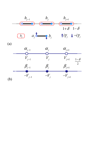
Refer to caption
Figure 1: (Color online) Schematic illustration of the equivalence between imaginary and real potential via non-Hermitian SSH chain in strong dimerization limit. (a) Lattice geometry for the model described in Eq. (1), that represents a non-Hermitian SSH chain with position-dependent $\mathcal{PT}$-symmetric imaginary potential pairs. Solid (empty) circle indicates A (B) lattice, while thin and thick solid lines indicate distorted hopping terms. A $\mathcal{PT}$ dimmer (circled by the red dashed line) contains two strongly coupled sites with opposite imaginary potential (indicated by opposite arrows). (b) Equivalent model described in Eq. (8), that represents two independent uniform chains with opposite position-dependent real potential. If the imaginary potential $i\gamma_{j}$ in (a) is disorder, the real potential $V_{j}$ in (b) is also random distribution, supporting Anderson localization.

We start with the non-Hermitian $\mathcal{PT}$-symmetric dimmer at position $j$, with the Hamiltonian

hj=(1+ฮด)(ajโ€ bj+H.c.)+iฮณj(ajโ€ ajโˆ’bjโ€ bj).h_{j}=(1+\delta)(a_{j}^{{\dagger}}b_{j}+\mathrm{H.c.})+i\gamma_{j}(a_{j}^{{\dagger}}a_{j}-b_{j}^{{\dagger}}b_{j}). (2)

It can be diagonalized as the form

$$h_{j}=\sqrt{(1+\delta)^{2}-\gamma_{j}^{2}}(\overline{\alpha}_{j}\alpha_{j}-\overline{\beta}_{j}\beta_{j}),$$ (3)

by introducing particle operators JL1 ; JL2

{ฮฑj=aj+eโˆ’iโ€‹ฯ†jโ€‹bj1+iโ€‹eโˆ’iโ€‹ฯ†j,ฮฒj=ajโˆ’eiโ€‹ฯ†jโ€‹bj1+iโ€‹eiโ€‹ฯ†jฮฑยฏj=ajโ€ +eโˆ’iโ€‹ฯ†jโ€‹bjโ€ 1โˆ’iโ€‹eโˆ’iโ€‹ฯ†j,ฮฒยฏj=ajโ€ โˆ’eiโ€‹ฯ†jโ€‹bjโ€ 1โˆ’iโ€‹eiโ€‹ฯ†j,casessubscript๐›ผ๐‘—subscript๐‘Ž๐‘—superscript๐‘’๐‘–subscript๐œ‘๐‘—subscript๐‘๐‘—1๐‘–superscript๐‘’๐‘–subscript๐œ‘๐‘—subscript๐›ฝ๐‘—subscript๐‘Ž๐‘—superscript๐‘’๐‘–subscript๐œ‘๐‘—subscript๐‘๐‘—1๐‘–superscript๐‘’๐‘–subscript๐œ‘๐‘—subscriptยฏ๐›ผ๐‘—superscriptsubscript๐‘Ž๐‘—โ€ superscript๐‘’๐‘–subscript๐œ‘๐‘—superscriptsubscript๐‘๐‘—โ€ 1๐‘–superscript๐‘’๐‘–subscript๐œ‘๐‘—subscriptยฏ๐›ฝ๐‘—superscriptsubscript๐‘Ž๐‘—โ€ superscript๐‘’๐‘–subscript๐œ‘๐‘—superscriptsubscript๐‘๐‘—โ€ 1๐‘–superscript๐‘’๐‘–subscript๐œ‘๐‘—\left\{\begin{array}[]{cc}\alpha_{j}=\frac{a_{j}+e^{-i\varphi_{j}}b_{j}}{1+ie^{-i\varphi_{j}}},&\beta_{j}=\frac{a_{j}-e^{i\varphi_{j}}b_{j}}{1+ie^{i\varphi_{j}}}\\ \overline{\alpha}_{j}=\frac{a_{j}^{{\dagger}}+e^{-i\varphi_{j}}b_{j}^{{\dagger}}}{1-ie^{-i\varphi_{j}}},&\overline{\beta}_{j}=\frac{a_{j}^{{\dagger}}-e^{i\varphi_{j}}b_{j}^{{\dagger}}}{1-ie^{i\varphi_{j}}}\end{array}\right., (4)

with

$$\tan\varphi_{j}=\frac{\gamma_{j}}{\sqrt{(1+\delta)^{2}-\gamma_{j}^{2}}}.$$ (5)

Based on the identity

(1+ฮด)โ€‹(ajโ€ โ€‹bj+bjโ€ โ€‹aj)+iโ€‹ฮณjโ€‹(ajโ€ โ€‹ajโˆ’bjโ€ โ€‹bj)1๐›ฟsuperscriptsubscript๐‘Ž๐‘—โ€ subscript๐‘๐‘—superscriptsubscript๐‘๐‘—โ€ subscript๐‘Ž๐‘—๐‘–subscript๐›พ๐‘—superscriptsubscript๐‘Ž๐‘—โ€ subscript๐‘Ž๐‘—superscriptsubscript๐‘๐‘—โ€ subscript๐‘๐‘—\displaystyle(1+\delta)(a_{j}^{{\dagger}}b_{j}+b_{j}^{{\dagger}}a_{j})+i\gamma_{j}(a_{j}^{{\dagger}}a_{j}-b_{j}^{{\dagger}}b_{j}) (6)
$\displaystyle=$ $\displaystyle\sqrt{(1+\delta)^{2}-\gamma_{j}^{2}}(\overline{\alpha}_{j}\alpha_{j}-\overline{\beta}_{j}\beta_{j}),$

and the condition

$$1+\delta\gg 1-\delta,\left|\gamma_{j}\right|\ll 1,$$ (7)

which lead to $\cos\varphi_{j}\approx e^{i\varphi_{j}}\approx 1$, one can neglect the transition terms between sites with opposite potential, and get the approximate expression

$\displaystyle H_{\mathrm{SSH}}$ $\displaystyle\approx$ $\displaystyle\frac{1}{2}(1-\delta)\sum_{j=1}^{N-1}\left(\overline{\alpha}_{j}\alpha_{j+1}-\overline{\beta}_{j}\beta_{j+1}\right)$ (8)
$\displaystyle+\mathrm{H.c.}+\sum_{j=1}^{N}V_{j}(\overline{\alpha}_{j}\alpha_{j}-\overline{\beta}_{j}\beta_{j}).$

The original system reduces to two independent uniform chains with opposite real on-site random potential $V_{j}=\sqrt{(1+\delta)^{2}-\gamma_{j}^{2}}$. Hamiltonian $H_{\mathrm{SSH}}$ is diagonalizable since operators $\left(\alpha_{j},\beta_{j},\overline{\alpha}_{j},\overline{\beta}_{j}\right)$ satisfy the canonical commutation relations. It indicates that $H_{\mathrm{SSH}}$ย can be regarded as a Hermitian model in the context of biorthogonal inner product. On the other hand, we have shown that if a state

|ฯˆโŸฉ=โˆ‘j(Ajโ€‹ฮฑjโ€ โ€‹|0โŸฉ+Bjโ€‹ฮฒjโ€ โ€‹|0โŸฉ),ket๐œ“subscript๐‘—subscript๐ด๐‘—superscriptsubscript๐›ผ๐‘—โ€ ket0subscript๐ต๐‘—superscriptsubscript๐›ฝ๐‘—โ€ ket0\left|\psi\right\rangle=\sum_{j}(A_{j}\alpha_{j}^{{\dagger}}\left|0\right\rangle+B_{j}\beta_{j}^{{\dagger}}\left|0\right\rangle), (9)

with $A_{j}B_{j}=0$ for all $j$, i.e., it has only single-chain component, {ฮฑjโ€ โ€‹|0โŸฉ}superscriptsubscript๐›ผ๐‘—โ€ ket0\left\{\alpha_{j}^{{\dagger}}\left|0\right\rangle\right\} or {ฮฒjโ€ โ€‹|0โŸฉ}superscriptsubscript๐›ฝ๐‘—โ€ ket0\left\{\beta_{j}^{{\dagger}}\left|0\right\rangle\right\}, the dynamics of $\left|\psi\right\rangle$ย is the same as that in a Hermitian chain, exhibiting the standard Anderson localization. Furthermore, the mapping between the Hermitian and non-Hermitian Hamiltonian matrices (i.e., the similar matrix) is a local transformation, which cannot result in localization transition. In conclusion, we provide an example to demonstrate that a nonzero imaginary disorder on-site potential can induce the Anderson localization.

Numerical simulation is performed to demonstrate our conclusion. For simplicity, we consider a uniform chain with disorder potential. The Hamiltonian takes the form

HAnd=โˆ‘lalโ€ โ€‹al+1+H.c.+โˆ‘lฮผlโ€‹alโ€ โ€‹al,formulae-sequencesubscript๐ปAndsubscript๐‘™superscriptsubscript๐‘Ž๐‘™โ€ subscript๐‘Ž๐‘™1Hcsubscript๐‘™subscript๐œ‡๐‘™superscriptsubscript๐‘Ž๐‘™โ€ subscript๐‘Ž๐‘™H_{\text{{And}}}=\sum_{l}a_{l}^{{\dagger}}a_{l+1}+\mathrm{H.c.}+\sum_{l}\mu_{l}a_{l}^{{\dagger}}a_{l}, (10)

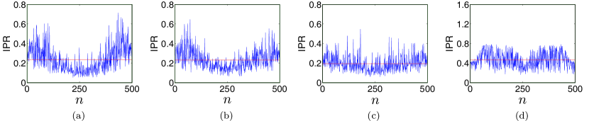
where the potential is simulated by a sequence of random complex variables.ย According to the theory of Anderson localization, all the eigenstates are localized for any nonzero real random variables. On the other hand, our analysis indicates that imaginary random variables may also induce localized states.ย We perform the simulation for two cases, (i) $\mu_{l}=$ ran($-b,b$)$e^{i\phi},$ with $\phi=0$, $\pi/4$, and $\pi/2$, (ii) $\mu_{l}=\mu_{0}e^{i\text{{ran(}}-\pi,\pi\text{{)}}}$. Here $\mathrm{ran}(-b,b)$ย denotes a uniform random number within $(-b,b)$. In case (i) with $\phi=0$, it corresponds to real disorder potential, which is in the framework of Anderson localization. In case (i) with $\phi=\pi/2$, it corresponds to imaginary disorder potential, which is the situation of our prediction. In case (i) with $\phi=\pi/4$, the real and imaginary disorder potential has the same amplitude. In case (ii), the real and imaginary part of potential is out of phase but keep an identical norm.

To characterize the localization natures, we employ the inverse participation ratio (IPR), as a criterion to distinguish the extended states from the localized ones, which is defined as

$$\mathrm{IPR}^{(n)}=\frac{\sum_{l}\left|\left\langle\psi_{n}\right|l\rangle\right|^{4}}{\left(\sum_{l}\left|\left\langle\psi_{n}\right|l\rangle\right|^{2}\right)^{2}}.$$ (11)

Meanwhile, the average IPR (AIPR) for all energy levels is defined as the form of AIPR$=\frac{1}{N}\sum_{n=1}^{N}$IPR(n).ย For spatially extended states, it approaches to zero, whereas it is finite for localized states. For a non-Hermitian system we introduce the quantity, dressed energy

$$\tilde{\varepsilon}_{n}=\mathrm{sgn}[\text{{real}}(\varepsilon_{n})]|\varepsilon_{n}|$$ (12)

to specifies the energy in non-Hermitian regime. We plot the result in Fig. 2, which show that the complex random potential of several types can induce Anderson localization as our prediction.

Refer to caption
Figure 2: (Color online) Numerical simulations for a uniform ring model with random potential sequence $\left\{u_{l}\right\}$. Plots of IPR (blue line) along the energy level index $n$ for four typical sequence $\left\{u_{l}\right\}$, which have the expression $\mu_{l}=$ran($-b,b$)$e^{i\phi}$ with (a) $\phi=0$, (b) $\phi=\frac{\pi}{4}$, (c) $\phi=\frac{\pi}{2}$, and (d) $\mu_{l}=\mu_{0}e^{i\text{{ran(}}-\pi,\pi\text{{)}}}$. The value of AIPR is described by the red line. The system parameters are $N=500$, $u_{0}=2$, $b=2$. It shows that (a), (b), and (c) have similar results, indicating that a complex disorder potential takes the same role as a real one to form Anderson localization. Panel (d) shows a different pattern, which may be due to the different type of expression. Nevertheless the result still accords with our prediction.

III Self-duality under imaginary potential

Consider a uniform chain with imaginary quasiperiodic potential, which has the form

HIm=โˆ‘l=1Nalโ€ โ€‹al+1+H.c.+iโ€‹2โ€‹ฮณโ€‹โˆ‘l=1Ncosโก(qโ€‹l)โ€‹alโ€ โ€‹al,formulae-sequencesubscript๐ปImsuperscriptsubscript๐‘™1๐‘superscriptsubscript๐‘Ž๐‘™โ€ subscript๐‘Ž๐‘™1Hc๐‘–2๐›พsuperscriptsubscript๐‘™1๐‘๐‘ž๐‘™superscriptsubscript๐‘Ž๐‘™โ€ subscript๐‘Ž๐‘™H_{\text{{Im}}}=\sum_{l=1}^{N}a_{l}^{{\dagger}}a_{l+1}+\mathrm{H.c.}+i2\gamma\sum_{l=1}^{N}\mathrm{\cos}(ql)a_{l}^{{\dagger}}a_{l}, (13)

which is an extension from a standard AA model to a non-Hermitian version by extending $\gamma$ย to $i\gamma$, and $q=2\pi\beta$, $\beta$ determines the degree of the quasiperiodicity.ย The simplicity of $H_{\text{{Im}}}$ allows for exact theoretical statements in certain cases. For example, the $1$D disordered Anderson model $H_{\mathrm{And}}$ย with real potential allows for only localized eigenstates at all energies independent of how weak the disorder may be.ย The standard AA model with the $1$D incommensurate potential has either all eigenstates extended or localized depending on the strength of the potential. It is due to the self-duality of the Hamiltonian, which concludes that an AA Hamiltonian with irrational $q$ manifests a localization transition at the self-dual point

$$\left|\gamma\right|=1,$$ (14)

i.e., all eigenstates are extended (localized) when $\left|\gamma\right|<1$ ($\left|\gamma\right|>1$). In the following, it is readily to show that the same thing happens exactly for a non-Hermitian AA model.

Taking the Fourier transformation

$$a_{l}=\frac{1}{\sqrt{N}}\sum_{n}(-1)^{l}e^{iqnl}a_{n},$$ (15)

we can obtain

โˆ’iHIm=ฮณโˆ‘n(anโ€ an+1+H.c.)+2iโˆ‘ncos(qn)anโ€ an.-iH_{\text{{Im}}}=\gamma\sum_{n}(a_{n}^{{\dagger}}a_{n+1}+\mathrm{H.c.})+2i\sum_{n}\cos(qn)a_{n}^{{\dagger}}a_{n}. (16)

Obviously, $H_{\text{{Im}}}$ and $-iH_{\text{{Im}}}$ has the identical complete set of eigenstates and have self-duality with the self-dual point $\gamma=1$. It indicates that the imaginary quasiperiodic potential takes the same role leading to localization transition. Numerical simulations are given in Fig. 3 and Fig. 4 to demonstrate our conclusion about the self-duality under the imaginary potential model.

IV Interference effect on localization transition

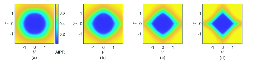
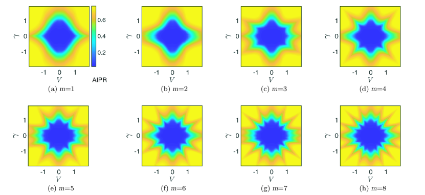
We have seen that a real or imaginary quasiperiodic potential has the same effect on the localization when they show up individually. A natural question is what happens when the quasiperiodic potential is complex. There are many variety of complex potential. In this work, we consider the complex potential with identical frequency

$\displaystyle H_{\mathrm{Comp}}$ $\displaystyle=$ โˆ‘j=1N(ajโ€ aj+1+H.c.)+2Vโˆ‘j=1Ncos(2ฯ€ฮฒj)ajโ€ aj\displaystyle\sum_{j=1}^{N}(a_{j}^{{\dagger}}a_{j+1}+\mathrm{H.c.})+2V\sum_{j=1}^{N}\mathrm{\cos}(2\pi\beta j)a_{j}^{{\dagger}}a_{j} (17)
+iโ€‹2โ€‹ฮณโ€‹โˆ‘j=1Ncosโก(2โ€‹ฯ€โ€‹ฮฒโ€‹j+ฮฆ)โ€‹ajโ€ โ€‹aj,๐‘–2๐›พsuperscriptsubscript๐‘—1๐‘2๐œ‹๐›ฝ๐‘—ฮฆsuperscriptsubscript๐‘Ž๐‘—โ€ subscript๐‘Ž๐‘—\displaystyle+i2\gamma\sum_{j=1}^{N}\mathrm{\cos}(2\pi\beta j+\Phi)a_{j}^{{\dagger}}a_{j},

but different phase difference $\Phi$. In the following, we aim at the effect of $\Phi$ย on the localization transition point. We consider the form of $\Phi$ย in two simple ways. (i) We take the $\Phi$ in the range of $[0,2\pi]$ and it isย ย independent of the values of $V$ and $\gamma$. (ii) Phase difference $\Phi$ is taken as a function of $V$ and $\gamma$, $\Phi=m\tan^{-1}(\gamma/V)$, where $m$ is an integer. We note that the point along $V$ย and $\gamma$ย axes of $\gamma-V$ย plane can be exactly solved as the transition point, i.e., when $|\gamma|<1$ย ($|\gamma|>1$) at $\gamma$ย axis, all the eigenstates are extended (or localized), the same as $\gamma$ย axis but for the point $|V|<1$ย ($|V|>1$) at $V$ย axis. The numerical simulation is performed in the following procedure. For a given point $(V,\gamma)$, we compute the eigenstates by exact diagonalization. Then the IPR of all the levels and the average IPR (AIPR) for all energy levels can be obtained. Meanwhile, we confirm that the maximal and minimal IPR has not much deviations from the average,ย thenย we can use AIPRย to describe the characters of extended (or localized) eigenstates.ย In Figs. 3 and 4, we find that the localization transition boundary is strongly depends on both the magnitude and the phase of the complex potential. The AIPR profiles exhibit interference-like patterns in the parameter space. We also notice that patterns in both figures are asymmetrically under the switch of $V$ and $\gamma$. It is probably due to the Hermiticity of the hopping term, which breaks the balance between the real and imaginary potential.

Refer to caption
Figure 3: (Color online) Color contour maps of the AIPR in the complex $\gamma-V$ plane for the system of Eq. (17)ย with several types of potential configurations. Cause the period of patterns is $\pi/2$, then the simulations are given for the potential with four typical phases (a) $\Phi=0$, (b) $\Phi=\pi/16$, (c) $\Phi=3\pi/16$, and (d) $\Phi=\pi/2$. We see that the AIPR along $V$ and $\gamma$ย axes indicate the localization transition point, which accords with our analysis in Eq. (14). Beyond the axes, the transition point exhibits evident interference pattern. The system parameters are $N=500$, $\beta=(\sqrt{5}-1)/2$.
Refer to caption
Figure 4: (Color online) The same as Fig. 3 but for the system with potential in the expression $\Phi=m\tan^{-1}(\gamma/V)$. Plots of eight typical patterns with integer $m=1,2,3,...,8$, respectively.

V Conclusion

In summary, we have investigated an extension of localization to non-Hermitian system. We have obtained three main results. (i) Based on the equivalence between a disorder non-Hermitian SSH model and a Hermitian uniform chain with real random on-site potential, we have shown exactly that the uncorrelated disorder imaginary on-site potential can induce Anderson localization. (ii) We presented a non-Hermitian AA model, by replacing a real quasiperiodic potential by an imaginary one. It has been shown to have self-duality and thus supports the transition from extension to localization. (iii) Furthermore, we also studied the interactive effect of real and imaginary quasiperiodic potential on the localization transition. Numerical simulations indicates that the phase difference between real and imaginary quasiperiodic potential determines the boundary of transition, exhibiting an interference-like pattern. Our approach opens a new way to investigate the interplay of localization and gain/loss in non-Hermitian system.

Appendix

In this Appendix, we present a detailed derivation for the diagonalization of a non-Hermitian SSH chain with Hamiltonian

HSSH=(1โˆ’ฮด)โ€‹โˆ‘j=1Nโˆ’1bjโ€ โ€‹aj+1+H.c.+โˆ‘j=1Nhj.formulae-sequencesubscript๐ปSSH1๐›ฟsuperscriptsubscript๐‘—1๐‘1superscriptsubscript๐‘๐‘—โ€ subscript๐‘Ž๐‘—1Hcsuperscriptsubscript๐‘—1๐‘subscriptโ„Ž๐‘—H_{\mathrm{SSH}}=(1-\delta)\sum_{j=1}^{N-1}b_{j}^{{\dagger}}a_{j+1}+\mathrm{H.c.}+\sum_{j=1}^{N}h_{j}. (18)

Here each $h_{j}$ย describes a non-Hermitian $\mathcal{PT}$-symmetric dimer

hj=(1+ฮด)(ajโ€ bj+H.c.)+iฮณj(ajโ€ ajโˆ’bjโ€ bj),h_{j}=(1+\delta)(a_{j}^{{\dagger}}b_{j}+\mathrm{H.c.})+i\gamma_{j}(a_{j}^{{\dagger}}a_{j}-b_{j}^{{\dagger}}b_{j}), (19)

at position $j$. It can be diagonalized as the form

$$h_{j}=\sqrt{(1+\delta)^{2}-\gamma_{j}^{2}}(\overline{\alpha}_{j}\alpha_{j}-\overline{\beta}_{j}\beta_{j}),$$ (20)

by introducing canonical particle operators in the aid of biorthogonal inner product. The particle operators

{ฮฑj=aj+eโˆ’iโ€‹ฯ†jโ€‹bj1+iโ€‹eโˆ’iโ€‹ฯ†j,ฮฒj=ajโˆ’eiโ€‹ฯ†jโ€‹bj1+iโ€‹eiโ€‹ฯ†jฮฑยฏj=ajโ€ +eโˆ’iโ€‹ฯ†jโ€‹bjโ€ 1โˆ’iโ€‹eโˆ’iโ€‹ฯ†j,ฮฒยฏj=ajโ€ โˆ’eiโ€‹ฯ†jโ€‹bjโ€ 1โˆ’iโ€‹eiโ€‹ฯ†j,casessubscript๐›ผ๐‘—subscript๐‘Ž๐‘—superscript๐‘’๐‘–subscript๐œ‘๐‘—subscript๐‘๐‘—1๐‘–superscript๐‘’๐‘–subscript๐œ‘๐‘—subscript๐›ฝ๐‘—subscript๐‘Ž๐‘—superscript๐‘’๐‘–subscript๐œ‘๐‘—subscript๐‘๐‘—1๐‘–superscript๐‘’๐‘–subscript๐œ‘๐‘—subscriptยฏ๐›ผ๐‘—superscriptsubscript๐‘Ž๐‘—โ€ superscript๐‘’๐‘–subscript๐œ‘๐‘—superscriptsubscript๐‘๐‘—โ€ 1๐‘–superscript๐‘’๐‘–subscript๐œ‘๐‘—subscriptยฏ๐›ฝ๐‘—superscriptsubscript๐‘Ž๐‘—โ€ superscript๐‘’๐‘–subscript๐œ‘๐‘—superscriptsubscript๐‘๐‘—โ€ 1๐‘–superscript๐‘’๐‘–subscript๐œ‘๐‘—\left\{\begin{array}[]{cc}\alpha_{j}=\frac{a_{j}+e^{-i\varphi_{j}}b_{j}}{1+ie^{-i\varphi_{j}}},&\beta_{j}=\frac{a_{j}-e^{i\varphi_{j}}b_{j}}{1+ie^{i\varphi_{j}}}\\ \overline{\alpha}_{j}=\frac{a_{j}^{{\dagger}}+e^{-i\varphi_{j}}b_{j}^{{\dagger}}}{1-ie^{-i\varphi_{j}}},&\overline{\beta}_{j}=\frac{a_{j}^{{\dagger}}-e^{i\varphi_{j}}b_{j}^{{\dagger}}}{1-ie^{i\varphi_{j}}}\end{array}\right., (21)

with

$$\tan\varphi_{j}=\frac{\gamma_{j}}{\sqrt{(1+\delta)^{2}-\gamma_{j}^{2}}},$$ (22)

or inversely

{aj=(eiโ€‹ฯ†j+i)โ€‹ฮฑj+(eโˆ’iโ€‹ฯ†j+i)โ€‹ฮฒj2โ€‹cosโกฯ†jbj=(1+iโ€‹eโˆ’iโ€‹ฯ†j)โ€‹ฮฑjโˆ’(1+iโ€‹eiโ€‹ฯ†j)โ€‹ฮฒj2โ€‹cosโกฯ†jajโ€ =(eiโ€‹ฯ†jโˆ’i)โ€‹ฮฑยฏj+(eโˆ’iโ€‹ฯ†jโˆ’i)โ€‹ฮฒยฏj2โ€‹cosโกฯ†jbjโ€ =(1โˆ’iโ€‹eโˆ’iโ€‹ฯ†j)โ€‹ฮฑยฏjโˆ’(1โˆ’iโ€‹eiโ€‹ฯ†j)โ€‹ฮฒยฏj2โ€‹cosโกฯ†j,casessubscript๐‘Ž๐‘—superscript๐‘’๐‘–subscript๐œ‘๐‘—๐‘–subscript๐›ผ๐‘—superscript๐‘’๐‘–subscript๐œ‘๐‘—๐‘–subscript๐›ฝ๐‘—2subscript๐œ‘๐‘—subscript๐‘๐‘—1๐‘–superscript๐‘’๐‘–subscript๐œ‘๐‘—subscript๐›ผ๐‘—1๐‘–superscript๐‘’๐‘–subscript๐œ‘๐‘—subscript๐›ฝ๐‘—2subscript๐œ‘๐‘—superscriptsubscript๐‘Ž๐‘—โ€ superscript๐‘’๐‘–subscript๐œ‘๐‘—๐‘–subscriptยฏ๐›ผ๐‘—superscript๐‘’๐‘–subscript๐œ‘๐‘—๐‘–subscriptยฏ๐›ฝ๐‘—2subscript๐œ‘๐‘—superscriptsubscript๐‘๐‘—โ€ 1๐‘–superscript๐‘’๐‘–subscript๐œ‘๐‘—subscriptยฏ๐›ผ๐‘—1๐‘–superscript๐‘’๐‘–subscript๐œ‘๐‘—subscriptยฏ๐›ฝ๐‘—2subscript๐œ‘๐‘—\left\{\begin{array}[]{c}a_{j}=\frac{\left(e^{i\varphi_{j}}+i\right)\alpha_{j}+\left(e^{-i\varphi_{j}}+i\right)\beta_{j}}{2\cos\varphi_{j}}\\ b_{j}=\frac{\left(1+ie^{-i\varphi_{j}}\right)\alpha_{j}-\left(1+ie^{i\varphi_{j}}\right)\beta_{j}}{2\cos\varphi_{j}}\\ a_{j}^{{\dagger}}=\frac{\left(e^{i\varphi_{j}}-i\right)\overline{\alpha}_{j}+\left(e^{-i\varphi_{j}}-i\right)\overline{\beta}_{j}}{2\cos\varphi_{j}}\\ b_{j}^{{\dagger}}=\frac{\left(1-ie^{-i\varphi_{j}}\right)\overline{\alpha}_{j}-\left(1-ie^{i\varphi_{j}}\right)\overline{\beta}_{j}}{2\cos\varphi_{j}}\end{array}\right., (23)

which satisfy the canonical commutation relations

$\displaystyle\left[\alpha_{j},\overline{\alpha}_{j^{\prime}}\right]_{\pm}$ $\displaystyle=$ $\displaystyle\left[\beta_{j},\overline{\beta}_{j^{\prime}}\right]_{\pm}=\delta_{jj^{\prime}},$ (24)
$\displaystyle\left[\alpha_{j},\alpha_{j^{\prime}}\right]_{\pm}$ $\displaystyle=$ $\displaystyle\left[\beta_{j},\beta_{j^{\prime}}\right]_{\pm}=\left[\overline{\alpha}_{j},\overline{\alpha}_{j^{\prime}}\right]_{\pm}=\left[\overline{\beta}_{j},\overline{\beta}_{j^{\prime}}\right]_{\pm}=0,$

for the interchain particles,

$$\left[\alpha_{j},\overline{\beta}_{j^{\prime}}\right]_{\pm}=\left[\overline{\alpha}_{j},\overline{\beta}_{j^{\prime}}\right]_{\pm}=\left[\alpha_{j},\beta_{j^{\prime}}\right]_{\pm}=\left[\overline{\alpha}_{j},\beta_{j^{\prime}}\right]_{\pm}=0,$$ (25)

for the intrachain particles. Straightforward derivations show that

(1+ฮด)โ€‹(ajโ€ โ€‹bj+bjโ€ โ€‹aj)+iโ€‹ฮณjโ€‹(ajโ€ โ€‹ajโˆ’bjโ€ โ€‹bj)1๐›ฟsuperscriptsubscript๐‘Ž๐‘—โ€ subscript๐‘๐‘—superscriptsubscript๐‘๐‘—โ€ subscript๐‘Ž๐‘—๐‘–subscript๐›พ๐‘—superscriptsubscript๐‘Ž๐‘—โ€ subscript๐‘Ž๐‘—superscriptsubscript๐‘๐‘—โ€ subscript๐‘๐‘—\displaystyle(1+\delta)(a_{j}^{{\dagger}}b_{j}+b_{j}^{{\dagger}}a_{j})+i\gamma_{j}(a_{j}^{{\dagger}}a_{j}-b_{j}^{{\dagger}}b_{j}) (26)
$\displaystyle=$ $\displaystyle\sqrt{(1+\delta)^{2}-\gamma_{j}^{2}}(\overline{\alpha}_{j}\alpha_{j}-\overline{\beta}_{j}\beta_{j}),$

and

bjโ€ โ€‹aj+1+aj+1โ€ โ€‹bjsuperscriptsubscript๐‘๐‘—โ€ subscript๐‘Ž๐‘—1superscriptsubscript๐‘Ž๐‘—1โ€ subscript๐‘๐‘—\displaystyle b_{j}^{{\dagger}}a_{j+1}+a_{j+1}^{{\dagger}}b_{j}
$\displaystyle=[\left(e^{i\varphi_{j+1}}+i\right)\left(1-ie^{-i\varphi_{j}}\right)\overline{\alpha}_{j}\alpha_{j+1}$
$\displaystyle+\left(e^{-i\varphi_{j+1}}+i\right)\left(1-ie^{-i\varphi_{j}}\right)\overline{\alpha}_{j}\beta_{j+1}$
$\displaystyle-\left(e^{i\varphi_{j+1}}+i\right)\left(1-ie^{i\varphi_{j}}\right)\overline{\beta}_{j}\alpha_{j+1}$
$\displaystyle-\left(e^{-i\varphi_{j+1}}+i\right)\left(1-ie^{i\varphi_{j}}\right)\overline{\beta}_{j}\beta_{j+1}]\times$
$\displaystyle(4\cos\varphi_{j}\cos\varphi_{j+1})^{-1}+\mathrm{H.c.}.$ (27)

Under the condition

$$1+\delta\gg 1-\delta,\left|\gamma_{j}\right|\ll 1,$$ (28)

we have

$\displaystyle\cos\varphi_{j}$ $\displaystyle=$ $\displaystyle\frac{\sqrt{(1+\delta)^{2}-\gamma_{j}^{2}}}{1+\delta}\approx 1-\frac{\gamma_{j}^{2}}{2(1+\delta)^{2}}\approx 1,$ (29)
$\displaystyle e^{i\varphi_{j}}$ $\displaystyle=$ $\displaystyle\frac{\sqrt{(1+\delta)^{2}-\gamma_{j}^{2}}+i\gamma_{j}}{1+\delta}\approx 1+\frac{i\gamma_{j}}{1+\delta}\approx 1,$ (30)

and then

bjโ€ โ€‹aj+1+aj+1โ€ โ€‹bjsuperscriptsubscript๐‘๐‘—โ€ subscript๐‘Ž๐‘—1superscriptsubscript๐‘Ž๐‘—1โ€ subscript๐‘๐‘—\displaystyle b_{j}^{{\dagger}}a_{j+1}+a_{j+1}^{{\dagger}}b_{j}
$\displaystyle\approx$ $\displaystyle\frac{1}{2}(\overline{\alpha}_{j}\alpha_{j+1}+\overline{\alpha}_{j}\beta_{j+1}-2\overline{\beta}_{j}\alpha_{j+1}-\overline{\beta}_{j}\beta_{j+1})$
+12โ€‹(ฮฑj+1โ€ โ€‹ฮฑยฏjโ€ โˆ’ฮฑj+1โ€ โ€‹ฮฒยฏjโ€ +ฮฒj+1โ€ โ€‹ฮฑยฏjโ€ โˆ’ฮฒj+1โ€ โ€‹ฮฒยฏjโ€ )12superscriptsubscript๐›ผ๐‘—1โ€ superscriptsubscriptยฏ๐›ผ๐‘—โ€ superscriptsubscript๐›ผ๐‘—1โ€ superscriptsubscriptยฏ๐›ฝ๐‘—โ€ superscriptsubscript๐›ฝ๐‘—1โ€ superscriptsubscriptยฏ๐›ผ๐‘—โ€ superscriptsubscript๐›ฝ๐‘—1โ€ superscriptsubscriptยฏ๐›ฝ๐‘—โ€ \displaystyle+\frac{1}{2}(\alpha_{j+1}^{{\dagger}}\overline{\alpha}_{j}^{{\dagger}}-\alpha_{j+1}^{{\dagger}}\overline{\beta}_{j}^{{\dagger}}+\beta_{j+1}^{{\dagger}}\overline{\alpha}_{j}^{{\dagger}}-\beta_{j+1}^{{\dagger}}\overline{\beta}_{j}^{{\dagger}})
$\displaystyle=$ $\displaystyle\frac{1}{2}(\overline{\alpha}_{j}\alpha_{j+1}+\overline{\alpha}_{j}\beta_{j+1}-\overline{\beta}_{j}\alpha_{j+1}-\overline{\beta}_{j}\beta_{j+1})+\mathrm{H.c.}.$

Neglecting the transition terms between sites with opposite potential, we have

bjโ€ โ€‹aj+1+aj+1โ€ โ€‹bjโ‰ˆ12โ€‹ฮฑยฏjโ€‹ฮฑj+1โˆ’12โ€‹ฮฒยฏjโ€‹ฮฒj+1+H.c..formulae-sequencesuperscriptsubscript๐‘๐‘—โ€ subscript๐‘Ž๐‘—1superscriptsubscript๐‘Ž๐‘—1โ€ subscript๐‘๐‘—12subscriptยฏ๐›ผ๐‘—subscript๐›ผ๐‘—112subscriptยฏ๐›ฝ๐‘—subscript๐›ฝ๐‘—1Hcb_{j}^{{\dagger}}a_{j+1}+a_{j+1}^{{\dagger}}b_{j}\approx\frac{1}{2}\overline{\alpha}_{j}\alpha_{j+1}-\frac{1}{2}\overline{\beta}_{j}\beta_{j+1}+\mathrm{H.c.}. (32)

Then we have the approximate expression

$\displaystyle H_{\mathrm{SSH}}$ $\displaystyle\approx$ $\displaystyle\frac{1}{2}(1-\delta)\sum_{j=1}^{N-1}\left(\overline{\alpha}_{j}\alpha_{j+1}-\overline{\beta}_{j}\beta_{j+1}\right)$ (33)
$\displaystyle+\mathrm{H.c.}+\sum_{j=1}^{N}V_{j}(\overline{\alpha}_{j}\alpha_{j}-\overline{\beta}_{j}\beta_{j}),$

where real potential $V_{j}=\sqrt{(1+\delta)^{2}-\gamma_{j}^{2}}$. On the other hand, we have

[ฮฑj,ฮฑjโ€ฒโ€ ]ยฑsubscriptsubscript๐›ผ๐‘—superscriptsubscript๐›ผsuperscript๐‘—โ€ฒโ€ plus-or-minus\displaystyle\left[\alpha_{j},\alpha_{j^{\prime}}^{{\dagger}}\right]_{\pm} $\displaystyle=$ ฮดjโ€‹jโ€ฒ1+sinโกฯ†j,[ฮฒj,ฮฒjโ€ฒโ€ ]ยฑ=ฮดjโ€‹jโ€ฒ1โˆ’sinโกฯ†j,subscript๐›ฟ๐‘—superscript๐‘—โ€ฒ1subscript๐œ‘๐‘—subscriptsubscript๐›ฝ๐‘—superscriptsubscript๐›ฝsuperscript๐‘—โ€ฒโ€ plus-or-minussubscript๐›ฟ๐‘—superscript๐‘—โ€ฒ1subscript๐œ‘๐‘—\displaystyle\frac{\delta_{jj^{\prime}}}{1+\sin\varphi_{j}},\left[\beta_{j},\beta_{j^{\prime}}^{{\dagger}}\right]_{\pm}=\frac{\delta_{jj^{\prime}}}{1-\sin\varphi_{j}}, (34)
$\displaystyle\left[\alpha_{j},\alpha_{j^{\prime}}\right]_{\pm}$ $\displaystyle=$ [ฮฒj,ฮฒjโ€ฒ]ยฑ=[ฮฑjโ€ ,ฮฑjโ€ฒโ€ ]ยฑ=[ฮฒjโ€ ,ฮฒjโ€ฒโ€ ]ยฑ=0,subscriptsubscript๐›ฝ๐‘—subscript๐›ฝsuperscript๐‘—โ€ฒplus-or-minussubscriptsuperscriptsubscript๐›ผ๐‘—โ€ superscriptsubscript๐›ผsuperscript๐‘—โ€ฒโ€ plus-or-minussubscriptsuperscriptsubscript๐›ฝ๐‘—โ€ superscriptsubscript๐›ฝsuperscript๐‘—โ€ฒโ€ plus-or-minus0\displaystyle\left[\beta_{j},\beta_{j^{\prime}}\right]_{\pm}=\left[\alpha_{j}^{{\dagger}},\alpha_{j^{\prime}}^{{\dagger}}\right]_{\pm}=\left[\beta_{j}^{{\dagger}},\beta_{j^{\prime}}^{{\dagger}}\right]_{\pm}=0,

for the interchain particles,

[ฮฑj,ฮฒjโ€ฒโ€ ]ยฑsubscriptsubscript๐›ผ๐‘—superscriptsubscript๐›ฝsuperscript๐‘—โ€ฒโ€ plus-or-minus\displaystyle\left[\alpha_{j},\beta_{j^{\prime}}^{{\dagger}}\right]_{\pm} $\displaystyle=$ iโ€‹tanโกฯ†jโ€‹ฮดjโ€‹jโ€ฒ,[ฮฑjโ€ ,ฮฒjโ€ฒ]ยฑ=โˆ’iโ€‹tanโกฯ†jโ€‹ฮดjโ€‹jโ€ฒ,๐‘–subscript๐œ‘๐‘—subscript๐›ฟ๐‘—superscript๐‘—โ€ฒsubscriptsuperscriptsubscript๐›ผ๐‘—โ€ subscript๐›ฝsuperscript๐‘—โ€ฒplus-or-minus๐‘–subscript๐œ‘๐‘—subscript๐›ฟ๐‘—superscript๐‘—โ€ฒ\displaystyle i\tan\varphi_{j}\delta_{jj^{\prime}},\left[\alpha_{j}^{{\dagger}},\beta_{j^{\prime}}\right]_{\pm}=-i\tan\varphi_{j}\delta_{jj^{\prime}},
$\displaystyle\left[\alpha_{j},\beta_{j^{\prime}}\right]_{\pm}$ $\displaystyle=$ [ฮฑjโ€ ,ฮฒjโ€ฒโ€ ]ยฑ=0,subscriptsuperscriptsubscript๐›ผ๐‘—โ€ superscriptsubscript๐›ฝsuperscript๐‘—โ€ฒโ€ plus-or-minus0\displaystyle\left[\alpha_{j}^{{\dagger}},\beta_{j^{\prime}}^{{\dagger}}\right]_{\pm}=0, (35)

for the intrachain particles. It indicates that if a state satisfy theย relation

|ฯˆโŸฉ=โˆ‘j(Ajโ€‹ฮฑjโ€ โ€‹|0โŸฉ+Bjโ€‹ฮฒjโ€ โ€‹|0โŸฉ),ket๐œ“subscript๐‘—subscript๐ด๐‘—superscriptsubscript๐›ผ๐‘—โ€ ket0subscript๐ต๐‘—superscriptsubscript๐›ฝ๐‘—โ€ ket0\left|\psi\right\rangle=\sum_{j}(A_{j}\alpha_{j}^{{\dagger}}\left|0\right\rangle+B_{j}\beta_{j}^{{\dagger}}\left|0\right\rangle), (36)

with $A_{j}B_{j}=0$ for all $j$, i.e., it has only single-chain component, {ฮฑjโ€ โ€‹|0โŸฉ}superscriptsubscript๐›ผ๐‘—โ€ ket0\left\{\alpha_{j}^{{\dagger}}\left|0\right\rangle\right\} or {ฮฒjโ€ โ€‹|0โŸฉ}superscriptsubscript๐›ฝ๐‘—โ€ ket0\left\{\beta_{j}^{{\dagger}}\left|0\right\rangle\right\}, the dynamics of $\left|\psi\right\rangle$ย is the same as that in a Hermitian chain.

Acknowledgements.
We acknowledge the support of NSFC (Grants No. 11874225).

References

  • (1) Patrick A. Lee and T. V. Ramakrishnan, Disordered electronic systems, Rev. Mod. Phys. 57, 287 (1985).
  • (2) Schwartz T., Bartal G., Fishman S. and Segev M., Transport and Anderson localization in disordered two-dimensional photonic lattices, Nature, 446, 52 (2007).
  • (3) S. Gentilini, A. Fratalocchi, L. Angelani, G. Ruocco, and C. Conti, Ultrashort pulse propagation and the Anderson localization, Opt. Lett. 34, (2009).
  • (4) C. Conti and A. Fratalocchi, Dynamic light diffusion, three-dimensional Anderson localization and lasing in inverted opals, Nat. Phys., 4, 794-798 (2008).
  • (5) Diego Molinari and Andrea Fratalocchi, Route to strong localization of light: the role of disorder, Opt. Express, 20, 18156-18164 (2012).
  • (6) Klaus Drese and Martin Holthaus, Exploring a Metal-Insulator Transition with Ultracold Atoms in Standing Light Waves? Phys. Rev. Lett., 78, 2932 (1997).
  • (7) Giacomo Roati, Chiara Dโ€™Errico, Leonardo Fallani, Marco Fattori, Chiara Fort, Matteo Zaccanti, Giovanni Modugno, Michele Modugno and Massimo Inguscio, Anderson localization of a non-interacting Boseโ€“Einstein condensate, Nature, 453, 895-898 (2008).
  • (8) F. Jendrzejewski, A. Bernard, K. Mรผler, P. Cheinet, V. Josse, M. Piraud, L. Pezzรฉ, L. Sanchez-Palencia, A. Aspect and P. Bouyer, Three-dimensional localization of ultracold atoms in an optical disordered potential, Nat. Phys. 8, 398-403 (2012).
  • (9) G. Semeghini, M. Landini, P. Castilho, S. Roy, G. Spagnolli, A. Trenkwalder, M. Fattori, M. Inguscio and G. Modugno, Measurement of the mobility edge for 3D Anderson localization, Nat. Phys. 11, 554-559 (2015).
  • (10) Hefei Hu, A. Strybulevych, J. H. Page, S. E. Skipetrov and B. A. van Tiggelen, Localization of ultrasound in a three-dimensional elastic network, Nat. Phys., 4, 945-948 (2008).
  • (11) Julien Chabรฉ, Gabriel Lemariรฉ Benoรฎt Grรฉaud, Dominique Delande, Pascal Szriftgiser, and Jean Claude Garreau, Experimental Observation of the Anderson Metal-Insulator Transition with Atomic Matter Waves, Phys. Rev. Lett., 101 255702 (2008).
  • (12) P. W. Anderson, Absence of Diffusion in Certain Random Lattices, Phys. Rev., 109, 1492 (1958).
  • (13) M. Ya. Azbel, Quantum Particle in One-Dimensional Potentials with Incommensurate Periods, Phys. Rev. Lett. 43, 1954 (1979)
  • (14) Serge Aubry and G. Andre, Analyticity Breaking and Anderson Localization in Incommensurate Lattices, Ann. Isr. Phys. Soc. 3, 133 (1980).
  • (15) Luca Dal Negro, Claudio J. Oton, Zeno Gaburro, Lorenzo Pavesi, Patrick Johnson, Ad Lagendijk, Roberto Righini, Marcello Colocci, and Diederik S. Wiersma, Light Transport through the Band-Edge States of Fibonacci Quasicrystals, Phys. Rev. Lett. 90, 055501 (2003).
  • (16) L. Fallani, J. E. Lye, V. Guarrera, C. Fort, and M. InguscioL, Ultracold Atoms in a Disordered Crystal of Light: Towards a Bose Glass, Phys. Rev. Lett. 98, 130404 (2007).
  • (17) Y. Lahini, R. Pugatch, F. Pozzi, M. Sorel, R. Morandotti, N. Davidson, and Y. Silberberg, Observation of a Localization Transition in Quasiperiodic Photonic Lattices, Phys. Rev. Lett. 103, 013901 (2009).
  • (18) Giovanni Modugno, Anderson Localization in Boseโ€“Einstein Condensates, Rep. Prog. Phys. 73, 102401 (2010).
  • (19) Mordechai Segev, Yaron Silberberg, and Demetrios N. Christodoulides, Anderson Localization of Light, Nat. Photonics 7, 197-204 (2013).
  • (20) L. Jin and Z. Song, Incident Direction Independent Wave Propagation and Unidirectional Lasing, Phys. Rev. Lett. 121, 073901 (2018).
  • (21) A. Metelmann and A. A. Clerk, Nonreciprocal Photon Transmission and Amplification via Reservoir Engineering, Phys. Rev. X 5, 021025 (2015).
  • (22) H. Ramezani, P. K. Jha, Y. Wang, and X. Zhang, Nonreciprocal Localization of Photons, Phys. Rev. Lett. 120, 043901 (2018).
  • (23) T. T. Koutserimpas and R. Fleury, Nonreciprocal Gain in Non-Hermitian Time-Floquet Systems, Phys. Rev. Lett. 120, 087401 (2018).
  • (24) R. Huang, A. Miranowicz, J.-Q. Liao, F. Nori, and H. Jing, Nonreciprocal Photon Blockade, Phys. Rev. Lett. 121, 153601 (2018).
  • (25) Carl M Bender, Making sense of non-Hermitian Hamiltonians, Rep. Prog. Phys. 70, 947 (2007).
  • (26) Z. H. Musslimani, K. G. Makris, R. El-Ganainy, and D. N. Christodoulides, Optical Solitons in PT Periodic Potentials, Phys. Rev. Lett. 100, 030402 (2008).
  • (27) K. G. Makris, R. El-Ganainy, D. N. Christodoulides, and Z. H. Musslimani, Beam Dynamics in PT Symmetric Optical Lattices, Phys. Rev. Lett. 100, 103904 (2008).
  • (28) S. Klaiman, U. Gรผnther, and N. Moiseyev, Visualization of Branch Points in PT-Symmetric Waveguides, Phys. Rev. Lett. 101, 080402 (2008).
  • (29) Y. D. Chong, L. Ge, H. Cao, and A. D. Stone, Coherent perfect absorbers: time-reversed lasers, Phys. Rev. Lett. 105, 053901 (2010).
  • (30) C. E. Rรผter et al., Observation of parity-time symmetry in optics, Nat. Phys. 6, 192 (2010).
  • (31) A. Regensburger, C. Bersch, M.-A. Miri, G. Onishchukov, D. N. Christodoulides, and U. Peschel, Parity-time synthetic photonic lattices Nature 488, 167 (2012).
  • (32) Liang Feng, Ye-Long Xu, William S. Fegadolli, Ming-Hui Lu, Josรฉ E. B. Oliveira, Vilson R. Almeida, Yan-Feng Chen, and Axel Scherer, Experimental demonstration of a unidirectional reflectionless parity-time metamaterial at optical frequencies, Nature Mater. 12, 108-113 (2013).
  • (33) R. Fleury, D. Sounas, and A. Alรน, An invisible acoustic sensor based on parity-time symmetry, Nat. Commun. 6, 5905 (2015).
  • (34) N. Moiseyev, Non-Hermitian Quantum Mechanics (Cambridge Univ. Press, 2011).
  • (35) L. Feng, R. El-Ganainy, and L. Ge, Non-Hermitian photonics based on parityโ€“time symmetry, Nat. Photo. 11, 752 (2017).
  • (36) R. El-Ganainy, K. G. Makris, M. Khajavikhan, Z. H. Musslimani, S. Rotter, and D. N. Christodoulides, Non-Hermitian physics and $\mathcal{PT}$ symmetry, Nat. Phys. 14, 11 (2018).
  • (37) S. K. Gupta, Y. Zou, X.-Y. Zhu, M.-H. Lu, L. Zhang, X.-P. Liu, and Y.-F. Chen, Parity-time Symmetry in Non-Hermitian Complex Media, arXiv:1803.00794.
  • (38) D. Christodoulides and J. Yang, Parity-time Symmetry and Its Applications (Springer, 2018).
  • (39) C. Yuce, $\mathcal{PT}$ symmetric Aubryโ€“Andre model, Phys. Lett. A 378, 2024-2028 (2014).
  • (40) S. Longhi, Topological Phase Transition in non-Hermitian Quasicrystals, Phys. Rev. Lett. 122, 237601 (2019).
  • (41) S. Longhi, Metal-insulator phase transition in a non-Hermitian Aubry-Andre-Harper Model, arXiv:1908.03371.
  • (42) L. Jin and Z. Song, Solutions of $\mathcal{PT}$-symmetric tight-binding chain and its equivalent Hermitian counterpart, Phys. Rev. A 80, 052107 (2009).
  • (43) L. Jin and Z. Song, Scaling behavior and phase diagram of a PT -symmetric non-Hermitian Boseโ€“Hubbard system,ย Annals of Physics 330 142โ€“159ย (2013).