Coin_flipper at eHealth-KD Challenge 2019

Abstract

This paper describes our approach presented for the eHealth-KD 2019 challenge. Our participation was aimed at testing how far we could go using generic tools for Text-Processing but, at the same time, using common optimization techniques in the field of Data Mining. The architecture proposed for both tasks of the challenge is a standard stacked 2-layer bi-LSTM. The main particularities of our approach are: (a) The use of a surrogate function of F1 as loss function to close the gap between the minimization function and the evaluation metric, and (b) The generation of an ensemble of models for generating predictions by majority vote. Our system ranked second with an F1 score of 62.18% in the main task by a narrow margin with the winner that scored 63.94%.

1 Introduction

This article describes the model presented by the coin-flipper team for solving the shared task presented in eHealth-KD 2019 challenge [10]. The main goal of the challenge is to encourage the development of software systems to automatically extract information from electronic health documents written in Spanish. The challenge involves two subtasks: 1) Identification and classification of key phrases (four different types of units) and 2) Detection of semantic relations among them (thirteen semantic relations).

The tasks proposed are similar to previous competitions such as Semeval-2017 Task 10: ScienceIE [1] and TASS-2018-Task 3 eHealth Knowledge Discovery [3], but the types of entities and the amount of semantic relations to be identified have been changing over time. Also, we find changes in the systems approaches evolving from rule based methods to Deep Learning models some of them incorporating domain-specific knowledge.

As the organizers of the challenge state, although this challenge is oriented to the health domain, the kind of knowledge to be extracted is general-purpose. With this idea in mind, we propose a model that avoids the use of knowledge or tools specific to the domain, easing the portability of the model to new domains and tasks.

2 Tasks and data

The eHealth-KD 2019 challenge involves two subtasks: subtask A) Identification and classification of key phrases (four different types of units), and subtask B) Detection of semantic relations among them (thirteen semantic relations).

Each subtask has been evaluated individually and also as components of a pipeline. For this purpose, three evaluation scenarios have been proposed. Scenario 1 requires subtasks A and B to be executed sequentially in a pipeline. Scenario 2 only evaluates subtask A and Scenario 3 only evaluates subtask B.

A training set that contains a total of 600 sentences was provided to be used for the learning step. For the validation step, an additional set of 100 sentences was available.

A detailed explanation of the corpus data, subtasks and evaluation metrics can be found in the overview description paper [10].

3 Our approach

Our aim was to see how far we can get in tasks described above using generic NLP tools (non-specific for the domain) and standard Data Mining strategies.

About the model to be learned, given the sequential nature of the data (sentences), we proposed a stacked 2-layer bi-LSTM architecture. LSTMs have been proved a successful approach in several Natural Language Processing tasks, such as Named Entity Recognition (f.i. [8]) and Semantic Role Labeling (f.i. [12]). About the data mining strategies, we applied two following strategies:

1. Building an ensemble of models for generating predictions:

   It is well known in Machine Learning that ensemble models have higher performance than single models [13], specially when models have a high variance which is the case of neural networks. So, for each task, we build an ensemble of models instead of a single model.

   There are several ways to generate an ensemble of neural networks. Usually, differences in hyperparameters or different architectures are enough to ensure diversity of models necessary for making ensemble methods profitable. In our case we achieve diversity by using random initialization of models before training [6].

   There also exist a lot of different techniques to combine the output of different models into a single prediction [13]. We will apply the simplest method of majority vote to combine the outputs of the models in a ensemble.

2. The use of a surrogate function of F1 metric as the loss function:

   Usually, accuracy is the metric to be optimized and Cross-entropy (CE) is the continuous function used as loss function. However, in this challenge, F1 score is used for evaluation. The use of CE is not optimal in this case because we would like to minimize the error according to the metric used for evaluation. In [5], authors propose to solve this problem by defining continuous surrogate upper and lower bounds for true positive and false positive cases and, from them, F1’ surrogate. Then they use $1/{F1^{\prime}}$ as the loss function to minimize. We have done it differently: in our case, getting the predictions $\hat{y}$ from our Neural Network (with sigmoid function activation in last layer), we choose to use a soft version of F1 metric. We define soft-true positive cases ($tp_{s}$) and soft-false positives ($fp_{s}$), where labels $y$ are in {0,1} and predictions $\hat{y}$ in [0..1], as:

   $$tp_{s} =\sum_{i\in Y^{+}}\hat{y}_{i}=\sum_{i\in Y}y_{i}\hat{y}_{i}$$

   $$fp_{s} =\sum_{i\in Y^{-}}\hat{y}_{i}=\sum_{i\in Y}(1-y_{i})\hat{y}_{i}$$

   Notice that when predicted labels $\hat{y}$ are hard (0 or 1), these values are exactly true and false positive cases, respectively.

   Replacing soft versions of true and false positives cases in F1 definition (in the type I and type II error form), we have our surrogate $F1_{s}$ function to maximize.

   $$F1_{s}\;=\;\frac{2\;tp_{s}}{\left|Y^{+}\right|+tp_{s}+fp_{s}}\;=\;\frac{2\;\sum_{i\in Y^{+}}\hat{y}_{i}}{\left|Y^{+}\right|+\sum_{i\in Y^{+}}\hat{y}_{i}+\sum_{i\in Y^{-}}\hat{y}_{i}}$$ (1)

   Note that maximize $F1_{s}$ implies increasing $\hat{y}$ of positive cases while decreasing $\hat{y}$ of negative cases in a proportional way to F1 function. Loss function to minimize will be $1-F1_{s}$.

In the next sections we describe further details about how subtasks A and B are solved.

3.1 Subtask A

Subtask A consists in detecting key phrases in texts (from now on we will abbreviate key phrase to KPhr) and their kind or class. For this task we set as input only the sequence of words of each sentence and their Part-of-Speech (PoS). Words are represented using FastText embeddings [2] trained on the Spanish Billion Word Corpus [4]. Among the advantages of FastText over other approaches are that, being FastText trained on n-grams of words, embeddings carry implicitly morphological information and also are able to output a reasonable embedding for a word not seen during training.

PoS for sentences are generated using spaCy[7] tagger for Spanish. Probably better results would be obtained using more advanced taggers like FreeLing PoS tagger [9].

In the definition of the output of the architecture we were inspired on image segmentation work in which, given an image, a mask over the image is generated that encodes for each pixel the class it belongs to. Similarly, for each sentence, we define as output a mask vector where for each word we have codified the kind of KPhr the word belongs to (or a label denoting that the word does not belong to any KPhr).

The architecture of the model to be learned consists of two stacked layers of bi-LSTM feed with the word embedding and the one-hot encoding of the PoS for each word of the sentence. We apply sequence Padding (with length parameter equal to the length of the larger sentence in data set) and Masking. Initially, output was defined as a vector with the one-hot codification of the corresponding KPhr label for each word. However, we found empirically that learning a model to predict all kinds of KPhr was not very successful. So, we decided to split the task into learning models specialized in predictions for each kind of KPhr. With this modification, now the output of the architecture is a 0/1 vector with 1 denoting if a word belongs to the kind of KPhr the model is trained for, and 0 otherwise. Notice that with this modification, the use of F1 loss become even more important because the induced sparsity of labels.

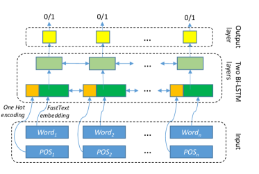
Figure 1: Basic two level bi-LSTM architecture for subtask A. Input are words and their PoS that are embedded using FastText and one-hot encoding, respectively. For each kind of key phrase we train a separate ensemble of 15 models. Output in subtask A is 0/1 with 1 denoting the current word belongs to a key phrase of the kind we are training for, and 0 otherwise.

The learning of each model is done by using surrogate $1-F1_{s}$ loss (as explained in previous section) with early stopping when $F1$ score does not improve in 100 epochs on the development dataset, and returning the model that reaches the best $F1$ score on development dataset. Default learning rate $0.001$ with adam optimization is used. Batch size is 32 sentences. Neither dropout nor data augmentation is used. First bi-LSTM layer has 150 units in each direction. Second bi-LSTM layer has 32 units in each direction. The same architecture is used for all KPhr detection models without fine-tuning of parameters. See a graphical representation of the model in Figure 1.

As stated in the previous section, we create an ensemble of 15 models for each target KPhr that is used later to generate the final prediction by majority voting. Diversity of models in the ensemble is obtained only from different initialization of weights. To avoid the vote of specially bad models, each model is applied to the development dataset and those models with an F1 score far below the average of the ensemble are removed from it.

Our approach has two obvious problems. The first one is that, because the way we define segmentation, we don’t know when a KPhr starts nor ends. A naive solution would be to join into the same KPhr consecutive words that are tagged with the same label. However this heuristic solution does not always work. We solve this problem by inspecting the PoS of consecutive words tagged with the same label. For each combination of PoS found, we compute how many cases covered are in fact cases where words belong to the same KPhr. From the statistics of these cases we create a set of rules that decide if two consecutive words with the same label really belong to the same KPhr or not.

The second problem is that having different models, one for each kind of KPhr, words could be labeled as belonging to different kinds of KPhr at the same time. So, in case of conflict among different ensembles, in order to decide the final kind of KPhr, we count how many positive votes each ensemble has emitted and multiply it by a weighting parameter. The ensemble with the highest product is the winner and the word is labeled with the kind of KPhr the ensemble represents. Weights for each ensemble are found by applying the ensembles on the development dataset and grid-searching for the combination of weights that returns highest global F1.

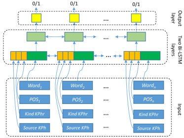
Figure 2: Two layer bi-LSTM architecture for subtask B detecting relation rel. Given a source KPhr (identified in subtask A), output consists of 0/1 with 1 denoting if the current word belongs to a KPhr that is target of rel for the source KPhr. Input consists of (for each word of the sentence) the word, PoS tag, kind of KPhr the word belongs to (if any) and, finally, if current word belongs to source KPhr or not. Words and PoS are embedded as in subtask A, and all other information is embedded using one-hot encoding.

3.2 Subtask B

Subtask B consists in detecting semantic relations (thirteen types of relations) between KPhr pairs identified in the previous task. For this task, given a relation rel and a KPhr considered as source for the relation, we try to identify another KPhr in the sentence with the role target for this relation rel. In order to learn models able to solve this task, we define an architecture that, given a relation rel and a source KPhr, has the following inputs:

1. Sequence of words in the sentence where source KPhr is found.

2. Part of Speech tags for each word in the sentence.

3. Mask denoting for each word the kind of KPhr it belongs to (codifying in 1-4 the kind of KPhr and 0 if it does not belong to any KPhr).

4. 0/1 Mask vector for each word with 1 denoting if the word belongs to the source KPhr, and 0 otherwise.

Words are represented as FastText vector embeddings and all other inputs are encoded using one-hot encoding. All vectors codifying the information of one word are concatenated. See Figure 2 for a representation of the architecture.

For each relation we build a Neural Network that consists of the embedding layers explained above plus 2 stacked bi-LSTM layers. As in subtask A, we use padding and masking. The output consists of a mask vector 0/1 with 1 only for those words who belong to a target KPhr of the relation rel of current KPhr as source. When no target KPhr exists for the current relation, output is all zeros.

When the model identifies at least one word of a target KPhr, we consider the whole KPhr detected. The output representation selected allows that in the same sentence one KPhr as source has several KPhr as target for the same relation.

All training parameters and procedures are the same as those used in subtask A. Again, the learning of each model is done by using surrogate $1-F1_{s}$ loss with early stopping when $F1$ score does not improve in 100 epochs on the development dataset, and returning the model that reaches the best $F1$ score on development dataset. Default learning rate $0.001$ with adam optimization is used. Batch size is 32. Neither dropout nor data augmentation is used. First bi-LSTM layer has 150 units in each direction. Second bi-LSTM layer has 32 units in each direction. The same architecture is used for all relations without fine-tuning of parameters. For each relation, an ensemble of 15 models is built from which majority voting is implemented.

In some cases, ensembles of different relations identify the same pair of KPhr as positive cases. When this happens, we assign to the pair of KPhr the relation of the ensemble with highest precision on the development dataset.

4 Results

Table 1 shows F1 scores for the three scenarios achieved by the baseline system provided by organizers, the best method and our method.

Our results were very competitive. We were second in the main evaluation (scenario 1) by a narrow margin - only 1.76 of F1 score over 100. In scenario 2 and, specially, scenario 3 we were at a larger distance to the best method (see Table 1) in positions 5th and 4th of the ranking, respectively. This is surprising because scenario 1 is the composition of the other 2 scenarios. The main difference in evaluation among scenarios was that for scenario 1 a subset of 100 sentences out of a 8.800 sentences dataset was randomly selected for evaluation, while in scenarios 2 and 3 a dataset of 100 sentences was given to each one for evaluation.

For scores shown in Table 1 we did not submit results for different parameters except for subtask B. In subtask B, we noticed that not all relations had the same difficulty in being detected. We found that a first set of 6 relations (in-context, subject, target, domain, arg and is-a) were successfully identified with high recall and precision values when tested on development dataset (above 75%). Relations in-place, has-property, same-as and in-time were (in this order) harder to identify and, finally, for part-of, causes and entails relations, results were so bad that models for those relations were discarded.

In order to obtain the highest score, we ranked relations by their F1 scores on development dataset and submitted different sets of results considering only relations that were in 6, 7, 8, 9 and 10 top positions. Best results on testing dataset were obtained considering top 7 relations, that is, the ones in the first set (in-context, subject, target, domain, arg and is-a) plus in-place. Considering only a subset of possible relations had an obvious impact on final performance that achieved good precision but low recall.

We think that difficulty in detecting relations part-of, same-as, in-time, entails and has-property comes from the low number of instances (range 50-100) in the training set. So, for these cases, some techniques like data augmentation should be used to obtain better results. An exception is relation causes that had 230 instances and was very difficult to identify with our approach. In this case most complex architectures should be used.

Table 1: F1 scores, Precision and Recall obtained for the three scenarios achieved by baseline system, best method presented and our method.

  baseline Joint-BERT-RCNN (best) Voting LSTMs (ours) F1 P R F1   P R F1 P R   scenario 1 43.09 52.04 36.77 63.94   65.06 62.86 62.18 74.54 53.34 scenario 2 54.66 51.29 58.51 82.03   80.73 83.36 78.73 79.86 77.63 scenario 3 12.31 48.78 7.04 62.69   66.67 59.15 49.31 71.33 37.68

5 Conclusions

In this paper we have presented a simple approach to solve the tasks proposed in this competition. The aim was to measure how far we can get with standard tools and simple algorithms but using common optimization techniques in the Data Mining field. In particular, the architecture proposed for both tasks was a two level bi-LSTM to modelize each of the classes we wanted to capture. We didn’t use state of the art language models like BERT, ELMO or GPT, neither specialized NER techniques, knowledge bases or taggers specific for the domain (so results probably will be similar in other domains).

The main particularities of our approach are: (a) The use of a surrogate loss function of F1 metric to close the gap between the minimization function and the evaluation metric and (b) the generation of an ensemble of models for generating predictions by majority vote.

From results, we conclude that it is worth using the evaluation metric (or a surrogate function of it) as loss function and also building ensemble models for generating predictions. We did not do an exhaustive study of the improvement in performance due to the use of a surrogate function of F1 as loss, but in initial experiments we found a clear advantage of the surrogate function usage instead of standard loss functions. We neither did an exhaustive study of the impact in performance of learning ensemble models instead of learning single models, however, we noticed that usually F1 scores obtained by the majority vote of the ensemble was about 1-2 points higher than the best model of the ensemble and 3-4 points higher than the average of the models of the ensemble. Note that combination of outputs in the ensemble is made through simple majority voting but more complex ensemble techniques could improve the performance of the system even more. For a review of ensemble methods see [13].

The results show that our model achieves good precision scores for the three scenarios but sometimes at the expense of lower recall levels than other systems, specially notorious in scenario 3. The difficulties our model had in identifying some semantic relations may be due to the low number of examples of these relations in the training dataset. To deal with this problem, we are planning to use data augmentation techniques in order to increase the number of instances of the less frequent relations. One of the techniques we want to explore is backtranslation, used in text classification [11].

References

- [1] Augenstein, I., Das, M., Riedel, S., Vikraman, L., McCallum, A.: SemEval 2017 Task 10: ScienceIE - Extracting Keyphrases and Relations from Scientific Publications. In: Proceedings of the 11th International Workshop on Semantic Evaluation (SemEval-2017). pp. 546–555 (2017). https://doi.org/10.18653/v1/S17-2091
- [2] Bojanowski, P., Grave, E., Joulin, A., Mikolov, T.: Enriching Word Vectors with Subword Information. Transactions of the Association for Computational Linguistics 5 (2017)
- [3] Cámara, E.M., Almeida-Cruz, Y., Díaz-Galiano, M., Estévez-Velarde, S., Cumbreras, M.G., Vega, M.G., Gutiérrez, Y., Montejo-Ráez, A., Montoyo, A., Muñoz, R., Piad-Morffis, A., Villena-Román, J. (eds.): Proceedings of TASS 2018: Workshop on Semantic Analysis at SEPLN, TASS@SEPLN 2018, co-located with 34nd SEPLN Conference (SEPLN 2018), Sevilla, Spain, September 18th, 2018, CEUR Workshop Proceedings, vol. 2172. CEUR-WS.org (2018), http://ceur-ws.org/Vol-2172
- [4] Cardellino, C.: Spanish Billion Words Corpus and Embeddings (March 2016), https://crscardellino.github.io/SBWCE/
- [5] Eban, E., Gordon, A., Mackey, A., Elidan, G.: Scalable Learning of Non-Decomposable Objectives. In: 20th International Conference on Artificial Intelligence and Statistics (AISTATS). vol. 54 (2017)
- [6] Goodfellow, I., Bengio, Y., Courville, A.: Deep Learning. MIT Press (2016)
- [7] Honnibal, M., Montani, I.: spaCy: Industrial-Strength Natural Language Processing (2018), https://spacy.io/
- [8] Huang, Z., Xu, W., Yu, K.: Bidirectional LSTM-CRF models for sequence tagging. CoRR abs/1508.01991 (2015), http://arxiv.org/abs/1508.01991
- [9] Padró, L., Stanilovsky, E.: Freeling 3.0: Towards Wider Multilinguality. In: Proceedings of the Language Resources and Evaluation Conference (LREC 2012). ELRA, Istanbul, Turkey (May 2012)
- [10] Piad-Morffis, A., Gutiérrez, Y., Consuegra-Ayala, J.P., Estevez-Velarde, S., Almeida-Cruz, Y., Muñoz, R., Montoyo, A.: Overview of the ehealth knowledge discovery challenge at iberlef 2019 (2019)
- [11] Shleifer, S.: Low resource text classification with ulmfit and backtranslation. CoRR abs/1903.09244 (2019), http://arxiv.org/abs/1903.09244
- [12] Zhou, J., Xu, W.: End-to-end learning of semantic role labeling using recurrent neural networks. In: Proceedings of the 53rd Annual Meeting of the Association for Computational Linguistics and the 7th International Joint Conference on Natural Language Processing (Volume 1: Long Papers). pp. 1127–1137. Association for Computational Linguistics (2015). https://doi.org/10.3115/v1/P15-1109
- [13] Zhou, Z.H.: Ensemble Methods: Foundations and Algorithms. Chapman & Hall/CRC, 1st edn. (2012)