Approximation Algorithms for Process Systems Engineering

Abstract

Designing and analyzing algorithms with provable performance guarantees enables efficient optimization problem solving in different application domains, e.g. communication networks, transportation, economics, and manufacturing. Despite the significant contributions of approximation algorithms in engineering, only limited and isolated works contribute from this perspective in process systems engineering. The current paper discusses three representative, $\mathcal{NP}$-hard problems in process systems engineering: (i) pooling, (ii) process scheduling, and (iii) heat exchanger network synthesis. We survey relevant results and raise major open questions. Further, we present approximation algorithms applications which are relevant to process systems engineering: (i) better mathematical modeling, (ii) problem classification, (iii) designing solution methods, and (iv) dealing with uncertainty. This paper aims to motivate further research at the intersection of approximation algorithms and process systems engineering.

Keywords approximation algorithms; heuristics with performance guarantees; theoretical computer science

1 Introduction

Both Theoretical Computer Science (TCS) and Process Systems Engineering (PSE) design efficient algorithms for challenging optimization problems. But, although both areas consider mixed-integer [non-]linear optimization, the two domains have several intellectual differences:

1. TCS often addresses worst-case instances whereas PSE typically solves challenging, practically-relevant instances,

2. TCS analytically derives theoretical performance guarantees while PSE computationally proves global optimality, e.g. using a mixed-integer [non-]linear optimization solver,

3. TCS uses bottom-up approaches, e.g. solving interesting problem special cases and determining polynomiality and inapproximability boundaries. Meanwhile, PSE more often employs top-down techniques, e.g. problem decompositions such as Dantzig-Wolfe or Benders,

4. TCS frequently concerns itself with near-optimal algorithms giving a provably-good feasible solution while PSE is more interested in the deterministic global solution,

5. TCS focusses on polynomial tractability whereas PSE is more interested in practical computational scalability for industrial instances.

The design and analysis of approximation algorithms, i.e. heuristics with performance guarantees, is well-established in TCS [99, 170, 187, 196]. Johnson [102] introduces approximation algorithms as a general framework for solving combinatorial optimization problems. Sahni [166] presents an early tutorial of techniques. Approximation algorithms compute feasible solutions that are provably close to optimal solutions. These approximation algorithms are designed to have efficient, i.e. polynomial, running times. Approximation algorithms have been developed for optimization problems arising in application domains, including communication networks [72, 75, 104, 107, 118], transportation [43, 66, 78, 113, 115, 165], economics [51, 50, 130, 155], and manufacturing [79, 81, 91, 101]. But approximation algorithms have not received much attention in PSE. The PSE community is mainly interested in global optimization methods because suboptimal solutions may incur significant costs, or even be incorrect [83]. At a first glance, approximation algorithms do not fit the PSE preference towards an exact solution. Furthermore, heuristics with performance guarantees cannot fully address the very complex, highly inapproximable, industrially-relevant optimization problems in PSE.

This paper argues that, contrary to the aforementioned, surface-level distinctions, approximation algorithms are deeply applicable to PSE. We substantiate our claims by offering applications where approximation algorithms can be particularly useful for solving challenging process systems engineering optimization problems.

In the last 30 years, there has been significant progress in designing approximation algorithms and understanding the limits of proving analytical performance guarantees. Problems that sound simple, e.g. makespan scheduling and bin packing, are believed to be hard [71]. Computational complexity theory and $\mathcal{NP}$-hardness provide a mathematical foundation for this belief. Under the widely adopted conjecture $\mathcal{P}\neq\mathcal{NP}$, no algorithm can solve an $\mathcal{NP}$-hard problem in polynomial worst-case running time, e.g. scheduling $n$ jobs in time proportional to some polynomial $p(n)$ of $n$. Approximation algorithms cope with $\mathcal{NP}$-hardness by producing, in polynomial time, good suboptimal solutions. In particular, a $\rho$-approximate algorithm for a minimization (resp. maximization) problem computes, for every input, a solution of cost (resp. profit) at most (resp. least) $\rho$ times the optimum. The performance guarantee $\rho$ quantifies the worst-case distance of an approximation algorithm’s solutions from being optimal, i.e. provides an optimality gap for pathological optimization problem instances. But, in practice, an approximation algorithm may produce a significantly better solution than the worst-case bound. From a complementary viewpoint, $\mathcal{NP}$-hardness specifies the limits in developing optimization algorithms with polynomial worst-case running times. Meanwhile, hardness of approximation settles the limits of polynomial approximation algorithms, e.g. may prove that designing $\rho$-approximation algorithm with small $\rho$ is impossible.

The manuscript proceeds as follows: Section 2 introduces approximation algorithms. Section 3 presents applications of approximation algorithms in PSE. The remainder of the paper provides a brief survey of three major PSE optimization problems: Sections 4-6 discuss pooling, process scheduling, and heat exchanger network synthesis, respectively. These sections present a collection of $\mathcal{NP}$-hard problems for which approximation algorithms can be useful. Section 7 concludes the paper.

2 Approximation Algorithms

This section introduces the notion of an approximation algorithm, i.e. a heuristic with a performance guarantee [187, 196]. Many optimization problems are $\mathcal{NP}$-hard and, under the widely adopted conjecture $\mathcal{P}\neq\mathcal{NP}$, there is no polynomial algorithm solving an $\mathcal{NP}$-hard problem. Approximation algorithms investigate the trade-off between optimality and computational efficiency for a range of applications.

An approximation algorithm is a polynomial algorithm producing a near-optimal solution to an optimization problem. Formally, consider an optimization problem, without loss of generality a minimization problem, and a polynomial Algorithm $A$ for getting a feasible solution (not necessarily the global optimum).

Definition 1 ([102])

For each problem instance $I$, let $C_{A}(I)$ and $C_{OPT}(I)$ be the algorithm’s objective value and the globally optimal objective value, respectively. Algorithm $A$ is $\rho$-approximate if, for every problem instance $I$, it holds that $C_{A}(I)\leq\rho\cdot C_{OPT}(I)$. Value $\rho$ is the approximation ratio of Algorithm $A$.

That is, a $\rho$-approximation algorithm computes, in polynomial time, a solution with an objective value at most $\rho$ times the optimal objective value. Since $C_{OPT}(I)$ is the globally optimal objective value, we trivially note that $\rho>1$. Theoretical computer scientists may seek constant $\rho$, e.g. $\rho=\frac{4}{3}$, since (i) the algorithm will not degrade with growing problem size and (ii) a constant approximation ratio is significant progress in solving an optimization problem efficiently.

In general, to prove a $\rho$-approximation ratio, we proceed as depicted in Figure 1. For each problem instance, we compute analytically a lower bound $C_{LB}(I)$ of the optimal objective value, i.e. $C_{LB}(I)\leq C_{OPT}(I)$. One lower bounding method, replacing $\{0,1\}$ binary variables with a fractional $[0,1]$ relaxation, will be familiar to the PSE community from mixed-integer optimization. Other common lower bounding methods include basic packing and covering [44, 81, 142], duality [48, 98], and semidefinite programming [74, 76]. The next step proves that an algorithm’s objective value is at most $\rho$ times the lower bound, i.e. $C_{A}(I)\leq\rho\cdot C_{LB}(I)$. Therefore, proving a $\rho$-approximation is, in some sense, equivalent to matching an upper objective bound with a lower objective bound. A $\rho$-approximation ratio is tight for Algorithm $A$, if we can prove that there is no lower ratio.

Figure 1: Analysis of an Approximation Algorithm

Definition 2 introduces a well-known family of algorithms known as approximation schemes.

Definition 2 ([167])

Algorithm $A$ is an approximation scheme if, for every problem instance $I$ and input parameter $\epsilon>0$, it holds that $C_{A}(I)\leq(1+\epsilon)C_{OPT}(I)$. If the running time of $A$ is bounded by a polynomial in the instance size, then $A$ is a polynomial-time approximation scheme (PTAS). When $A$ is also polynomial in $1/\epsilon$, then it is called a fully polynomial-time approximation scheme (FPTAS).

A PTAS, and in particular a FPTAS, is the best approximation result that one can hope for an $\mathcal{NP}$-hard problem, unless $\mathcal{P}=\mathcal{NP}$. Schuurman and Woeginger [171] provide a tutorial for designing PTAS. Despite their theoretical significance, PTAS are often not necessarily the most competitive algorithms for real-world problem instances, e.g. in the Euclidean traveling salesman problem case [103, 105].

Obtaining PTAS or even constant performance guarantee in polynomial time might not be possible. Hardness of approximation provides a toolbox of techniques for deriving such negative results [73]. The best possible performance ratios for problems that do not admit a PTAS are typically $O(1)$, $O(\log n)$, or $O(n^{O(1)})$. The standard big-O notation $O(\cdot)$ means that $O(1)$ is some constant while $O(\log n)$ and $O(n^{O(1)})$ indicate some function of $n$ asymptotically upper bounded by a logarithmic and polynomial function, respectively.

3 Applications of Approximation Algorithms in PSE

This section discusses ways of using approximation algorithms in PSE and presents examples of past contributions motivating research in these directions.

3.1 Mathematical Modeling

PSE optimizes chemical, biological, and physical processes using systematic computer-aided approaches. A significant part of the PSE literature is devoted to evaluating, verifying, refining, and validating mathematical models capturing natural phenomena. These models quantitatively predict process outputs subject to initial conditions. Frequently, dealing with PSE problems involves solving mixed-integer linear programming (MILP) models. Modern MILP solver performance depends considerably on the underlying MILP formulation [190]. Critical MILP formulation aspects include the size and strength of the LP relaxation. The theory of approximation algorithms provides a methodology for evaluating relaxation quality using worst-case analysis. Designing strong relaxations with analytically proven performance guarantees (i) reveals meaningful insights for relaxations that are well-suited for a MILP instance and (ii) derives effective reformulations towards those structures [47]. Structural combinatorial properties of near-optimal solutions may strengthen MILP models, e.g. with valid inequalities and symmetry breaking constraints [138].

Example 1

Tight theoretical bounds show that the so-called $PQ$-formulation attains the best possible performance guarantee [53, 183]. Empirical evidence demonstrates the computational superiority of the $PQ$-formulation compared to other formulations [8].

3.2 Problem Classification

PSE investigates different techniques, e.g. branch-and-bound, cutting planes, metaheuristics, and decompositions, for effectively solving a variety of MILP problems arising in engineering. A major goal is developing general purpose solvers selecting the most appropriate solution method for each concrete MILP instance. Heuristics are an essential tool in MILP solving [25, 60, 170, 196]. Performance guarantees, which arise from the theory of approximation algorithms, evaluate and classify the computational performance of heuristics. Investigating the approximation properties of $\mathcal{NP}$-hard problems involves (i) designing efficient approximation algorithms and (ii) determining inapproximability results. Approximation algorithms exploit special structure and expose tractable optimization problem subcases. Hardness of approximation classifies problems from a computational complexity viewpoint and determines the limits of efficient approximation. These directions contribute to selecting and employing suitable solution methods for PSE problems.

Example 2

Chen et al. [42] and Coffman et al. [46] provide extensive reviews and classifications of approximation algorithms for scheduling and bin packing problems. These algorithm portfolios improve the ability of solving such problems efficiently [29].

3.3 Design of Solution Methods

PSE optimization methods can be broadly divided into global and local (nonlinear programming) [83]. Global optimization has attracted substantial attention by the PSE community because it overcomes the limitations of local optimization in generating solutions with guarantees of $\epsilon$-global optimality. On the other hand, local optimization can be particularly useful when dealing with PSE problems of massive size. TCS provides a framework for designing algorithms attaining good trade-offs in terms of solution quality and running time efficiency [170]. An approximation algorithm computes solutions quickly that are provably close to optimal. Furthermore, TCS offers a toolbox of techniques for designing approximation algorithms including local search, dynamic programming, linear programming, duality, semidefinite programming, and randomization. Hence, approximation algorithms are handy for very large-scale PSE problem solving with certified distance from optimality.

Example 3

Letsios et al. [120] provide a collection of heuristics with proven performance guarantees for solving large-scale instances of the minimum number of matches problem in heat recovery network design. These heuristics obtain better solutions than commercial solvers in reasonable time frames.

3.4 Dealing with Uncertainty

Process operations exhibit inherent uncertainty such as demand fluctuations, equipment failures, and temperature variations. The successful application of PSE optimization models in practice depends crucially on the ability to handle uncertainty [160]. A key challenge is to construct robust solutions and determine suitable recovery actions responding proactively and reactively to variations and unexpected events. Optimization methods under uncertainty yield suboptimal solutions with respect to the ones that may be obtained with full input knowledge. Approximate performance guarantees are useful for characterizing the structure of robust solutions [27, 26, 77]. Recovery strategies improve robust solutions by making second-stage decisions after the uncertainty is revealed [126]. TCS approaches derive recovery methods attaining good trade-offs in terms of final solution quality and initial solution transformation cost [12, 168, 179].

Example 4

Past literature obtains useful structural properties of robust solutions for fundamental combinatorial optimization problems under uncertainty. Monaci and Pferschy [151] show that the number of perturbed item weights does not affect the solution quality in the knapsack problem. Letsios and Misener [121] show that lexicographic optimization imposes optimal substructure for the makespan scheduling problem. Schieber et al. [168] present a framework designing reoptimization algorithms with analytically proven performance guarantees and present a family of fully polynomial-time reapproximation schemes.

4 Pooling

Pooling is a major optimization problem with applications, e.g. in petroleum refining [14], crude oil scheduling [117, 123], natural gas production [124, 172], hybrid energy systems [16], water networks [70], and a sub-problem in general mixed-integer nonlinear programs (MINLP) [39]. The goal is to blend raw materials in intermediate pools in order to produce final products, minimizing process costs while satisfying customer demand and meeting final product requirements. Pooling is an $\mathcal{NP}$-hard, nonconvex nonlinear optimization problem (NLP) and variant of network flow problems. The challenge is to deal with bilinear terms and multiple local minima [97].

4.1 Brief Literature Overview

Algorithms for the pooling problem have evolved in tandem with state-of-the-art non-convex quadratically-constrained optimization solvers [11, 32, 145]. Early approaches rely on sparsity and tackle large-scale instances with successive linear programming (SLP), i.e. efficiently solving a sequence of linear programs obtained by first-order Taylor approximations of bilinear terms [14, 52]. [191, 192] investigate global optimization methods using duality theory and Lagrangian relaxations, which are further explored by Adhya et al. [1]. A subsequent line of work develops strong relaxations with convex envelopes including reformulation-linearization cuts [144, 163, 176, 177], McCormick envelopes [5, 65, 141], sum-of-squares [132], multi-term and edge concave cuts [23, 146, 147]. These approaches are employed in state-of-the-art mixed-integer nonlinear programming software where piecewise-linear relaxations may further improve solver performance on pooling problems [80, 93, 108, 148, 146, 193]. Further valid linear and convex inequalities are derived from nonconvex restrictions of the pooling problem [131]. Parametric uncertainty in the pooling problem has recently been considered using stochastic programming and robust optimization approaches [123, 124, 195].

Exact MINLP methods exhibit exponential worst-case behavior, so designing heuristic approaches with analytically proven performance guarantees is useful for (i) finding provably good solutions on a fast time frame and (ii) solving very large scale instances where.

4.2 Problem Definition

A pooling problem instance is a directed network $T=(N,A)$, where $N$ is the set of vertices and $A$ is the set of arcs. Figure 2 illustrates a pooling network. The set of nodes can be partitioned into the sets $I\cup L\cup J$, where $I$ is the set of input or source nodes, $L$ is the set of pool nodes, and $J$ is the set of output or terminal nodes. The directed arcs $A$ are a subset of $X\cup Y\cup Z$, where $X=I\times L$, $Y=L\times J$, and $Z=I\times J$. A solution to the pooling problem can be viewed as a flow of materials in the network $T$. Input nodes introduce raw materials, pool nodes mix raw materials and produce intermediate products, while output nodes export final products. Let $x_{i,l}$ be the flow exiting input node $i\in I$ and entering pool $l\in L$. Then, $\sum_{i\in I}x_{i,l}$ units of flow enter pool $l\in L$. Similarly, denote by $y_{l,j}$ and $z_{i,j}$ the flow transferred from pool $l\in L$ to output node $j\in J$ and the bypass flow routed directly from input node $i\in I$ to terminal node $j\in J$, respectively. Then, $\sum_{l\in L}y_{l,j}+\sum_{i\in I}z_{i,j}$ units of flow enter output node $j\in J$. Flow conservation enforces that the amount $\sum_{i\in I}x_{i,l}$ of entering raw materials is equal to the amount $\sum_{j\in J}y_{l,j}$ of exiting intermediate product, for each pool $l\in L$. The total quantity of raw material $i\in I$ and final product $j\in J$ are subject to the box constraints $A_{i}^{L}\leq\sum_{i\in I}x_{i,l}\leq A_{i}^{U}$ and $D_{j}^{L}\leq\sum_{l\in L}y_{l,j}+\sum_{i\in I}z_{i,j}\leq D_{j}^{U}$, respectively. Moreover, pool $l\in L$ has flow capacity $S_{l}$. A.1 presents the notation for the pooling problem.

Pooling problem monitors a set $K$ of quality attributes, e.g. concentrations of different chemicals, for each raw material, intermediate, and final product. Raw material $i\in I$ has attribute $k\in K$ value $C_{i,\,k}$. The intermediate and final product attribute values are determined assuming linear blending. Specifically, the attribute $k\in K$ value $p_{l,k}$ in pool $l\in L$ satisfies $p_{l,k}\sum_{j\in J}y_{l,j}=\sum_{i\in I}x_{i,l}C_{i,k}$. On the other hand, the attribute $k\in K$ value of end product $j\in J$ is $\sum_{l\in L}p_{l,k}y_{l,j}+\sum_{i\in I}z_{i,j}C_{i,k}$. Final product $j\in J$ is constrained to admit attribute $k\in K$ value in the range $[P_{j,\,k}^{L},P_{j,\,k}^{U}]$. The goal is to optimize raw material costs and sales profit. In particular, let $c_{i}$ and $d_{j}$ be the unitary cost of raw material $i$ and the unitary profit of end product $j$. Then, the pooling problem minimizes $\sum_{i\in I}c_{i}x_{i}-\sum_{j\in J}d_{j}y_{j}$.

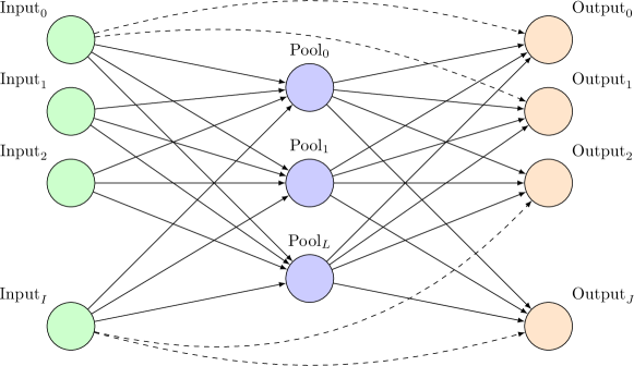
Figure 2: Pooling network $T=(N,A)$ with (i) input, (ii) pool, and (iii) output nodes. Straight arcs represent input-to-pool and pool-to-output flow. Dashed arcs illustrate bypass input-to-output flow.

4.3 Mathematical Models

This section provides the standard $P$- and $PQ$-formulations [24, 97, 163, 183] for modeling the pooling problem. For simplicity, these formulations are presented assuming the pooling network is complete, i.e. contains all possible arcs, but can be easily extended to arbitrary networks.

4.3.1 $P$-formulation

The $P$-formulation [97] uses the Section 4.2 arc flow and intermediate product attribute variables and can be stated using Equations (1). The resulting quadratic programming formulation includes bilinear terms due to linear blending.

$$\min_{\boldsymbol{x},\boldsymbol{y},\boldsymbol{z},\boldsymbol{p}} \sum_{(i,l)\in X}c_{i}x_{i,\,l}-\sum_{(l,j)\in Y}d_{j}y_{l,\,j}-\sum_{(i,j)\in Z}(d_{j}-c_{i})z_{i,\,j}$$ (1a)

$$A_{i}^{L}\leq\sum\limits_{l\in L}x_{i,\,l}+\sum_{j\in J}z_{i,\,j}\leq A_{i}^{U} i\in I$$ (1b)

$$\sum\limits_{j\in J}y_{l,\,j}\leq S_{l} l\in L$$ (1c)

$$D_{j}^{L}\leq\sum\limits_{l\in L}y_{l,\,j}+\sum_{i\in I}z_{i,\,j}\leq D_{j}^{U} j\in J$$ (1d)

$$\sum_{i\in I}x_{i,\,l}=\sum_{j\in J}y_{l,\,j} l\in L$$ (1e)

$$\sum_{i\in I}C_{i,\,k}x_{i,\,l}=p_{l,\,k}\sum_{j\in J}y_{l,\,j} l\in L,k\in K$$ (1f)

$$\sum_{l\in L}p_{l,\,k}y_{l,\,j}+\sum_{i\in I}C_{i,\,k}z_{i,\,j}\geq P_{j,\,k}^{L}(\sum_{l\in L}y_{l,\,j}+\sum_{i\in I}z_{i,\,j}) j\in J,k\in K$$ (1g)

$$\sum_{l\in L}p_{l,\,k}y_{l,\,j}+\sum_{i\in I}C_{i,\,k}z_{i,\,j}\leq P_{j,\,k}^{U}(\sum_{l\in l}y_{l,\,j}+\sum_{i\in I}z_{i,\,j}) j\in J,k\in K$$ (1h)

$$x_{i,\,l},y_{l,\,j},z_{i,\,j}\geq 0 i\in I,l\in L,j\in J$$ (1i)

$$p_{l,\,k}\geq 0 l\in L,k\in K$$ (1j)

Expression (1a) optimizes raw material costs and final product profits. Constraints (1b) - (1d) impose bounds on the raw material quantities, pool sizes, and final product quantities, respectively. Constraints (1e) ensure material balances. Constraints (1f) model linear blending. Constraints (1g) - (1h) enforce quality specifications. Constraints (1i) - (1j) ensure that all variables are non-negative.

4.3.2 $PQ$-formulation

The $PQ$-formulation [163, 183] extends the Ben-Tal et al. [24] pooling problem $Q$-formulation and replaces the $P$-formulation variables $x_{i,\,l}$ with path flow variables $v_{i,\,l,\,j}$ and proportion variables $q_{i,\,l}$, for $i\in I$, $l\in L$, and $j\in J$. Specifically, $v_{i,\,l,\,j}$ represents the flow transferred from input node $i\in i$ to output node $j\in J$ via pool node $l\in L$ and $q_{i,\,l}$ corresponds to the proportion of total flow entering pool $l\in L$ that originates from input node $i\in I$, i.e. $x_{i,\,l}=q_{i,\,l}\sum_{j\in J}y_{l,\,j}$ and $0\leq q_{i,\,l}\leq 1$. The $PQ$-formulation can be stated using Equations (2) and results in a tighter McCormick relaxation compared to the $P$-formulation. The $PQ$-relaxation can be strengthned by appending valid constraints derived with the reformulation linearization (RLT) technique [177].

$$\min_{\boldsymbol{y},\boldsymbol{z},\boldsymbol{v},\boldsymbol{q}} \sum_{(i,l,j)\in I\times L\times J}(c_{i}-d_{j})v_{i,\,l,\,j}+\sum\limits_{(i,j)\in Z}(c_{i}-d_{j})z_{i,\,j}$$ (2a)

$$A_{i}^{L}\leq\sum_{(l,j)\in Y}v_{i,\,l,\,j}+\sum\limits_{j\in J}z_{i,\,j}\leq A_{i}^{U} i\in I$$ (2b)

$$\sum_{(i,j)\in Z}v_{i,\,l,\,j}\leq S_{l} l\in L$$ (2c)

$$D_{j}^{L}\leq\sum_{(i,l)\in X}v_{i,\,l,\,j}+\sum_{i\in I}z_{i,\,j}\leq D_{j}^{U} j\in J$$ (2d)

$$v_{i,\,l,\,j}=q_{i,\,l}y_{l,\,j} i\in I,j\in J,l\in L$$ (2e)

$$\sum_{i\in I}q_{i,\,l}=1 l\in L$$ (2f)

$$\sum_{i\in I}v_{i,\,l,\,j}=y_{l,\,j} l\in L,j\in Y$$ (2g)

$$\sum_{(i,l)\in X}(C_{i,\,k}-P_{j,\,k}^{L})v_{i,\,l,\,j}+\sum_{i\in I}(C_{i,\,k}-P_{j,\,k}^{L})z_{i,\,j}\geq 0 j\in J$$ (2h)

$$\sum_{(i,l)\in X}(C_{i,\,k}-P_{j,\,k}^{U})v_{i,\,l,\,j}+\sum_{i\in I}(C_{i,\,k}-P_{j,\,k}^{U})z_{i,\,j}\leq 0 j\in J$$ (2i)

$$y_{l,\,j},z_{i,\,j}\geq 0 i\in I,l\in L,j\in J$$ (2j)

$$0\leq q_{i,\,l}\leq 1 i\in I,l\in L$$ (2k)

Expression (2a) minimizes the total cost. Constraints (2b) - (2d) enforce bounds on the raw material quantities, pool sizes, and final product quantities, respectively. Constraints (2e) - (2g) express material balances. Constraints (2h) - (2i) impose quality specifications. Constraints (2j) - (2k) ensure non-negativity of flow variables and fraction bounds.

4.4 Computational Complexity and Approximation Algorithms

This section discusses the known computational complexity and approximation algorithms for the pooling problem. Table 1 additionally summarizes the computational complexity results discussed in this section.

When there are no quality constraints, i.e. $|K|=0$, or $P_{j,k}^{L}=0$ and $P_{j,k}^{U}=+\infty$ for each $j\in J$ and $k\in K$, pooling becomes an instance of the well-known minimum cost flow problem which is polynomially solvable. Pooling is also a tractable LP when there are no intermediate pools and the problem is referred to as blending. In the more general case with both quality constraints and intermediate pools, Table 1 reports state-of-the-art computational complexity results for subproblems with (i) set cardinality restrictions, (ii) special network structure and (iii) supply/demand/capacity restrictions.

Alfaki and Haugland [9] show that pooling is strongly $\mathcal{NP}$-hard even in the special case with a single pool, i.e. $|L|=1$, through a reduction from the independent set problem. The problem remains $\mathcal{NP}$-hard for instances with a single quality attribute, i.e. $|K|=1$, via a reduction from Exact Cover by 3-Sets [31]. On the other hand, in the singleton cases with a single input or output, i.e. $\min\{|I|,|J|\}=1$, pooling can be easily formulated as an LP and is therefore polynomially solvable [53]. These findings have motivated further investigations on pooling with set cardinality restrictions. For instances with a single pool with no input-output arcs where the number of inputs [31], outputs [9], or attributes [9, 94] is bounded by a constant, i.e. $\min\{|I|,|J|,|K|\}=O(1)$, the problem can be solved in polynomial time using a series of LPs. In the case $|K|=1$ with a single quality attribute where there are either two inputs, or two outputs, i.e. $\min\{|I|,|J|\}=2$, the problem is still $\mathcal{NP}$-hard by a reduction from Exact Cover by 3-Sets. Finally, when $|I|=|J|=2$, pooling is known to be weakly $\mathcal{NP}$-hard through a reduction from Partition.

Haugland [95] shows that pooling is $\mathcal{NP}$-hard for problem instances with sparse network structure. Let $\Delta_{i}^{\text{out}}$ and $\Delta_{l}^{\text{out}}$ be the out-degree, i.e. number of outgoing arcs, of input $i\in I$ and pool $l\in L$, respectively. When every out-degree is at most two, i.e. $\max\{\Delta_{i}^{\text{out}},\Delta_{l}^{\text{out}}\}\leq 2$, Haugland [95] presents an $\mathcal{NP}$-hardness reduction from maximum satisfiability. Denote by $\Delta_{l}^{\text{in}}$ and $\Delta_{j}^{\text{in}}$ the in-degree, i.e. number of ingoing arcs, of pool $l\in L$ and output $j\in J$, respectively. When each in-degree does not exceed two, i.e. $\max\{\Delta_{l}^{\text{in}},\Delta_{j}^{\text{in}}\}\leq 2$, pooling is $\mathcal{NP}$-hard through a reduction from minimum satisfiability [95]. However, in the case where each pool has either in-degree or out-degree equal to one, i.e. $\min\{\Delta_{l}^{\text{out}},\Delta_{l}^{\text{in}}\}=1$, the problem is polynomially solvable [53, 96]. Finally, for instances with a single pool and attribute, unlimited supplies/pool capacities and fixed demands, the pooling problem is strongly-polynomially solvable [17].

Table 1: Pooling Problem Computational Complexity Results

Subproblem	Complexity	Reduction
Singleton subproblems
$|I|=1$	$\mathcal{P}$	-
$|J|=1$	$\mathcal{P}$	-
$|L|=1,\ Z=\emptyset$	$\mathcal{NP}$-hard	Independent Set
$|K|=1$	$\mathcal{NP}$-hard	Exact Cover by 3-Sets
Other cardinality-restricted special cases
$|L|=1,\ |I|=O(1),\ Z=\emptyset$	$\mathcal{P}$	-
$|L|=1,\ |J|=O(1),\ Z=\emptyset$	$\mathcal{P}$	-
$|L|=1,\ |K|=O(1),\ Z=\emptyset$	$\mathcal{P}$	-
$|I|=2,\ |K|=1$	$\mathcal{NP}$-hard	Exact Cover by 3-Sets
$|J|=2,\ |K|=1$	$\mathcal{NP}$-hard	Exact Cover by 3-Sets
$|I|=2,\ |J|=2,\ |K|=1$	$\mathcal{NP}$-hard	Partition
Special network structure
$\min\{\Delta_{l}^{\text{out}},\ \Delta_{l}^{\text{in}}\}=1$	$\mathcal{P}$	-
$\Delta_{i}^{\text{out}}\leq 2,\ \Delta_{l}^{\text{out}}\leq 2$	$\mathcal{NP}$-hard	Maximum Satisfiability
$\Delta_{l}^{\text{in}}\leq 2,\ \Delta_{j}^{\text{in}}\leq 2$	$\mathcal{NP}$-hard	Minimum Satisfiability
Supply, demand, and pool capacity restrictions
$|L|=1,\ |K|=1,\ A^{L}_{i}=0,A^{U}_{i}=\infty,\ S_{l}=\infty,\ D^{L}_{j}=D^{U}_{j}$	$\mathcal{P}$	-

The only known theoretical performance bounds for pooling are an $O(n)$-approximation algorithm and an $\Omega(n^{1-\epsilon})$ inapproximability result, for $\epsilon>0$, by Dey and Gupte [53]. The proposed algorithm solves the relaxation obtained by applying piecewise linear McCormick envelopes to the bilinear terms of the $PQ$-formulation [89, 90]. Overestimators and underestimators are computed by partitioning the domain of proportion variables to a finite MILP-representable set. For the negative result, Dey and Gupte [53] present an approximation-preserving reduction from independent set.

5 Process Scheduling

Scheduling process operations, a.k.a. batch scheduling, is crucial in different application areas including chemical manufacturing, pharmaceutical production [114], food industry [181], and oil refining [92]. Process scheduling problems are the topic of many fruitful investigations in the PSE literature [38, 64, 92, 143, 194]. The goal is to efficiently allocate the limited resources, e.g. processing units, of manufacturing plants to tasks and decide the product batch sizes so as to construct multiple intermediate and final products satisfying the customer demand. These products are often based on recipes in the form of state-task networks where each task receives raw materials and intermediate products to generate new products [109, 174]. State-task networks may model general batch processes including material mixing, splitting, recycling, as well as different storage policies [106]. Fig. 3 presents an example of a state-task network. Typically, process scheduling involves solving $\mathcal{NP}$-hard, mixed-integer linear programming problems which require algorithms exploiting the state-task network’s structure.

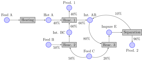
Figure 3: Network structure for the state-task network by Kondili et al.[109]

5.1 Brief Literature Overview

Scheduling is a relatively recent area in PSE [140, 164] and has received considerable attention after the seminal work by Kondili et al. [109] who introduced the state-task network framework for modeling mixing and splitting of material batches. Pantelides [153] extended the state-task network to the notion of a Resource-Task Network (RTN) for incorporating multiple resources in a unified setting. Process scheduling problems include a variety of aspects that need to be considered, such as different production stages, storage policies, demand patterns, changeovers, resource constraints, time constraints, and uncertainty. Furthermore, they require optimizing different objective functions, e.g. makespan, production costs, or sales profit. There is significant work providing surveys and problem classification for process scheduling [38, 64, 92, 125, 134, 143].

Significant literature solves process scheduling problems using MILP, this work is supported by the significant progress in CPU speed and algorithms in the last two decades. State-of-the-art mathematical modeling develops discrete-time and continuous-time formulations [136, 135]. These approaches are strengthened by reformulation and tightening methods [100, 169, 182, 189]. Branch-and-cut, decomposition, constraint programming, metaheuristic, hybrid approaches, and satisfiability modulo theories are also explored [37, 111, 137, 149, 185, 188, 197]. Recently, generalized-disjunctive programming has emerged as a novel framework for effectively solving process scheduling problems using big-M and convex hull reformulations [36]. In addition, rescheduling has been used as a tool for mitigating the effect of disturbances under uncertainty [88, 87].

5.2 Problem Definition

A process scheduling problem instance consists of a state-task network specifying a recipe for generating chemical products from raw materials. Formally, a state-task network is a directed bipartite graph $N=(S\cup I,A)$ with a partition of nodes into a subset $S$ corresponding to states, i.e. raw materials, intermediate, and final products, and a subset $I$ representing tasks. The network $N$ is bipartite, i.e. the set $A=A^{-}\cup A^{+}$ of arcs consists of consumption arcs $A^{-}\subseteq S\times I$ and production arcs $A^{+}\subseteq I\times S$. Arc $(s,i)\in A^{-}$ implies that task $i\in I$ consumes a positive amount of state $s\in S$. Analogously, arc $(i,s)\in A^{+}$ indicates that task $i\in I$ produces a positive amount of state $s\in S$. There is a set $J$ of processing units for executing tasks. Each unit may process at most one task per unit of time. Denote by $J_{i}\subseteq J$ the subset of units that may perform task $i\in I$ and by $I_{j}=\{i:(j\in J_{i})\wedge(i\in I)\}$ the set of tasks that may be performed by unit $j\in J$. Moreover, let $\ell$ be the time horizon length and $T=[0,\ell]$. If task $i\in I$ begins execution on unit $j\in J_{i}$ at time $t\in T$, then it may process a variable amount $b_{i,j,t}$ of material, a.k.a. batch size, for $p_{i,j}$ units of time, and completes at time $t+p_{i,j}$. Let $b_{i,j}^{L}$ and $b_{i,j}^{U}$ be the minimum and maximum capacity, respectively, of unit $j\in J$ when processing task $i\in I$. Continuous variable $b_{i,j,t}$ is allowed to take any value in the interval $[b_{i,j}^{L},b_{i,j}^{U}]$. Denote by $f_{i,s}^{-}$ and $f_{i,s}^{+}$ the material fraction entering and exiting processing, respectively, as state $s\in S$ when task $i\in I$ is processed. If $S_{i}^{-}=\{s:((s,i)\in A^{-})\wedge(s\in S)\}$ and $S_{i}^{+}=\{s:((i,s)\in A^{+})\wedge(s\in S)\}$ are the consumables and products of task $i\in I$, respectively, then task $i$ consumes $f_{i,s}^{-}b_{i,j,t}$ portion of state $s\in S_{i}^{-}$ and produces $f_{i,s}^{+}b_{i,j,t}$ quantity of state $s\in S_{i}^{+}$. Suppose that $I_{s}^{+}=\{i:((i,s)\in A^{+})\wedge(i\in I)\}$ and $I_{s}^{-}=\{i:((s,i)\in A^{-})\wedge(i\in I)\}$ are the sets of tasks producing and consuming, respectively, state $s\in S$. Then, $\sum_{i\in I_{s}^{+}}\sum_{j\in J_{i}}\sum_{t\in T}f_{i,s}^{+}b_{i,j,t-p_{i,j}}$ amount is produced and $\sum_{i\in I_{s}^{-}}\sum_{j\in J_{i}}\sum_{t\in T}f_{i,s}^{-}b_{i,j,t}$ quantity is consumed for state $s\in S$ at $t\in T$. A.2 presents the notation for process scheduling.

The goal of process scheduling is to satisfy a demand $d_{s}$ for each state $s\in S$. Denote by $y_{s,t}$ the amount of $s\in S$ at time slot $t\in T$. Without loss of generality, we assume that $y_{s,0}=0$, i.e. there is initially zero amount of state $s\in S$. When the time horizon completes, the obtained solution must satisfy $y_{s,\ell}\geq d_{s}$ for each $s\in S$. The objective is to schedule the tasks on the units and decide the batch sizes so that the makespan $z$, i.e. the time at which the last task completes, is minimized.

5.3 Mathematical Models

The main approaches for formulating process scheduling problems as MILP problems are typically classified as (i) discrete-time [109, 174], or (ii) continuous-time [136]. Floudas and Lin [64] and Méndez et al. [143] provide thorough discussions on the advantages of each. Discrete-time formulations partition time into a large number of time intervals. Continuous-time formulations (i) use a small number of event points resulting in fewer variables, and (ii) express inventory and backlog costs linearly. However, continuous-time formulations generally tend to be nonlinear. Mixed-time representations utilize both the discrete-time and continuous-time models [116, 133].

5.3.1 Discrete-Time Formulation

Discrete-time formulations partition the time horizon into a set $T=\{1,\ldots,\ell\}$ of equal-length slots. Integer variable $x_{i,j,t}$ indicates whether task $i\in I$ is executed by unit $j\in J$ starting at time $t\in T$. Continuous variable $b_{i,j,t}$ specifies the corresponding batch size. Continuous variables $y_{s,t}$ denote the stored amount of state $s\in S$ at time $t\in T$. Finally, continuous variable $z$ computes the makespan. Process scheduling can be modeled using the Eq. (3) MILP formulation.

$$\min\quad z$$ (3a)

$$z\geq x_{i,j,t}(t+p_{i,j}) i\in I,j\in J_{i},t\in T$$ (3b)

$$\sum_{i\in I_{j}}\sum_{t^{\prime}=t-p_{i,j}+1}^{t}x_{i,j,t^{\prime}}\leq 1 j\in J,t\in T$$ (3c)

$$x_{i,j,t}b_{i,j}^{L}\leq b_{i,j,t}\leq x_{i,j,t}b_{i,j}^{U} i\in I,j\in J_{i},t\in T$$ (3d)

$$y_{s,t}=y_{s,t-1}+\sum_{i\in I^{+}_{s}}\sum_{j\in J_{i}}f_{i,s}^{+}b_{i,j,t-p_{i,j}+1}-\sum_{i\in I_{s}^{-}}\sum_{j\in J_{i}}f_{i,s}^{-}b_{i,j,t} s\in S,t\in T$$ (3e)

$$y_{s,\ell}\geq d_{s},y_{s,1}=0 s\in S$$ (3f)

$$x_{i,j,t}\in\{0,1\} i\in I,j\in J_{i},t\in T$$ (3g)

$$z,b_{i,j,t},y_{s,t}\geq 0 i\in I,j\in J_{i},s\in S,t\in T$$ (3h)

Expression (3a) minimizes makespan. Constraints (3b) define the makespan. Constraints (3c) ensure that each unit processes at most one task at each point in time. Constraints (3d) and (3e) express unit capacities and material conservation, respectively. Constraints (3f) enforce that the demand is statisfied. Finally, constraints (3g) - (3h) impose that integer and continuous variables are binary and non-negative, respectively.

5.3.2 Continuous-Time Formulation

Continuous-time formulations divide the time horizon into a set of slots, similarly to discrete-time formulations. The number of slots is fixed, but the slots are not necessarily of equal length. The slot boundaries are determined by a set $T$ of $\ell$ variable time points. Continuous variable $t_{k}$ specifies the rightmost time point $k\in T$ of one slot and the leftmost time point of the subsequent slot. Furthermore, each job’s starting and completion time is mapped to a time point. Binary variables $x_{i,k}^{S}$ and $x_{i,k}^{F}$ express whether task $i\in I$ begins and completes, respectively, at time point $k\in T$. To match time points with task starting and completion times, continuous variables $t_{i,k}^{S}$ and $t_{i,k}^{F}$ compute the start and finish time of task $i\in I$ beginning at time point $k\in T$. Continuous variables $p_{i,k}$ and $b_{i,k}$ correspond to the processing time and batch size of task $i\in I$ starting at time point $k\in T$. Finally, continuous variable $y_{s,k}$ models the amount of state $s\in S$ at time point $k\in T$. Without loss of generality, we assume that $|J_{i}|=1$ for each $i\in I$, i.e. tasks $i$ can only be executed by a single unit. To model the case $|J_{i}|>1$, we may add multiple occurrences of the same task. Furthermore, we note that continuous-time formulations may easily incorporate variable task durations. Specifically, we suppose that task $i\in I$ has a variable duration $\alpha_{i}$ that depends on the batch size, in addition to a fixed duration $\beta_{i}$. Then, variable $p_{i,k}$ denotes the processing time of job $i\in I$ starting at time point $k\in T$.

$$\min\quad z$$ (4a)

$$z\geq t_{i,k}^{S}+p_{i,k} i\in I,k\in T$$ (4b)

$$p_{i,k}=\alpha_{i}x_{i,k}^{S}+\beta_{i}b_{i,k}^{S} i\in I,k\in T$$ (4c)

$$t_{i,k}^{S}\leq t_{k}+H(1-x_{i,k}^{S}) i\in I,k\in T$$ (4d)

$$t_{i,k}^{S}\geq t_{k}-H(1-x_{i,k}^{S}) i\in I,k\in T$$ (4e)

$$t_{i,k}^{F}\leq t_{k}+p_{i,k}+H(1-x_{i,k}^{S}) i\in I,k\in T$$ (4f)

$$t_{i,k}^{F}\geq t_{k}+p_{i,k}-H(1-x_{i,k}^{S}) i\in I,k\in T$$ (4g)

$$t_{i,k}^{F}-t_{i,k-1}^{F}\leq Hx_{i,k}^{S} i\in I,k\in T\setminus\{1\}$$ (4h)

$$t_{i,k-1}^{F}\leq t_{k}+H(1-x_{i,k}^{F}) i\in I,k\in T\setminus\{1\}$$ (4i)

$$t_{i,k-1}^{F}\geq t_{k}-H(1-x_{i,k}^{F}) i\in I,k\in T\setminus\{1\}$$ (4j)

$$t_{1}=0,t_{k-1}\leq t_{k},t_{\ell}=H k\in T\setminus\{1\}$$ (4k)

$$\sum_{i\in I_{j}}\sum_{k^{\prime}\leq k}(x_{i,k^{\prime}}^{S}-x_{i,k}^{F})\leq 1 j\in J,k\in T$$ (4l)

$$\sum_{k\in T}x_{i,k}^{S}=\sum_{k\in T}x_{i,k}^{F} i\in I$$ (4m)

$$x_{i,k}^{S}b_{i}^{L}\leq b_{i,k}\leq x_{i,k}^{S}b_{i}^{U} i\in I,k\in T$$ (4n)

$$y_{s,k}=y_{s,k-1}+\sum_{i\in I_{s}^{+}}f_{i,s}^{+}b_{i,k-1}-\sum_{i\in I_{s}^{-}}f_{i,s}^{-}b_{i,k} s\in S,k\in T\setminus\{1\}$$ (4o)

$$y_{s,\ell}\geq d_{s} s\in S,k\in T$$ (4p)

$$x_{i,k}^{S},x_{i,k}^{F}\in\{0,1\} i\in I,k\in T$$ (4q)

$$t_{k},t_{i,k}^{S},t_{i,k}^{F},p_{i,k},b_{i,k},y_{s}\geq 0 i\in I,k\in T,s\in S$$ (4r)

Expression (4a) minimizes makespan. Constraints (4b) are the makespan definition. Constraints (4c) calculate the job processing time. Binary activation constraints (4d) - (4j) map continuous time variables to time points. Constraints (4k) impose time horizon boundaries and the non-decreasing order of time points. Constraints (4l) enforce that each unit processes at most one task per time. Constraints (4m) ensure that every task that begins processing must also complete. Constraints (4n) incorporate unit capacities. Constraints (4o) express mass balance. Constraints (4p) model storage capacities. Finally, constraints (4q) - (4r) ensure that continuous and integer variables are non-negative and binary, respectively.

5.4 Computational Complexity and Approximation Algorithms

Process scheduling problems are frequently characterized as computationally challenging [64, 92]. However, computational complexity investigations are limited and isolated. To our knowledge, Burkard et al. [34] have only work in this direction. Burkard et al. [34] observe that process scheduling (i) is strongly $\mathcal{NP}$-hard as a generalization of the job shop scheduling problem, and (ii) remains $\mathcal{NP}$-hard even in the special case with two states through a straightforward reduction from knapsack. Heuristics have been reported as a tool for solving large-scale process scheduling instances [92, 143, 154]. Nevertheless, only few early works in the area develop heuristics exploiting the problem’s combinatorial structure, e.g. greedy layered [30] and discrete-time relaxation rounding [34]. Furthermore, there is lack of analytically proven performance guarantees.

The above observations are opposed to the tremendous contributions of computational complexity and approximation algorithms in scheduling theory. A classical scheduling problem may be defined using the three-field notation which incorporates [82]: (i) a machine environment, (ii) job characteristics, and (iii) an objective function. The goal is to decide when and where to execute the jobs, i.e. at which times and on which machines, so that the objective function is optimized. Single stage machine environments include: identical, related, and unrelated machines. Multistage machine environments can be: open shops, flow shops, or job shops. Examples of job characteristics are: release times, deadlines, and precedence constraints. Objective functions include: makespan, response time, tardiness, throughput and others. Despite the commonalities between process scheduling and classical scheduling theory, there is a striking absence of connections between the two fields. Their synergy constitutes a particularly interesting future direction and has strong potential for successfully solving open process scheduling problems. To this end, Chen et al. [42] and The Scheduling Zoo [184] provide an extensive survey of results for fundamental scheduling problems. Brucker [33], Leung [122] and Pinedo [159] present a collection of algorithms and techniques for effectively solving such problems.

6 Heat Exchanger Network Synthesis

Heat exchanger network synthesis is one of the most extensively studied problems in chemical engineering [28, 57, 68, 85, 180]. Major heat exchanger network synthesis applications include energy systems producing liquid transportation fuels [62, 152], natural gas refineries [15, 59], refrigeration systems [175], batch processes [35, 200], and water utilization systems [13]. Heat exchanger network synthesis minimizes the total investment and operating costs in chemical processes. In particular, heat exchanger network synthesis: (i) improves energy efficiency by reducing heating utility usage, (ii) optimizes network costs by accounting for the number of heat exchanger units and area physical constraints, and (iii) improves energy recovery by integrating hot and cold process streams [56, 63]. The goal is designing a heat exchanger network matching hot streams to cold streams and recycling residual heat, by taking into account the nonlinear nature of heat exchange and thermodynamic constraints. Heat exchanger network synthesis is an $\mathcal{NP}$-hard, MINLP instance with (i) nonconvex nonlinearities for enforcing energy balances, and (ii) discrete decisions for placing heat exchanger units. This section investigates the nonlinear and integer heat exchanger network synthesis parts individually by considering the multistage minimum utility cost, and minimum number of matches problems separately.

6.1 Brief Literature Overview

Optimization methods for heat exchanger network synthesis can be classified as: (i) simultaneous, or (ii) sequential. Simultaneous methods produce globally optimal solutions. Sequential methods do not provide any guarantee of optimality, but are useful in practice. Simultaneous methods formulate heat exchanger network synthesis as a single MINLP, e.g. Papalexandri and Pistikopoulos [156]. Ciric and Floudas [45] propose the hyperstructure MINLP formulating heat exchanger network synthesis without decomposition based on the stream superstructure introduced by Floudas et al. [61]. Yee and Grossmann [199] develop the multistage MINLP (a.k.a. SYNHEAT model) using a stagewise superstructure. Because the multistage MINLP assumes isothermal mixing at each stage, the nonlinear heat balances are simplified and performed only between stages. Sequential methods decompose heat exchanger network synthesis into three distinct subproblems: (i) minimum utility cost, (ii) minimum number of matches, and (iii) minimum investment cost. These subproblems are more tractable than simultaneous heat exchanger network synthesis. In particular, Cerda and Westerburg [41], Cerda et al. [40], Papoulias and Grossmann [157] suggest the transportation and transshipment models formulating the minimum utility cost problem as LP and the minimum number of matches problem as MILP. Floudas et al. [61] propose the stream superstructure formulating the minimum investment cost problem as an NLP. Other heat exchanger network synthesis approaches exploit the problem’s thermodynamic nature, and mathematical and physical insights in order to design more efficient algorithms. [2, 3, 84, 86, 112, 119, 127, 128, 129, 139, 150, 158, 162].

6.2 Problem Definitions

A heat exchanger network synthesis instance consists of a set $H$ of hot streams to be cooled down and a set $C$ of cold streams to be heated up. Each hot stream $i\in H$ and cold stream $j\in C$ is associated with an initial, inlet temperature $T_{i}^{\text{in}}$, $T_{j}^{\text{in}}$, target, outlet temperature $T_{i}^{\text{out}}$, $T_{j}^{\text{out}}$, and flow rate heat capacity $F_{i}$, $F_{j}$, respectively. The temperature of hot stream $i\in H$ must be decreased from $T_{i}^{\text{in}}$ down to $T_{i}^{\text{out}}$, while the temperature of cold stream $j\in C$ has to be increased from $T_{j}^{\text{in}}$ up to $T_{j}^{\text{out}}$. For each $i\in H$ and $j\in C$, flow rate heat capacities $F_{i}$ and $F_{j}$ specify the quantity of heat that a stream releases and absorbs, respectively, per unit of temperature change. That is, hot stream $i\in H$ supplies $F_{i}(T_{i}^{\text{in}}-T_{i}^{\text{out}})$ units of heat, while cold stream $j\in C$ demands $F_{j}(T_{j}^{\text{out}}-T_{j}^{\text{out}})$ units of heat. A.3 presents the notation for heat exchanger network synthesis.

6.2.1 Multistage Minimum Utility Cost

In multistage heat exchanger network synthesis, heat transfers between streams occur in a set $S$ of $\ell$ different stages. Hot streams flow from the stage $1$ to stage $\ell$, while cold streams flow, in the opposite direction, from stage $\ell$ to stage $1$. When a hot, respectively cold, stream enters stage $k\in S$, it is split into substreams each one exchanging heat with exactly one cold, respectively hot, stream and these substreams are merged back together when the stream exits the stage. Figure 4 illustrates splitting and mixing. For $k\in S$, denote by $t_{i,k}$ the temperature of hot stream $i\in H$ when exiting and entering the stages $k$ and $k+1$, respectively. Similarly, let $t_{j,k}$ be the initial and last temperature of cold stream $j\in H$ at stages $k$ and $k+1$, respectively, for $k\in S$. The multistage minimum utility cost problem decides how to split the streams in each stage. The substream of $i\in H$ exchanging heat with $j\in C$ at stage $k\in S$ gets flow rate heat capacity $f_{i,j,k}^{H}$. Similarly, the substream of $j\in C$ exchanging heat with $i\in H$ at stage $k\in S$ is assigned flow rate heat capacity $f_{i,j,k}^{C}$. It must be the case that $\sum_{j\in C}f_{i,j,k}^{H}=F_{i}$ and $\sum_{i\in H}f_{i,j,k}^{C}=F_{j}$, for all $k\in S$. If $i\in H$ is matched with $j\in C$ at $k\in S$, the corresponding substream of $i$ and $j$ results with a temperature $t_{i,j,k}^{H}$ and $t_{i,j,k}^{C}$, respectively, when the stage completes. At stage $k\in S$, hot stream $i\in H$ and cold stream $j\in C$ have final temperatures $t_{i,k}$ and $t_{j,k-1}$ such that $F_{i}t_{i,k}=\sum_{j\in C}f_{i,j,k}^{H}t_{i,j,k}^{H}$ and $F_{j}t_{j,k-1}=\sum_{i\in H}f_{i,j,k}^{C}t_{i,j,k}^{C}$. The total heat exchanged between $i$ and $j$ at $k$ is $q_{i,j,k}=f_{i,j,k}^{H}(t_{i,k}-t_{i,j,k}^{H})$ and $q_{i,j,k}=f_{i,j,k}^{C}(t_{i,j,k}^{C}-t_{j,k})$, i.e. there is heat conservation. A hot and cold utility may provide or extract heat at unitary costs $c^{HU}$ and $c^{CU}$. The cold utility exports $Q_{i}^{CU}=F_{i}(t_{i,\ell}-T_{i}^{\text{out}})$ units of heat from hot stream $i\in H$. Analogously, the hot utility supplies $Q_{j}^{HU}=F_{j}(T_{j}^{\text{out}}-t_{j,0})$ units of heat to cold stream $j\in C$. The goal is to exchange heat and reach the target temperature for each stream so that the total utility cost $\sum_{i\in H}c^{CU}Q_{i}^{CU}+\sum_{j\in C}c^{HU}Q_{j}^{HU}$ is minimized.

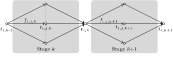
Figure 4: Illustration of multistage heat exchanger network synthesis. Hot stream $i\in H$ across multiple stages in increasing order of their indices. At stage $k\in S$, stream $i$ is split into substreams.

6.2.2 Minimum Number of Matches Problem

In the minimum number of matches problem, heat transfers occur similarly to standard network flow problems [4]. A problem instance only consists of streams. The utilities are considered as streams whose parameters, i.e. flow rate heat capacities, inlet and outlet temperatures, are computed by solving a minimum utility cost LP to ensure heat conservation. Specifically, hot stream $i\in H$ exports $h_{i}=F_{i}(T_{i}^{\text{in}}-T_{i}^{\text{out}})$ units of heat, cold stream $j\in C$ receives $c_{j}=F_{j}(T_{j}^{\text{out}}-T_{j}^{\text{in}})$ units of heat, and $\sum_{i\in H}h_{i}=\sum_{j\in C}c_{j}$. A minimum heat approach temperature $\Delta T_{\min}$ accounts for the energy lost by the system. We may assume that $\Delta T_{\min}=0$, because any problem instance can be transformed to an equivalent one satisfying this assumption. Let $T_{0}>T_{1}>\dots>T_{r}$ be all discrete inlet and outlet temperature values. The temperature range is partitioned into a set $T=\{[T_{t},T_{t-1}]:1\leq t\leq r\}$ of consecutive temperature intervals. In temperature interval $t\in T$, hot stream $i\in H$ exports $\sigma_{i,t}=F_{i}(T_{t-1}-T_{t})$ units if $[T_{t},T_{t-1}]\subseteq[T_{i}^{\text{out}},T_{i}^{\text{in}}]$, and $\sigma_{i,t}=0$ otherwise. Likewise, cold stream $j\in C$ receives $\delta_{j,t}=F_{j}(T_{t-1}-T_{t})$ units of heat if $[T_{t},T_{t-1}]\subseteq[T_{j}^{\text{in}},T_{j}^{\text{out}}]$, and $\delta_{j,t}=0$ otherwise. A feasible solution specifies a way to transfer the hot streams’ heat supply to the cold streams, i.e. an amount $q_{i,s,j,t}$ of heat exchanged between hot stream $i\in H$ in temperature interval $s\in T$ and cold stream $j\in C$ in temperature interval $t\in T$. Heat may only flow to the same or a lower temperature interval, i.e. $q_{i,s,j,t}=0$, for each $i\in H$, $j\in C$ and $s,t\in T$ such that $s>t$. A hot stream $i\in H$ and a cold stream $j\in C$ are matched, if there is a positive amount of heat exchanged between them, i.e. $\sum_{s,t\in T}q_{i,s,j,t}>0$. The objective is to find a feasible solution minimizing the number of matches $(i,j)$.

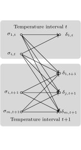
(a) Transportation Model

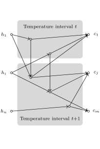
(b) Transshipment Model

Figure 5: In the transportation model [41], each hot stream $i$ supplies $\sigma_{i,t}$ units of heat in temperature interval $t$ which can be received, in the same or a lower temperature interval, by a cold stream $j$ which demands $\delta_{j,t}$ units of heat in $t$. In the transshipment model [157], there are also intermediate nodes transferring residual heat to a lower temperature interval. This figure is adapted from Furman and Sahinidis [69].

6.3 Mathematical Models

This section presents a quadratic programming (QP) formulation for the multistage minimum utility cost problem and an MILP formulation for the minimum number of matches problem.

6.3.1 Multistage Minimum Utility Cost Problem

In the Eq. (5) QP formulation, continuous variables $Q_{i}^{CU}$ and $Q_{j}^{HU}$ compute the heat transferred from hot stream $i\in H$ to the cold utility and from the hot utility to cold stream $j\in C$. Continuous variables $t_{i,k}$ and $t_{j,k}$ correspond to the temperature of hot stream $i\in H$ and cold stream $j\in C$ when exiting and entering stage $k\in S$, respectively. Continuous variables $t_{i,j,k}^{H}$ and $t_{i,j,k}^{C}$ express the exiting temperature of hot stream $i\in H$ and cold stream $j\in C$ in heat exchanger $(i,j,k)$, respectively. Continuous variables $f_{i,j,k}^{H},f_{i,j,k}^{C}$ model the flow rate heat capacity of the hot and cold substream in heat exchanger $(i,j,k)$. Auxiliary continuous variables $q_{i,j,k}$ are the heat exchanged via heat exchanger $(i,j,k)$.

$$\min\quad \sum_{i\in H}c^{CU}Q_{i}^{CU}+\sum_{j\in C}c^{HU}Q_{j}^{HU}$$ (5a)

$$Q_{i}^{CU}=F_{i}(t_{i,\ell}-T_{i}^{\text{out}}) i\in H$$ (5b)

$$Q_{j}^{HU}=F_{j}(T_{j}^{\text{out}}-t_{j,0}) j\in C$$ (5c)

$$\sum_{j\in C}f_{i,j,k}^{H}=F_{i}^{H} i\in H,k\in S$$ (5d)

$$\sum_{i\in H}f_{i,j,k}^{C}=F_{j}^{C} j\in C,k\in S$$ (5e)

$$q_{i,j,k}=f_{i,j,k}^{H}(t_{i,k-1}-t_{i,j,k}^{H}) i\in H,j\in C,k\in S$$ (5f)

$$q_{i,j,k}=f_{i,j,k}^{C}(t_{i,j,k}^{C}-t_{j,k}) i\in H,j\in C,k\in S$$ (5g)

$$F_{i}t_{i,k}=\sum_{j\in C}f_{i,j,k}^{H}t_{i,j,k}^{H} i\in H,k\in S$$ (5h)

$$F_{j}t_{j,k-1}=\sum_{i\in H}f_{i,j,k}^{C}t_{i,j,k}^{C} j\in C,k\in S$$ (5i)

$$t_{i,k-1}\leq t_{i,k} i\in H,k\in S$$ (5j)

$$t_{j,k-1}\leq t_{j,k} j\in C,k\in S$$ (5k)

$$T_{i}^{\text{in}}=t_{i,0}\geq t_{i,\ell}\geq T_{i}^{\text{out}} i\in H$$ (5l)

$$T_{j}^{\text{out}}\geq t_{j,0}\geq t_{j,\ell}=T_{j}^{\text{in}} j\in H$$ (5m)

$$t_{i,k},t_{j,k},t_{i,j,k}^{H},t_{i,j,k}^{C}\geq 0 i\in H,j\in C,k\in S$$ (5n)

$$f_{i,j,k}^{H},f_{i,j,k}^{C},q_{i,j,k},Q_{i}^{CU},Q_{j}^{HU}\geq 0 i\in H,j\in C,k\in S$$ (5o)

Expression (5a) minimizes the total heating utility cost. Constraints (5b) and (5c) compute the heat absorbed by cold utilities and the heat supplied by hot utilities. Constraints (5d) and (5e) divide the flow rate heat capacity of each stream fractionally to its corresponding substreams. Constraints (5f) and (5g) compute the heat load exchanged between each pair of streams and enforce heat conservation. Constraints (5h) and (5i) compute temperature of each stream by mixing substreams. Constraints (5j) and (5k) enforce temperature monotonicity. Constraints (5l) and (5m) assign initial temperature values and impose final temperature bounds. Finally, Constraints (5n) and (5o) ensure that all variables are non-negative.

6.3.2 Minimum Number of Matches Problem

The minimum number of matches can be formulated as an MILP using either the transportation, or the transshipment model in Figure 5. The former model represents heat as a commodity transported from supply nodes to destination nodes. For each hot stream $i\in H$, there is a set of supply nodes, one for each temperature interval $s\in T$ with $\sigma_{i,s}>0$. For each cold stream $j\in C$, there is a set of demand nodes, one for each temperature interval $t\in T$ with $\delta_{j,t}>0$. There is an arc between the supply node $(i,s)$ and the destination node $(j,t)$ if $s\leq t$, for each $i\in H$, $j\in C$ and $s,t\in T$. Continuous variable $q_{i,s,j,t}$ specifies the heat transferred from hot stream $i\in H$ in temperature interval $s\in T$ to cold stream $j\in C$ in temperature interval $t\in T$. Binary variable $y_{i,j}$ indicates whether streams $i\in H$ and $j\in C$ are matched. Big-M parameter $U_{i,j}$ bounds the amount of heat exchanged between every pair of hot stream $i\in H$ and cold stream $j\in C$, e.g. $U_{i,j}=\min\{h_{i},c_{j}\}$. Then, the problem can be modeled with formulation (6).

min $$\sum_{i\in H}\sum_{j\in C}y_{i,j}$$ (6a)

$$\sum_{j\in C}\sum_{t\in T}q_{i,s,j,t}=\sigma_{i,s} i\in H,s\in T$$ (6b)

$$\sum_{i\in H}\sum_{s\in T}q_{i,s,j,t}=\delta_{j,t} j\in C,t\in T$$ (6c)

$$\sum_{s,t\in T}q_{i,s,j,t}\leq U_{i,j}\cdot y_{i,j} i\in H,j\in C$$ (6d)

$$q_{i,s,j,t}=0 i\in H,j\in C,s,t\in T:s>t$$ (6e)

$$y_{i,j}\in\{0,\,1\},q_{i,s,j,t}\geq 0 i\in H,j\in C,\;s,t\in T$$ (6f)

Expression (6a), the objective function, minimizes the number of matches. Equations (6b) and (6c) ensure heat conservation. Equations (6d) enforce a match between a hot and a cold stream if they exchange a positive amount of heat. Equations (6d) are big-M constraints. Equations (6e) ensure that no heat flows to a hotter temperature.

6.4 Computational Complexity and Approximation Algorithms

Furman and Sahinidis [67] show that minimum number of matches problem is strongly $\mathcal{NP}$-hard, even in the special case with a single temperature interval, through a reduction from 3-Partition [71]. Letsios et al. [120] present an $\mathcal{NP}$-hardness reduction from bin packing. Furman and Sahinidis [67] demonstrate that the more general hyperstructure, multistage, and sequential heat exchanger network synthesis are all strongly $\mathcal{NP}$-hard as they can be reduced to the minimum number of matches problem. On the positive side, the minimum utility cost problem in sequential heat exchanger network synthesis can be formulated as an LP and is, therefore, polynomially solvable. The complexity of the multistage minimum utility cost problem is an intriguing open question.

Furman and Sahinidis [69] initiate the design of approximation algorithms for heat exchanger network synthesis problems. In particular, they investigate the approximability of the minimum number of matches problem and propose (i) a collection of greedy and relaxation rounding heuristics, (ii) an $O(r)$-approximation algorithm, where $r$ is the number of temperature intervals, and (iii) a 2-approximation ratio for the single temperature interval subproblem. Letsios et al. [120] classify the heuristics for the minimum number of matches of problem into relaxation rounding, water filling, and greedy packing. For the general problem, they show (i) an $\Omega(n)$ bound on the approximation ratio of deterministic LP rounding, (ii) an $\Omega(k)$ bound on the approximation ratio of greedy water filling, and (iii) a positive $O(\log n/\epsilon)$ ratio for greedy packing. For the single temperature interval subproblem, they propose an improved $1.5$-approximation algorithm.

7 Concluding Remarks and Future Directions

This paper discusses ways of using approximation algorithms for solving challenging PSE problems and reports state-of-the-art examples motivating this line of work. We outline applications in: (i) mathematical modeling, (ii) problem classification, (iii) design of solution methods, and (iv) dealing with uncertainty. In order to exemplify the proposed investigations, we consider three fundamental PSE optimization problems: pooling, process scheduling, and heat exchanger network synthesis. There are many other possible PSE applications, e.g. in at the intersection between scheduling and control [161, 55, 49, 54, 58, 186], which provide additional and interesting challenges.

This paper presents formal problem descriptions, standard mathematical programming formulations, brief literature surveys, and prepares the ground for investigating three fundamental PSE optimization problems from an approximation algorithms perspective. Some future challenges we see in this area are as follows:

1. Pooling remains $\mathcal{NP}$-hard when each raw material supply, final product demand, and quality attribute must be equal to a fixed value. In these fixed-value cases, pooling is a variant of standard multicommodity flow problems, which are among the most extensively studied combinatorial objects in TCS. Extensions of the well-known min-cut max-flow theorem to the multicommodity flow setting result in tight relaxations and dual multicut bounds [72, 118].
   Can we derive strong algorithms for large-scale instances via connections to multicommodity flow?

2. Pooling becomes more tractable in the case of sparse instances. Furthermore, discretization enables efficient pooling solving with exact methods.
   Using the quality of sparse and discrete relaxations, can we compute problem classifications to develop useful trade-offs between solution quality and running time efficiency?

3. Process scheduling involves tasks with variable processing times to determine the batch sizes. Scheduling with controllable processing times is an active operations research area dealing with this setting [173, 178]. In TCS, analogous investigations have taken place in the context of speed scaling where a processing unit may modify its speed to save energy and task processing times are decision variables [6, 7, 10, 20, 21, 18, 22, 198].
   Can we apply techniques for obtaining algorithms with analytically proven performance guarantees, including network flows, convex relaxations, and submodular optimization for solving PSE problem instances?

4. State-task network problems are strongly related to precedence-constrained, shop, and resource-constrained project scheduling [19, 91, 110].
   Could the different relaxations developed for these scheduling variants result in stronger mathematical modeling strategies for process scheduling?

5. Determining the computational complexity of the multistage minimum utility cost problem is an intriguing future direction. Because of stream mixing, the problem exhibits commonalities with pooling. However, no hardness reduction formalizes this insight of domain experts.
   Could efficient approximation algorithms for the multistage minimum utility cost problem assist in solving simultaneous heat exchanger network synthesis at industrial scales?

6. The minimum number of matches problem remains a major bottleneck in heat exchanger network synthesis. The problem can be considered as a special two-dimensional packing where the vertical and horizontal axis correspond to temperature and flow rate heat capacity, respectively.
   Could we take advantage of this packing nature to derive stronger formulations?

Appendix A Nomenclature

A.1 Pooling Problem

Type	Name	Description
Sets	$I$	Inputs nodes, raw materials
	$L$	Pool nodes, intermediate products
	$J$	Output nodes, end products
	$X$	Input-to-pool arcs
	$Y$	Pool-to-output arcs
	$Z$	Input-to-output arcs
	$K$	Quality attributes
Indices	$i$	Input
	$l$	Pool
	$j$	Output
	$k$	Attribute
Parameters	$c_{i}$	Raw material unitary cost
	$d_{j}$	End product unitary profit
	$A_{i}^{L},A_{i}^{U}$	Raw material supply bounds
	$S_{l}$	Pool capacity
	$D_{j}^{L},D_{j}^{U}$	End product demand bounds
	$C_{i,\,k}$	Raw material quality attribute
	$P_{j,\,k}^{L},P_{j,\,k}^{U}$	End product quality attribute range
	$\Delta_{i}^{\text{out}},\Delta_{l}^{\text{out}}$	Input, pool node out-degree
	$\Delta_{l}^{\text{in}},\Delta_{j}^{\text{in}}$	Pool, output node in-degree
Variables	$x_{i,\,l}$	Input-to-pool flow
	$y_{l,\,j}$	Pool-to-output flow
	$z_{i,\,j}$	Bypass input-to-output flow
	$v_{i,\,l,\,j}$	Path flow
	$q_{i,\,l}$	Input-to-pool fractional flow
	$p_{l,\,k}$	Intermediate product quality attribute

A.2 Process Scheduling

Type	Name	Description
Sets	$S$	States
	$I$	Tasks
	$A$	State-task network arcs
	$A^{+},A^{-}$	Production, consumption arcs
	$J$	Units
	$T$	Time slots, time points
	$I_{j}$	Tasks that unit $j$ may execute
	$J_{i}$	Units capable of performing task $i$
	$S_{i}^{-},S_{i}^{+}$	States consumed, produced by task $i$
	$I_{s}^{-},I_{s}^{+}$	Tasks consuming, producing state $s$
Indices	$s$	State
	$i$	Task
	$j$	Unit
	$t,t^{\prime}$	Time, time slot
	$k$	Time point
Parameters	$p_{i,j}$	Processing time of task $i$ on unit $j$
	$b_{i,j}^{L},b_{i,j}^{U}$	Minimum, maximum processing capacity of unit $j$ for task $i$
	$f_{i,s}^{-},f_{i,s}^{+}$	Material fraction entering, exiting as state $s$ for task $i$
	$q_{i,s}^{-}$	Fraction of material for task $i$ entering as state $s$
	$d_{s}$	Demand for state $s$
	$\ell$	Time horizon, number of time slots or time points
Variables	$z$	Makespan
	$x_{i,j,t}$	Indicates whether task $i$ begins processing on unit $j$ at time $t$
	$b_{i,j,t}$	Batch size of task $i$ starting on unit $j$ at time $t$
	$y_{s,t}$	Stored amount of state $s$ at time $t$
	$t_{k}$	Time point $k$
	$x_{i,k}^{S},x_{i,k}^{F}$	Indicate whether task $i$ begins, finishes at time point $k$
	$t_{i,k}^{S},t_{i,k}^{F}$	Starting, finishing time of task $i$ starting at time point $k$
	$p_{i,k}$	Processing time of task $i$ starting at time point $k$
	$b_{i,k}$	Batch size of task $i$ starting at time point $k$
	$y_{s,k}$	Amount of state $s$ at time point $k$

A.3 Heat Exchanger Network Synthesis

Type	Name	Description
Sets	$H$	Hot streams
	$C$	Cold streams
	$S$	Stages
	$T$	Temperature intervals
Indices	$i$	Hot stream
	$j$	Cold stream
	$k$	Stage
	$s$,$t$	Temperature interval
Parameters	$T^{\text{in}}_{i},T^{\text{out}}_{i}$	Hot stream $i$ inlet and outlet temperature
	$T^{\text{in}}_{j},T^{\text{out}}_{j}$	Cold stream $j$ inlet and outlet temperature
	$F_{i},F_{j}$	Flow rate heat capacity of hot stream $i$ and cold stream $j$
	$c_{HU},c_{CU}$	Heating and cooling utility unitary cost
	$\ell$	Number of stages
	$r$	Number of temperature intervals
	$T_{t}$	$t$-th greatest discrete inlet / outlet temperature value
	$h_{i}$	Heat load of hot stream $i$
	$c_{j}$	Heat load of cold stream $j$
	$\sigma_{i,s}$	Heat supply of hot stream $i$ at temperature interval $s$
	$\delta_{j,t}$	Heat demand of cold stream $j$ at temperature interval $t$
	$U_{i,j}$	Upper bound on heat exchanged between hot stream $i$ and cold stream $j$
	$\Delta T_{\min}$	Minimum heat approach temperature
Variables	$t_{i,k}$	Final temperature of hot stream $i$ at stage $k$
	$t_{j,k}$	Initial temperature of cold stream $j$ at stage $k$
	$t_{i,j,k}^{H},t_{i,j,k}^{C}$	Temperature of heat exchanger $(i,j,k)$ in the hot and cold side
	$f_{i,j,k}^{H},f_{i,j,k}^{C}$	Flow rate heat capacity of heat exchanger $(i,j,k)$ in the hot and cold side
	$q_{i,j,k}$	Heat transferred via heat exchanger $(i,j,k)$
	$Q_{i}^{CU}$	Cold utility heat load from hot stream $i$
	$Q_{j}^{HU}$	Hot utility heat load to cold stream $i$
	$y_{i,j,}$	Binary indicating whether hot stream $i$ is matched with cold stream $j$
	$q_{i,s,j,t}$	Heat exchanged between hot stream $i$ at temperature interval $s$ and cold
		stream $j$ at temperature interval $t$

References

- Adhya et al. [1999] Adhya, N., Tawarmalani, M., Sahinidis, N. V., 1999. A Lagrangian approach to the pooling problem. Industrial & Engineering Chemistry Research 38 (5), 1956–1972.
- Ahmad and Linnhoff [1989] Ahmad, S., Linnhoff, B., 1989. Supertargeting: different process structures for different economics. Journal of Energy Resources Technology 111 (3), 131–136.
- Ahmad and Smith [1989] Ahmad, S., Smith, R., 1989. Targets and design for minimum number of shells in heat exchanger networks. Chemical Engineering Research & Design 67 (5), 481–494.
- Ahuja et al. [1993] Ahuja, R. K., Magnanti, T. L., Orlin, J. B., 1993. Network flows - theory, algorithms and applications. Prentice Hall.
- Al-Khayyal and Falk [1983] Al-Khayyal, F. A., Falk, J. E., 1983. Jointly constrained biconvex programming. Mathematics of Operations Research 8 (2), 273 – 286.
- Albers [2010] Albers, S., 2010. Energy-efficient algorithms. Communications of the ACM 53 (5), 86–96.
- Albers et al. [2017] Albers, S., Bampis, E., Letsios, D., Lucarelli, G., Stotz, R., 2017. Scheduling on power-heterogeneous processors. Information and Computation 257, 22–33.
- Alfaki and Haugland [2013a] Alfaki, M., Haugland, D., 2013a. A multi-commodity flow formulation for the generalized pooling problem. Journal of Global Optimization 56 (3), 917–937.
- Alfaki and Haugland [2013b] Alfaki, M., Haugland, D., 2013b. Strong formulations for the pooling problem. Journal of Global Optimization 56 (3), 897–916.
- Angel et al. [2019] Angel, E., Bampis, E., Kacem, F., Letsios, D., 2019. Speed scaling on parallel processors with migration. Journal of Combinatorial Optimization 37 (4), 1266–1282.
- Audet et al. [2004] Audet, C., Brimberg, J., Hansen, P., Digabel, S. L., Mladenovic, N., 2004. Pooling problem: Alternate formulations and solution methods. Management Science 50 (6), 761–776.
- Ausiello et al. [2011] Ausiello, G., Bonifaci, V., Escoffier, B., 2011. Complexity and approximation in reoptimization. In: Computability in Context: Computation and Logic in the Real World. World Scientific, pp. 101–129.
- Bagajewicz et al. [2002] Bagajewicz, M., Rodera, H., Savelski, M., 2002. Energy efficient water utilization systems in process plants. Computers & Chemical Engineering 26 (1), 59–79.
- Baker and Lasdon [1985] Baker, T. E., Lasdon, L. S., 1985. Successive linear programming at Exxon. Management Science 31 (3), 264–274.
- Baliban et al. [2010] Baliban, R. C., Elia, J. A., Floudas, C. A., 2010. Toward novel hybrid biomass, coal, and natural gas processes for satisfying current transportation fuel demands, 1: Process alternatives, gasification modeling, process simulation, and economic analysis. Industrial & Engineering Chemistry Research 49 (16), 7343–7370.
- Baliban et al. [2012] Baliban, R. C., Elia, J. A., Misener, R., Floudas, C. A., 2012. Global optimization of a MINLP process synthesis model for thermochemical based conversion of hybrid coal, biomass, and natural gas to liquid fuels. Computers & Chemical Engineering 42, 64–86.
- Baltean-Lugojan and Misener [2018] Baltean-Lugojan, R., Misener, R., 2018. Piecewise parametric structure in the pooling problem: from sparse strongly-polynomial solutions to NP-hardness. Journal of Global Optimization 71 (4), 655–690.
- Bampis et al. [2018] Bampis, E., Kononov, A. V., Letsios, D., Lucarelli, G., Sviridenko, M., 2018. Energy-efficient scheduling and routing via randomized rounding. Journal of Scheduling 21 (1), 35–51.
- Bampis et al. [2014] Bampis, E., Letsios, D., Lucarelli, G., 2014. A note on multiprocessor speed scaling with precedence constraints. In: ACM Symposium on Parallelism in Algorithms and Architectures. pp. 138–142.
- Bampis et al. [2015] Bampis, E., Letsios, D., Lucarelli, G., 2015. Green scheduling, flows and matchings. Theoretical Computer Science 579, 126–136.
- Bampis et al. [2016] Bampis, E., Letsios, D., Milis, I., Zois, G., 2016. Speed scaling for maximum lateness. Theory of Computing Systems 58 (2), 304–321.
- Bansal et al. [2007] Bansal, N., Kimbrel, T., Pruhs, K., 2007. Speed scaling to manage energy and temperature. Journal of the ACM 54 (1), 3.
- Bao et al. [2009] Bao, X., Sahinidis, N. V., Tawarmalani, M., 2009. Multiterm polyhedral relaxations for nonconvex, quadratically-constrained quadratic programs. Optimization Methods and Software 24 (4-5), 485 – 504.
- Ben-Tal et al. [1994] Ben-Tal, Eiger, Gershovitz, 1994. Global minimization by reducing the duality gap. Mathematical Programming 63 (1-3), 193–212.
- Berthold [2014] Berthold, T., 2014. Heuristic algorithms in global MINLP solvers. Technischen Universität Berlin.
- Bertsimas et al. [2011] Bertsimas, D., Brown, D. B., Caramanis, C., 2011. Theory and applications of robust optimization. SIAM Review 53 (3), 464–501.
- Bertsimas and Sim [2004] Bertsimas, D., Sim, M., 2004. The price of robustness. Operations Research 52 (1), 35–53.
- Biegler et al. [1997] Biegler, L. T., Grossmann, I. E., Westerberg, A. W., 1997. Systematic methods for chemical process design.
- Bischl et al. [2016] Bischl, B., Kerschke, P., Kotthoff, L., Lindauer, M., Malitsky, Y., Fréchette, A., Hoos, H., Hutter, F., Leyton-Brown, K., Tierney, K., Vanschoren, J., 2016. Aslib: A benchmark library for algorithm selection. Artificial Intelligence 237, 41–58.
- Blömer and Günther [2000] Blömer, F., Günther, H. O., 2000. LP-based heuristics for scheduling chemical batch processes. International Journal of Production Research 38 (5), 1029–1051.
- Boland et al. [2017] Boland, N., Kalinowski, T., Rigterink, F., 2017. A polynomially solvable case of the pooling problem. Journal of Global Optimization 67 (3), 621–630.
- Boukouvala et al. [2016] Boukouvala, F., Misener, R., Floudas, C. A., 2016. Global optimization advances in mixed-integer nonlinear programming, MINLP, and constrained derivative-free optimization, CDFO. European Journal of Operational Research 252 (3), 701 – 727.
- Brucker [2006] Brucker, P., 2006. Scheduling Algorithms. Vol. 5. Springer.
- Burkard et al. [1998] Burkard, R. E., Hujter, M., Klinz, B., Rudolf, R., Wennink, M., 1998. A process scheduling problem arising from chemical production planning. Optimization Methods and Software 10 (2), 175–196.
- Castro et al. [2015] Castro, P. M., B. Custódio, B., Matos, H. A., 2015. Optimal scheduling of single stage batch plants with direct heat integration. Computers & Chemical Engineering 82, 172–185.
- Castro and Grossmann [2012] Castro, P. M., Grossmann, I. E., 2012. Generalized disjunctive programming as a systematic modeling framework to derive scheduling formulations. Industrial & Engineering Chemistry Research 51 (16), 5781–5792.
- Castro et al. [2011] Castro, P. M., Grossmann, I. E., Rousseau, L.-M., 2011. Decomposition Techniques for Hybrid MILP/CP Models applied to Scheduling and Routing Problems. Springer New York, pp. 135–167.
- Castro et al. [2018] Castro, P. M., Grossmann, I. E., Zhang, Q., 2018. Expanding scope and computational challenges in process scheduling. Computers & Chemical Engineering 114, 14–42.
- Ceccon et al. [2016] Ceccon, F., Kouyialis, G., Misener, R., 2016. Using functional programming to recognize named structure in an optimization problem: Application to pooling. AIChE Journal 44 (0).
- Cerda et al. [1983] Cerda, J., Westerberg, A. W., Mason, D., Linnhoff, B., 1983. Minimum utility usage in heat exchanger network synthesis: A transportation problem. Chemical Engineering Science 38 (3), 373–387.
- Cerda and Westerburg [1983] Cerda, J., Westerburg, A. W., 1983. Synthesizing heat exchanger networks having restricted stream/stream matches using transportation problem formulations. Chemical Engineering Science 38 (10), 1723–1740.
- Chen et al. [1998] Chen, B., Potts, C. N., Woeginger, G. J., 1998. A review of machine scheduling: Complexity, algorithms and approximability. In: Handbook of Combinatorial Optimization. Springer, pp. 1493–1641.
- Christofides [1976] Christofides, N., 1976. Worst-case analysis of a new heuristic for the travelling salesman problem. Tech. rep., Carnegie-Mellon University Pittsburgh PA Management Sciences Research Group.
- Chvatal [1979] Chvatal, V., 1979. A greedy heuristic for the set-covering problem. Mathematics of Operations Research 4 (3), 233–235.
- Ciric and Floudas [1991] Ciric, A. R., Floudas, C. A., 1991. Heat exchanger network synthesis without decomposition. Computers & Chemical Engineering 15 (6), 385 – 396.
- Coffman et al. [2013] Coffman, E. G., Csirik, J., Galambos, G., Martello, S., Vigo, D., 2013. Bin packing approximation algorithms: survey and classification. Handbook of Combinatorial Optimization, 455–531.
- Cornuéjols [2008] Cornuéjols, G., 2008. Valid inequalities for mixed integer linear programs. Mathematical Programming 112 (1), 3–44.
- Cornuejols et al. [1977] Cornuejols, G., Fisher, M. L., Nemhauser, G. L., 1977. Location of bank accounts to optimize float: An analytic study of exact and approximate algorithms. Management Science 23 (8), 789–810.
- Daoutidis et al. [2018] Daoutidis, P., Lee, J. H., Harjunkoski, I., Skogestad, S., Baldea, M., Georgakis, C., 2018. Integrating operations and control: A perspective and roadmap for future research. Computers & Chemical Engineering 115, 179 – 184.
- Daskalakis et al. [2009] Daskalakis, C., Goldberg, P. W., Papadimitriou, C. H., 2009. The complexity of computing a Nash equilibrium. SIAM Journal on Computing 39 (1), 195–259.
- Daskalakis et al. [2006] Daskalakis, C., Mehta, A., Papadimitriou, C. H., 2006. A note on approximate Nash equilibria. In: International Workshop on Internet and Network Economics. Springer, pp. 297–306.
- DeWitt et al. [1989] DeWitt, C. W., Lasdon, L. S., Waren, A. D., Brenner, D. A., Melhem, S. A., 1989. OMEGA: An improved gasoline blending system for Texaco. Interfaces 19 (1), 85–101.
- Dey and Gupte [2015] Dey, S. S., Gupte, A., 2015. Analysis of MILP techniques for the pooling problem. Operations Research 63 (2), 412–427.
- Dias and Ierapetritou [2019] Dias, L. S., Ierapetritou, M. G., 2019. Optimal operation and control of intensified processes — challenges and opportunities. Current Opinion in Chemical Engineering.
- Dias et al. [2018] Dias, L. S., Pattison, R. C., Tsay, C., Baldea, M., Ierapetritou, M. G., 2018. A simulation-based optimization framework for integrating scheduling and model predictive control, and its application to air separation units. Computers & Chemical Engineering 113, 139 – 151.
- Elia et al. [2010] Elia, J. A., Baliban, R. C., Floudas, C. A., 2010. Toward novel hybrid biomass, coal, and natural gas processes for satisfying current transportation fuel demands, 2: Simultaneous heat and power integration. Industrial & Engineering Chemistry Research 49 (16), 7371–7388.
- Escobar and Trierweiler [2013] Escobar, M., Trierweiler, J. O., 2013. Optimal heat exchanger network synthesis: A case study comparison. Applied Thermal Engineering 51 (1-2), 801–826.
- Etesami [2019] Etesami, S. R., 2019. A unifying optimal control framework for online job scheduling with general cost functions. arXiv preprint arXiv:1906.02644.
- Fard et al. [2017] Fard, M. M., Pourfayaz, F., Kasaeian, A. B., Mehrpooya, M., 2017. A practical approach to heat exchanger network design in a complex natural gas refinery. Journal of Natural Gas Science and Engineering 40, 141 – 158.
- Fischetti and Lodi [2010] Fischetti, M., Lodi, A., 2010. Heuristics in mixed integer programming. Wiley Encyclopedia of Operations Research and Management Science.
- Floudas et al. [1986] Floudas, C. A., Ciric, A. R., Grossmann, I. E., 1986. Automatic synthesis of optimum heat exchanger network configurations. AIChE Journal 32 (2), 276–290.
- Floudas et al. [2012] Floudas, C. A., Elia, J. A., Baliban, R. C., 2012. Hybrid and single feedstock energy processes for liquid transportation fuels: a critical review. Computers & Chemical Engineering 41, 24–51.
- Floudas and Grossmann [1987] Floudas, C. A., Grossmann, I. E., 1987. Synthesis of flexible heat exchanger networks with uncertain flowrates and temperatures. Computers & Chemical Engineering 11 (4), 319–336.
- Floudas and Lin [2004] Floudas, C. A., Lin, X., 2004. Continuous-time versus discrete-time approaches for scheduling of chemical processes: A review. Computers & Chemical Engineering 28 (11), 2109–2129.
- Foulds et al. [1992] Foulds, L. R., Haughland, D., Jornsten, K., 1992. A bilinear approach to the pooling problem. Optimization 24, 165 – 180.
- Frederickson et al. [1976] Frederickson, G. N., Hecht, M. S., Kim, C. E., 1976. Approximation algorithms for some routing problems. In: Symposium on Foundations of Computer Science (FOCS). IEEE, pp. 216–227.
- Furman and Sahinidis [2001] Furman, K. C., Sahinidis, N. V., 2001. Computational complexity of heat exchanger network synthesis. Computers & Chemical Engineering 25 (9), 1371 – 1390.
- Furman and Sahinidis [2002] Furman, K. C., Sahinidis, N. V., 2002. A critical review and annotated bibliography for heat exchanger network synthesis in the 20th century. Industrial & Engineering Chemistry Research 41 (10), 2335–2370.
- Furman and Sahinidis [2004] Furman, K. C., Sahinidis, N. V., 2004. Approximation algorithms for the minimum number of matches problem in heat exchanger network synthesis. Industrial & Engineering Chemistry Research 43 (14), 3554–3565.
- Galan and Grossmann [1998] Galan, B., Grossmann, I. E., 1998. Optimal design of distributed wastewater treatment networks. Industrial & Engineering Chemistry Research 37 (10), 4036–4048.
- Garey and Johnson [2002] Garey, M. R., Johnson, D. S., 2002. Computers and intractability. Vol. 29. wh freeman New York.
- Garg et al. [1996] Garg, N., Vazirani, V. V., Yannakakis, M., 1996. Approximate max-flow min-(multi) cut theorems and their applications. SIAM Journal on Computing 25 (2), 235–251.
- Goderbauer et al. [2019] Goderbauer, S., Comis, M., Willamowski, F., 2019. The synthesis problem of decentralized energy systems is strongly NP-hard. Computers & Chemical Engineering 124, 343 – 349.
- Goemans [1997] Goemans, M. X., 1997. Semidefinite programming in combinatorial optimization. Mathematical Programming 79 (1-3), 143–161.
- Goemans et al. [1994] Goemans, M. X., Goldberg, A. V., Plotkin, S. A., Shmoys, D. B., Tardos, E., Williamson, D. P., 1994. Improved approximation algorithms for network design problems. In: ACM-SIAM Symposium on Discrete Algorithms (SODA). Vol. 94. pp. 223–232.
- Goemans and Williamson [1995] Goemans, M. X., Williamson, D. P., 1995. Improved approximation algorithms for maximum cut and satisfiability problems using semidefinite programming. Journal of the ACM 42 (6), 1115–1145.
- Goerigk and Schöbel [2016] Goerigk, M., Schöbel, A., 2016. Algorithm engineering in robust optimization. In: Algorithm Engineering. Springer, pp. 245–279.
- Golden et al. [1980] Golden, B., Bodin, L., Doyle, T., Stewart Jr, W., 1980. Approximate traveling salesman algorithms. Operations Research 28 (3-part-ii), 694–711.
- Gonzalez and Sahni [1978] Gonzalez, T., Sahni, S., 1978. Flowshop and jobshop schedules: complexity and approximation. Operations Research 26 (1), 36–52.
- Gounaris et al. [2009] Gounaris, C. E., Misener, R., Floudas, C. A., 2009. Computational comparison of piecewise-linear relaxations for pooling problems. Industrial & Engineering Chemistry Research 48 (12), 5742–5766.
- Graham [1969] Graham, R. L., 1969. Bounds on multiprocessing timing anomalies. SIAM Journal on Applied Mathematics 17 (2), 416–429.
- Graham et al. [1979] Graham, R. L., Lawler, E. L., Lenstra, J. K., Rinnooy Kan, A. G., 1979. Optimization and approximation in deterministic sequencing and scheduling: a survey. In: Annals of Discrete Mathematics. Vol. 5. Elsevier, pp. 287–326.
- Grossmann [2013] Grossmann, I. E., 2013. Global Optimization in Engineering Design. Vol. 9. Springer Science and Business Media.
- Gundersen and Grossmann [1990] Gundersen, T., Grossmann, I. E., 1990. Improved optimization strategies for automated heat exchanger network synthesis through physical insights. Computers & Chemical Engineering 14 (9), 925–944.
- Gundersen and Naess [1988] Gundersen, T., Naess, L., 1988. The synthesis of cost optimal heat exchanger networks: An industrial review of the state of the art. Computers & Chemical Engineering 12 (6), 503–530.
- Gundersen et al. [1997] Gundersen, T., Traedal, P., Hashemi-Ahmady, A., 1997. Improved sequential strategy for the synthesis of near-optimal heat exchanger networks. Computers & Chemical Engineering 21, S59–S64.
- Gupta and Maravelias [2019] Gupta, D., Maravelias, C. T., 2019. On the design of online production scheduling algorithms. Computers & Chemical Engineering 129, 106517.
- Gupta et al. [2016] Gupta, D., Maravelias, C. T., Wassick, J. M., 2016. From rescheduling to online scheduling. Chemical Engineering Research and Design 116, 83–97.
- Gupte et al. [2013] Gupte, A., Ahmed, S., Cheon, M.-S., Dey, S. S., 2013. Solving mixed integer bilinear problems using MILP formulations. SIAM Journal on Optimization 23 (2), 721–744.
- Gupte et al. [2017] Gupte, A., Ahmed, S., Dey, S. S., Cheon, M.-S., 2017. Relaxations and discretizations for the pooling problem. Journal of Global Optimization 67 (3), 631–669.
- Hall and Shmoys [1989] Hall, L. A., Shmoys, D. B., 1989. Approximation schemes for constrained scheduling problems. In: Annual Symposium on Foundations of Computer Science (FOCS). IEEE, pp. 134–139.
- Harjunkoski et al. [2014] Harjunkoski, I., Maravelias, C. T., Bongers, P., Castro, P. M., Engell, S., Grossmann, I. E., Hooker, J., Méndez, C., Sand, G., Wassick, J., 2014. Scope for industrial applications of production scheduling models and solution methods. Computers & Chemical Engineering 62, 161–193.
- Hasan and Karimi [2010] Hasan, M. M. F., Karimi, I. A., 2010. Piecewise linear relaxation of bilinear programs using bivariate partitioning. AIChE Journal 56 (7), 1880 – 1893.
- Haugland [2014] Haugland, D., 2014. The hardness of the pooling problem. In: Global Optimization Workshop. pp. 29–32.
- Haugland [2016] Haugland, D., 2016. The computational complexity of the pooling problem. Journal of Global Optimization 64 (2), 199–215.
- Haugland and Hendrix [2016] Haugland, D., Hendrix, E. M. T., 2016. Pooling problems with polynomial-time algorithms. Journal of Optimization Theory & Applications 170 (2), 591–615.
- Haverly [1978] Haverly, C. A., 1978. Studies of the behavior of recursion for the pooling problem. ACM SIGMAP Bulletin 25, 19–28.
- Held and Karp [1970] Held, M., Karp, R. M., 1970. The traveling-salesman problem and minimum spanning trees. Operations Research 18 (6), 1138–1162.
- Hochbaum [1996] Hochbaum, D. S., 1996. Approximation algorithms for NP-hard problems. PWS Publishing Co.
- Ierapetritou and Floudas [1998] Ierapetritou, M. G., Floudas, C. A., 1998. Effective continuous-time formulation for short-term scheduling. 1. Multipurpose batch processes. Industrial & Engineering Chemistry Research 37 (11), 4341–4359.
- Jackson [1955] Jackson, J. R., 1955. Scheduling a production line to minimize maximum tardiness. Tech. rep.
- Johnson [1974] Johnson, D. S., 1974. Approximation algorithms for combinatorial problems. Journal of Computer & System Sciences 9 (3), 256–278.
- Johnson [2012] Johnson, D. S., 2012. A brief history of NP-completeness, 1954–2012. Documenta Mathematica, 359–376.
- Johnson et al. [1978] Johnson, D. S., Lenstra, J. K., Rinnooy Kan, A. H. G., 1978. The complexity of the network design problem. Networks 8 (4), 279–285.
- Johnson and McGeoch [1997] Johnson, D. S., McGeoch, L. A., 1997. The traveling salesman problem: A case study in local optimization. Local search in combinatorial optimization 1 (1), 215–310.
- Kallrath [2002] Kallrath, J., 2002. Planning and scheduling in the process industry. OR Spectrum 24 (3), 219–250.
- Kleinberg [1996] Kleinberg, J. M., 1996. Approximation algorithms for disjoint paths problems. Ph.D. thesis, Massachusetts Institute of Technology.
- Kolodziej et al. [2013] Kolodziej, S. P., Castro, P. M., Grossmann, I. E., 2013. Global optimization of bilinear programs with a multiparametric disaggregation technique. Journal of Global Optimization 57 (4), 1039–1063.
- Kondili et al. [1993] Kondili, E., Pantelides, C. C., Sargent, R. W. H., 1993. A general algorithm for short-term scheduling of batch operations - I. MILP formulation. Computers & Chemical Engineering 17 (2), 211–227.
- Koné et al. [2011] Koné, O., Artigues, C., Lopez, P., Mongeau, M., 2011. Event-based MILP models for resource-constrained project scheduling problems. Computers & OR 38 (1), 3–13.
- Kopanos et al. [2009] Kopanos, G. M., Puigjaner, L., Georgiadis, M. C., 2009. A bi-level decomposition methodology for scheduling batch chemical production facilities. In: Computer Aided Chemical Engineering. Vol. 27. Elsevier, pp. 681–686.
- Kouyialis and Misener [2017] Kouyialis, G., Misener, R., 2017. Detecting symmetry in designing heat exchanger networks. In: Megan, L., Ydstie, E., Wassick, J., Maravelias, C. T. (Eds.), Foundations of Computer Aided Process Operations/Chemical Process Control.
- Kruskal [1956] Kruskal, J. B., 1956. On the shortest spanning subtree of a graph and the traveling salesman problem. Proceedings of the American Mathematical Society 7 (1), 48–50.
- Laínez et al. [2012] Laínez, J. M., Schaefer, E., Reklaitis, G. V., 2012. Challenges and opportunities in enterprise-wide optimization in the pharmaceutical industry. Computers & Chemical Engineering 47, 19–28.
- Laporte [1992] Laporte, G., 1992. The traveling salesman problem: An overview of exact and approximate algorithms. European Journal of Operational Research 59 (2), 231–247.
- Lee and Maravelias [2018] Lee, H., Maravelias, C. T., 2018. Combining the advantages of discrete- and continuous-time scheduling models: Part 1. framework and mathematical formulations. Computers & Chemical Engineering 116, 176–190.
- Lee et al. [1996] Lee, H., Pinto, J. M., Grossmann, I. E., Park, S., 1996. Mixed-integer linear programming model for refinery short-term scheduling of crude oil unloading with inventory management. Industrial & Engineering Chemistry Research 35 (5), 1630–1641.
- Leighton and Rao [1999] Leighton, T., Rao, S., 1999. Multicommodity max-flow min-cut theorems and their use in designing approximation algorithms. Journal of the ACM (JACM) 46 (6), 787–832.
- Leitold et al. [2019] Leitold, D., Vathy-Fogarassy, A., Abonyi, J., 2019. Evaluation of the complexity, controllability and observability of heat exchanger networks based on structural analysis of network representations. Energies 12 (3), 513.
- Letsios et al. [2018] Letsios, D., Kouyialis, G., Misener, R., 2018. Heuristics with performance guarantees for the minimum number of matches problem in heat recovery network design. Computers & Chemical Engineering 113, 57 – 85.
- Letsios and Misener [2018] Letsios, D., Misener, R., 2018. Exact lexicographic scheduling and approximate rescheduling. arXiv 1805.03437.
- Leung [2004] Leung, J. Y. T., 2004. Handbook of Scheduling: Algorithms, Models, and Performance Analysis. CRC Press.
- Li et al. [2012] Li, J., Misener, R., Floudas, C. A., 2012. Scheduling of crude oil operations under demand uncertainty: A robust optimization framework coupled with global optimization. AIChE Journal 58 (8), 2373–2396.
- Li et al. [2011] Li, X., Armagan, E., Tomasgard, A., Barton, P. I., 2011. Stochastic pooling problem for natural gas production network design and operation under uncertainty. AIChE Journal 57 (8), 2120–2135.
- Li and Ierapetritou [2008] Li, Z., Ierapetritou, M., 2008. Process scheduling under uncertainty: Review and challenges. Computers & Chemical Engineering 32 (4-5), 715–727.
- Liebchen et al. [2009] Liebchen, C., Lübbecke, M., Möhring, R., Stiller, S., 2009. The concept of recoverable robustness, linear programming recovery, and railway applications. In: Robust and online large-scale optimization. Springer, pp. 1–27.
- Linnhoff and Ahmad [1989] Linnhoff, B., Ahmad, S., 1989. Supertargeting: Optimum synthesis of energy management systems. Journal of Energy Resources Technology 111 (3), 121–130.
- Linnhoff and Flower [1978] Linnhoff, B., Flower, J. R., 1978. Synthesis of heat exchanger networks: I. systematic generation of energy optimal networks. AIChE Journal 24 (4), 633–642.
- Linnhoff and Hindmarsh [1983] Linnhoff, B., Hindmarsh, E., 1983. The pinch design method for heat exchanger networks. Chemical Engineering Science 38 (5), 745–763.
- Lipton et al. [2003] Lipton, R. J., Markakis, E., Mehta, A., 2003. Playing large games using simple strategies. In: ACM conference on Electronic Commerce. ACM, pp. 36–41.
- Luedtke et al. [2018] Luedtke, J., D’Ambrosio, C., Linderoth, J., Schweiger, J., 2018. Strong convex nonlinear relaxations of the pooling problem. arXiv preprint arXiv:1803.02955.
- Marandi et al. [2018] Marandi, A., Dahl, J., de Klerk, E., 2018. A numerical evaluation of the bounded degree sum-of-squares hierarchy of Lasserre, Toh, and Yang on the pooling problem. Annals of Operations Research 265 (1), 67–92.
- Maravelias [2005] Maravelias, C. T., 2005. Mixed-time representation for state-task network models. Industrial & Engineering Chemistry Research 44 (24), 9129–9145.
- Maravelias [2012] Maravelias, C. T., 2012. General framework and modeling approach classification for chemical production scheduling. AIChE Journal 58 (6), 1812–1828.
- Maravelias and Grossmann [2003a] Maravelias, C. T., Grossmann, I. E., 2003a. Minimization of the makespan with a discrete-time state-task network formulation. Industrial & Engineering Chemistry Research 42 (24), 6252–6257.
- Maravelias and Grossmann [2003b] Maravelias, C. T., Grossmann, I. E., 2003b. New general continuous-time state-task network formulation for short-term scheduling of multipurpose batch plants. Industrial & Engineering Chemistry Research 42 (13), 3056–3074.
- Maravelias and Grossmann [2004] Maravelias, C. T., Grossmann, I. E., 2004. Using MILP and CP for the scheduling of batch chemical processes. In: Régin, J.-C., Rueher, M. (Eds.), Integration of AI and OR Techniques in Constraint Programming for Combinatorial Optimization Problems. Springer Berlin Heidelberg, pp. 1–20.
- Margot [2010] Margot, F., 2010. Symmetry in integer linear programming. In: 50 Years of Integer Programming 1958-2008. Springer, pp. 647–686.
- Masso and Rudd [1969] Masso, A. H., Rudd, D. F., 1969. The synthesis of system designs. ii. heuristic structuring. AIChE Journal 15 (1), 10–17.
- Mauderli and Rippin [1979] Mauderli, A., Rippin, D. W. T., 1979. Production planning and scheduling for multi-purpose batch chemical plants. Computers & Chemical Engineering 3 (1-4), 199–206.
- McCormick [1976] McCormick, G. P., 1976. Computability of global solutions to factorable nonconvex programs: Part 1-convex underestimating problems. Mathematical Programming 10 (1), 147 – 175.
- McNaughton [1959] McNaughton, R., 1959. Scheduling with deadlines and loss functions. Management Science 6 (1), 1–12.
- Méndez et al. [2006] Méndez, C. A., Cerdá, J., Grossmann, I. E., Harjunkoski, I., Fahl, M., 2006. State-of-the-art review of optimization methods for short-term scheduling of batch processes. Computers & Chemical Engineering 30 (6-7), 913–946.
- Meyer and Floudas [2006] Meyer, C. A., Floudas, C. A., 2006. Global optimization of a combinatorially complex generalized pooling problem. AIChE Journal 52 (3), 1027–1037.
- Misener and Floudas [2009] Misener, R., Floudas, C. A., 2009. Advances for the pooling problem: Modeling, global optimization, and computational studies. Applied and Computational Mathematics 8 (1), 3–22.
- Misener and Floudas [2012] Misener, R., Floudas, C. A., 2012. Global optimization of mixed-integer quadratically-constrained quadratic programs (MIQCQP) through piecewise-linear and edge-concave relaxations. Mathematical Programming 136, 155–182.
- Misener et al. [2014] Misener, R., Smadbeck, J. B., Floudas, C. A., 2014. Dynamically-generated cutting planes for mixed-integer quadratically-constrained quadratic programs and their incorporation into GloMIQO 2.0. Optimization Methods and Software 30 (1), 215–249.
- Misener et al. [2011] Misener, R., Thompson, J. P., Floudas, C. A., 2011. APOGEE: Global optimization of standard, generalized, and extended pooling problems via linear and logarithmic partitioning schemes. Computers & Chemical Engineering 35 (5), 876–892.
- Mistry et al. [2018] Mistry, M., Callia D’Iddio, A., Huth, M., Misener, R., 2018. Satisfiability modulo theories for process systems engineering. Computers & Chemical Engineering 113, 98–114.
- Mistry and Misener [2016] Mistry, M., Misener, R., 2016. Optimising heat exchanger network synthesis using convexity properties of the logarithmic mean temperature difference. Computers & Chemical Engineering 94, 1–17.
- Monaci and Pferschy [2013] Monaci, M., Pferschy, U., 2013. On the robust knapsack problem. SIAM Journal on Optimization 23 (4), 1956–1982.
- Niziolek et al. [2015] Niziolek, A. M., Onel, O., Hasan, M. M. F., Floudas, C. A., 2015. Municipal solid waste to liquid transportation fuels - part ii: Process synthesis and global optimization strategies. Computers & Chemical Engineering 74, 184–203.
- Pantelides [1994] Pantelides, C. C., 1994. Unified frameworks for optimal process planning and scheduling. In: Proceedings on the second conference on foundations of computer aided operations. Cache Publications New York, pp. 253–274.
- Panwalkar and Iskander [1977] Panwalkar, S. S., Iskander, W., 1977. A survey of scheduling rules. Operations research 25 (1), 45–61.
- Papadimitriou [2014] Papadimitriou, C., 2014. Algorithms, complexity, and the sciences. Proceedings of the National Academy of Sciences 111 (45), 15881–15887.
- Papalexandri and Pistikopoulos [1994] Papalexandri, K. P., Pistikopoulos, E. N., 1994. A multiperiod MINLP model for the synthesis of flexible heat and mass exchange networks. Computers & Chemical Engineering 18 (11-12), 1125–1139.
- Papoulias and Grossmann [1983] Papoulias, S. A., Grossmann, I. E., 1983. A structural optimization approach in process synthesis—ii: Heat recovery networks. Computers & Chemical Engineering 7 (6), 707 – 721.
- Pho and Lapidus [1973] Pho, T. K., Lapidus, L., 1973. Topics in computer-aided design: Part ii. synthesis of optimal heat exchanger networks by tree searching algorithms. AIChE Journal 19 (6), 1182–1189.
- Pinedo [2012] Pinedo, M., 2012. Scheduling. Springer.
- Pistikopoulos [1995] Pistikopoulos, E., 1995. Uncertainty in process design and operations. Computers & Chemical Engineering 19, 553 – 563.
- Pistikopoulos and Diangelakis [2016] Pistikopoulos, E. N., Diangelakis, N. A., 2016. Towards the integration of process design, control and scheduling: Are we getting closer? Computers & Chemical Engineering 91, 85–92.
- Polley and Heggs [1999] Polley, G. T., Heggs, P. J., 1999. Don’t let the pinch pinch you. Chemical Engineering Progress 95 (12), 27 – 36.
- Quesada and Grossmann [1995] Quesada, I., Grossmann, I. E., 1995. Global optimization of bilinear process networks with multicomponent flows. Computers & Chemical Engineering 19 (12), 1219–1242.
- Reklaitis [1982] Reklaitis, G. V., 1982. Review of scheduling of process operations. AIChE Symposium Series 78 (214), 119–133.
- Rosenkrantz et al. [1977] Rosenkrantz, D. J., Stearns, R. E., Lewis II, P. M., 1977. An analysis of several heuristics for the traveling salesman problem. SIAM Journal on Computing 6 (3), 563–581.
- Sahni [1977] Sahni, S., 1977. General techniques for combinatorial approximation. Operations Research 25 (6), 920–936.
- Sahni and Gonzalez [1976] Sahni, S., Gonzalez, T., 1976. P-complete approximation problems. Journal of the ACM 23 (3), 555–565.
- Schieber et al. [2018] Schieber, B., Shachnai, H., Tamir, G., Tamir, T., 2018. A theory and algorithms for combinatorial reoptimization. Algorithmica 80 (2), 576–607.
- Schilling and Pantelides [1996] Schilling, G., Pantelides, C. C., 1996. A simple continuous-time process scheduling formulation and a novel solution algorithm. Computers & Chemical Engineering 20 (96), 1221–1226.
- Schulz et al. [1997] Schulz, A. S., Shmoys, D. B., Williamson, D. P., 1997. Approximation algorithms. Proceedings of the National Academy of Sciences 94 (24), 12734–12735.
- Schuurman and Woeginger [2000] Schuurman, P., Woeginger, G., 2000. Approximation schemes - A tutorial. Lectures on Scheduling, 1–68.
- Selot et al. [2008] Selot, A., Kuok, L. K., Robinson, M., Mason, T. L., Barton, P. I., 2008. A short-term operational planning model for natural gas production systems. AIChE Journal 54 (2), 495–515.
- Shabtay and Steiner [2007] Shabtay, D., Steiner, G., 2007. A survey of scheduling with controllable processing times. Discrete Applied Mathematics 155 (13), 1643–1666.
- Shah et al. [1993] Shah, N., Pantelides, C. C., Sargent, R. W. H., 1993. A general algorithm for short-term scheduling of batch operations - II. computational issues. Computers & Chemical Engineering 17 (2), 229–244.
- Shelton and Grossmann [1986] Shelton, M. R., Grossmann, I. E., 1986. Optimal synthesis of integrated refrigeration systems—i: Mixed-integer programming model. Computers & Chemical Engineering 10 (5), 445–459.
- Sherali and Adams [1999] Sherali, H. D., Adams, W. P., 1999. A Reformulation-Linearization Technique for Solving Discrete and Continuous Nonconvex Problems. Nonconvex Optimization and its Applications. Kluwer Academic Publishers.
- Sherali and Alameddine [1992] Sherali, H. D., Alameddine, A., 1992. A new reformulation-linearization technique for bilinear programming problems. Journal of Global Optimization 2, 379 – 410.
- Shioura et al. [2018] Shioura, A., Shakhlevich, N., Strusevich, V., 2018. Preemptive models of scheduling with controllable processing times and of scheduling with imprecise computation: A review of solution approaches. European Journal of Operational Research 266 (3), 795–818.
- Skutella and Verschae [2016] Skutella, M., Verschae, J., 2016. Robust polynomial-time approximation schemes for parallel machine scheduling with job arrivals and departures. Mathematics of Operations Research 41 (3), 991–1021.
- Smith [2000] Smith, R., 2000. State of the art in process integration. Applied Thermal Engineering 20 (15-16), 1337–1345.
- Stefanis et al. [1997] Stefanis, S. K., Livingston, A. G., Pistikopoulos, E. N., 1997. Environmental impact considerations in the optimal design and scheduling of batch processes. Computers & Chemical Engineering 21 (10), 1073–1094.
- Sundaramoorthy and Karimi [2005] Sundaramoorthy, A., Karimi, I. A., 2005. A simpler better slot-based continuous-time formulation for short-term scheduling in multipurpose batch plants. Chemical Engineering Science 60 (10), 2679–2702.
- Tawarmalani and Sahinidis [2002] Tawarmalani, M., Sahinidis, N. V., 2002. Convexification and Global optimization in continuous and mixed-integer nonlinear programming: theory, algorithms, software, and applications. Vol. 65. Springer Science & Business Media.
- The Scheduling Zoo [2016] The Scheduling Zoo, 2016. http://schedulingzoo.lip6.fr/.
- Till et al. [2007] Till, J., Sand, G., Urselmann, M., Engell, S., 2007. A hybrid evolutionary algorithm for solving two-stage stochastic integer programs in chemical batch scheduling. Computers & Chemical Engineering 31 (5), 630 – 647.
- Tsay et al. [2019] Tsay, C., Kumar, A., Flores-Cerrillo, J., Baldea, M., 2019. Optimal demand response scheduling of an industrial air separation unit using data-driven dynamic models. Computers & Chemical Engineering 126, 22 – 34.
- Vazirani [2001] Vazirani, V. V., 2001. Approximation Algorithms. Springer.
- Velez and Maravelias [2013a] Velez, S., Maravelias, C. T., 2013a. A branch-and-bound algorithm for the solution of chemical production scheduling MIP models using parallel computing. Computers & Chemical Engineering 55, 28 – 39.
- Velez and Maravelias [2013b] Velez, S., Maravelias, C. T., 2013b. Multiple and nonuniform time grids in discrete-time MIP models for chemical production scheduling. Computers & Chemical Engineering 53, 70–85.
- Vielma [2015] Vielma, J. P., 2015. Mixed integer linear programming formulation techniques. Siam Review 57 (1), 3–57.
- Visweswaran and Floudas [1990] Visweswaran, V., Floudas, C. A., 1990. A global optimization algorithm (GOP) for certain classes of nonconvex NLPs: II. application of theory and test problems. Computers & Chemical Engineering 14 (12), 1419–1434.
- Visweswaran and Floudas [1993] Visweswaran, V., Floudas, C. A., 1993. New properties and computational improvement of the GOP algorithm for problems with quadratic objective functions and constraints. Journal of Global Optimization 3, 439–462.
- Wicaksono and Karimi [2008] Wicaksono, D. S., Karimi, I. A., 2008. Piecewise MILP under-and overestimators for global optimization of bilinear programs. AIChE Journal 54 (4), 991 – 1008.
- Wiebe et al. [2018] Wiebe, J., Cecílio, I., Misener, R., 2018. Data-Driven Optimization of Processes with Degrading Equipment. Industrial & Engineering Chemistry Research 57 (50), 17177–17191.
- Wiebe et al. [2019] Wiebe, J., Cecílio, I., Misener, R., 2019. Robust optimization for the pooling problem. Industrial & Engineering Chemistry ResearchIn press.
- Williamson and Shmoys [2011] Williamson, D. P., Shmoys, D. B., 2011. The Design of Approximation Algorithms. Cambridge University Press.
- Wu and Ierapetritou [2003] Wu, D., Ierapetritou, M. G., 2003. Decomposition approaches for the efficient solution of short-term scheduling problems. Computers & Chemical Engineering 27 (8-9), 1261–1276.
- Yao et al. [1995] Yao, F., Demers, A., Shenker, S., 1995. A scheduling model for reduced cpu energy. In: Symposium on Foundations of Computer Science (FOCS). IEEE, pp. 374–382.
- Yee and Grossmann [1990] Yee, T. F., Grossmann, I. E., 1990. Simultaneous optimization models for heat integration - ii. heat exchanger network synthesis. Computers & Chemical Engineering 14 (10), 1165 – 1184.
- Zhao et al. [1998] Zhao, X. G., O’neill, B. K., Roach, J. R., Wood, R. M., 1998. Heat integration for batch processes: Part 2: heat exchanger network design. Chemical Engineering Research & Design 76 (6), 700–710.