Electrostatic dust-acoustic rogue waves in an electron depleted dusty plasma

Abstract

The formation of the gigantic dust-acoustic rouge waves (DARWs) in an electron depleted unmagnetized opposite polarity dusty plasma system is theoretically observed for the first time. The nonlinear Schrödinger equation (derived by utilizing the reductive perturbation method) has been analytically as well as numerically analyzed to identify the basic features (viz., height, thickness, and modulational instability, etc.) of DARWs. The results obtained form this investigation should be useful in understanding the basic properties of these rouge waves which can predict to be formed in electron depleted unmagnetized opposite polarity dusty plasma systems like mesosphere, F-rings of Saturn, and cometary atmosphere, etc.

1 Introduction

Opposite polarity (OP) dusty plasma (OPDP) is demonstrated as fully ionized gases consisting of massive negatively and positively charged dust grains as well as ions and electrons in presence of electrostatic and gravitational force fields, and is identified in space, viz., cometary tails [1], interstellar clouds [2, 3], Planetary rings [4], solar system [3], Earth polar mesosphere [1], magnetosphere of Jupiter [1], and laboratory situations, viz., laser-matter interaction [5]. First, Rao et al. [6] traced that how the presence of the massive dust grains alters the picture of the dynamics of dusty plasma medium (DPM), and also theoretically predicted new kind of low-frequency dust-acoustic (DA) waves (DAWs). The distinction of low-frequency DAWs from ion-acoustic waves (IAWs) and experimental verification was, finally, confirmed by Barkan et al. [7] in DPM. The experimental identification of the DAWs in DPM have mesmerized many plasma physicists to investigate numerous modern electrostatic eigen modes, viz., dust-drift waves [8], DA solitary waves (DA-SWs) [5], DAWs [1, 2, 3], dust lattice waves [9], DA shock waves (DA-SHWs) [10], and dust-ion-acoustic waves (DIAWs) [4] to understand the basic features of the various nonlinear electrostatic structures associated with the propagation of low frequency electrostatic disturbance.

The mechanisms of the electrons depletion [11, 12, 13, 14, 10, 15], in which maximum number of electrons are inserted onto the massive negative dust grains from the background of DPM during the dust charging process, are ubiquitous in space environments, viz., interstellar clouds [2, 3], F-ring of Jupiter’s magnetosphere [1], Earth polar mesosphere [1], Saturn [13, 14], cometary tails [1], solar system [3], and also in laboratory DPM. The attachment of electrons with massive negatively charge dust grains is considered as electron depleted DP (EDDP) medium (EDDPM). Shukla and Silin [4] examined DIAWs in an unmagnetized collisionless EDDPM. Ferdousi et al. [10] considered a two components plasma system containing inertialess positively charged ions and inertial negatively charged dust grains to investigate DA-SHWs, and found that the model supports both positive and negative electrostatic potentials. Mamun et al. [11] considered a two components EDDP model for investigation of the propagation of nonlinear solitary pulses, and found that the height of the negative potential pulses increases with the number density of ion and dust. Sahu and Tribeche [14] studied electrostatic double-layers (DLs) in an unmagnetized EDDPM having inertial dust grains and inertiales ion, and reported that both compressive and rarefactive DA-DLs are allowed by their plasma model. Hossen et al. [2] examined DAWs in a multi-component EDDPM having inertialess non-thermal ions and inertial massive OP dust grains, and found that the configuration of DA-DLs and DA-SWs is regourously modified by the existence of the positively charged dust grains.

The super-thermal or $\kappa$-distribution [16, 17, 18, 19, 15, 20, 21, 22] can describe the deviation, according to the values of the super-thermal parameter $\kappa$ which manifests the presence of the external force fields or wave-particle interactions, of plasma species from the thermal or Maxwellian distribution. The super-thermal or $\kappa$-distribution exchanges with the Maxwellian distribution when $\kappa$ tends to infinity, i.e., $\kappa\rightarrow\infty$, and $\kappa$-distribution is normalizable for any kind of values of $\kappa$ rather than $\kappa>3/2$ [17, 18, 19, 20, 21, 22]. Uddin et al. [17] numerically analyzed the propagation of nonlinear electrostatic positron-acoustic waves in a super-thermal plasma, and reported that the amplitude of the electrostatic positive potential decreases with increasing value of $\kappa$. Shahmansouri and Alinejad [18] examined DA-SWs in a DPM having super-thermal plasma species, and found that the depth of the potential well decreases with the increase in the value of $\kappa$. Kourakis and Sultana [19] examined the speed of the DIA solitons in presence of the super-thermal particles in a DPM.

The modulational instability (MI), energy localization, and energy redistribution of the carrier waves are governed by the standard nonlinear Schrödinger equation (NLSE) [20, 21, 22, 23, 25, 25, 26, 27, 28]. Sultana and Kourakis [20] examined the electron-acoustic (EA) envelope solitons in a plasma medium having super-thermal electrons, and found that the stable domain of EA waves decreases with increasing $\kappa$. Ahmed et al. [21] reported IAWs in a four-components plasma medium, and highlighted that the critical wave number ($k_{c}$) increases with a decrease in the value of $\kappa$. Saini and Kourakis [23] demonstrated the MI of the DAWs a DPM having super-thermal ions, and obtained that excess super-thermality of the ions leads a narrower envelope solitons.

Recently, Hossen et al. [1] considered three components plasma model having inertial OP dust grains and non-extensive electrons to investigate the propagation of the DA-SWs. In this paper, we want to develop sufficient extension of previous published work [1] by considering a real and novel four components EDDP model having inertial OP dust grains and inertialess iso-thermal negatives ions and super-thermal positive ions to examine the MI of DAWs and formation of DA rogue waves (DARWs).

The layout of the paper is as follows: The governing equations are given in Section 2. The derivation of the standard NLSE is devoted in Section 3. MI and rogue waves are presented in Section 4. Results and discussion are provided in Section 5. A brief conclusion is demonstrated in Section 6.

2 Basic Equations

We consider a four components plasma medium consisting of inertial positively and negatively charged massive dust grains, and inertialess positive and negative ions. At equilibrium, the quasi-neutrality condition can be expressed as $Z_{+}n_{+0}+n_{20}=Z_{-}n_{-0}+n_{10}$; where $n_{+0}$, $n_{10}$, $n_{-0}$, and $n_{20}$ are, respectively, the equilibrium number densities of positive dust grains, positive ions, negative dust grains, and negative ions. Now, after normalization the set of the equations can be written as

$$\frac{\partial n_{-}}{\partial t}+\frac{\partial}{\partial x}(n_{-}u_{-})=0,$$ (1)

$$\frac{\partial u_{-}}{\partial t}+u_{-}\frac{\partial u_{-}}{\partial x}=\lambda_{1}\frac{\partial\phi}{\partial x},$$ (2)

$$\frac{\partial n_{+}}{\partial t}+\frac{\partial}{\partial x}(n_{+}u_{+})=0,$$ (3)

$$\frac{\partial u_{+}}{\partial t}+u_{+}\frac{\partial u_{+}}{\partial x}=-\frac{\partial\phi}{\partial x},$$ (4)

$$\frac{\partial^{2}\phi}{\partial x^{2}}=\lambda_{2}n_{1}-\lambda_{3}n_{2}+(1-\lambda_{2}+\lambda_{3})n_{-}-n_{+},$$ (5)

where $n_{-}$ and $n_{+}$ are the negative and positive dust grains number density normalized by their equilibrium value $n_{-0}$ and $n_{+0}$, respectively; $u_{-}$ and $u_{+}$ are the negative and positive dust fluid speed normalized by wave speed $C_{+}=(Z_{+}K_{B}T_{-}/m_{+})^{1/2}$ (with $T_{-}$ being the temperature negative ion, $m_{+}$ being the positive dust mass, and $K_{B}$ being the Boltzmann constant); $\phi$ is the electrostatic wave potential normalized by $K_{B}T_{-}/e$ (with $e$ being the magnitude of single electron charge); the time and space variables are normalized by $\omega_{p+}^{-1}=(m_{+}/4\pi e^{2}Z_{+}^{2}n_{+0})^{1/2}$ and $\lambda_{D+}=(k_{B}T_{-}/4\pi e^{2}Z_{+}n_{+0})^{1/2}$, respectively; and $\lambda_{1}=Z_{-}m_{+}/Z_{+}m_{-}$, $\lambda_{2}=Z_{1}n_{10}/Z_{+}n_{+0}$, and $\lambda_{3}=Z_{2}n_{20}/Z_{+}n_{+0}$. We have considered $m_{-}>m_{+}$, $Z_{-}>Z_{+}$, and $n_{-0}>n_{+0}$ for our numerical analysis. Now, the expression for positive ion number density obeying $\kappa$-distribution is given by [21]

$$n_{1}=\left[1+\frac{\lambda_{4}\phi}{\kappa-3/2}\right]^{-\kappa+1/2},$$ (6)

where $\lambda_{4}=T_{-}/T_{+}$ (with $T_{+}$ being the temperature positive ion) and $T_{+}>T_{-}$. The super-thermality of the light positive ion can be represented by the parameter $\kappa$. The expression for negative ion number density obeying iso-thermal Maxwelliann distribution is given by

$$n_{2}=\mbox{exp}(\phi).$$ (7)

Now, by substituting Eqs. (6) and (7) into Eq. (5), and expanding up to third order of $\phi$, we get

$$\frac{\partial^{2}\phi}{\partial x^{2}}+n_{+}+\lambda_{3}=\lambda_{2}+(1-\lambda_{2}+\lambda_{3})n_{-}$$

$$\hskip 28.45274pt+T_{1}\phi+T_{2}\phi^{2}+T_{3}\phi^{3}+\cdot\cdot\cdot,$$ (8)

where

$$T_{1}=\frac{\lambda_{2}(2\kappa-3)+\lambda_{3}\lambda_{4}(2\kappa-1)}{(2\kappa-3)},$$

$$T_{2}=\frac{\lambda_{2}(2\kappa-3)^{2}-\lambda_{3}\lambda_{4}^{2}(2\kappa-1)(2\kappa+1)}{2(2\kappa-3)^{2}},$$

$$T_{3}=\frac{\lambda_{2}(2\kappa-3)^{3}+\lambda_{3}\lambda_{4}^{3}(2\kappa-1)(2\kappa+1)(2\kappa+3)}{6(2\kappa-3)^{3}}.\$$

3 Derivation of the NLSE

The reductive perturbation method is applicable to derive the standard NLSE as well as to study the MI of the DAWs in a four components electrons depleted dusty plasma. The stretched co-ordinates, to develop a standard NLSE, can be written as

$$\xi={\epsilon}(x-v_{g}t),$$ (9)

$$\tau={\epsilon}^{2}t,$$ (10)

where $v_{g}$ is the group velocity and $\epsilon$ ($\epsilon\ll 1$) is a small parameter which measures the nonlinearity of the plasma medium. Then, the dependent variables can be written as

$$n_{-}=1+\sum_{m=1}^{\infty}\epsilon^{m}\sum_{l=-\infty}^{\infty}n_{-l}^{(m)}(\xi,\tau)~{}\mbox{exp}[il(kx-\omega t)],$$ (11)

$$u_{-}=\sum_{m=1}^{\infty}\epsilon^{m}\sum_{l=-\infty}^{\infty}u_{-l}^{(m)}(\xi,\tau)~{}\mbox{exp}[il(kx-\omega t)],$$ (12)

$$n_{+}=1+\sum_{m=1}^{\infty}\epsilon^{m}\sum_{l=-\infty}^{\infty}n_{+l}^{(m)}(\xi,\tau)~{}\mbox{exp}[il(kx-\omega t)],$$ (13)

$$u_{+}=\sum_{m=1}^{\infty}\epsilon^{m}\sum_{l=-\infty}^{\infty}u_{+l}^{(m)}(\xi,\tau)~{}\mbox{exp}[il(kx-\omega t)],$$ (14)

$$\phi=\sum_{m=1}^{\infty}\epsilon^{m}\sum_{l=-\infty}^{\infty}\phi_{l}^{(m)}(\xi,\tau)~{}\mbox{exp}[il(kx-\omega t)].\$$ (15)

For the above consideration, the derivative operators can be recognized as

$$\frac{\partial}{\partial t}\rightarrow\frac{\partial}{\partial t}-\epsilon v_{g}\frac{\partial}{\partial\xi}+\epsilon^{2}\frac{\partial}{\partial\tau},$$ (16)

$$\frac{\partial}{\partial x}\rightarrow\frac{\partial}{\partial x}+\epsilon\frac{\partial}{\partial\xi}.$$ (17)

Now, by substituting Eqs. (9)-(17) into Eqs. (1)-(4), and (8), and collecting the terms containing $\epsilon$, the first order ($m=1$ with $l=1$) reduced equations can be written as

$$n_{-1}^{(1)}=-\frac{\lambda_{1}k^{2}}{\omega^{2}}\phi_{1}^{(1)},$$ (18)

$$u_{-1}^{(1)}=-\frac{\lambda_{1}k}{\omega}\phi_{1}^{(1)},$$ (19)

$$n_{+1}^{(1)}=\frac{k^{2}}{\omega^{2}}\phi_{1}^{(1)},$$ (20)

$$u_{+1}^{(1)}=\frac{k}{\omega}\phi_{1}^{(1)},\$$ (21)

these relation provides the dispersion relation for DAWs

$$\omega^{2}=\frac{k^{2}+\lambda_{1}k^{2}-\lambda_{1}\lambda_{2}k^{2}+\lambda_{1}\lambda_{3}k^{2}}{k^{2}+T_{1}}.$$ (22)

The second-order ($m=2$ with $l=1$) equations are given by

$$n_{-1}^{(2)}=-\frac{\lambda_{1}k^{2}}{\omega^{2}}\phi_{1}^{(2)}-\frac{2i\lambda_{1}k(v_{g}k-\omega)}{\omega^{3}}\frac{\partial\phi_{1}^{(1)}}{\partial\xi},$$ (23)

$$u_{-1}^{(2)}=-\frac{\lambda_{1}k}{\omega}\phi_{1}^{(2)}-\frac{i\lambda_{1}(v_{g}k-\omega)}{\omega^{2}}\frac{\partial\phi_{1}^{(1)}}{\partial\xi},$$ (24)

$$n_{+1}^{(2)}=\frac{k^{2}}{\omega^{2}}\phi_{1}^{(2)}+\frac{2ik(v_{g}k-\omega)}{\omega^{3}}\frac{\partial\phi_{1}^{(1)}}{\partial\xi},$$ (25)

$$u_{+1}^{(2)}=\frac{k}{\omega}\phi_{1}^{(2)}+\frac{i(v_{g}k-\omega)}{\omega^{2}}\frac{\partial\phi_{1}^{(1)}}{\partial\xi},\$$ (26)

with the compatibility condition

$$v_{g}=\frac{\omega+\omega\lambda_{1}-\omega\lambda_{1}\lambda_{2}+\omega\lambda_{1}\lambda_{3}-\omega^{3}}{k+k\lambda_{1}-k\lambda_{1}\lambda_{2}+k\lambda_{1}\lambda_{3}}.\$$ (27)

The coefficients of $\epsilon$ for $m=2$ with $l=2$ provide the second order harmonic amplitudes which are found to be proportional to $|\phi_{1}^{(1)}|^{2}$

$$n_{{}_{2}}^{(2)}=T_{4}|\phi_{1}^{(1)}|^{2},$$ (28)

$$u_{-2}^{(2)}=T_{5}|\phi_{1}^{(1)}|^{2},$$ (29)

$$n_{+2}^{(2)}=T_{6}|\phi_{1}^{(1)}|^{2},$$ (30)

$$u_{+2}^{(2)}=T_{7}|\phi_{1}^{(1)}|^{2},$$ (31)

$$\phi_{2}^{(2)}=T_{8}|\phi_{1}^{(1)}|^{2},\$$ (32)

where

$$T_{4}=\frac{\lambda_{1}k^{2}(3\lambda_{1}k^{2}-2\omega^{2}T_{8})}{2\omega^{4}},$$

$$T_{5}=\frac{\lambda_{1}k(\lambda_{1}k^{2}-2\omega^{2}T_{8})}{2\omega^{3}},$$

$$T_{6}=\frac{k^{2}(2\omega^{2}T_{8}+3k^{2})}{2\omega^{4}},$$

$$T_{7}=\frac{k(2\omega^{2}T_{8}+k^{2})}{2\omega^{3}},$$

$$T_{8}=\frac{2T_{2}\omega^{4}-3k^{4}(1+\lambda_{2}\lambda_{1}^{2}-\lambda_{1}^{2}-\lambda_{3}\lambda_{1}^{2})}{F1-2\omega^{4}(4k^{2}+T_{1})},\$$

where $F1=2\omega^{2}k^{2}(1+\lambda_{1}-\lambda_{1}\lambda_{2}+\lambda_{1}\lambda_{3})$. Now, we consider the expression for ($m=3$ with $l=0$) and ($m=2$ with $l=0$), which leads the zeroth harmonic modes. Thus, we obtain

$$n_{-0}^{(2)}=T_{9}|\phi_{1}^{(1)}|^{2},$$ (33)

$$u_{-0}^{(2)}=T_{10}|\phi_{1}^{(1)}|^{2},$$ (34)

$$n_{+0}^{(2)}=T_{11}\phi_{1}^{(1)}|^{2},$$ (35)

$$u_{+0}^{(2)}=T_{12}|\phi_{1}^{(1)}|^{2},$$ (36)

$$\phi_{0}^{(2)}=T_{13}|\phi_{1}^{(1)}|^{2},\$$ (37)

where

$$T_{9}=\frac{\lambda_{1}^{2}k^{2}(\omega+2kv_{g})-T_{13}\lambda_{1}\omega^{2}}{v_{g}^{2}\omega^{3}},$$

$$T_{10}=\frac{\lambda_{1}(\lambda_{1}k^{2}-\omega^{2}T_{13})}{v_{g}\omega^{2}},$$

$$T_{11}=\frac{\omega(k^{2}+\omega^{2}T_{13})+2v_{g}k^{3}}{v_{g}^{2}\omega^{3}},$$

$$T_{12}=\frac{k^{2}+\omega^{2}T_{13}}{v_{g}\omega^{2}},$$

$$T_{13}=\frac{2v_{g}(v_{g}\omega^{3}T_{2}-k^{3})-\omega k^{2}+(1-\lambda_{2}+\lambda_{3})\times F2}{\omega^{3}+\lambda_{1}\omega^{3}-\lambda_{1}\lambda_{2}\omega^{3}+\lambda_{1}\lambda_{3}\omega^{3}-T_{1}\omega^{3}v_{g}^{2}},\$$

where $F2=\omega k^{2}\lambda_{1}^{2}+2v_{g}k^{3}\lambda_{1}^{2}$. Finally, the third harmonic modes ($m=3$) and ($l=1$) with the help of Eqs. (9)-(37), give a set of equations, which can be reduced to the following NLSE:

$$i\frac{\partial\Phi}{\partial\tau}+P\frac{\partial^{2}\Phi}{\partial\xi^{2}}+Q\mid\Phi\mid^{2}\Phi=0,$$ (38)

where $\Phi=\phi_{1}^{(1)}$ for simplicity. In Eq. (38), $P$ is the dispersion coefficient which can be written as

$$P=\frac{3v_{g}(v_{g}k-\omega)}{2\omega k},\$$

and also $Q$ is the nonlinear coefficient which can be written as

$$Q=\frac{3\omega^{3}T_{3}+2\omega^{3}T_{2}(T_{8}+T_{13})-F3}{2k^{2}+2\lambda_{1}k^{2}-2\lambda_{1}\lambda_{2}k^{2}+2\lambda_{1}\lambda_{3}k^{2}}\$$

where

$$F3=\omega k^{2}(T_{6}+T_{11})+2k^{3}(T_{7}+T_{12})$$

$$+(\omega\lambda_{1}k^{2}-\omega\lambda_{1}\lambda_{2}k^{2}+\omega\lambda_{1}\lambda_{3}k^{2})(T_{4}+T_{9})$$

$$+(2\lambda_{1}k^{3}-2\lambda_{1}\lambda_{2}k^{3}+2\lambda_{1}\lambda_{3}k^{3})(T_{5}+T_{10}).\$$

It may be noted here that both $P$ and $Q$ are function of various plasma parameters such as $k$, $\lambda_{1}$, $\lambda_{2}$, $\lambda_{3}$, $\lambda_{4}$, and $\kappa$. So, all the plasma parameters are used to maintain the nonlinearity and the dispersion properties of the DPM.

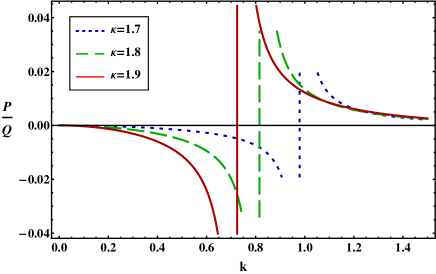
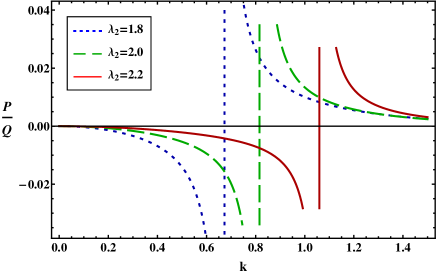
Figure 1: Plot of $P$ vs $k$ for various values of $\kappa$ when $\lambda_{1}=0.7$, $\lambda_{2}=2.0$, $\lambda_{3}=1.5$, and $\lambda_{4}=0.4$.

Figure 2: Plot of $Q$ vs $k$ for various values of $\lambda_{2}$ when $\lambda_{1}=0.7$, $\lambda_{3}=1.5$, $\lambda_{4}=0.4$, and $\kappa=1.8$.

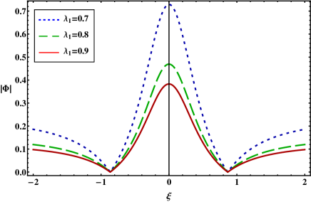
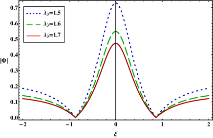
Figure 3: Plot of $|\Phi|$ vs $\xi$ for various values of $\lambda_{1}$, when $\lambda_{2}=2.0$, $\lambda_{3}=1.5$, $\lambda_{4}=0.4$, and $\kappa=1.8$.

Figure 4: Plot of $|\Phi|$ vs $\xi$ for various values of $\lambda_{3}$, when $\lambda_{1}=0.7$, $\lambda_{2}=2.0$, $\lambda_{4}=0.4$, and $\kappa=1.8$.

4 Modulational instability and rogue waves

The nonlinear property of the plasma medium as well as the formation and stability conditions of the DAWs in an EDDPM can be organized according to the sign of dispersive ($P$) and nonlinear ($Q$) coefficients of the standard NLSE (38). The sign of the dispersive coefficient is always negative for any kinds of wave number $k$ in $P$ vs $k$ curve while the sign of the nonlinear coefficient is positive for small values of $k$ and negative for large values of $k$ (figure is not included). Both $P$ and $Q$ have same sign (i.e., positive or negative) then they reflect a modulationally unstable parametric regime (i.e., $P/Q>0$) whereas both $P$ and $Q$ have opposite sign (i.e., positive and negative) then they reflect a modulationally stable parametric regime (i.e., $P/Q<0$) for the DAWs in presence of the external perturbation. The stable and unstable parametric regimes are differentiated by a vertical line at which $P/Q\rightarrow\infty$ (i.e., $Q=0$ and because $P$ is always negative), and the wave number for which $P/Q\rightarrow\infty$ is known as critical waves number ($k_{c}$) [29, 30, 31, 32, 33].

The modulationally unstable parametric regime of the DAWs allows to generate highly energetic and mysterious DARWs associated with DAWs, and the governing equation of the puzzling DARWs can be written as [34, 35]

$$\Phi(\xi,\tau)=\sqrt{\frac{2P}{Q}}\left[\frac{4(1+4iP\tau)}{1+16P^{2}\tau^{2}+4\xi^{2}}-1\right]\mbox{exp}(2iP\tau).$$ (39)

We have numerically analyzed Eq. (39) in Figs. 4 and 4 to understand how the nonlinear properties of a four components EDDPM as well as the configuration of the DARWs associated DAWs have been changed by the various plasma parameters.

5 Results and discussion

The variation of $P/Q$ with $k$ for different values of $\kappa$ as well as the stable and unstable parametric regimes of the DAWs can be observed in Fig. 2, and it is obvious from this figure that (a) DAWs become modulationally stable for small values of $k$ while unstable for large values of $k$; (b) the $k_{c}$ decreases with the increase in the value of the $\kappa$. Figure 2 indicates the effects of the number density as well as the charge state of the positive dust grains and negative ions (via $\lambda_{2}=Z_{1}n_{10}/Z_{+}n_{+0}$) to recognize the stable and unstable parametric regimes of the DAWs, and it can be seen from this figure that (a) the modulationally stable parametric regime increases with $\lambda_{2}$; (b) the modulationally stable parametric regime increases with an increase in the value of negative ion number density ($n_{10}$) while decreases with an increase in the value of the positive dust grains number density ($n_{+0}$) for a constant value of $Z_{1}$ and $Z_{+}$; (c) the modulationally unstable (stable) parametric regime of the DAWs increases with $Z_{+}$ ($Z_{1}$) for a fixed negative ion and positive dust number density.

We have numerically analyzed first-order rogue waves [by using Eq. (39)] in Figs. 4 and 4. Figure 4 highlights the effects of mass of the positive and negative ions as well as their charge states (via $\lambda_{2}=Z_{-}m_{+}/Z_{+}m_{-}$) in recognizing the shape of the DARWs in an electron depleted four components EDDPM, and it can be manifested from this figure that (a) the increase in the value of $\lambda$ does not only cause to change the amplitude of the DARWs but also causes to change the width of the DARWs; (b) the amplitude and width of the DARWs decrease with the increase in the value of $\lambda_{2}$; (c) actually, the nonlinearity of the plasma medium as well as the amplitude of the DARWs increases with increasing $m_{-}$ while the nonlinearity as well as the amplitude of the DARWs decreases with increasing $m_{+}$ for a fixed value of $Z_{+}$ and $Z_{-}$. Figure 4 reflects how the number density and charge state of the light positive ion and heavy negative dust grains (via $\lambda_{3}=Z_{2}n_{20}/Z_{+}n_{+0}$) contribute to generate highly energetic rogue waves in a four components EDDPM. The amplitude and width of the electrostatic DARWs associated with DAWs decreases with an increase in the value of positive ion charge state and number density while increases with an increase in the value of positive dust charge state and number density. The physics of this result is that the nonlinearity of a four components electron depleted plasma medium increases (decreases) with positive dust grain (positive ion) number density as well as with positive dust grain (positive ion) charge state.

6 Conclusion

In this present article, we have examined the modulationally stable and unstable parametric regimes of DAWs, and the DARWs in the unstable parametric regime of DAWs by employing standard NLSE in a four components EDDPM. The numerical analysis can explain the dependency of the stability conditions as well as the configuration of DARWs associated with DAWs in the modulationally unstable parametric regime. To conclude, the results obtained from this investigation should be useful in understanding the basic properties of these rouge waves predicted to be formed in electron depleted unmagnetized opposite polarity dusty plasma systems like mesospherere, F-rings of saturn, and cometary atmosphere, etc.

References

• [1] M. M. Hossen, et al., Eur. Phys. J. D 70, 252 (2016).
• [2] M. M. Hossen, et al., Phys. Plasmas 23, 023703 (2016).
• [3] M. M. Hossen, et al., High Energ. Dens. Phys. 24, 9 (2017).
• [4] P. K. Shukla and V. P. Silin, Phys. Scr. 45, 508 (1992).
• [5] M. Shahmansouri and H. Alinejad, Phys. Plasmas 20, 033704 (2013).
• [6] N. N. Rao, et al., Planet. Space Sci. 38, 543 (1990).
• [7] A. Barkan, et al., Phys. Plasmas 2, 3563 (1995).
• [8] P. K. Shukla, et al., J. Geophys. Res. 96, 21343 (1991).
• [9] F. Melandso, Phys. Plasmas 3, 3890 (1996).
• [10] M. Ferdousi, et al., Astrophys. Space Sci. 43, 360 (2015).
• [11] A. A. Mamun, et al., Phys. Plasma 3, 702 (1996).
• [12] K. Dialynas, et al., J. Geophys. Res. 114, A01212 (2009).
• [13] S. Mayout and M. Tribeche, J. Plasma Phys. 78, 657 (2012).
• [14] B. Sahu and M. Tribeche, Astrophys. Space Sci. 341, 573 (2012).
• [15] M. Ferdousi, et al., Eur. Phys. J. D. 71, 102 (2017).
• [16] V. M. Vasyliunas, J. Geophys. Res. 73, 2839 (1968).
• [17] M. J. Uddin, et al., Phys. Plasmas 22, 062111 (2015).
• [18] M. Shahmansouri and H. Alinejad, Phys. Plasmas 19, 123701 (2012).
• [19] I. Kourakis and S. Sultana, AIP Conf. Proc. 1397, 86 (2011).
• [20] S. Sultana, et al., Plasma Phys. Control. Fusion 53, 045003 (2011).
• [21] N. Ahmed, et al., Chaos 28, 123107 (2018).
• [22] T. S. Gill, et al., Phys. Plasmas 17, 013701 (2010).
• [23] N. S. Saini and I. Kourakis, Phys. Plasmas 15, 123701 (2018).
• [24] N. A. Chowdhury, et al., Chaos 27, 093105 (2017).
• [25] M. H. Rahman, et al., Chinese J. Phys. 56, 2061 (2018).
• [26] N. A. Chowdhury, et al., Phys. plasmas 24, 113701 (2017).
• [27] M. H. Rahman, et al., Phys. Plasmas 25, 102118 (2018).
• [28] N. A. Chowdhury, et al., Vacuum 147, 31 (2018).
• [29] R. K. Shikha, et al., Eur. Phys. J. D 73, 177 (2019).
• [30] N. A. Chowdhury, et al., Plasma Phys. Rep. 45, 459 (2019).
• [31] S. Jahan, et al., Commun. Theor. Phys. 71, 327 (2019).
• [32] N. A. Chowdhury, et al., Contrib. Plasma Phys. 58, 870 (2018).
• [33] M. Hassan, et al., Commun. Theor. Phys. 71, 1017 (2019).
• [34] N. Akhmediev, et al., Phys. Rev. E 80, 026601 (2009).
• [35] A. Ankiewicz, et al., Phys. Lett. A 373, 3997 (2009).