Chemical Abundances in a Turbulent Medium – H₂, OH⁺, H₂O⁺, ArH⁺

Abstract

Supersonic turbulence results in strong density fluctuations in the interstellar medium (ISM), which have a profound effect on the chemical structure. Particularly useful probes of the diffuse ISM are the ArH⁺, OH⁺, H₂O⁺ molecular ions, which are highly sensitive to fluctuations in the density and the H₂ abundance. We use isothermal magnetohydrodynamic (MHD) simulations of various sonic Mach numbers, $\mathcal{M}_{s}$, and density decorrelation scales, $y_{\rm dec}$, to model the turbulent density field. We post-process the simulations with chemical models and obtain the probability density functions (PDFs) for the H₂, ArH⁺, OH⁺ and H₂O⁺ abundances. We find that the PDF dispersions increases with increasing $\mathcal{M}_{s}$ and $y_{\rm dec}$, as the magnitude of the density fluctuations increases, and as they become more coherent. Turbulence also affects the median abundances: when $\mathcal{M}_{s}$ and $y_{\rm dec}$ are high, low density regions with low H₂ abundance become prevalent, resulting in an enhancement of ArH⁺ compared to OH⁺ and H₂O⁺. We compare our models with Herschel observations. The large scatter in the observed abundances, as well as the high observed ArH⁺/OH⁺ and ArH⁺/H₂O⁺ ratios are naturally reproduced by our supersonic $(\mathcal{M}_{s}=4.5)$, large decorrelation scale $(y_{\rm dec}=0.8)$ model, supporting a scenario of a large-scale turbulence driving. The abundances also depend on the UV intensity, CR ionization rate and the cloud column density, and the observed scatter may be influenced by fluctuations in these parameters.

1. Introduction

A diverse collection of molecules and molecular ions has been detected in the interstellar medium (ISM). The abundances of observed species and their ratios are often used to constrain cloud properties: the temperature, incident ultraviolet (UV) radiation flux, cosmic-ray ionization rate (CRIR), and the density of H nuclei, $n\equiv n({\rm H})+2n({\rm H_{2}})$.

Diffuse clouds in the ISM are commonly analyzed by chemical models for photodissociation-regions (PDRs; e.g., Kaufman et al. 1999; Tielens & Hollenbach 2002; Sternberg & Dalgarno 1995; Bell et al. 2006; Röllig et al. 2006; Le Petit et al. 2006). Neufeld & Wolfire (2016, hereafter NW) used constant-$n$ PDR models to study the abundances of ArH⁺, OH⁺, and H₂O⁺, and compared their model predictions with observations. These molecular-ions are sensitive to the H₂ abundance, which in turn depends on the the UV intensity, the CRIR, the cloud visual extinction, and the gas density. NW showed that for all sightlines, there is a discrepancy between their theoretical models and the observations, as the models always under-predict the ArH⁺ abundance relative to OH⁺ and H₂O⁺. To explain this discrepancy, they were forced to invoke a two-cloud population model in which low $A_{\rm V}$ clouds were the source for the ArH⁺, while higher $A_{\rm V}$ clouds produced the OH⁺ and H₂O⁺. Furthermore, the observations show scatter in the column density ratios $N({\rm ArH^{+}})/N({\rm H})$, $N({\rm OH^{+}})/N({\rm H})$, and $N({\rm H_{2}O^{+}})/N({\rm H})$, for different lines-of-sight (LoS). NW attributed the scatter to variations in the CRIR.

A common simplifying assumption in PDR models is that the gas density in the cloud is constant (or is smoothly varying with cloud depth). However, this assumption may be wrong. Observations suggest that molecular clouds as well as cold atomic clouds exhibit turbulent supersonic motions, as is evident from, e.g.: the observed superthermal linewidths, the line-width size relation, the fractal structures of molecular clouds, and studies of the power spectrum/bispectrum (e.g., Vazquez-Semadeni, 1994; Stutzki et al., 1998; Sanchez et al., 2005; Heyer et al., 2009; Burkhart et al., 2009; Roman-Duval et al., 2010; Chepurnov et al., 2015). The turbulence, when supersonic, produces strong density fluctuations in the gas, which alter the chemical structure.

Bialy et al. (2017b, hereafter BBS) have shown that in a turbulent medium, density fluctuations perturb the H and H₂ abundances in the gas, resulting in large dispersions in the atomic columns, $N({\rm H})$, for different LoS. The variance in the $N({\rm H})$ distribution was related to the governing turbulent parameters: the sonic Mach number, $\mathcal{M}_{s}$, and the decorrelation scale of the density field, $L_{\rm dec}$, which is proportional to the turbulence driving scale, $L_{\rm drive}$.

In this paper we extend upon the NW and BBS analyses. We study how turbulence affects the abundances of H₂, ArH⁺, OH⁺, and H₂O⁺, and compare our models with observations. We find that our turbulent-cloud models may explain the observed scatter in the observed abundances, as well as the high ArH⁺/OH⁺ and ArH⁺/H₂O⁺ ratios. We demonstrate how the observations may be used to constrain the turbulent parameters, $\mathcal{M}_{s}$ and $L_{\rm drive}$.

The paper is organized as follows. In §2 we review the chemical network and discuss the governing physical parameters. In §3 we discuss the model ingredients, including our MHD simulations and the chemical PDR models. In §4 we present our results for the abundance distributions in turbulent clouds. In §5 we compare our models with observations. We discuss the limitations of the model and our conclusions in §6 and §7.

2. Chemistry

The formation and destruction pathways include two-body reactions, surface chemistry on dust-grains, and cosmic-ray and UV photoreactions. We define the abundance of species $i$, $x({\rm i})\equiv n({\rm i})/n$, where $n(i)$ is the density of species $i$, and $n$ is the density of hydrogen nuclei.

2.1. H and H₂

The H₂ is formed on the surfaces of dust grains. The removal of H₂ is through photodissociation by Lyman-Werner (LW) radiation (11.2-13.6 eV), and by cosmic-ray (CR) ionization. The H and H₂ steady-state abundances obey

$$\frac{x({\rm H_{2}})}{x({\rm H})}=\frac{Rn}{D_{0}f_{\rm att}+\zeta_{\rm tot}}\ ,$$ (1)

and by element conservation, $x({\rm H})+2x({\rm H_{2}})\simeq 1$. Here, $R=3\times 10^{-17}$ cm³ s^-1 is the H₂ formation rate coefficient for formation on dust-grains (the value is for a 100 K gas), and $D_{0}=5.8\times 10^{-11}I_{\rm UV}$ s^-1 (Sternberg et al., 2014), where $I_{\rm UV}$ is the interstellar radiation field in units of the value given by Draine (1978). The attenuation factor, $f_{\rm att}$, accounts for the absorption of LW photons by dust and in H₂ lines. For normal incidence radiation, penetrating a slab on two sides

$$f_{\rm att}=\frac{1}{2}f_{\rm sh}(N^{l}({\rm H_{2}}))\mathrm{e}^{-\sigma_{g}N^{l}}+\frac{1}{2}f_{\rm sh}(N^{r}({\rm H_{2}}))\mathrm{e}^{-\sigma_{g}N^{r}}\ .$$ (2)

Here $\sigma_{g}=1.9\times 10^{-21}$ cm² is the dust absorption cross section per hydrogen nucleus (Sternberg et al., 2014), and $f_{\rm sh}$ is the H₂ self-shielding function (Eq. 37 in Draine & Bertoldi, 1996) for which we adopt $b=2$ km/s (see §6.4 and appendix A). $N$ and $N({\rm H_{2}})$ are the column densities of hydrogen nuclei and H₂, from cloud edge to the point of interest, and the superscripts $l$ and $r$ denote integration from the left and right cloud edges, respectively.

In Eq. (1), $\zeta_{\rm tot}\approx 2.3\times 1.9\times\zeta$ is the total CR removal rate of H₂ and where $\zeta$ is the primary CRIR of H. The factor $2.3$ translates from primary CR ionization per H to total (primary+secondary) ionization per H₂ (Glassgold & Langer, 1974), and the additional factor $1.9$ accounts for H₂ destruction by chemical reactions with molecular ions which are produced by CR ionization (i.e., the H₂ abstraction reactions below). We define $\zeta_{-16}\equiv\zeta/(10^{-16}{\rm s^{-1}})$

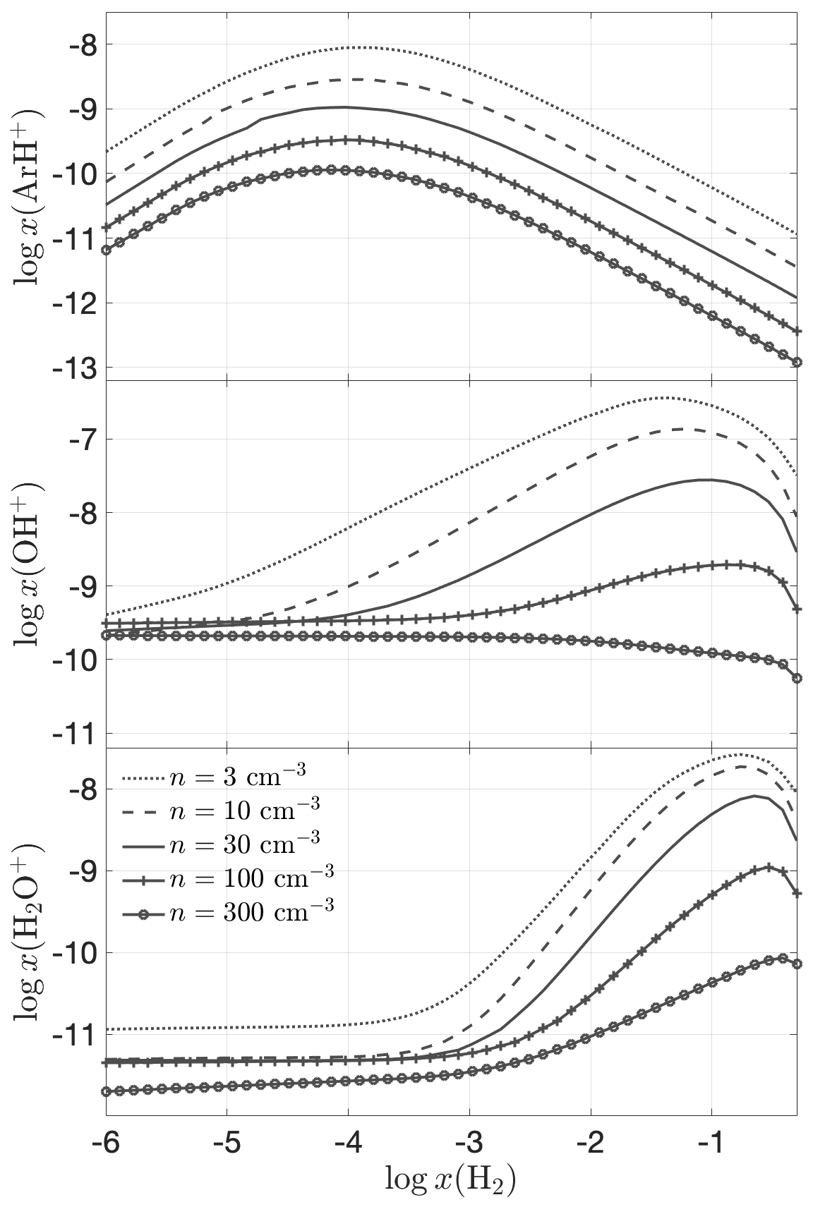
Figure 1.— The ArH⁺, OH⁺, and H₂O⁺ abundances ($x(i)\equiv n(i)/n$) as functions of the H₂ abundance, for $I_{\rm UV}=1$, $\zeta_{-16}=4$, and various (constant) densities $n$.

2.2. ArH⁺, OH⁺, and H₂O⁺

Here we discuss the basic formation and destruction chemistry for ArH⁺, OH⁺, and ${\rm H_{2}O^{+}}$ (see also Schilke et al. 2014 and NW). The production of ArH⁺ is initiated by CR ionization followed by hydrogen abstraction

$${\rm Ar}+{\rm cr} \rightarrow{\rm Ar^{+}}+{\rm e}\ ,$$ (3)

$${\rm Ar^{+}}+{\rm H_{2}} \rightarrow{\rm ArH^{+}}+{\rm H}\ .$$ (4)

The formation sequence is moderated by the recombination of Ar⁺ with polycyclic aromatic hydrocarbons (PAH), and PAH^- (dielectric recombination is subdominant, Arnold et al., 2015). Dissociative recombination of ArH+ is unusually slow (NW), and its destruction is dominated by proton transfer with H₂

$${\rm ArH^{+}}+{\rm H_{2}}\rightarrow{\rm Ar}+{\rm H_{3}^{+}}\ .$$ (5)

If the H₂ abundance is low, $x({\rm H_{2}})\lesssim 10^{-4}$, the removal of ${\rm ArH^{+}}$ proceeds mainly through charge transfer with O and C.

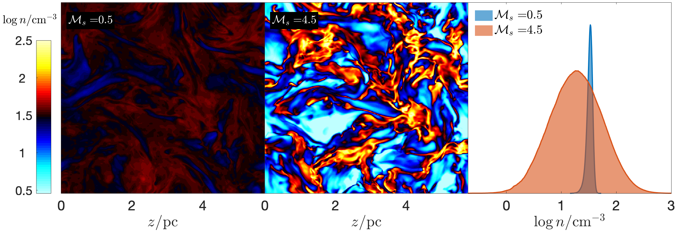
Figure 2.— Density cuts through the $\mathcal{M}_{s}=0.5$ and $4.5$ simulations (with $y_{\rm dec}=0.08$), and the corresponding density PDFs.

The production of ${\rm OH^{+}}$ is initiated by CR ionization of H, followed by charge transfer and H abstraction,

$${\rm H}+{\rm cr} \rightarrow{\rm H^{+}}+{\rm e}\ ,$$ (6)

$${\rm H^{+}}+{\rm O} \rightarrow{\rm O^{+}}+{\rm H}\ ,$$ (7)

$${\rm O^{+}}+{\rm H_{2}} \rightarrow{\rm OH^{+}}+{\rm H}\ .$$ (8)

If the H₂ abundance is sufficiently high, OH⁺ is formed through the sequence

$${\rm H_{2}}+{\rm cr} \rightarrow{\rm H_{2}^{+}}+{\rm e}\ ,$$ (9)

$${\rm H_{2}^{+}}+{\rm H_{2}} \rightarrow{\rm H_{3}^{+}}+{\rm H}\ ,$$ (10)

$${\rm H_{3}^{+}}+{\rm O} \rightarrow{\rm OH^{+}}+{\rm H_{2}}\ .$$ (11)

Further abstraction reactions with H₂ destroy OH⁺ and lead to the formation of H₂O⁺ and H₃O⁺

$${\rm OH^{+}}+{\rm H_{2}} \rightarrow{\rm H_{2}O^{+}}+{\rm H}\ ,$$ (12)

$${\rm H_{2}O^{+}}+{\rm H_{2}} \rightarrow{\rm H_{3}O^{+}}+{\rm H}\ .$$ (13)

OH+ and H2O+ are also destroyed by dissociative recombination and photodissociation (see Fig. 2 in Bialy & Sternberg 2015).

Because of the abstraction reactions with H₂, the OH⁺ and H₂O⁺ abundances are very sensitive to $x({\rm H_{2}})$, down to very low H₂ abundances, $x({\rm H_{2}})\sim 10^{-3}-10^{-4}$. At still lower ${\rm H_{2}}$ abundances, OH⁺ and H₂O⁺ are formed via solid-state chemistry on dust grains (Hollenbach et al., 2012; Sonnentrucker et al., 2015), and their abundances are independent of $x({\rm H_{2}})$. In this regime, atomic hydrogen on grains reacts with atomic oxygen to form OH. The OH can be desorbed from the grain surface or react with another hydrogen to form ${\rm H_{2}O}$. Upon desorption, OH and ${\rm H_{2}O}$ undergo a charge transfer with ${\rm H^{+}}$ forming ${\rm OH^{+}}$ and ${\rm H_{2}O^{+}}$.

In Fig. 1 we show the ${\rm ArH^{+}}$, ${\rm OH^{+}}$ and ${\rm H_{2}O^{+}}$ abundances as functions of $x({\rm H_{2}})$, as computed by our PDR models (see §3.1 below) for $I_{\rm UV}=1$, $\zeta_{-16}=4$, and for various densities, $n$. For a fixed $x({\rm H_{2}})$ the abundances of all the molecular ions increase with decreasing $n$. The formation rate is proportional to $\zeta$, while destruction is proportional to $n$, so all three molecular ions have abundances that increase with $\zeta/n$.

At a constant $n$, the $x({\rm ArH^{+}})$ is a non-monotonic function of $x({\rm H_{2}})$: it increases with $x({\rm H_{2}})$ when $x({\rm H_{2}})$ is very small, peaks at $x({\rm H_{2}})\sim 10^{-4}$, and then decreases with $x({\rm H_{2}})$. This behavior may be understood as follows. When $x({\rm H_{2}})$ is very small, the abstraction reaction (4) is slow, and is heavily interrupted by Ar⁺ recombinations with PAHs. As a result, the formation rate is $\propto\zeta$ multiplied by a branching ratio $\propto x({\rm H_{2}})$. Destruction, on the other hand, is dominated by charge transfer with O and C, and is independent of $x({\rm H_{2}})$. Thus the abundance scales with $x({\rm H_{2}})$. At high $x({\rm H_{2}})$, the abstraction reaction proceeds rapidly such that every Ar ionization leads to the formation of ArH⁺, and the formation is independent of $x({\rm H_{2}})$. However, removal is now dominated by interactions with H₂. Thus the overall abundance scales inversely with $x({\rm H_{2}})$. Similar considerations explain the non-monotonic behavior of the OH⁺ and H₂O⁺ abundances.

3. Model Ingredients

3.1. Chemical PDR Models

We ran a large series of chemical PDR models similar to those described by Wolfire et al. (2010) and Hollenbach et al. (2012, with updates as described in NW). Each model is characterized by (1) $I_{\rm UV}/n$, (2) $\zeta/n$, and (3) total visual extinction, $A_{\rm V}$, through the cloud (denoted $A_{\rm V}{\rm(tot)}$ by NW). The models span the parameter space $I_{\rm UV}/n=20$ to $10^{-3}$ cm³, $\zeta/n=10^{-20}$ to $4\times 10^{-16}$ cm³ s^-1, and $A_{\rm V}=3\times 10^{-4}$ to $8$ mag. For any given set of parameters, the model computes the temperature and molecular abundances (assuming steady-state) as functions of cloud depth, hereafter the $z$ coordinate.

Generally the fractional densities inside the cloud, $x(i)$, depend on the four parameters, $I_{\rm UV}/n$, $\zeta/n$, the total cloud visual extinction $A_{\rm V}$, and cloud depth $z$. However, for ArH⁺, OH⁺, and H₂O⁺, the dependence on $z$ and $A_{\rm V}$ is fully captured by the variation of the H₂ fraction, $x({\rm H_{2}})$. To this end, we re-express the molecular-ion abundances as functions of $x({\rm H_{2}})$, reducing the rank of the parameter-space by 1 ($\{z,A_{\rm V}\}\rightarrow x({\rm H_{2}})$). We construct lookup tables for $x(i)$ ($i={\rm ArH^{+},OH^{+},H_{2}O^{+}}$) as functions of $I_{\rm UV}/n$, $\zeta/n$ and $x({\rm H_{2}})$.

3.2. MHD Simulations

To model the density field in the turbulent medium, we solve the ideal MHD equations

$$\frac{\partial\rho}{\partial t}+\nabla\cdot(\rho\boldsymbol{\varv}) =0\ ,$$ (14)

$$\frac{\partial\rho\boldsymbol{\varv}}{\partial t}+\nabla\cdot\left[\rho\boldsymbol{\varv}\boldsymbol{\varv}+\left(p+\frac{B^{2}}{8\pi}\right){\bf I}-\frac{1}{4\pi}{\bf B}{\bf B}\right] ={\bf f}\ ,$$ (15)

$$\frac{\partial{\bf B}}{\partial t}-\nabla\times(\boldsymbol{\varv}\times{\bf B}) =0\ .$$ (16)

Here $\rho$ is density, ${\bf B}$ is magnetic field, $p$ is the gas pressure, ${\bf I}$ is the identity matrix and $\bf{f}$ is the specific force. We use a third-order-accurate hybrid essentially nonoscillatory scheme on a 3D grid of 512³ cells. The $B$ field is initially aligned along the $y$ axis. We assume periodic boundary conditions, and an isothermal equation of state $p=c_{s}^{2}\rho$. By constrained transport we numerically construct $\nabla\cdot{\bf B}=0$. For the source term $\bf{f}$, we assume a random large-scale solenoidal driving at a wave number $k\approx 2.5$ (i.e. 1/2.5 the box size). For more details see Burkhart et al. (2009).

Each simulation is defined by two parameters, the sonic and Alfvénic Mach numbers, $\mathcal{M}_{s}\equiv\langle|\boldsymbol{\varv}|\rangle/c_{s}$, $\mathcal{M}_{A}\equiv\langle|\boldsymbol{\varv}|\rangle/\varv_{A}$, where $\boldsymbol{\varv}$ is the velocity, $c_{s}$ and $\varv_{A}$ are the isothermal sound speed and the Alfvén speed, and $\langle\cdot\rangle$ denotes averages over the entire simulation box. We consider three simulations, $\mathcal{M}_{s}=0.5$, 2.0 and 4.5, corresponding to subsonic, transonic, and supersonic medium. All simulations have $\mathcal{M}_{A}=2$. As discussed in BBS, $\mathcal{M}_{s}$ strongly affects the variance of the density field, and hence the H-H₂ structure. However, the H-H₂ structure is only weakly sensitive to the Alfvénic number. As the simulations do not include gravity and chemistry the density and size are scale-free (see Appendix in Hill et al., 2008). We adopt $L_{\rm cloud}=6.3$ pc for the simulation box length, and $\langle n\rangle=30$ cm^-3, corresponding to a mean cloud column $\langle N\rangle\equiv\langle n\rangle L_{\rm cloud}=5.8\times 10^{20}$ cm^-2 or $\langle A_{\rm V}\rangle=0.3$ mag.

In Figure 2 we show density slices, and density PDFs, for the $\mathcal{M}_{s}=0.5$ and 4.5 simulations. The density is nearly homogeneous in the subsonic simulation, while in the supersonic case shocks develop and lead to strong density fluctuations in the gas. The $n$-PDF is close to a lognormal, with a dispersion that increases with the sonic Mach number, as $\sigma_{\ln(n/\langle n\rangle)}^{2}\simeq\ln[1+(b\mathcal{M}_{s})^{2}]$, where $b=1/3$ is the forcing parameter (Federrath et al., 2008).

The large-scale driving yields a density field that is correlated over large scales. The decorrelation scale in the simulation is $y_{\rm dec}\equiv L_{\rm dec}/L_{\rm cloud}=0.08$, i.e., $\approx 40$ cells (BBS). $L_{\rm dec}$ is the characteristic scale over which correlations in the density field decrease: For averaging over length $L$, the density variance decreases with increasing $L$, and $L_{\rm dec}$ is the characteristic scale for this decreasing trend (see §4.2 in BBS. cf. Vazquez‐Semadeni & Garcia 2001 for alternative definitions). In supersonic gas, density fluctuations are still present on scales below $L_{\rm dec}$, all the way down to the sonic-length, $L_{s}$ (see footnote 10 below). As evident in Fig. 2, $L_{\rm dec}$ is indeed a typical length-scale for the large-scale density modes in the simulations. The value of $y_{\rm dec}$ has a strong influence on the resulting chemical structure (see §4.2.1 below). To study the effects of variations in $y_{\rm dec}$, we crop each of the simulations after 51 cells, producing thin slabs of thickness $1/10$ of the original boxes. The relative decorrelation length in the slabs (along the short axes) is $y_{\rm dec}\simeq 0.8$. The slab thickness is still set to $L_{\rm cloud}=6.3$ pc, as for the original simulation boxes.

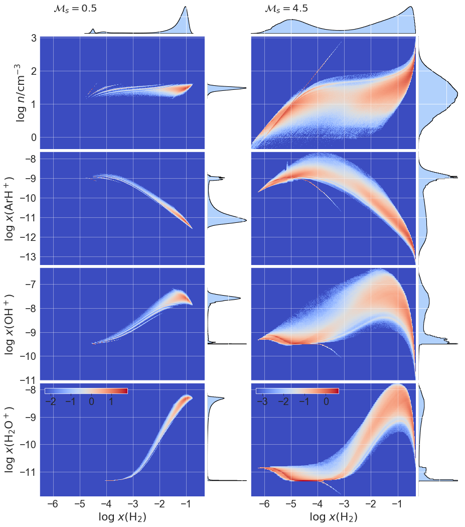
Figure 3.— The joint-PDFs of $x({\rm H_{2}})$ versus $n$, $x({\rm ArH^{+}})$, $x({\rm OH^{+}})$ and $x({\rm H_{2}O^{+}})$, for the $\mathcal{M}_{s}=0.5$ (left) and 4.5 (right) simulation boxes, with $y_{\rm dec}=0.08$, and $I_{\rm UV}=1$, $\zeta_{-16}=4$, $\langle n\rangle=30$ cm^-3, $\langle A_{\rm V}\rangle=0.3$. The colors corresponds to $\log$ of the PDF, as indicated (each of the colorbars applies to the entire column). The marginal PDFs (in linear scale) are also shown. The stratification seen in the left panels is an artifact resulting from the finite size of simulation cells. In our chemical computations, we use a much finer (logarithmic) grid, and then we interporlate the results onto the simulation boxes.

3.3. Numerical Procedure

As our focus is on the effects of turbulence, we fix the non-turbulent parameters $I_{\rm UV}=1$, $\zeta_{-16}=4$, $\langle n\rangle=30$ cm^-3 and $\langle A_{\rm V}\rangle=0.3$, and study the dependence on the turbulent parameters $\mathcal{M}_{s}$ and $y_{\rm dec}$. The effects of $I_{\rm UV}$, $\zeta$ and $A_{\rm V}$ are studied in NW. The LoS direction from the observer to the cloud (simulation) along which we integrate the column is aligned with the $z$ axis. $z$ is also the axis along which the radiation propagates (i.e., as we assume slab geometry). In the Appendix we explored other LoS orientations, along $x$ or $y$, and find that the results are weakly sensitive to the LoS direction.

We post process each of the simulations as follows:

1. The 3D density field, $n(x,y,z)$, is used as an input to the chemical model.

2. For each LoS, $(x,y)$, we solve Eqs. (1-2) on a fine logarithmic grid, and then interpolate the results back onto the simulation box.

3. Given $x({\rm H_{2}})(x,y,z)$ and $n(x,y,z)$, we use the lookup tables to obtain the ArH⁺, OH⁺ and H₂O⁺ abundances in all the cells, $x(i)(x,y,z)$.

4. We also integrate the abundances along the LoS direction, $z$, yielding the species column densities for all LoS, $N(i)(x,y)$.

We now have the abundance and column density PDFs for the six cases: $\mathcal{M}_{s}=(0.5,2,4.5)$ for $y_{\rm dec}=(0.08,0.8)$.

4. Results

In this section we present the probability distribution functions (PDFs) of the abundances $x(i)$, and the columns, $N(i)$.

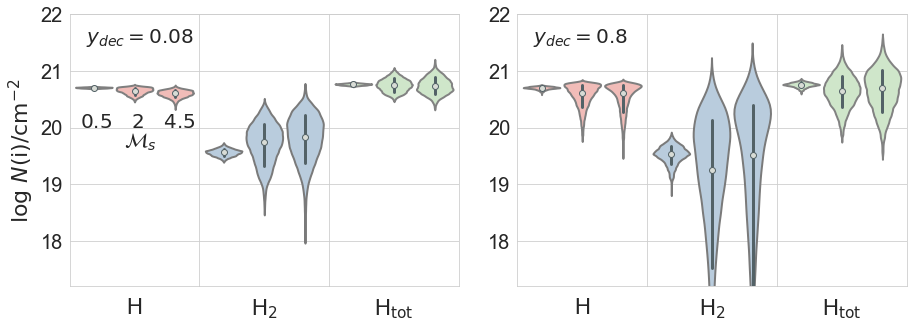
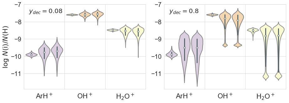
Figure 4.— Violin plots (where the width along the $x$ axis is $\propto$ probability density) of the H, H₂ and H_tot columns (top), and the ArH⁺ OH⁺ and H₂O⁺ columns relative to the H column (bottom), for simulations with $y_{\rm dec}=0.08$ (left) and $y_{\rm dec}=0.8$ (right), assuming $I_{\rm UV}=1$, $\zeta_{-16}=4$, $\langle n\rangle=30$ cm^-3, $\langle A_{\rm V}\rangle=0.3$. For each species, the triplet of violins corresponds to $\mathcal{M}_{s}=0.5,2,4.5$, as indicated. For each violin, the white point, vertical line, and total vertical length, correspond to the median, and the 68 and 99.7 percentile ranges about the median, respectively.

4.1. Abundance PDFs

To demonstrate the effect of the density fluctuations on the chemical structure, in Fig. 3 we plot the joint-PDFs for $n$, $x({\rm ArH^{+}})$, $x({\rm OH^{+}})$ and $x({\rm H_{2}O^{+}})$ with $x({\rm H_{2}})$, and their marginal PDFs, for the subsonic $\mathcal{M}_{s}=0.5$ (left) and the supersonic $4.5$ (right) simulations (both with $y_{\rm dec}=0.08$). In the subsonic case the density PDF is narrow, with most cells having density $n\approx\langle n\rangle=30$ cm^-3. The H₂ distribution exhibits a spread, from $\log x({\rm H_{2}})\sim-5$ to $-1$, corresponding to regions near cloud boundaries and center. The ArH⁺, OH⁺ and H₂O⁺ PDFs as functions of $x({\rm H_{2}})$ follow the shapes of the constant density $n=30$ cm^-3 models (see Fig. 1), as they should.

In the supersonic case, strong density fluctuations are developed, and the $n$ PDF is wide. The onset of H₂ self-shielding leads to a rapid growth in $x({\rm H_{2}})$ with increasing cloud depth (column density) resulting in a bimodal PDF. At a given depth, higher gas densities result in more efficient H₂ formation and thus a positive correlation between $x({\rm H_{2}})$ and $n$. At cloud boundaries, the correlation is linear, with $x({\rm H_{2}})=Rn/(D_{0}/2)$. This is evident as the thin diagonal density enhancement extending from $\log x({\rm H_{2}}),\log n=(-3,3)$ to $(-6,0)$. For $n\lesssim 10$ cm^-3, there is an additional density enhancement, which also extends diagonally, but at an offset of factor of 2 to the left. This corresponds to LoS that are so diffuse that radiation from the far side of the cloud penetrates, resulting in a factor of 2 higher dissociation rate.

The density fluctuations in the $\mathcal{M}_{s}=4.5$ simulation enhance the dynamic range of $x({\rm H_{2}})$ and thus the dynamic ranges of ArH⁺, OH⁺ and H₂O⁺. At a given $x({\rm H_{2}})$, the density fluctuations also lead to a spread in the ArH⁺, OH⁺ and H₂O⁺ PDFs, through their dependencies on $\zeta/n$. Since $x({\rm H_{2}})$ and $n$ are correlated, the PDF peaks as functions of $x({\rm H_{2}})$ no longer follow any of the constant density models. For example, as $x({\rm H_{2}})$ increases from $10^{-4}$ to 0.5, the ArH⁺ falls from $\approx 10^{-9}$ to $\lesssim 10^{-13}$, which correspond to the $n=30$ and 300 cm^-3 models in Fig. 1, respectively.

The marginal PDFs of the molecular ions are composed of a broad and a narrow component. In the case of OH⁺ and H₂O⁺ the narrow components correspond to formation on dust near cloud boundaries (where $x({\rm H_{2}})$ is small) which lead to characteristic OH⁺ and H₂O⁺ abundances, that depend weakly on $x({\rm H_{2}})$ or $n$. In the case of ArH⁺, the narrow PDF reflects the maximum in the $x({\rm ArH^{+}})$ versus $x({\rm H_{2}})$ relation (which occurs at $x({\rm ArH^{+}})\sim 10^{-9}$ for $\langle n\rangle=30$ cm^-3).

4.2. Column Density PDFs

In Fig. 4 we show the column density (or column density ratios) PDFs in the form of violin charts (where the width is proportional to the PDF dispersion), as obtained for all of our simulations, $\mathcal{M}_{s}=0.5,2$ and $4.5$, for $y_{\rm dec}=0.08$ (left) and 0.8 (right).

All PDF widths increase with increasing $\mathcal{M}_{s}$ as a result of the density fluctuations. The widths vary among species as is determined by the individual dependencies of $x(i)$ on $n$ (see §4.1). The column PDFs are further affected by the density as cells with higher density contribute more to the column, $N(i)=\int x(i)n\mathrm{d}z$. For example, the $N({\rm H})$ PDFs are all very narrow because $x({\rm H})$ is anti-correlated with $n$, thus the cells where $x({\rm H})$ is high have a low contribution to $N({\rm H})$, and vice versa. By contrast, $x({\rm H_{2}})$ correlates with $n$, and thus the $N({\rm H_{2}})$ PDFs are very wide.

The medians also show a dependence on $\mathcal{M}_{s}$. The median ArH⁺ increases with $\mathcal{M}_{s}$, both at $y_{\rm dec}=0.8$ and 0.08. This is because the density field is characterized by a lognormal PDF in which low densities are more common than high (i.e., $n_{\rm med}<\langle n\rangle$). These diffuse regions are deficient in H₂, and thus enhanced in ArH⁺, leading to an overall increase in the median ArH⁺ value. This is evident by comparing the $\mathcal{M}_{s}=0.5$ and 4.5 abundance PDFs in Fig. 3. For $y_{\rm dec}=0.8$, the median OH⁺ and H₂O⁺ decrease with increasing $\mathcal{M}_{s}$, as the H₂-poor gas depresses OH⁺ and H₂O⁺ formation.

At small $y_{\rm dec}$, the trends with $\mathcal{M}_{s}$ are less pronounced as there are many density fluctuations along the sightlines, which, upon summation, partially cancel out (see §4.2.1 below). The sum is not evenly weighted as cells with high density contribute more to the total integrated column. This is the reason why the median OH⁺ trend is reversed at $y_{\rm dec}=0.08$: While $x({\rm OH^{+}})$ is depressed in the low $x({\rm H_{2}})$ (low $n$) regions, the depression is sufficiently weak so that the $x({\rm OH^{+}})$-rich (high $n$) regions are able to (over)compensate through the larger weight they have in the integrated column.

4.2.1 The Role of $y_{\rm dec}$

The PDFs in Fig. 4 depend strongly on the decorrelation scale, $y_{\rm dec}$ (see discussion in §3.2). Most prominent is the increase in the PDF dispersions as $y_{\rm dec}$ increases. This is because when $y_{\rm dec}$ is large, the density fluctuations are coherent along the LoS (the number of fluctuations $\sim 1/y_{\rm dec}$). Since the density still varies between LoS, there are large variations in the abundances among the sightlines and the PDFs are wide. On the other hand, when $y_{\rm dec}$ is small, each LoS contains several ($\sim 10$) density fluctuations along it. Upon integration, positive and negative fluctuations average-out, resulting in narrower PDFs. The H₂ PDF is particularly wide in the $y_{\rm dec}=0.8$ case, because at any point in the cloud, the H₂ is affected by all cells along the LoS through H₂ self-shielding and thus coherent density fluctuations strongly affect H₂.

Generally, because at large $y_{\rm dec}$ the density field is more coherent, the column PDFs more closely resemble the $x(i)$ PDFs, in this limit. For example, in the $y_{\rm dec}=0.8$ case the OH⁺ and H₂O⁺ PDFs both have peaks at low values (at $\log N({\rm i})/N({\rm H})\approx-9.3$ and $-11.1$), which are absent in the $y_{\rm dec}=0.08$ case. These peaks correspond to low-density clouds with low $x({\rm H_{2}})$, in which the OH⁺ and H₂O⁺ are formed through the dust-catalysis formation routes, reflecting the narrow peaks in the $x(i)$ PDFs in Fig. 3. For $y_{\rm dec}=0.08$, these features disappear as the low-$x(i)$ regions are averaged over with regions with higher $x(i)$, where the high-$x(i)$ regions have a larger weight.

The dependence of PDF width on $y_{\rm dec}$ may be understood analytically for the case of the $N$ PDF (also in the case of $N({\rm H})$, see BBS). Following BBS, we approximate the density field in two cells along the LoS as (a) two uncorrelated variables if $\Delta z>L_{\rm dec}$ where $\Delta z$ is the seperation along the LoS, or (b) assume full correlation if $\Delta z<L_{\rm dec}$ . The number of fluctuations along a LoS is then

$$\mathcal{N}=1+1/y_{\rm dec}\ .$$ (17)

In this approximation, the column density is the sum of $\mathcal{N}$ independent variables, and its standard deviation obeys

$$\sigma_{N/\langle N\rangle}\simeq\frac{\sigma_{n/\langle n\rangle}}{\sqrt{\mathcal{N}}}\simeq\frac{b\mathcal{M}_{s}}{\sqrt{1+1/y_{\rm dec}}}\ .$$ (18)

The PDF dispersion increases with $\mathcal{M}_{s}$ and with increasing fluctuation size, $y_{\rm dec}$ (or with decreasing $\mathcal{N}$). Eq. (18) is in 10-30% agreement with our numerically calculated standard deviations for all six simulations.

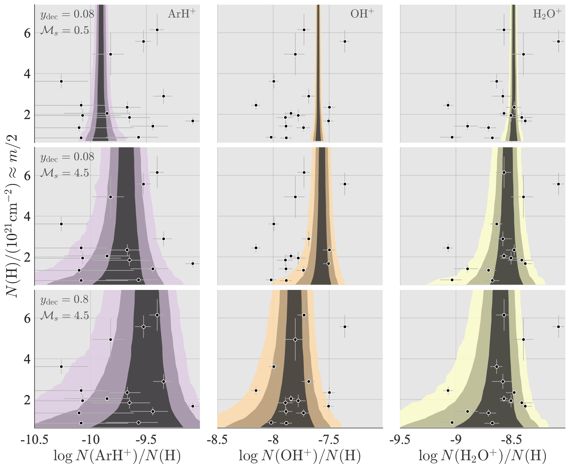
Figure 5.— The grand PDFs of ${\rm ArH^{+},OH^{+},H_{2}O^{+}}$ as functions of $N({\rm H})$ (which is $\propto$ to the number of clouds along the LoS, $m$.), for different ($y_{\rm dec},\mathcal{M}_{s}$) combinations. All models assume $I_{\rm UV}=1$, $\zeta_{-16}=4$, $\langle n\rangle=30$ cm^-3, $\langle A_{\rm V}\rangle=0.3$. In each panel, the three shaded regions correspond to the 68, 95, 99.7 percentiles about the median (at constant $N({\rm H})$). The observations are indicated by dots with errorbars.

In the limit $y_{\rm dec}\gg 1$, $\sigma_{N/\langle N\rangle}\rightarrow\sigma_{n/\langle n\rangle}$ independent of $y_{\rm dec}$. In this limit, each cloud corresponds to a single density fluctuation in the large-scale density field. The column PDF of species may then be obtained directly from the uniform density models, weighting each model with the $n$-PDF.

The decorrelation scale is related to the driving scale:

$$L_{\rm dec}=\phi L_{\rm drive}\ ,$$ (19)

or in dimensionless units, $y_{\rm dec}=\phi(L_{\rm drive}/L_{\rm cloud})$. In our simulations $\phi=0.2$ (see §4.2 in BBS), in agreement with analytic and numerical studies which find $\phi\approx 0.1-0.3$ (Vazquez‐Semadeni & Garcia, 2001; Fischera & Dopita, 2004; Kowal et al., 2007).

The dependence of the species PDFs on $y_{\rm dec}$ may be potentially used as a method to constrain the turbulence driving scale in clouds (BBS).

5. Comparison to Observations

5.1. Observations

The three molecular ions discussed here, ${\rm OH^{+}}$, ${\rm H_{2}O^{+}}$ and ${\rm ArH^{+}}$, have all been observed extensively in the diffuse Galactic ISM. Absorption-line observations of their submillimeter rotational transitions near 972, 1115 and 618 GHz, respectively, have been carried out by the Herschel Space Observatory towards several regions of massive star formation that serve as background continuum sources. Such observations typically reveal multiple absorption components arising in diffuse foreground gas that is unassociated and spatially-separated from the continuum sources; thanks to the differential rotation of the Galaxy, multiple diffuse clouds along each sight-line may be distinguished kinematically. At the typical density in the diffuse ISM, these molecular ions are found primarily in the ground rotational state; thus, the observations yield robust estimates of the molecular column densities that do not depend on precise knowledge of the gas density or of the rate coefficients for collisional excitation. Because ${\rm OH^{+}}$ and ${\rm H_{2}O^{+}}$ have rotational lines that show hyperfine structure, a deconvolution must be performed prior to the determination of their column densities (Indriolo et al., 2015).

From Herschel observations reported (Indriolo et al., 2015; Schilke et al., 2014) in previous literature, Neufeld & Wolfire (2017, hereafter NW17) identified fifteen velocity intervals for which all three molecular ions were detected within the spectra of 4 background continuum sources: W31C, G34.3, W49N, and W51e. The choice of velocity intervals is somewhat arbitrary, in that the observed absorption cannot be reliably decomposed into the contributions from individual clouds; thus each velocity interval may contain multiple diffuse clouds. The molecular column densities for these velocity intervals, along with ancillary estimates of the HI column densities derived from 21 cm observations (Winkel et al., 2017), comprise the observational data with which we compare the model predictions.

5.2. The Grand PDFs

Since the observations are probing through crowded regions in the Galactic plane, the sightlines likely contain several clouds superimposed along the LoS (e.g., Bialy et al., 2017a). This is also supported by the observed spectra which show several distinct peaks, and is expected based on the large observed column densities $N({\rm H})_{\rm obs}=0.84-6.1\times 10^{21}$ cm^-2. For our turbulent cloud models $\langle N({\rm H})\rangle\approx 4\times 10^{20}$ cm^-3 giving $m=2-15$ clouds along the LoS.

To compare our model with observations, we autoconvolve our single-cloud column PDFs (§4.2) as follows.

1. For each simulation we randomly draw 10⁴ LoS, and calculate the various column densities.

2. We repeat step (1) $m$ times, and for each LoS we co-add the respective columns. This produces the “$m$-cloud PDF”, for $m$ superimposed clouds along the LoS. We do that for any $m\in[1,2,...,24]$.

3. We stack all the $m$-cloud PDFs with equal weighting to produce a single “grand” PDF (for each species), which accounts for the superposition of several (unknown number) of clouds along the LoS.

We show the grand PDFs as functions of $N({\rm H})$ in Fig. 5 for (a) $\mathcal{M}_{s}=0.5$, $y_{\rm dec}=0.08$, (b) $\mathcal{M}_{s}=4.5$, $y_{\rm dec}=0.08$, and (c) $\mathcal{M}_{s}=4.5$, $y_{\rm dec}=0.8$. In each panel, the three strips enclose the 68, 95 and 99.7 percentiles about the median (at constant $N({\rm H})$). The observations are shown as dots with errorbars. Here, $N({\rm H})$ on the $y$-axis encodes information regarding the number-of-clouds, with $m\approx 2N({\rm H})/(10^{21}\ {\rm cm^{-2}})$. This is thanks to the fact that the $N({\rm H})$-PDFs of a single cloud are very narrow (see Fig. 4). On the other hand, from an observational point, $N({\rm H})$ is a direct observable. On the $x$-axis, since the columns are normalized to $N({\rm H})$, the median values are independent of $m$ (or $N({\rm H})$), and all align up with the corresponding single-cloud values.

The dispersions of the PDFs (across the $x$ axis) decrease with increasing $m$, as $1/\sqrt{m}$, (see discussion in §4.2.1). The PDF shapes approach Gaussians with increasing $m$, as required by the central limit theorem. Importantly, Fig. 5 allows the comparison of observations with theory, even though the different observational sightlines may have different number of clouds, and thus a different predicted PDF width.

Comparing the three cases in Fig. 5 we observe the familiar trends as for the single-cloud PDFs (§4.2): (1) the increase in the PDF dispersions as the gas becomes supersonic and density fluctuations develop, (2) the further increase in the dispersions as the decorrelation scale increases, $y_{\rm dec}$ and (3) the shift of the ArH⁺ median to higher values, and the OH⁺ and H₂O⁺ medians to lower values, as $\mathcal{M}_{s}$ and $y_{\rm dec}$ increase.

The model that explains best the observations is the $\mathcal{M}_{s}=4.5$, $y_{\rm dec}=0.8$ model in which the PDF dispersions are largest, and where the $N({\rm ArH^{+}})/N({\rm OH^{+}})$ ratios are highest. The large decorelation scale combined with Eq. (19) suggests that the density fluctuations are driven on scales $L_{\rm drive}\gg L_{\rm cloud}$. However, even in this model the observational scatter is too large requiring either still larger $\mathcal{M}_{s}$ and $y_{\rm dec}$, or additional fluctuations in the non-turbulent parameters as we discuss below.

6. Discussion

6.1. Variations in non-turbulent parameters

As our focus in this paper is on the effect of the turbulence induced density perturbations, we fixed the “non-turbulent parameters”, $I_{\rm UV}$, $\zeta$, $\langle n\rangle$ and $\langle A_{\rm V}\rangle$, and studied the behavior as function of the “turbulent parameters”, $\mathcal{M}_{s}$ and $y_{\rm dec}$. However, in the real ISM, the non-turbulent parameters may vary between clouds inducing additional variations to the abundances. In fact, even in our high-$\mathcal{M}_{s}$ high-$y_{\rm dec}$ model, in which the dispersion is maximal, it is still not large enough to account for the scatter in the observations. This suggests additional fluctuations in the non-turbulent parameters, and/or a higher Mach number and/or higher decorrelation lengths.

It is important to keep in mind that the abundances do not depend on $I_{\rm UV}$, $\zeta$ and $\langle n\rangle$ separately, but instead are determined by the two ratios $I_{\rm UV}/\langle n\rangle$ and $\zeta/\langle n\rangle$. Therefore, if there exist positive correlations between the UV intensity, CRIR, and density, any fluctuation in each of these parameters will result in only a small fluctuation in their ratios. Indeed, under thermal steady-state conditions, the density of the cold neutral medium (CNM, $T\sim 100$ K) is predicted to be positively correlated with $I_{\rm UV}$ (Wolfire et al., 2003; Bialy & Sternberg, 2019). $\zeta$ and $I_{\rm UV}$ may also correlate given that both are produced by massive stars (the latter in the supernovae remnants, at the stars’ death), however, this would depend on the CRs diffusion scale.

Additional independent observational constraints of these parameters, their fluctuations, and correlations, are of great interest and will allow to reduce the degeneracy with the turbulent parameters. In the absence of additional measurements, the observed dispersion may still be used to place upper limits on the turbulent parameters and on the dispersion in the non-turbulent parameters.

6.2. Clouds and Density Fluctuations

What defines “a cloud” in a turbulent ISM? Generally, one may define a cloud as a region that exceeds some threshold density, or mass. However, with this definition the cloud characteristics: its mass, size and internal structure, would depends on the (somewhat arbitrary) density/mass threshold value. Instead, in this study we defined the cloud based on the UV (more particularly, the LW) radiation field. We explicitly assumed that each cloud is irradiated by the mean radiation field, such that each cloud self-shields itself and does not affect the other clouds. For this condition to be fulfilled, the clouds need to be sufficiently separated in space (or in velocity space). Such a description of the ISM, as an ensemble of externally irradiated clouds, is useful but is clearly an over-simplification of the real ISM.

It is also worth reiterating the importance of taking into account the superposition of clouds along the LoS (§5). While the mean and median abundances relative to H are the same for a single cloud and several superimposed clouds, the dispersion is sensitive to the number of clouds, and it decreases as $\simeq 1/\sqrt{m}$. While for $m=1$ the shapes of the PDFs are highly irregular, we find that as $m$ increases the PDFs approach Gaussians, as predicted by the central limit theorem.

6.3. Thermal Phases of the ISM

In this study we used isothermal MHD simulations, which mimic a single phase medium (the CNM). In the real ISM, cooling/heating processes introduce a thermal instability which results in a multiphasic medium: the warm and cold neutral media (WNM, CNM), $T\approx(6000,60)$ K, $\langle n\rangle\approx(0.3,30)$ cm^-3 (Field et al., 1969; Wolfire et al., 1995, 2003; Bialy & Sternberg, 2019), where intermediate temperatures are thermally unstable (Field, 1965). MHD simulations which include heating-cooling processes find a bimodal PDFs of $T$ and $n$, with a non-negligible mass within the unstable region (e.g., Piontek & Ostriker, 2007; Audit & Hennebelle, 2010; Walch et al., 2011; Saury et al., 2014), where the bimodality is less pronounced in strongly turbulent gas (Gazol & Kim, 2013).

How a bimodal PDF may affect the chemistry? This critically depends on the mixing-scale of CNM/WNM structures. Let $\lambda_{\rm c}$ be a characteristic CNM scale, and consider two limiting cases: (a) $\lambda_{\rm c}\ll L_{\rm cloud}$, and (b) $\lambda_{\rm c}\gtrsim L_{\rm cloud}$, where $L_{\rm cloud}$ is defined so that it is externally irradiated by LW radiation (see §6.2). In case (a), the CNM and WNM are mixed on small scales, and each cloud contains both phases, i.e., the entire bi-modal PDF is sampled in each cloud. In this case, there would be more H₂-poor gas compared to the pure CNM case, which in turn would affect the abundances of other species. On the other hand, for case (b), the scale is large, so that each cloud samples only a part of the bimodal PDF, e.g., just the higher CNM densities. Our study thus resembles case (b). This discussion highlights the importance of determining the scales of WNM-CNM structures in the ISM (e.g., Heiles & Troland, 2003; Choi & Stone, 2012; McCourt et al., 2018; Waters & Proga, 2019).

Even if an individual cloud is described by only the CNM phase, if $L_{\rm drive}\gg L_{\rm cloud}$, the driving may take place in a multiphase CNM-WNM medium. Both the $L_{\rm drive}-L_{\rm dec}$ and the $\sigma_{n/\langle n\rangle}-\mathcal{M}_{s}$ relations are derived from idealized isothermal simulations. In future studies, it is important to generalize these relations to the more realistic case of driving in a multiphase medium.

6.4. The H₂ self-shielding function

The H₂ self-shielding function of Draine & Bertoldi (1996) and Federman et al. (1979) depend on the Doppler broadening parameter, $b$. The assumption is that the gas is turbulent on small scales (compared to the length-scale over which the H₂ abundance change), aka, micro-turbulence. Micro turbulence broadens the H₂ lines, in a similar manner to thermal broadening. In appendix A we study the dependence on $b$ and show that this dependence is weak.

However, turbulence induces gas motions that may be correlated on various scales, up to the driving scale, and the micro-turbulence assumption may fail. Gnedin & Draine (2014) have suggested an alternative shielding function that approximates this effect, however it still lacks the information on the velocity correlations, and the density fluctuations. On the other hand direct computations of H₂ shielding are possible given the velocities and densities in the simulation cells, however, this is computationally expansive as it requires radiative transfer calculations with high spectral resolution. The effects of a turbulent velocity field on the H₂ column are expected to be important for clouds of small total column (for $I_{\rm UV}=1$ and $n=3-300$ cm^-3, $N\sim 10^{18}-10^{20}$ cm^-2, see Fig. 8 in Bialy & Sternberg (2016), and for large velocity dispersions, with gas motions that are coherent over large scales. We plan to investigate the question of H₂ line absorption in turbulent gas elsewhere, with the goal of deriving an all-purpose self-shielding function.

6.5. Comparison to Previous Work

In a previous study, BBS studied the atomic-to-molecular transition and the HI column PDF. They presented numerical results and provided analytic formula for the $N({\rm H})$ dispersion as a function of $y_{\rm dec}$ and $\mathcal{M}_{s}$ (and the effective dissociation parameter, see their Eq. 38). For similar reasons to those discussed here (§4.2.1), the dispersion in $N({\rm H})$ increases with $\mathcal{M}_{s}$ and $y_{\rm dec}$. BBS applied their model to 21 cm observations of HI columns towards the Perseus molecular. As the $N({\rm H})$ values towards Perseus are relatively uniform (Lee et al., 2012; Bialy et al., 2015, see also Imara & Burkhart 2016 for more Galactic clouds with narrow HI PDFs), BBS concluded that $y_{\rm dec}$ is small. Conversely, in this study we find that the dispersions in the abundances of ArH⁺, OH⁺, and H₂O⁺, over the various LoS are relatively large, requiring a large $y_{\rm dec}$.

The large dispersion observed here which is not seen in Perseus, may suggest that non-turbulent parameters, i.e., $\zeta$ or $I_{\rm UV}$, contribute considerably to the observed scatter in the abundances. However, a direct comparison is complicated as the observations in the two studies probe different kind of clouds, and in different Galactic environments. Furthermore, other factors also affect the dispersion, such as the number of clouds along the LoS, and the multiphase structure of the ISM (see §7-8 in BBS for a further discussion).

Our adopted value, $\zeta_{-16}=4$, optimizes the fit of our supersonic high $y_{\rm dec}$ model to the measured column densities of OH⁺, H₂O⁺, and ArH⁺. Our value is a factor of $(1.4-2)$ higher than that derived previously by NW17. For the subset of 15 sources considered here (in which ArH⁺ was detected), and using their two-cloud population model with uniform densities, they derived $\langle\log\zeta/n_{50}\rangle=-15.25$ with a standard error on the mean $\pm 0.07$ (see their Table 2). For $n=30$ cm^-3 this corresponds to $\langle\zeta_{-16}\rangle\approx(2.0-2.8)$, where we included a downward correction to account for the higher $I_{\rm UV}/n$ assumed here, following the relation $\zeta\propto(I_{\rm UV}/n)^{0.7}$ (see §3.4 in NW17). For a further comparison to Indriolo & McCall (2012), see Table 2 in NW17.

7. Conclusions

We studied how turbulence-induced density fluctuations affect the chemical structure of diffuse clouds, our conclusions are:

1. ArH⁺, OH⁺, and H₂O⁺ are sensitive probes of the H₂ abundance, which is in turn very sensitive to density fluctuations, because of H₂ self-shielding.

2. When $\mathcal{M}_{s}<1$, the density fluctuations are weak, and the resulting abundances converge to those predicted by the former uniform-density models. For supersonic gas, the density fluctuations become strong, and as a result the H₂, ArH⁺, OH⁺ and H₂O⁺ abundances in the cloud span a large range.

3. The shapes of the $x(i)$-PDFs are irregular, typically double-peaked, and are determined through the unique chemical formation pathways, e.g., OH⁺ and H₂O⁺ gas-phase formation versus formation on dust.

4. The column density PDFs become wider as $\mathcal{M}_{s}$ increases, and also as $y_{\rm dec}$ increases. At high $y_{\rm dec}$, the density field is more coherent, enhancing the effect of the density fluctuations on the chemical structure. On the other hand, when $y_{\rm dec}$ is small, positive and negative fluctuations partially average out.

5. The medians are also affected by the density fluctuations. With increasing $\mathcal{M}_{s}$ and $y_{\rm dec}$, the median ArH⁺ increases, while OH⁺ and H₂O⁺ decrease. When $\mathcal{M}_{s}$ and $y_{\rm dec}$ are high, regions with low H₂ abundance are prevalent, which favor ArH⁺ over OH⁺ and H₂O⁺.

6. The observed abundances have a considerable scatter, and high ArH⁺-to-OH⁺ and ArH⁺-to-H₂O⁺ ratios. These suggest supersonic gas with large decorrelation-scales, which in turn correspond to large-driving scale, $L_{\rm drive}\gg L_{\rm cloud}$.

7. The abundances also depend on $\zeta/\langle n\rangle$, $I_{\rm UV}/\langle n\rangle$ and $A_{\rm V}$, and the observed scatter may result from fluctuations in these parameters.

More independent observations are needed to break the degeneracy between the turbulent and non-turbulent parameters. On the theoretical part, the next steps are to (a) develop more realistic models that include the interplay of turbulence and thermal phases, and (b) a more accurate H₂ shielding function that applies to turbulent medium. With these advances, observations of molecular ions may be used as a robust tool to constrain the driving and strength of interstellar turbulence, and/or variations in the interstellar fields: the UV intensity and the cosmic-ray ionization rate.

Appendix A A. Dependence on the Doppler broadening parameter

The Doppler broadening parameter, $b$, enters the H₂ self-shielding function. In Fig. 6 we show the PDF median and dispersion for all the species and for all the simulations considered here, for different $b$ values. As $b$ increases, the difference in velocities of gas elements along the LoS increases and self-shielding becomes less efficient. As a result, the H₂ column decreases. However, this dependence is very weak because absorption by the H₂ line Doppler cores is effective at relatively small H₂ columns $N({\rm H_{2}})\approx 10^{16}-10^{17}$ cm^-2, corresponding to total columns $N\sim 10^{18}-10^{20}$ cm^-2 (for $I_{\rm UV}=1$ and $n=3-300$ cm^-3; see Fig. 8 in Bialy & Sternberg (2016). Since the clouds considered here have $\langle N\rangle=5.8\times 10^{20}$ cm^-2, absorption by the Doppler cores is sub-dominant. Instead, H₂ self shielding is dominated by the Damping wings (i.e., Lorentz broadening) independent of $b$. For similar reasons, the H and the total columns are insensitive to $b$, in agreement with the finding of BBS.

The molecular ions, show a stronger dependence on $b$, especially, ArH⁺. This is because the ions, and especially ArH⁺, are formed efficiently in regions of low $x({\rm H_{2}})$. These regions typically lie closer to the cloud edges where Doppler broadening is important. In any case, variations in $\mathcal{M}_{s}$ and $y_{\rm dec}$ have a stronger effect on the PDFs.

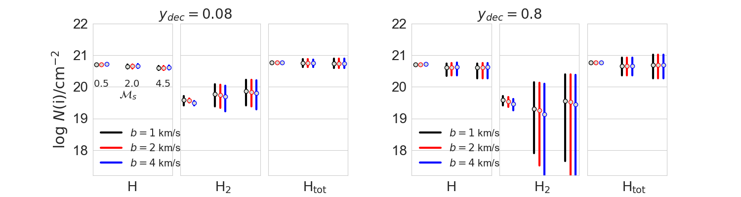
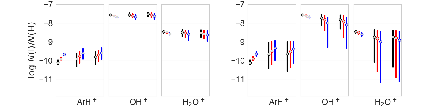
Figure 6.— The median (points) and the 68 percentile range (bars) of the column density abundance PDFs, for our entire simulation set, and assuming our fiducial $I_{\rm UV}$, $\zeta$ and $\langle n\rangle$ and $\langle A_{V}\rangle$. For each simulation, the three bars correspond to different Doppler broadenings, $b=1$, 2, 4 km/s.

Appendix B B. Dependence on the LoS orientation

The magnetic field in the simulations introduces a preferred direction (the $B$ field is initiated along the $y$ axis). In Fig. 7 we plot the PDF median and dispersion for all the species and for all the simulations considered here, for LoS parallel to $x$, $y$ or $z$. As evident from the figure, the results are weakly sensitive to the direction of the LoS.

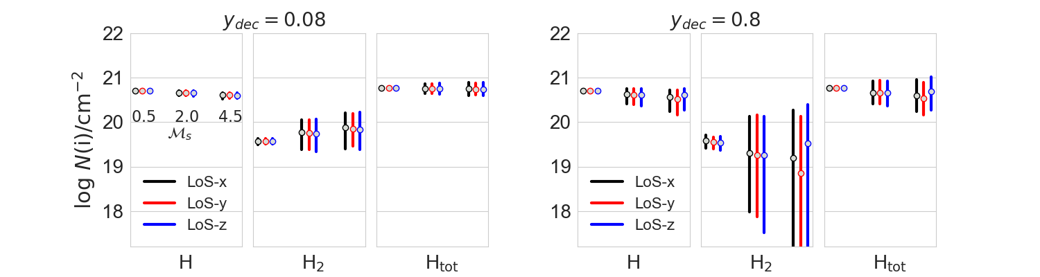
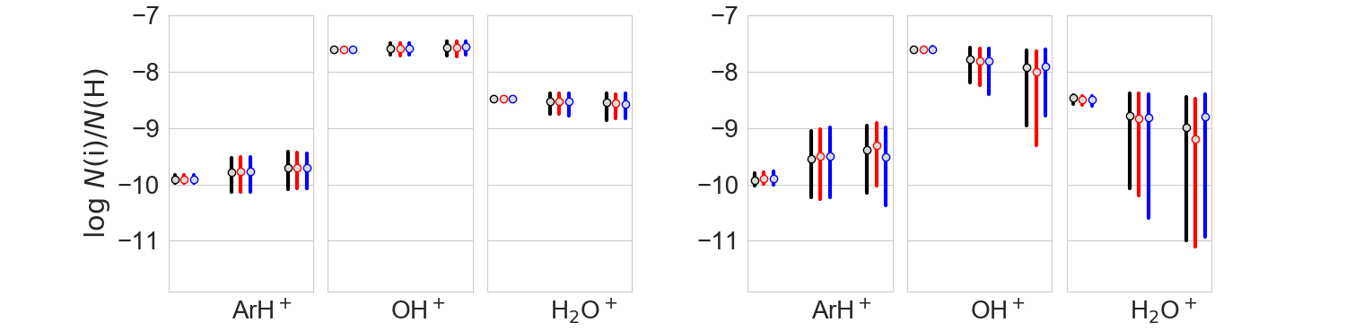
Figure 7.— The median (points) and the 68 percentile range (bars) of the column density abundance PDFs, for our entire simulation set, and assuming our fiducial $I_{\rm UV}$, $\zeta$ and $\langle n\rangle$ and $\langle A_{V}\rangle$, and $b=2$ km/s. For each simulation, the three bars correspond to different assumed orientations of the LoS: along $x$ (black), $y$ (red), and $z$ (blue). The $B$ field in the simulations is initialized along the $y$ axis.

References

- Arnold et al. (2015) Arnold, I., Thomas, E., Loch, S. D., Abdel-Naby, S., & Ballance, C. P. 2015, Journal of Physics B: Atomic, Molecular and Optical Physics, 48, 175005
- Audit & Hennebelle (2010) Audit, E., & Hennebelle, P. 2010, Astronomy and Astrophysics, 76, 1
- Bell et al. (2006) Bell, T. A., Roueff, E., Viti, S., & Williams, D. A. 2006, Monthly Notices of the Royal Astronomical Society, 371, 1865
- Bialy et al. (2017a) Bialy, S., Bihr, S., Beuther, H., Henning, T., & Sternberg, A. 2017a, The Astrophysical Journal, 835, 126
- Bialy et al. (2017b) Bialy, S., Burkhart, B., & Sternberg, A. 2017b, The Astrophysical Journal, 843, 92
- Bialy & Sternberg (2015) Bialy, S., & Sternberg, A. 2015, Monthly Notices of the Royal Astronomical Society, 450, 4424
- Bialy & Sternberg (2016) —. 2016, The Astrophysical Journal, 822, 83
- Bialy & Sternberg (2019) —. 2019, The Astrophysical Journal, 881, 160
- Bialy et al. (2015) Bialy, S., Sternberg, A., Lee, M.-Y., Petit, F. L., & Roueff, E. 2015, The Astrophysical Journal, 809, 122
- Burkhart et al. (2009) Burkhart, B., Falceta-Goncalves, D., Kowal, G., & Lazarian, A. 2009, The Astrophysical Journal, 693, 250
- Chepurnov et al. (2015) Chepurnov, A., Burkhart, B., Lazarian, A., & Stanimirovic, S. 2015, The Astrophysical Journal, 810, 33C
- Choi & Stone (2012) Choi, E., & Stone, J. M. 2012, Astrophysical Journal, 747
- Draine (1978) Draine, B. T. 1978, The Astrophysical Journal Supplement Series, 36, 595
- Draine & Bertoldi (1996) Draine, B. T., & Bertoldi, F. 1996, The Astrophysical Journal, 468, 269
- Federman et al. (1979) Federman, S. R., Glassgold, A. E., & Kwan, J. 1979, The Astrophysical Journal, 227, 466
- Federrath et al. (2008) Federrath, C., Klessen, R. S., & Schmidt, W. 2008, The Astrophysical Journal, 688, L79
- Field (1965) Field, G. B. 1965, The Astrophysical Journal, 142, 531
- Field et al. (1969) Field, G. B., Goldsmith, D. W., & Habing, H. J. 1969, The Astrophysical Journal, 155, L149
- Fischera & Dopita (2004) Fischera, J., & Dopita, M. A. 2004, The Astrophysical Journal, 611, 919
- Gazol & Kim (2013) Gazol, A., & Kim, J. 2013, The Astrophysical Journal, Volume 765, Issue 1, article id. 49, 8 pp. (2013)., 765
- Glassgold & Langer (1974) Glassgold, A. E., & Langer, W. D. 1974, The Astrophysical Journal, 193, 73
- Gnedin & Draine (2014) Gnedin, N. Y., & Draine, B. T. 2014, The Astrophysical Journal, 795, 37
- Heiles & Troland (2003) Heiles, C., & Troland, T. H. 2003, The Astrophysical Journal, 586, 1067
- Heyer et al. (2009) Heyer, M., Krawczyk, C., Duval, J., & Jackson, J. M. 2009, The Astrophysical Journal, 699, 1092
- Hill et al. (2008) Hill, A. S., Benjamin, R. A., Kowal, G., et al. 2008, The Astrophysical Journal, 686, 363
- Hollenbach et al. (2012) Hollenbach, D., Kaufman, M. J., Neufeld, D., Wolfire, M., & Goicoechea, J. R. 2012, The Astrophysical Journal, 754, 105
- Imara & Burkhart (2016) Imara, N., & Burkhart, B. 2016, The Astrophysical Journal, 829, 102
- Indriolo & McCall (2012) Indriolo, N., & McCall, B. J. 2012, The Astrophysical Journal, 745, 91
- Indriolo et al. (2015) Indriolo, N., Neufeld, D. A., Gerin, M., et al. 2015, The Astrophysical Journal, 800, 40
- Kaufman et al. (1999) Kaufman, M. J., Wolfire, M. G., Hollenbach, D. J., & Luhman, M. L. 1999, The Astrophysical Journal, 527, 795
- Kowal et al. (2007) Kowal, G., Lazarian, A., & Beresnyak, A. 2007, The Astrophysical Journal, 658, 423
- Le Petit et al. (2006) Le Petit, F., Nehme, C., Le Bourlot, J., et al. 2006, The Astrophysical Journal Supplement Series, 164, 506
- Lee et al. (2012) Lee, M.-Y., Stanimirović, S., Douglas, K. A., et al. 2012, The Astrophysical Journal, 748, 75
- McCourt et al. (2018) McCourt, M., Oh, S. P., O’Leary, R., & Madigan, A. M. 2018, Monthly Notices of the Royal Astronomical Society, 473, 5407
- McKee & Ostriker (2007) McKee, C. F., & Ostriker, E. C. 2007, Annual Review of Astronomy and Astrophysics, 45, 565
- Neufeld & Wolfire (2016) Neufeld, D. A., & Wolfire, M. G. 2016, The Astrophysical Journal, 826, 183
- Neufeld & Wolfire (2017) —. 2017, The Astrophysical Journal, 845, 163
- Piontek & Ostriker (2007) Piontek, R. A., & Ostriker, E. C. 2007, The Astrophysical Journal, 663, 183
- Röllig et al. (2006) Röllig, M., Ossenkopf, V., Jeyakumar, S., Stutzki, J., & Sternberg, A. 2006, Astronomy and Astrophysics, 451, 917
- Roman-Duval et al. (2010) Roman-Duval, J., Jackson, J. M., Heyer, M., Rathborne, J., & Simon, R. 2010, The Astrophysical Journal, 723, 492
- Sanchez et al. (2005) Sanchez, N., Alfaro, E. J., & Perez, E. 2005, The Astrophysical Journal, 625, 849
- Saury et al. (2014) Saury, E., Miville-Deschênes, M.-A., Hennebelle, P., Audit, E., & Schmidt, W. 2014, Astronomy & Astrophysics, 567, A16
- Schilke et al. (2014) Schilke, P., Neufeld, A., Müller, H. S. P., et al. 2014, Astronomy & Astrophysics, A29
- Sonnentrucker et al. (2015) Sonnentrucker, P., Wolfire, M., Neufeld, D. A., et al. 2015, The Astrophysical Journal, 806, 49
- Sternberg & Dalgarno (1995) Sternberg, A., & Dalgarno, A. 1995, The Astrophysical Journal Supplement Series, 99, 565
- Sternberg et al. (2014) Sternberg, A., Petit, F. L., Roueff, E., & Bourlot, J. L. 2014, The Astrophysical Journal Supplement Series, 790, 10S
- Stutzki et al. (1998) Stutzki, J., Bensch, F., Heithausen, A., Ossenkopf, V., & Zielinsky, M. 1998, Astronomy and Astrophysics, 336, 697
- Tielens & Hollenbach (2002) Tielens, A. G. G. M., & Hollenbach, D. 2002, The Astrophysical Journal, 291, 722
- Vazquez-Semadeni (1994) Vazquez-Semadeni, E. 1994, The Astrophysical Journal, 423, 681
- Vazquez‐Semadeni & Garcia (2001) Vazquez‐Semadeni, E., & Garcia, N. 2001, The Astrophysical Journal, 557, 727
- Walch et al. (2011) Walch, S., Wuensch, R., Burkert, A., Glover, S., & Whitworth, A. 2011, The Astrophysical Journal, 733, 47
- Waters & Proga (2019) Waters, T., & Proga, D. 2019, The Astrophysical Journal, 876, L3
- Winkel et al. (2017) Winkel, B., Wiesemeyer, H., Menten, K. M., et al. 2017, Astronomy & Astrophysics, 600, A2
- Wolfire et al. (1995) Wolfire, M., Hollenbach, D., McKee, C., Tielens, A., & Bakes, E. 1995, The Astrophysical Journal, 443, 152
- Wolfire et al. (2010) Wolfire, M. G., Hollenbach, D., & McKee, C. F. 2010, Astrophysical Journal, 716, 1191
- Wolfire et al. (2003) Wolfire, M. G., McKee, C. F., Hollenbach, D., & Tielens, A. G. G. M. 2003, The Astrophysical Journal, 587, 278