[figure]style=plain,subcapbesideposition=top
Bifurcating entanglement-renormalization group flows of fracton stabilizer models
Abstract
We investigate the entanglement-renormalization group flows of translation-invariant topological stabilizer models in three dimensions. Fracton models are observed to bifurcate under entanglement renormalization, generically returning at least one copy of the original model. Based on this behavior we formulate the notion of bifurcated equivalence for fracton phases, generalizing foliated fracton equivalence. The notion of quotient superselection sectors is also generalized accordingly. We calculate bifurcating entanglement-renormalization group flows for a wide range of examples and, based on those results, propose conjectures regarding the classification of translation-invariant topological stabilizer models in three dimensions.
The renormalization group (RG) is a ubiquitous concept throughout theoretical physics. Intuitively, real-space renormalization Wilson (1975) involves the rescaling of a system such that the short-distance correlations are integrated out. At the scale-invariant fixed points of an RG transformation, the system has either zero or infinite correlation length, corresponding to gapped or critical phases respectively. As such, RG serves as an important tool for the analysis of long-wavelength physics in a given theory.
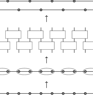
Since rescaling transformations increase the local Hilbert space dimension, conventional RG approaches have relied on truncating the local Hilbert space in a manner that does not affect long-range correlations. To further ensure that the long-range entanglement structure is preserved, which is particularly crucial for the classification and characterization of quantum matter, a more careful approach must be taken. A real-space renormalization procedure that exclusively removes short-range entanglement consists of applying local unitary circuits and projecting out degrees of freedom that have been completely disentangled into trivial states only Haah (2014). Along with the coarse-graining of degrees of freedom to rescale the system, such a procedure is referred to as Entanglement Renormalization (ER) Vidal (2007). Stable fixed points under ER are identified as representatives of quantum phases of matter. For many exactly solvable models with zero correlation length, ER can be implemented directly at the level of the Hamiltonian König et al. (2009); Aguado and Vidal (2008).
In this paper we apply ER to study the long-range entanglement structures of topological stabilizer models. In two dimensions, every translation-invariant topological stabilizer model is equivalent to copies of the 2D toric code Haah (2018); Bombin et al. (2012); Bombín (2014) and hence their classification is complete. The 2D toric code is a fixed point under ER. Hence, under ER, any 2D translation-invariant topological stabilizer model flows towards copies of the 2D toric code. In contrast, translation-invariant topological stabilizer models in three dimensions exhibit a rich variety of quantum phases due to the existence of fracton topological order Chamon (2005); Castelnovo et al. (2010); Bravyi et al. (2010); Castelnovo and Chamon (2012); Ma et al. (2017); Vijay et al. (2016); Williamson (2016); Vijay (2017); Vijay and Fu (2017); Slagle and Kim (2017); Halász et al. (2017); Devakul (2018a); Devakul et al. (2018a); Prem et al. (2019); Bulmash and Iadecola (2019); Song et al. (2019a); Brown and Williamson (2019); Weinstein et al. (2018); Hsieh and Halász (2017); Prem and Williamson (2019); Bulmash and Barkeshli (2019). While no systematic classification theorem or procedure has yet been established for these models, they can be organized into broad classes Dua et al. (2019a) based on the properties of their excitations and compactifications Dua et al. (2019b).
In Ref. Haah, 2014 it was found that Haah’s cubic code, the canonical example of a type-II fracton topological order with no string operators, bifurcates under ER. More precisely, under ER the cubic code splits into two decoupled models on a coarse-grained lattice: the original cubic code and cubic code B. The possibility of bifurcating ER was previously envisioned in Refs. Evenbly and Vidal, 2014a, b, c with the goal of describing critical states that violate the area law in two or more dimensions. Our goal is to extend the classification of topological phases in terms of ER fixed points to models that may bifurcate under ER. This approach faces an immediate conceptual hurdle: bifurcating models are not scale-invariant. In fact, under the conventional notion of quantum phase Chen et al. (2010), a bifurcating model defined on a lattice of spacing and the same model defined on a lattice of spacing belong to different phases of matter. Therefore one needs to revisit the definition of thermodynamic quantum phases under such circumstances.
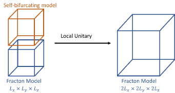
Fracton models are examples of bifurcating models. Under ER they may self-bifurcate or bifurcate into distinct models. Since self-bifurcating models give rise to an arbitrarily large number of copies of themselves under repeated ER, it is reasonable to consider them as free resources in the infrared limit. One can then formulate a generalized notion of fixed point where such free resources, i.e. the self-bifurcating models, are quotiented out. This generalizes the usual disentangling and projection steps in conventional ER where trivial product state degrees of freedom, which are the simplest example of a self-bifurcating state, serve as the free resource. The classification of bifurcating models via ER is then divided into two steps: first the classification of self-bifurcating fixed points and then the classification of quotient fixed points. The classification of self-bifurcating fixed points was previously studied from a resource oriented renormalization group perspective in Ref. Swingle and McGreevy, 2016a, b.
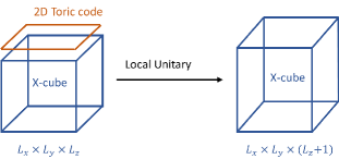
A similar point of view on fixed points of bifurcating ER has already played a key role in the understanding of foliated fracton models Shirley et al. (2019a, 2018a, 2018b, b, 2018c). The notion of foliated equivalence, local unitary equivalence up to adding stacks of 2D toric code, is rooted in the ER flow of foliated fracton models which produce stacks of 2D toric codes when they bifurcate. A stack of 2D toric codes is the simplest nontrivial self-bifurcating topological state in 3D. It is easy to see that it self-bifurcates under coarse-graining in the direction orthogonal to the toric code planes. The X-cube model is the canonical example with nontrivial foliated fracton order: under ER that coarse-grains by a factor of two along any axis it bifurcates, returning a copy of itself and a stack of 2D toric codes orthogonal to the axis. This reveals the X-cube model’s foliation structure and that it is a foliated fixed point, as it is foliated equivalent to itself after coarse-graining.
In this work, we propose to generalize the notion of foliated fracton equivalence to bifurcated equivalence which allows any self-bifurcating state as a resource, thus providing an equivalence relation that is relevant for all fracton models. We study the ER of a large range of fracton models, including 17 of Haah’s cubic codes Haah (2011) and all of Yoshida’s first-order fractal spin liquids Yoshida (2013), and find that they are all bifurcating fixed points. That is, under ER they either self-bifurcate, producing several identical copies, or they bifurcate into a copy of themselves along with some distinct models, referred to as B models. We demonstrate that the B models are self-bifurcating for all the examples considered. Our ER results are presented in table 1. Moreover, we find that the form of the B models is constrained by the mobilities of the topological quasi-particles in the original models. For instance, the presence of a planon in the original model causes a stack of 2D toric codes to appear amongst the B models. Such constraints on the B models motivate us to put forward several conjectures concerning the structure of 3D topological stabilizer models that have implications for their classification.
The paper is laid out as follows: in Sec. I.2, we introduce ER for gapped quantum phases of matter, discuss conventional and bifurcating ER fixed points, and define bifurcated equivalence and quotient superselection sectors. In Sec. II, we review Haah’s polynomial framework. In Sec. III, we explicitly identify bifurcating behavior in the ERG flows of a large range of models including 17 cubic codes Haah (2011) and all first-order fractal spin liquids Yoshida (2013). In Sec. IV, we discuss possible ERG flows for the distinct classes of topological order Dua et al. (2019a). In Sec. V, we study quotient superselection sectors in several examples. In the appendix, we provide numerical results for the number of encoded qubits for all models discussed, complimented by derivations of analytical expressions for a select few. We also present the ER for the X-cube model explicitly. The explicit ER process for all other models as listed is shown in the MATHEMATICA file SMERG.nb provided as supplementary material.
I Entanglement renormalization and phase equivalence
In this section we introduce the notions of quantum phase of matter and entanglement renormalization. We discuss how the definition of phase equivalence is informed by ERG fixed points. We then introduce the more general notion of bifurcated equivalence based upon bifurcating ERG fixed points. We also discuss how the notion of superselection sector is generalized to quotient superselection sector for bifurcating ERG fixed point models.
I.1 Gapped quantum phases of matter
Throughout the paper we consider lattice Hamiltonians in 3D with short-range interactions. We only consider translation-invariant Hamiltonians defined on cubic lattices.
A model is in a zero temperature gapped quantum phase if, in the energy spectrum, there is a finite gap between a nearly degenerate ground state subspace and the first excited state. Technically the energy gap must be uniformly lower bounded by a positive constant for a sequence of increasing system sizes approaching the thermodynamic limit Zeng et al. (2019). The energy splitting for the nearly degenerate ground state subspace must also vanish super-polynomially in the thermodynamic limit. The thermodynamic limit is approached as the ratio of system size to the lattice constant, or the short-distance cutoff length scale, goes to infinity . Two Hamiltonians are in the same phase if they are connected by a path of uniformly gapped Hamiltonians, possibly after adding in additional spins governed by the trivial paramagnetic Hamiltonian whose ground state is a product state. The addition of trivial degrees of freedom serves to stabilize the equivalence relation and allows for the comparison of models with a different number of spins per unit cell. In particular, models with the same but different can be meaningfully compared. Conversely, a quantum phase transition between gapped phases necessarily involves the gap closing.
The physical characteristics of zero temperature gapped phases can be studied via their ground states. Such ground states are in the same phase if and only if they are related by a quasi-adiabatic evolution Hastings and Wen (2005), possibly after stabilization by adding spins in a trivial product state. Constant-depth local unitary circuits are often used as a proxy for phase equivalence Chen et al. (2010), although strictly speaking they provide only a sufficient condition Haah et al. (2018). To compare bulk phase equivalence more generally one should consider stabilized (approximate) locality-preserving unitary maps, or quantum cellular automata. For dispersionless commuting projector Hamiltonians it appears sufficient to consider stabilized exact locality-preserving unitary maps, up to a change in the choice of local Hamiltonian terms that preserves the ground space and gap but may shift higher energy levels.
Throughout this work, topological orders are stable gapped quantum phases defined by a topological degeneracy on torus and characterized by the existence of nontrivial quasiparticles. This includes:
-
•
Topological quantum liquid phases, whose ground state degeneracies on the torus have a constant upper bound. It is widely believed that these phases can be described by topological quantum field theories (TQFT) at low energy. We will thus refer to topological orders belonging to class as TQFT phases.
-
•
Fracton phases whose ground state degeneracies do not have a constant upper bound. The low-energy behaviors of these phases are not described by any conventional TQFTs.
I.2 Entanglement renormalization transformations
We now describe ER transformations following the pioneering work Haah (2014). Given a gapped Hamiltonian, an ER transformation consists of the following steps:
-
1.
Coarse-grain the system by enlarging the unit cell by a factor .
-
2.
Apply local unitary transformations to the Hamiltonian to remove short-range entanglement.
-
3.
Project out local degrees of freedom that are completely disentangled into a trivial state.
The result is a new Hamiltonian in the same phase of matter, defined on the coarse-grained lattice.
In order to maintain a well-defined notion of phase throughout a renormalization procedure, we fix the ratio to be infinite by taking an infinite system size while successively coarse-graining a finite lattice constant by a factor . For a system of finite size, coarse-graining amounts to reducing the number of unit cells in the system. In the thermodynamic limit this remains true, as the ratio of the number of unit cells before and after coarse graining is equal to even though both numerator and denominator diverge.

Conventionally it is expected that ERG flows within a gapped phase carry models towards a representative fixed point model that is invariant under the ERG flow. We depict such a situation schematically in Fig. 1, which shows Hamiltonians flowing towards RG fixed points in two gapped phases. The set of stable ERG fixed points then suffice to classify the gapped phases.
We remark that under ER copies of the trivial Hamiltonian are produced at an exponential rate, as the trivial Hamiltonian in spatial dimensions splits into copies of itself under coarse-graining by a factor . Hence to find any fixed points we must mod out by this self-replicating trivial model. Furthermore, for an ERG fixed point model to lie in the same phase after a change of scale, the trivial Hamiltonian must also be modded out in the definition of phase. This is clearly a necessary condition for a definition of phase that does not rely on a choice of lattice scale, as is commonly desired.
Fixed point Hamiltonians under the form of ER we consider here must satisfy
| (1) |
for some finite-depth quantum circuit , where is the coarse-graining factor. The Hamiltonian has the same local terms as the original Hamiltonian , but the degrees of freedom sit on the sites of a coarse-grained lattice with spacing . The equivalence denotes equality up to the addition of disentangled spins governed by the trivial Hamiltonian to either side, and changing the choice of local Hamiltonian terms in a way that preserves the ground space. In particular, this implies that and are in the same phase. This relation holds for commuting projector Hamiltonians that describe TQFT phases Kitaev (2003); Levin and Wen (2005); Koenig et al. (2010); Walker and Wang (2012); Williamson and Wang (2017), and hence they are fixed points under ER König et al. (2009); Aguado and Vidal (2008). This allows the lattice scale to be ignored in the definition of TQFT phases.
I.3 Bifurcating entanglement renormalization and bifurcated equivalence
Models that are governed by conventional ERG fixed-point Hamiltonians with topological order fall into the category of TQFT phases. All known two-dimensional fixed-point models are of this type. However, in three dimensions, fracton models with topological order have been discovered that bifurcate under ER. This means that performing one step of ER on a model produces multiple nontrivial decoupled models. That is, for some finite-depth quantum circuit we have
| (2) |
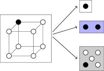
where is again the coarse-graining factor and is the number of nontrivial decoupled models, or branches. We remark that this decomposition into decoupled models may not be unique. An illustration of a bifurcating ER transformation is shown in Fig. 2.
A model is a bifurcating fixed point if any of the resulting models on the right hand side of Eq. (2) are equivalent to it, i.e. without loss of generality. In particular, all of the examples that appear in this work are bifurcating fixed points. Bifurcating fixed points can be either self-bifurcating fixed points or quotient fixed points which are defined as follows:
-
•
A model is a self-bifurcating fixed point with branching number if all of the resulting models on the right hand side of Eq. (2) are equivalent to it, i.e. for . For example, a self-bifurcating fixed point with branching number satisfies
(3) -
•
A bifurcating fixed point model is a quotient fixed point if the models for are self-bifurcating fixed points that are not equivalent to . More specifically we may refer to such an as a quotient fixed point with respect to the self-bifurcating Hamiltonian . An example of a quotient fixed point model, with respect to two decoupled self-bifurcating fixed points, is given by
(4) where and both satisfy Eq.(3).
[]
\sidesubfloat[]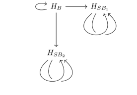
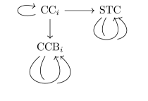
In Fig. 3, we represent the above self-bifurcating and quotient ERG fixed point examples using a diagrammatic notation. In our bifurcating ERG fixed point diagrams the models resulting from one step of ER, corresponding to the right hand side of Eq. (2), are found by following all arrows leaving a model, corresponding to the left hand side of Eq. (2). Such a diagram represents a generalized fixed point when all arrows leaving models in the diagram return to models within the diagram. This captures conventional fixed points, bifurcating fixed points and limit cycles, which can be removed by increasing the amount of coarse-graining performed during one step of ER. Further examples of bifurcating ERG fixed point models are presented in section III, with the results summarized in table 1. We remark that since Eq. (2) is not unique for a given Hamiltonian it is possible for a model to be a self-bifurcating fixed point under one ERG flow, and a quotient fixed point under another, see section III.3 for such an example.
In contrast to conventional ER fixed points, bifurcating ER fixed point Hamiltonians on different lattices are not in the same phase, i.e. is not phase equivalent to . This is evident from the presence of nontrivial models with on the right hand side of Eq. (2). For a self-bifurcating model, , that satisfies Eq.(3) with the reason for this inequivalence is especially clear: two copies of cannot be equivalent to a single copy unless is in the trivial phase. This is depicted in Fig. 4.

Self-bifurcating fixed point models produce copies of themselves at an exponential rate under ERG flow. This rate is given by the branching number, which obviously satisfies , but can be further shown to satisfy for states that satisfy an area law Haah (2014), which are the relevant ones in the study of gapped phases. This is analogous to the exponential splitting of trivial models in the ERG flow of a conventional fixed point model. Inspired by the modding out of trivial models in the definition of gapped phase equivalence, here we introduce the notion of bifurcated equivalence where all self-bifurcating models are modded out. More specifically, we write if stacked with some number of copies of lies in the same conventional phase as stacked with some number of copies of . This is bifurcated equivalence with respect to a self-bifurcating fixed point model . When is a trivial Hamiltonian we recover the conventional phase equivalence, when is a stack of 2D topological orders we recover foliated fracton equivalence. Similarly we write if stacked with copies of is equivalent to stacked with copies of . More generally we denote bifurcated equivalence by whenever there exist self-bifurcating models such that . See Fig. 10 (b) for a nontrivial example involving both foliated fracton equivalence and the more general bifurcated equivalence.
The bifurcated equivalence relation serves to essentially remove dependence on the lattice scale from the equivalence class of a quotient fixed point Hamiltonian since in that case. We remark that models may be bifurcated equivalent, even when they are not in the same conventional gapped phase. In particular any self-bifurcating model is in the trivial bifurcated equivalence class, even though the model may be in a nontrivial conventional phase. In Fig. 4 the dotted line denotes a conventional phase boundary, whereas the whole diagram lies in the same trivial bifurcated equivalence class. It is also useful to generalize the equivalence relation accordingly by allowing for stacking with arbitrary self-bifurcating models, which we denote . With this definition in hand the condition for a quotient fixed point resembles the conventional fixed point condition
| (5) |
I.4 (Quotient) superselection sectors
A nontrivial superselection sector on some region is an excitation that can be supported on but not created by any operator within a neighborhood of . Superselection sectors are equivalent if they are related by the application of an operator within a neighborhood of , or equivalently fusion with a local excitation in . Under ER excitations may split due to a change in the choice of local Hamiltonian terms allowed in the relation. This may create local excitations in the trivial Hamiltonians that are modded out by the relation. Hence for superselection sectors to be invariant under ER, local excitations must be modded out in their definition.
For the same reason, to define quotient superselection sectors (QSS) that are invariant under quotient ER we must mod out any excitations that can flow into a self-bifurcating fixed point model, as these models are modded out by the relation. Representatives of potential QSS are then given by the fixed point excitations under quotient ER. This captures the notion of QSS for foliated fracton models as a special case when the self-bifurcating model is taken to be a stack of 2D topological orders Shirley et al. (2018c).
II Entanglement renormalization in the polynomial framework
In this section we introduce translation-invariant stabilizer models, Clifford ER transformations and phase equivalence relations, along with their descriptions in the language of polynomial rings from commutative algebra.
II.1 Translation-invariant stabilizer models
Translation-invariant stabilizer Hamiltonians are specified by a choice of mutually commuting local Pauli stabilizer generators . The generators become the interaction terms in a Hamiltonian,
| (6) |
where are lattice vectors. In the above equation, indicates a local generator after translation by a lattice vector . The local generator is a tensor product of local Pauli operators acting on a set of qubits or qudits. Without loss of generality, we consider stabilizer models on a cubic lattice.
II.1.1 Clifford phase equivalence and entanglement renormalization
Maps between translation-invariant stabilizer Hamiltonians are given by locality-preserving Clifford operations, which map local Pauli operators to local Pauli operators. These Clifford operations include local Clifford circuits which are generated by CNOT, Phase and Hadamard gates, and nontrivial Clifford cellular automata, which are required to disentangle certain invertible phases Haah et al. (2018). In addition, locality-preserving automorphisms of the lattice, such as the redefinition of coordinates via modular transformations and coarse graining, are also included.
Phase equivalences of translation-invariant stabilizer Hamiltonians are given by locality-preserving Clifford operations up to stacking with trivial models.
For our Clifford ER transformations, we restrict to local Clifford circuits, coarse-graining, and discarding trivial models, as the modular transformations and other nontrivial locality-preserving operations can be moved to a single final step when comparing models. A change in the choice of local stabilizer generators that preserves the stabilizer group is also allowed when comparing two models, as in the relation above. As CNOT, Phase and Hadamard gates generate the Clifford group, they are sufficient to implement ER of Pauli stabilizer codes.
In 2D all translation-invariant topological stabilizer models were classified and shown to be equivalent, under locality-preserving Clifford operations, to copies of the 2D toric code. This implies that all translation-invariant topological stabilizer models in 2D flow to ER fixed points. Conversely in 3D examples of translation-invariant topological stabilizer models that bifurcate under ER are known, and the classification problem remains completely open, due to the existence of fracton models. Our goal is to study the bifurcating ERG flows of known fracton stabilizer models to gain clues about the 3D classification problem.
The examples considered in this work are all in CSS form Calderbank and Shor (1996); Steane (1996), which should be preserved under ER, hence we have found it sufficient to consider Clifford circuits that consist of CNOT gates alone. In particular, the unitaries used in the ER of our examples are given by Clifford circuits where is finite and each layer of gates is a translation-invariant tensor product of CNOT gates.
II.2 The polynomial framework
Translation-invariant stabilizer Hamiltonians can be conveniently expressed in terms of polynomials. The use of a polynomial description in a similar context dates back to work on classical cyclic codes Imai (1977); MacWilliams and Sloane (1977); Güneri and Özbudak (2008). The polynomial approach for quantum codes on a lattice was primarily developed by Haah. Interested readers are directed to Ref. Haah, 2013a for further details. We proceed by introducing several definitions from the polynomial language that are necessary and sufficient to describe ER. These definitions are demonstrated via examples.
II.2.1 The stabilizer map
For a stabilizer model on a cubic lattice, the stabilizer generators supported on a cubic unit cell can be expressed in terms of the position labels of the vertices on the cube as shown below
| (16) |
The canonical example of a type-II model is Haah’s code, or cubic code 1, which has the following stabilizer generators
| (34) |
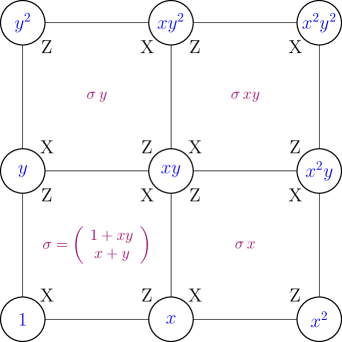
In the -stabilizer generator, the sites on which the first qubit is acted upon by the Pauli operator are at positions , , and of the unit cell. We take this set of positions and write a polynomial corresponding to this set . Similarly, the polynomial corresponding to the action of the Pauli operator on the second qubit on vertices in the unit cell is . The polynomials corresponding to the action of the operator on the first and second qubits on each site involved in the -stabilizer generator are given by and . These polynomials refer to exponents of Pauli operators, and hence the addition of polynomials corresponds to the multiplication of operators. One can consider this polynomial representation to be a map from the position labels to the set of Pauli operators. This map is called the stabilizer map which can be written as a matrix where is the number of qubits on each vertex in the unit cell and is the number of stabilizer generators per unit cell in the translation-invariant Hamiltonian. In such a matrix, each column represents a term in the Hamiltonian and all translates of these terms can be generated by acting on the column by multiplication with monomials of translation variables. We illustrate the polynomial representation for a non-CSS model using the example of Wen’s plaquette model in Fig. 5.
In this paper, we focus on CSS models for which the stabilizer map takes the form
| (37) |
where is the map for the -sector. Each column, labeled , specifies a stabilizer generator. The rows of the block are labeled (), where the row index is the index of the qubit in the unit cell. For example, the stabilizer map for cubic code 1 is
| (42) |
We remark that all stabilizers of the model can be generated by the action of the stabilizer map on a column of translation variables. The translation action can be expressed in terms of the position variables . For example, the -stabilizer on the unit cell at position relative to the origin is denoted
| (47) |
Using this, or any other translation of the -stabilizer generator in Eq (42) lead to the same Hamiltonian. Hence, multiplying columns by monomials results in an equivalent stabilizer map. For example, we could divide the second column of the cubic code stabilizer map by , corresponding to a unit translation in the negative direction along each axis. The resulting equivalent stabilizer map can be written as
| (52) |
where we have introduced the inverse variables and which satisfy , and . In the terminology of commutative algebra, introducing negative powers for translation variables involves going from a polynomial ring to a Laurent polynomial ring.
II.2.2 Entanglement renormalization in the polynomial language
As discussed above, in the Clifford ER procedure after coarse-graining certain operations are allowed. These operations consist of acting on the stabilizer generators with Clifford gates, changing the choice of generators for the same stabilizer group and shifting the lattice sites. In the polynomial language, these operations are represented by matrices acting on the stabilizer map, from the left for Clifford gates and qubit shifts, and from the right for the shifting and redefinition of stabilizer generators. These operations were described in Ref. Haah, 2014. As our focus is on CSS models, we restrict our discussion to Clifford circuits made up of CNOT gates. In which case the action of ER operations on the stabilizer map are as follows:
-
•
Row operations
-
–
Elementary row operations:
An elementary row operation on a stabilizer map with rows is specified by two row indices and a monomial and acts as follows in the -sector,(53) This operation corresponds to a translation-invariant implementation of CNOT gates between the target qubits specified by and with the control qubits specified by . The corresponding action in the -sector is given by
(54) -
–
Row multiplication by a monomial:
Multiplying any of the rows in the stabilizer map by a monomial corresponds to shifting those qubits in some direction. For the polynomial entries , in a row specified by constant , the transformation is allowed, for any finite integers .
-
–
-
•
Column operations
-
–
Elementary column operations:
An elementary column operation on a stabilizer map with columns is specified by two column indices and a monomial and acts as follows:(55) This changes the choice of stabilizer generators by replacing those corresponding to by products of themselves with translates of the generator corresponding to . Such a change of choice of generators results in a phase equivalent Hamiltonian with the same ground space and shifted excitation energy levels.
-
–
Column multiplication by a monomial:
This corresponds to changing the choice of a stabilizer generator, translating it by a monomial. This has no effect on the Hamiltonian described by the stabilizer map, as it already includes all translations of the generators. For example, we used such a transformation above to modify the polynomial representation for the -stabilizer term of the cubic code to go from Eq. (42) to Eq. (52).
-
–
II.2.3 Modular transformations
The Clifford ER process only involves equivalences between models generated by coarse-graining, local Clifford gates, shifting the lattice sites and changing the choice of column generators. More generally modular transformations, which are locality-preserving automorphisms of the cubic lattice including shear transformations, preserve the bulk properties of a model. Hence, when deciding phase equivalence, modular transformations need to be taken into account. Formally, they correspond to the redefinition of translation variables to , where for are monomials in the translation variables that induce a bijection of the lattice sites.
Modular transformations are not used during the ER process. However, they are used when checking the equivalence of models that result from ER. We have also used them to find equivalences between some of the cubic codes. For example, cubic code 5 is related to cubic code 9 (and cubic code 15 is related to cubic code 16) via a modular transformation and hence they are in the same phase Dua et al. (2019a).
II.2.4 The excitation map
The excitations created by the action of a Pauli operator can be found by applying the excitation map to the polynomial representation of that Pauli operator. The map is expressed in terms of the stabilizer map via
| where | (58) |
is the symplectic matrix and denotes the identity matrix. The rows in the excitation map correspond to excitations of different stabilizer generators. The operators that do not excite translations of a particular generator correspond to columns that give 0 when acted upon by the corresponding row of . For example, one can see from that no stabilizer generators are excited by the action of a Pauli operator, as expected. More generally, the kernel of contains the operators that commute with all local Hamiltonian terms. In particular, the condition that the Hamiltonian terms themselves commute can be recast as , i.e. . This containment is saturated, , for infinite boundary conditions if and only if the Hamiltonian described by is topologically ordered Haah (2013a, b). Since consists of operators of finite extent in the polynomial formalism, implies that any operator that commutes with the Hamiltonian is in the span of the stabilizer group and so can be written as a sum of products of generators. This implies that any local operator must act as the identity on the degenerate ground space of the Hamiltonian with periodic boundary conditions, up to a proportionality constant that may be 0.
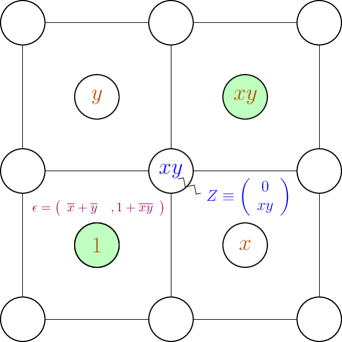
In Fig. 6, we depict how the excitation map gives the positions of excited stabilizers due to the action of a local operator on a qubit at position in the Wen-plaquette model. Another phase equivalent example is the toric code whose stabilizer map is given by
| (63) |
and whose excitation map is given by
| (66) |
Considering the action of a local operator on the first qubit at position . The action of this local operator is represented by the following column
| (71) |
and the action of the excitation map on this operator gives
| (74) |
This implies that the stabilizers at positions and are excited due to the action of on toric code. Similarly as for the polynomial description of Pauli operators, addition of excitation polynomials corresponds to fusion of excitations.
The image of the excitation map contains topologically trivial configurations of excitations. For cubic code stabilizer maps, which take the following form
| (79) |
The excitation map is given by
| (82) |
For any CSS model, the and the generator excitation sectors are decoupled, and in the case of the cubic codes they are related by a spatial inversion transformation. For cubic codes, the polynomials in the image of the excitation map for generators belong to the idealaaaAn ideal of a polynomial ring contains elements such that for all and all . generated by and i.e. where and are arbitrary polynomials with coefficients. We refer to this ideal, , as the stabilizer ideal Haah (2013a).
II.2.5 Coarse-graining the stabilizer and excitation maps
Coarse-graining by a factor of 2 enlarges the unit cell by the same factor. Hence, after coarse-graining, the original translation variables , and are transformed to , and on the new lattice. Suppose coarse-graining by a factor of 2 in the -direction is performed, i.e. . The coarse-grained unit cell has double the number of qubits and stabilizer generators. This coarse-graining transformation is implemented by the transformation of the original translation variables
| (89) |
where is a new translation variable. For example, this coarse-graining sends the stabilizer map of the 2D toric code from Eq. (63) to
| (98) |
It is shown below that after the application of local CNOT gates, column operations and the removal of qubits in the trivial state, the original stabilizer map is recovered.
The coarse-grained excitation map is defined in terms of the coarse-grained stabilizer map via .
II.2.6 Coarse-graining factor and trivial charge configurations
For the qubit-stabilizer models studied in this paper, we consider coarse-graining by factors of , i.e. . It was shown in Ref. Haah, 2013b, 2014 for cubic code 1 that the set of trivial charge configurations referred to as the annihilator of the charge module Haah (2013b), denoted , shows self-reproducing behavior under coarse-graining by a factor of 2. The annihilator of the cubic code 1, , is given by the ideal . Here, for example, specifies a trivial charge configuration with the stabilizers excited at positions , , and under the action of a local operator. After coarse-graining, the annihilator is given by in terms of the coarse-grained variables and hence has the same form as . This suggests that cubic code 1 renormalizes into a model similar to itself. In fact, the annihilators of the charge modules for the two codes that are extracted after ER of cubic code 1 i.e. itself and cubic code 1B, are exactly the same. We find this self-reproducing behavior for all the cubic codes and the corresponding B models; the form of the annihilator after coarse-graining by a factor of 2, retains the original form as just like in the case of cubic code 1. Conversely, under coarse-graining by a factor of 3, the annihilator does not retain the original form. For any self-bifurcating fixed point model, it obviously follows that the models extracted after ER retain the same annihilator. For the bifurcating quotient fixed point models, which split into a copy of themselves and some B models under ER, having the same form of annihilator after coarse-graining implies that the annihilators of the B models contain the original annihilator .
| Model | Particle mobilities | Type | ER | ER of the B models | QSS group |
|---|---|---|---|---|---|
| 3DTC | 3 | TQFT | 3DTC | ||
| X-cube | 0,1,2 | foliated type-I | X-cube+STC | STC+STC | |
| CC1 | 0 | type-II | CC1+ | + | |
| CC2,3,4,7,8,10 | 0 | type-II | CCi+CCi | 0 | |
| CC5,6,9 | 0,1 | fractal type-I | CCi+CCi | 0 | |
| CCbbbThe ER results shown require an initial coarse-graining step for CC13 and CC17.,d | 0,1,2 | fractal type-I | CCi++STC | + | cccThis QSS was calculated for in Sec. V.0.3. The QSS of can be calculated similarly. |
| CC14dddCC14 shows both self-bifurcating and bifurcating ERG behavior | 0,1,2 | fractal type-I | CC14+CC14 | 0 | |
| First-order FSL | model dependent | model dependent | FSL+FSL | 0 |
III Examples of bifurcating entanglement renormalization
In this section, we find bifurcating ERG flows for explicit examples of fracton models. Some of the fracton models treated are found to be self-bifurcating fixed points while others are quotient bifurcating fixed points. Moreover, we find that some models may admit several qualitatively different ERG flows. We give such an example that is either a self-bifurcating fixed point or a quotient bifurcating fixed point, depending on the ER transformation chosen.
The models we consider include several examples with known ERG flows: the 3D toric code (3DTC), a stack of 2D toric codes along an axis (STC), the X-cube model (X-cube), and Haah’s cubic codes 1 () and 1B (). Beyond these known examples we also find the ERG flows of the 16 other CSS cubic codes Haah (2011, 2013b) 2-17 () and the B codes thus produced (CCB), as well as all first-order fractal spin liquids Yoshida (2013) (FSL), a simple example of which is the Sierpinski fractal spin liquid Castelnovo and Chamon (2012) (SFSL). In the next section we put the ERG flows found for these examples into context by organizing them according to the type of 3D topological order each model displays Dua et al. (2019a).
We have followed a simple heuristic to find ER transformations for the example models listed in table 1. We outline this process in appendix B, and apply it to the X-cube model as a demonstrative example.
III.1 Self-bifurcating fixed points
[]
\sidesubfloat[]
\sidesubfloat[]
\sidesubfloat[]
The coarse-graining step of the ER procedure can involve one, two or all three lattice directions. Self-bifurcating models can be divided into three categories according to the minimal number of directions one must coarse-grain for the model to bifurcate. Sorting the self-bifurcating models in this way is convenient when it comes to organizing them according to the type of topological order they exhibit, as discussed in next section.
An important necessary condition for self-bifurcation with is that the number of encoded qubits under periodic boundary conditions doubles when the number of sites along each axis is doubled. This is because a self-bifurcating model with on a lattice with sites along each axis splits into two copies of itself when coarse grained by a factor of 2, each of which lives on a decoupled lattice with sites.
We discuss examples of stabilizer models that we have found to self-bifurcate under ER below. Examples of self-bifurcating models and their ERG flows are depicted in Fig. 7 using our diagrammatic notation for bifurcating ERG fixed points.
III.1.1 A stack of 2D toric codes
The stabilizer map for a stack of 2D toric codes along the direction, parallel to the plane, appears identical to that in Eq. (63). After coarse-graining in the direction the stabilizer map is identical to that in Eq. (98). Applying a row operation
to the coarse-grained stabilizer matrix from Eq. (98) results in
| (107) | ||||
| (116) |
After performing additional row operations CNOT, CNOT, CNOT and column operations Col and Col, the model becomes
| (125) |
which is nothing but a stack of 2D toric codes and two qubits per site in a product state. Hence, the stack of toric codes along the axis is a fixed point under ER in . The stack of 2D toric codes stabilizer map in Eq. (63) has symmetry up to relabeling of the qubits. Hence, it is also a fixed point under ER in . Furthermore, for the stack of 2D toric codes along the direction, we can trivially coarse-grain the stabilizer map along by taking
| (130) |
as does not enter the stabilizer map. This simply results in two decoupled copies of the stack of 2D toric codes Hamiltonian. Hence, a stack of 2D toric codes is self-bifurcating under ER. This provides an example of a model that self-bifurcates after ER in only one direction and is a fixed point under ER along either of the orthogonal directions.
III.1.2 Yoshida’s fractal spin liquids
We now move on to show that a far more interesting class of examples, the first-order fractal spin liquids of Yoshida Yoshida (2013), are all self-bifurcating under ER. The general form of the stabilizer map for these models is
| (131) |
where and are polynomials in the single translation variable . Such a model is type-II if and only if and are not algebraically related Yoshida (2013). This class of models also contains fractal type-I lineon models for , , stacks of 2D toric code for , stacks of 2D fractal subsystem symmetry-protected models Devakul et al. (2018b); Devakul and Williamson (2018); Stephen et al. (2018); Devakul (2018b); Daniel et al. (2019) for , , and decoupled 1D cluster states for , . We remark that and can be exchanged in the above models up to a redefinition of the lattice and an on-site qubit swap.
Under coarse-graining along :
| (138) |
where is the translation variable on the coarse-grained lattice, the stabilizer map becomes
| (139) |
Applying row operations: CNOT, CNOT, CNOT and column operations Col, Col leads to the stabilizer map
| (140) |
The first and third qubits are disentangled in the above stabilizer map and hence can be removedeeeUp until this step, the same ER process as shown works if is generalized to , along with a similar generalization for .. The resulting stabilizer map is
| (141) |
which is also a first-order FSL, where has been replaced by . We now notice that due to the symmetry between and in a first-order FSL one can apply essentially the same ER transformation, this time coarse-graining , so that is replaced by . For a polynomial over , a useful property is that . This leaves only functions of in the coarse-grained stabilizer map, so we coarse-grain again, along this time, sending
| (142) |
This results in the stabilizer map splitting into two copies of the original model, and hence all qubit first-order FSL models are self-bifurcating fixed points with . This includes the stack of 2D toric codes for and the trivial model for . Furthermore, if then and the model is a conventional fixed point under ER that coarse-grains along only, while being a self-bifurcating fixed point under ER that coarse-grains both and , and similarly if and are swapped.
A particular example, the SFSL model, is obtained when , , this model has a fractal logical operator in the plane and a lineon operator along Yoshida (2013). Our results indicate that the model is invariant under ER along the direction of the string operator and self-bifurcates under ER in the plane of the fractal operator.
The above ER transformations were essentially based on the observation that the 2D first-order fractal subsystem symmetry breaking (classical) spin models, from which the first-order FSLs are built, are self-bifurcating under ER. This can easily be seen by following the ER transformation of the FSL before Eq. (141) with the second qubit and generator, as well as the coordinate, dropped from the stabilizer map. This connection generalizes straightforwardly to provide ER transformations for 3D FSLs based upon self-bifurcating 2D fractal subsystem symmetry breaking spin models that may not be first-order. We remark that higher-order FSLs need not be self-bifurcating, as cubic code 1, which is not self-bifurcating, is equivalent to a second-order FSL Yoshida (2013). FSL forms for this, and some other cubic codes are presented in appendix C. The explicit mapping transformations can be found in the supplementary MATHEMATICA file SMERG.nb. An interesting open problem is the classification and characterization of higher-order self-bifurcating 2D fractal subsystem symmetry breaking spin models and the 3D FSLs built from them Shirley et al. (2019c).
We remark that a form of real-space RG was considered for the FSLs in Ref. Yoshida, 2013, however it does not conform to the strict definition of ER used here, where the phase of matter cannot change. Instead, degrees of freedom that were not fully disentangled were projected out, which is capable of changing the phase by projecting out an arbitrary nontrivial decoupled model. Our ER results are consistent with the RG results in Ref. Yoshida, 2013.
For the details of the ER procedures for the other examples discussed below, we refer the reader to the MATHEMATICA file SMERG.nb in the Supplementary Material.
III.1.3 Cubic codes 5, 6 and 9
III.1.4 Cubic codes 2–4, 7, 8 and 10
These cubic codes are not fixed points under ER along any single lattice directions, and self-bifurcate only after doing ER along all three lattice directions together, see Fig 7 (c). This is consistent with them being either fractal type-I, or type-II, fracton models Dua et al. (2019a).

III.2 Quotient bifurcating fixed points
A quotient bifurcating fixed point is defined by its branching under ER into a copy of itself and an inequivalent self-bifurcating model, which may consist of several decoupled self-bifurcating models. Verifying the inequivalence of models can be quite subtle, as it requires one to consider arbitrary locality-preserving unitaries, including coarse graining and modular transformations. Ref. Haah, 2014 introduced an approach to proving the inequivalence of models based upon the behavior of their ground space degeneracies. In particular, the following sufficient condition was proposed to confirm that a model could not be a self-bifurcating fixed point
| (143) |
for integers . Where is the number of encoded qubits in the ground space on an system with periodic boundary conditions. This is in contrast with the necessary condition that in Eq. (143) for any self-bifurcating model.
III.2.1 Cubic code 1
It was shown in Ref. Haah, 2014 that CC1 bifurcates into a copy of itself and an inequivalent model CCB1 under ER and hence is a quotient fixed point, see Fig. 8. To prove this inequivalence the scaling of the number of encoded qubits in the ground space, , was used. This scaling can be directly inferred from the following formula for CC1 Haah (2013b, 2014, a)
| (144) |
Thus, any model equivalent to CC1 cannot self-bifurcate. Since was demonstrated to be a self-bifurcating model, and CCB1 cannot be in the same phase.
III.2.2 Cubic codes 11-17
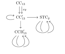
We have found that these cubic codes are quotient fixed points under ER. CCi, for , branches into a copy of CCi, a stack of 2D toric codes along one direction and a self-bifurcating model CCBi, see Fig. 9. This is consistent with these models being fractal type-I topological orders that support planons. See Appendix D of Ref. Dua et al., 2019a for a description of these planons. For CC13 and CC17 the quotient fixed point behavior occurs after an initial step of coarse-graining, see Fig. 10.
[]
\sidesubfloat[]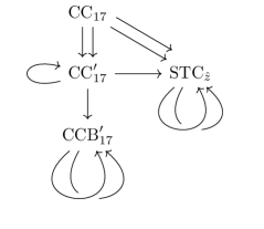
\sidesubfloat[]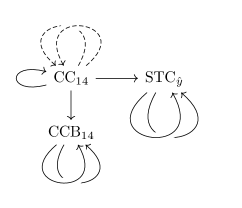
III.3 Quotient bifurcating and self-bifurcating fixed point behavior for cubic code 14
We have found two distinct ERG flows for CC14: under one ER procedure CC14 is self-bifurcating with . Under another ER procedure CC14 appears to be a quotient fixed point as it bifurcates into a copy of itself, a stack of 2D toric codes and another self-bifurcating model CCB14, see Fig. 10. Due to the absence of any correction factor in Eq. (143) for CC14, as it is a self-bifurcating fixed point, the standard method to argue for inequivalence to CCB14 and a stack of 2D toric codes does not apply. On the other hand, we have been unable to find a direct equivalence between CC14 and CCB14 plus a stack of 2D toric codes. It is clear from the ERG flows that two copies of CC14 is phase equivalent to CC14, CCB14 and a stack of toric codes. Thus in the case that the ERG flows are inequivalent, this would provide an interesting example of a phase equivalence that is catalyzed by the addition of a copy of CC14. In any case, all of the aforementioned models are in the same trivial bifurcated equivalence class.
This example raises the interesting question of whether all ERG flows for which a model is a bifurcating fixed point are equivalent. We remark that this is trivially true for conventional fixed points but requires a careful definition of equivalence for more general bifurcating ERG flows.
IV Entanglement renormalization in different types of 3D topological phases
In the recent fracton literature Dua et al. (2019a) 3D topological stabilizer models have been coarsely organized into four qualitatively distinct classes: TQFT, foliated and fractal type-I, and type-II topological orders. In this section we describe the salient features of these different classes, which are determined by the mobilities of their topological quasiparticles, and discuss the influence they have on possible ERG flows.
IV.1 TQFT topological order
TQFT topological order is characterized by a constant topological ground space degeneracy as the system size increases and deformable logical operators. In two dimensions, there is essentially only one type of translation-invariant topological stabilizer model, the 2D toric code which is described by a TQFT at low energy. This is due to a structure theorem Haah et al. (2018); Haah (2016) stating that any translation-invariant topological stabilizer model is equivalent under locality-preserving unitary to copies of the toric code and some disentangled trivial qubits.
Hence all TQFT stabilizer models in 2D are fixed points under ER, equivalent to a number of copies of 2D toric code. We expect similar behavior in 3D, that all TQFT stabilizer models are fixed points under ER equivalent to a number of copies of 3D toric code and hence are described by a TQFT at low energies, although this remains to be shown.
In 3D the logical operator pairs of the toric code are composed of deformable string and membrane operators. More general 3D translation-invariant topological stabilizer models that have a constant ground space degeneracy as system size increases, and so are TQFT topological orders, have been shown to resemble this behavior as their logical operators also come in string-membrane pairs Yoshida (2011). We conjecture that a stronger structure theorem holds for such models in three dimensions: i.e. a TQFT stabilizer model in 3D is locality-preserving unitary equivalent to copies of the 3D toric code (possibly with fermionic point particle Levin and Wen (2003); Walker and Wang (2012)), and disentangled trivial qubits.
IV.2 Type-I fracton topological order
Type-I fracton topological order is characterized by a sub-extensive ground space degeneracy and rigid string operators, which correspond to excitations with sub-dimensional mobilities. This type of topological order is divided into two broad categories which we treat separately below.
IV.2.1 Foliated type-I topological order
Foliated topological order is characterized via a foliation structure Shirley et al. (2018b, a); Slagle et al. (2019). Such models can be grown by adding layers of a 2D topological order, such as the 2D toric code, according to the foliation structure. The most studied example of this type is the X-cube model which can be grown by adding layers of 2D toric code as shown in Fig. 12. More formally, two Hamiltonians are foliated equivalent Shirley et al. (2019b) if they are connected by adiabatic evolution and addition of layers of two dimensional gapped Hamiltonians. When translation invariance is enforced, foliated equivalence is the same as bifurcated equivalence with respect to stacks of 2D topological orders. Foliated stabilizer models can have topological quasiparticles with a hierarchy of mobilities such as fractons, lineons and planons. Given their foliation structure in terms of 2D toric codes, they must always support planons. In fact, the X-cube model has planons in all the three lattice directions due to its foliation structure that allows layering with 2D toric code in the three lattice directions. Due to the underlying foliation structure of this class of models, the ground space degeneracy scales exponentially with the size of the system.
The canonical self-bifurcating example within this class of models is the stack of 2D toric codes. This serves as the B model for X-cube, which is a quotient fixed point that bifurcates into a copy of itself and a stack of 2D toric codes along each axis. This is a consequence of the fact that X-cube supports planons in all the three lattice planes. The ER process for X-cube in the polynomial language is presented in appendix B.
Since all 2D topological stabilizer model are essentially copies of 2D toric code, we expect that stacks of 2D toric code are the only self-bifurcating stabilizer models in the foliated class. Furthermore, we expect that all nontrivial foliated stabilizer models flow to quotient fixed points with stacks of 2D toric code serving as the B models. An interesting open question is whether all such quotient fixed point foliated stabilizer models are foliated equivalent to a suitably generalized X-cube model which is allowed to take on different foliation structures Shirley et al. (2018c, b, 2019b); Wang et al. (2019).
IV.2.2 Fractal type-I topological order
Fractal type-I topological order captures type-I models that support fractal logical operators and symmetries, due to which no foliation structure in terms of 2D Hamiltonians is known or likely possible. In fact, these models need not support planons at all. Due to the underlying fractal symmetry of this class of models, the ground space degeneracy fluctuates with the system size. The simplest example of this type of model is the Sierpinski fractal spin liquid model Yoshida (2013); Castelnovo and Chamon (2012) which supports two dimensional fractal operators in the plane along with rigid string operators in the direction as all particles in the model are lineons. This model was mentioned above as a special case of Yoshida’s first-order FSLs which were shown to be self-bifurcating. As expected, this model is invariant under ER along the direction alone but self-bifurcates under ER in the plane or for all the three directions at once.
There are also fractal type-I models amongst the cubic codes, some of which support fractons along with lineons and planons. We discuss the ER of two such examples below. The first is CC6 which is self-bifurcating and the other one is CC11 which is a quotient bifurcating fixed point:
CC6 is a self-bifurcating fixed point under ER that coarse-grains all three lattice directions together. One can perform a modular transformation on the stabilizer map of CC6 to bring the lineon string operator along a lattice direction. The transformed model is invariant under ER that coarse grains in the direction of the string operator, while it self-bifurcates under ER that coarse grains the directions orthogonal to it. The number of encoded qubits of CC6 is given by
This obeys
which implies that the number of encoded qubits always doubles upon doubling the system size. This is indeed consistent with the self-bifurcating behavior.
CC11 is an important fractal type-I example as it supports topological quasiparticles of sub-dimensional mobilities 0, 1 and 2. Performing ER that coarse-grains all the three directions together causes CC11 to bifurcate into a copy of itself, a lineon model CCB11, and a stack of 2D toric codes along . We conjecture that this bifurcating behavior is directly related to the mobilities of topological quasiparticles in CC11. The presence of planons in the planes leads to the extraction of a stack of toric codes parallel to planes. Similarly, a subset of lineons from the original model CC11 flow into the lineon model under ER. In fact, for each of the cubic codes 11–17, except cubic code 14, there is an ER procedure that leads to a self-bifurcating lineon B model. For CC14, we find a self-bifurcating fracton B model CCB14 which supports a composite lineon as mentioned in Table 3 of the appendix. For , the scaling of the number of encoded qubits with the system size, derived in the appendix, is found to be consistent with the self-bifurcating behavior.
On the other hand, we have found that the number of encoded qubits for CC11 is given by
Using this result, we notice that there exists an infinite family of system sizes for which the scaling of number of encoded qubits has a correction factor: for , we have
| (145) |
The argument from Ref. Haah, 2014 can then be used to show that the correction factor of cannot be eliminated for any choice of coarse-graining of the original model. Hence, CC11 cannot self-bifurcate and is therefore inequivalent to CCB11.
Numerical results for the number of encoded qubits in the ground space of CC indicate that such an inconsistency with self-bifurcating behavior may hold for all codes except CC14 for which the numerics are consistent with . In fact, as mentioned before, we show explicitly that there are two ERG flows for CC14, one in which it self-bifurcates and the other in which it splits into a copy of itself, a B model and a stack of 2D toric codes. The ER of CC14 is shown in Fig. 10 (c).
IV.3 Type-II topological order
Type-II topological order is defined by the absence of any logical string operators and characterized by a sub-extensive ground space degeneracy that fluctuates with the system size. For the models in this class, none of the elementary topological excitations or their nontrivial composites are mobile. In the previous section we discussed the canonical example from this class, cubic code 1, which is known to be a quotient fixed point. CC1 supports a fractal operator that moves excitations apart in three dimensions. We show in the MATHEMATICA file SMERG.nb that the other type-II cubic code modelsfffCC were rigorously proven to be type-II in Ref. Haah (2011) while CC7, CC8 and CC10 were found to be type-II according to the methods in Ref. Dua et al. (2019a).: CC, CC7, CC8, CC10 and a type-II first-order quantum FSL Yoshida (2013) are self-bifurcating fixed points.
V Quotient Superselection sectors
In this section we explore the flow of excitations under ER. We find the set of quotient superselection sectors for several quotient fixed point models by calculating their fixed point excitations under quotient ERG flow.
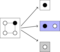
To find fixed point excitations under a quotient ERG flow it is important to understand how excitations split during each step of ER. The local unitaries performed as part of the ER process alter the form of stabilizer generators but do not cause any splitting. It is the redefinition of the stabilizer generators allowed by the equivalence relation during ER that determines how an excitation splits. This is illustrated in Fig. 13. In the polynomial description of ER, this redefinition is captured by column operations on the stabilizer map. A representation of the excitation splitting map can be found by taking the transpose of the matrix representation of the composition of all column operations involved in an ER transformation. For CSS models is block-diagonal and can be decomposed into separate maps and for the and sectors, respectively.
Quotient superselection sectors are defined to be equivalence classes of superselection sectors modulo any sectors that can flow into a self-bifurcating model. For stabilizer models the QSS form an abelian group under fusion. Nontrivial QSS only arise in nontrivial quotient fixed point models. While self-bifurcating fixed point models may support highly nontrivial superselection sectors, these sectors all collapse into the trivial QSS. A nontrivial QSS must maintain support on a quotient fixed point model along its ERG flow. Conversely, any excitation that flows fully into self-bifurcating B models lies in the trivial QSS. Hence, representatives of potentially nontrivial QSS are given by fixed point excitations under quotient ER which mods out any B models.
[]
\sidesubfloat[]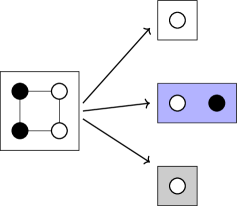
Each row of the map corresponds to a different type of stabilizer generator in the coarse-grained model. The entries in a row are the coefficients for expressing a new stabilizer generator as a linear combination of the original stabilizer generators within the coarse-grained unit cell,
| (155) |
Here, , and are the translation variables of the original lattice. For the choice of coarse-graining map described in Sec. II.2.5, the original stabilizer generators within the coarse-grained unit cell are ordered as follows
| (156) |
According to the above ordering, the position of each stabilizer generator in the coarse-grained unit cell can be mapped to unit vectors . This implies, for example, that the generator originally at position becomes the generator in the coarse-grained unit cell, corresponding to the unit vector , and similarly the generator at position becomes the last, corresponding to .
As mentioned above, for all examples studied we have found that a copy of the original model appears after one step of ER. To find the QSS by looking for fixed point excitations under quotient ERG flow using the map, we need to consider only those rows that correspond to the copy of the original model on the coarse-grained lattice. For a CSS model with one type of stabilizer generator, we need to consider only one row of the map, denoted . This map, , specifies how type of excitations flow under quotient ER. The quotienting out of excitations that flow into self-bifurcating B models is achieved by ignoring the corresponding rows in , which specify how excitations flow to those B models. The fixed points of capture the potentially nontrivial QSS.
To find the fixed points of we take the infrared limit, corresponding to many steps of ER, after which an arbitrary excitation will be supported on the coarse-grained unit cell. This allows us to restrict our attention to columns that contain only entries with no polynomial variables. We then utilize the mapping from polynomials to unit vectors described below Eq. (156) to translate the monomials in into columns, resulting in a square matrix with entries, which we also denote . With this replacement, the flow of excitations within the unit cell of a quotient fixed point model under quotient ER has been specified. The fixed points of , after the replacement, provide representatives for the QSS. Several examples are worked out below.
V.0.1 X-cube model
Under ER, the X-cube model is mapped to itself, stacks of 2D toric code along each axis, and decoupled trivial qubits. In the Quotient Superselection Sectors section of the supplementary MATHEMATICA file SMERG.nb, column 8 contains the X-stabilizer term of X-cube model while Columns 11 and 19 contain the Z stabilizer terms. The map can be found in terms of the column operations used during ER, as described above. The row corresponding to the X-stabilizer term of X-cube in the map , i.e. , is given by
where , and are again translation variables on the coarse-grained lattice. Using the fact that the charge configuration given by is trivial in the X-cube model, we rewrite this row as
To capture the flow of excitations from the coarse-grained unit cell to the new copy of X-cube produced by ER, we write this row in terms of unit vectors as described above in Eq. (156). The entries are replaced by column vectors
where . Here, specifies that all stabilizer excitations within the unit cell flow to the stabilizer excitation at position of the new copy of X-cube on the coarse-grained lattice under quotient ER. Accordingly, the fixed point of this matrix is simply , corresponding to the fracton excitation from the -sector of the X-cube model.
On the other hand, the -sector splits into 16 different stabilizer terms during ER. Hence there are 16 columns in the map . The rows corresponding to the two -stabilizer terms in the copy of X-cube on the coarse-grained lattice are
Using the triviality of charge configurations and in the X-cube model, we rewrite these rows as
Again, converting the position labels to unit vectors, we obtain the map for the flow of excitations
where . The fixed points are
| and |
which correspond to the two generating lineons in the Z-sector of the X-cube model. Hence we find that the QSS group of X-cube is given by , which agrees with the result in Ref. Shirley et al., 2018c.
V.0.2 Cubic code 1
After ER, cubic code 1 bifurcates into a copy of itself, cubic code B and some disentangled trivial qubits. The matrix is given by
Using the triviality of the charge configuration in cubic code 1, we rewrite this row as
which specifies the flow of excitations into the CC1 model on the coarse-grained lattice. Converting the position labels into unit vectors, we can write this as a matrix
| (157) |
This means, for example, that the -excitation at position in the unit cell shown flows to an excitation of the -stabilizer at position in the coarse-grained lattice. Considering the next-coarse-grained unit cell, this position is equivalently expressed by the unit vector . The fixed point of the matrix in Eq. (157) is which corresponds to the fracton in -sector of cubic code 1. We remark that the -sector behaves similarly due to the relation between sectors in the cubic codes and hence the QSS group is given by .
In Fig. 14, we depict how the excited stabilizer at position splits into different excitations in the new models after ER. One of the split excitations is supported in the copy of the original model CC1 and hence the excitation at position on the original lattice flows to the nontrivial fixed point under quotient ER and therefore is in the nontrivial QSS. In addition, both stabilizers of are excited and the local stabilizer on a decoupled qubit is excited. The excitation in the coarse-grained lattice of CC1 is found at position in the next-coarse-grained unit cell. Upon further quotient ER, the excitation remains at position as it is a fixed point.
V.0.3 Cubic code 11
Cubic code 11 supports fractons, lineons and planons, where the lineons and planons are composites of fractons. Under ER, cubic code 11 splits into itself, a self-bifurcating lineon model and a stack of 2D toric codes. In this case, the map is given by
Using the triviality of charge configurations and in cubic code 11, we rewrite as
Converting the position labels to unit vectors, we get find the matrix
whose only nonzero fixed point is given by . Since the -sector behaves similarly we find that the QSS group is .
VI Discussions and Conclusions
In this work we have systematically studied unconventional bifurcating ERG flows of gapped stabilizer Hamiltonian models. We introduced the notions of self-bifurcating and quotient bifurcating fixed points to organize the possible behavior of bifurcating fixed point models. This inspired us to define the notion of bifurcated equivalence class, generalizing the conventional notion of gapped phase and foliated fracton equivalence. This also led to a natural definition of quotient superselection sectors. These ideas were then brought to bear on a large range of stabilizer model examples, including 17 of Haah’s cubic codes and Yoshida’s fractal spin liquids. All models were found to be bifurcating ERG fixed points. Furthermore, many cubic codes and all first-order fractal spin liquids were found to be self-bifurcating. These results are summarized in table 1.
We found that the long-range entanglement features of stabilizer models provide insights into their structure. The mobilities of particles in each model was found to constrain the nature of the self-bifurcating models produced by ER. For models that support planon particles, we found that a stack of 2D toric codes could be extracted during ER. For example, CC11 supports planons with mobility in the lattice planes perpendicular to and consequently a stack of 2D toric codes is extracted during ER. This leads us to conjecture Dua (2019) that the existence of a planon in a 3D translation-invariant topological stabilizer model implies that a copy of the 2D toric code can be extracted via a local unitary transformation. Extending this in a translation-invariant way leads to the observed extraction of a stack of 2D toric codes. We also conjecture that if the original model has a particle with three dimensional mobility, a 3D toric code can be extracted via a local unitary circuit.
Models in which all the elementary excitations can move along a certain direction are observed to be invariant under ER that coarse-grains along . This is consistent with the fact that the number of encoded qubits does not change as the system size grows along this particular direction i.e. . Conversely, it was shown in Ref. Yoshida, 2011 that all particles must have three-dimensional mobility in any 3D topological stabilizer model that has a constant ground space degeneracy as the system size increases along all three axes, and hence such models are in TQFT-type phases. Inspired by this result, we conjecture that this principle can be extended to cover models with a ground space degeneracy that is constant as the system size grows along two axes, in which case we posit that all particles in the theory must be at least mobile in a 2D plane spanned by the two axes, and consequently the model must be a stack of planon and TQFT models. Similarly we conjecture for models with a ground space degeneracy that is constant as the system size grows along one axis, that all particles must be at least mobile along that axis, and consequently such a model is a stack of lineon, planon and TQFT models. Combining this with conjectures posed previously in Ref. Dua et al., 2019a: that all TQFT stabilizer models are equivalent to copies of the 3D toric code (possibly with fermionic point particle) and planon stabilizer models are equivalent to a stack of 2D toric codes, and the fact that lineon models can be compactified Dua et al. (2019b) along the lineon direction to produce 2D subsystem symmetry breaking models, points the way towards general classification results for 3D translation-invariant topological stabilizer models, inspired by the ERG flows we have found in examples. We leave the proofs of these conjectures to a future work.
For bifurcating models, when there is an additive correction to the exponential scaling of the number of encoded qubits as the system size increases by a factor , i.e. , the model cannot self-bifurcate under coarse graining by . For models that do self-bifurcate, the additive correction vanishes i.e. . We have calculated the number of encoded qubits for many examples over a range of system sizes, see table 4 in the appendix, and confirmed that they are consistent with the ERG flows found in table 1. We remark that a correction to the linear scaling of was the first indication that X-cube is a nontrivial foliated model Vijay et al. (2016). It would be interesting to search for invariant quantities that characterize nontrivial bifurcated models, such as the correction or similarly inspired corrections to entanglement entropy, generalizing ideas that arose in the study of foliated fracton models Shirley et al. (2019b).
Our examples have focused on coarse-graining by a factor of two, which appeared natural for qubit systems. In particular each quotient fixed point example is bifurcated equivalent to itself on all lattices with spacings that are related by a multiple of two. It would be interesting to extend this to other primes, in an attempt to remove the lattice scale entirely from the bifurcated equivalence class of these models.
We also note the appearance of the 2-adic norm of (for lattice spacing ) in the ratio of the number of quotient fixed point branches to all branches, the vast majority of which are generated by self-bifurcating B models, when one starts with an initial system on the 3D torus and applies ERG until all factors of have been removed from . Similarly for the ratio should be given by the 2-adic norm of . The further appearance of -adic norms in fracton models remains an intriguing prospect.
The bifurcating ER concepts and methods employed here apply equally well to subsystem symmetry breaking models. It would be interesting if they could shed light onto the classification of 2D translation-invariant spontaneous symmetry breaking stabilizer models, which has been accomplished in 1D Haah (2013b) but remains open in 2D due to the presence of complicated fractal like symmetries Williamson (2016); Yoshida (2013). This classification problem appears to be contained within the classification of 3D translation-invariant topological stabilizer models due to the existence of lineon models that can be compactified along the lineon direction to produce any known 2D subsystem symmetry breaking model. The bifurcating ER methods can also be extend directly to subsystem symmetry-protected topological phases (SSPT), by imposing a subsystem symmetry constraint on the individual gates in each ER step. This should shed light on the question: what is the appropriate definition of SSPT equivalence class? Devakul et al. (2018c); Devakul (2018b); Shirley et al. (2019d)
It would also be interesting to extend the ERG approach applied in this work to fractonic U(1) tensor gauge theories Pretko (2017a, b). It has been found that upon Higgsing such theories may transition to either fractonic or conventional topological orders Ma et al. (2018); Bulmash and Barkeshli (2018a, b); Williamson et al. (2018), so it raises the question of how the “parent” fractonic U(1) gauge theories behave under ERG.
Finally, exact ERG flows have been found for TQFT Hamiltonians beyond stabilizer models König et al. (2009). It would be interesting to extend these ERG flows to bifurcating ERG flows for nonabelian fracton models Prem et al. (2019); Song et al. (2019b). It is currently unclear if foliated equivalence extends straightforwardly to nonabelian fracton models as their ground state degeneracies behave somewhat differently to the abelian case Song et al. (2019a).
Note added: During the writing of this paper we learnt of the work by Shirley, Slagle and Chen on closely related topics Shirley et al. (2019c).
Acknowledgements.
AD and DW thank Jeongwan Haah for useful discussions. DW also thanks Yichen Hu and Abhinav Prem. PS thanks Jayameenakshi Venkatraman for introducing him to quantum error correction. This work is supported by start-up funds at Yale University (DW and MC), NSF under award number DMR-1846109 and the Alfred P. Sloan foundation (MC).References
- Wilson (1975) K. G. Wilson, The renormalization group: Critical phenomena and the Kondo problem, Rev. Mod. Phys. 47, 773 (1975).
- Haah (2014) J. Haah, Bifurcation in entanglement renormalization group flow of a gapped spin model, Phys. Rev. B 89, 75119, arXiv:1310.4507 (2014).
- Vidal (2007) G. Vidal, Entanglement renormalization, Phys. Rev. Lett. 99, 220405, arXiv:cond-mat/0512165 (2007).
- König et al. (2009) R. König, B. W. Reichardt, and G. Vidal, Exact entanglement renormalization for string-net models, Phys. Rev. B 79, 10.1103/PhysRevB.79.195123, arXiv:0806.4583 (2009).
- Aguado and Vidal (2008) M. Aguado and G. Vidal, Entanglement renormalization and topological order, Phys. Rev. Lett. 100, 070404, arXiv:0712.0348 (2008).
- Haah (2018) J. Haah, Classification of translation invariant topological Pauli stabilizer codes for prime dimensional qudits on two-dimensional lattices, arXiv:1812.11193 (2018).
- Bombin et al. (2012) H. Bombin, G. Duclos-Cianci, and D. Poulin, Universal topological phase of two-dimensional stabilizer codes, New J. Phys. 14, 73048, arXiv:1103.4606 (2012).
- Bombín (2014) H. Bombín, Structure of 2D Topological Stabilizer Codes, Commun. Math. Phys. 327, 387, arXiv:1107.2707 (2014).
- Chamon (2005) C. Chamon, Quantum glassiness in strongly correlated clean systems: An example of topological overprotection, Phys. Rev. Lett. 94, 40402, arXiv:cond-mat/0404182 (2005).
- Castelnovo et al. (2010) C. Castelnovo, C. Chamon, and D. Sherrington, Quantum mechanical and information theoretic view on classical glass transitions, Phys. Rev. B 81, 184303, arXiv:1003.3832 (2010).
- Bravyi et al. (2010) S. Bravyi, B. Leemhuis, and B. M. Terhal, Topological order in an exactly solvable 3D spin model, Ann. Phys. 326, 839, arXiv:1006.4871 (2010).
- Castelnovo and Chamon (2012) C. Castelnovo and C. Chamon, Topological quantum glassiness, Philosophical Magazine 92, 304, arXiv:1108.2051 (2012).
- Ma et al. (2017) H. Ma, E. Lake, X. Chen, and M. Hermele, Fracton topological order via coupled layers, Phys. Rev. B 95, 245126, arXiv:1701.00747 (2017).
- Vijay et al. (2016) S. Vijay, J. Haah, and L. Fu, Fracton Topological Order, Generalized Lattice Gauge Theory and Duality, Phys. Rev. B 94, 235157, arXiv:1603.04442 (2016).
- Williamson (2016) D. J. Williamson, Fractal symmetries: Ungauging the cubic code, Phys. Rev. B 94, 155128, arXiv:1603.05182 (2016).
- Vijay (2017) S. Vijay, Isotropic Layer Construction and Phase Diagram for Fracton Topological Phases, arXiv:1701.00762 (2017).
- Vijay and Fu (2017) S. Vijay and L. Fu, A Generalization of Non-Abelian Anyons in Three Dimensions, arXiv:1706.07070 (2017).
- Slagle and Kim (2017) K. Slagle and Y. B. Kim, Fracton topological order from nearest-neighbor two-spin interactions and dualities, Phys. Rev. B 96, 165106, arXiv:1704.03870 (2017).
- Halász et al. (2017) G. B. Halász, T. H. Hsieh, and L. Balents, Fracton Topological Phases from Strongly Coupled Spin Chains, Phys. Rev. Lett. 119, 257202, arXiv:1707.02308 (2017).
- Devakul (2018a) T. Devakul, topological order in the face-centered-cubic quantum plaquette model, Phys. Rev. B 97, 155111, arXiv:1712.05377 (2018a).
- Devakul et al. (2018a) T. Devakul, S. A. Parameswaran, and S. L. Sondhi, Correlation function diagnostics for type-I fracton phases, Phys. Rev. B 97, 41110, arXiv:1709.10071 (2018a).
- Prem et al. (2019) A. Prem, S.-J. Huang, H. Song, and M. Hermele, Cage-net fracton models, Phys. Rev. X 9, 021010, arXiv:1806.04687 (2019).
- Bulmash and Iadecola (2019) D. Bulmash and T. Iadecola, Braiding and gapped boundaries in fracton topological phases, Phys. Rev. B 99, 125132, arXiv:1810.00012 (2019).
- Song et al. (2019a) H. Song, A. Prem, S.-J. Huang, and M. A. Martin-Delgado, Twisted fracton models in three dimensions, Phys. Rev. B 99, 155118, arXiv:1805.06899 (2019a).
- Brown and Williamson (2019) B. J. Brown and D. J. Williamson, Parallelized quantum error correction with fracton topological codes, arXiv:1901.08061 (2019).
- Weinstein et al. (2018) Z. Weinstein, E. Cobanera, G. Ortiz, and Z. Nussinov, Absence of finite temperature phase transitions in the x-cube model and its zp generalization, arXiv:1812.04561 (2018).
- Hsieh and Halász (2017) T. H. Hsieh and G. B. Halász, Fractons from partons, Phys. Rev. B 96, 165105, arXiv:1703.02973 (2017).
- Prem and Williamson (2019) A. Prem and D. J. Williamson, Gauging permutation symmetries as a route to non-Abelian fractons, arXiv:1905.06309 (2019).
- Bulmash and Barkeshli (2019) D. Bulmash and M. Barkeshli, Gauging fractons: immobile non-Abelian quasiparticles, fractals, and position-dependent degeneracies, arXiv:1905.05771 (2019).
- Dua et al. (2019a) A. Dua, I. H. Kim, M. Cheng, and D. J. Williamson, Sorting topological stabilizer models in three dimensions, arXiv:1908.08049 (2019a).
- Dua et al. (2019b) A. Dua, D. J. Williamson, J. Haah, and M. Cheng, Compactifying fracton stabilizer models, Phys. Rev. B 99, 245135, arXiv:1903.12246 (2019b).
- Evenbly and Vidal (2014a) G. Evenbly and G. Vidal, Real-Space Decoupling Transformation for Quantum Many-Body Systems, Phys. Rev. Lett. 112, 220502 (2014a).
- Evenbly and Vidal (2014b) G. Evenbly and G. Vidal, Class of Highly Entangled Many-Body States that can be Efficiently Simulated, Phys. Rev. Lett. 112, 240502 (2014b).
- Evenbly and Vidal (2014c) G. Evenbly and G. Vidal, Scaling of entanglement entropy in the (branching) multiscale entanglement renormalization ansatz, Phys. Rev. B 89, 235113 (2014c).
- Chen et al. (2010) X. Chen, Z. C. Gu, and X. G. Wen, Local unitary transformation, long-range quantum entanglement, wave function renormalization, and topological order, Phys. Rev. B 82, 155138, arXiv:1004.3835 (2010).
- Swingle and McGreevy (2016a) B. Swingle and J. McGreevy, Renormalization group constructions of topological quantum liquids and beyond, Phys. Rev. B 93, 045127 (2016a).
- Swingle and McGreevy (2016b) B. Swingle and J. McGreevy, Mixed -sourcery: Building many-body states using bubbles of nothing, Phys. Rev. B 94, 155125 (2016b).
- Shirley et al. (2019a) W. Shirley, K. Slagle, and X. Chen, Foliated fracton order from gauging subsystem symmetries, SciPost Phys. 6, 41, arXiv:1806.08679 (2019a).
- Shirley et al. (2018a) W. Shirley, K. Slagle, Z. Wang, and X. Chen, Fracton models on general three-dimensional manifolds, Phys. Rev. X 8, 031051, arXiv:1712.05892 (2018a).
- Shirley et al. (2018b) W. Shirley, K. Slagle, and X. Chen, Foliated fracton order in the checkerboard model, arXiv:1806.08633 (2018b).
- Shirley et al. (2019b) W. Shirley, K. Slagle, and X. Chen, Universal entanglement signatures of foliated fracton phases, SciPost Phys. 6, 1, arXiv:1803.10426 (2019b).
- Shirley et al. (2018c) W. Shirley, K. Slagle, and X. Chen, Fractional excitations in foliated fracton phases, arXiv:1806.08625 (2018c).
- Haah (2011) J. Haah, Local stabilizer codes in three dimensions without string logical operators, Phys. Rev. A 83, 42330, arXiv:1101.1962 (2011).
- Yoshida (2013) B. Yoshida, Exotic topological order in fractal spin liquids, Phys. Rev. B 88, 125122, arXiv:1302.6248 (2013).
- Zeng et al. (2019) B. Zeng, X. Chen, D.-L. Zhou, and X.-G. Wen, Quantum Information Meets Quantum Matter, economy ed., Quantum Science and Technology (Springer-Verlag New York, 2019) pp. XXII, 364.
- Hastings and Wen (2005) M. B. Hastings and X. G. Wen, Quasiadiabatic continuation of quantum states: The stability of topological ground-state degeneracy and emergent gauge invariance, Phys. Rev. B 72, 45141, arXiv:cond-mat/0503554 (2005).
- Haah et al. (2018) J. Haah, L. Fidkowski, and M. B. Hastings, Nontrivial Quantum Cellular Automata in Higher Dimensions, arXiv:1812.01625 (2018).
- Kitaev (2003) A. Y. Kitaev, Fault-tolerant quantum computation by anyons, Ann. Phys. 303, 2, arXiv:quant-ph/9707021 (2003).
- Levin and Wen (2005) M. A. Levin and X. G. Wen, String-net condensation: A physical mechanism for topological phases, Phys. Rev. B 71, 045110, arXiv:cond-mat/0404617 (2005).
- Koenig et al. (2010) R. Koenig, G. Kuperberg, and B. W. Reichardt, Quantum computation with Turaev-Viro codes, Ann. Phys. 325, 2707, arXiv:1002.2816 (2010).
- Walker and Wang (2012) K. Walker and Z. Wang, (3+1)-TQFTs and topological insulators, Frontiers of Physics 7, 150, arXiv:1104.2632 (2012).
- Williamson and Wang (2017) D. J. Williamson and Z. Wang, Hamiltonian models for topological phases of matter in three spatial dimensions, Ann. Phys. 377, 311, arXiv:1606.07144 (2017).
- Calderbank and Shor (1996) A. R. Calderbank and P. W. Shor, Good quantum error-correcting codes exist, Phys. Rev. A 54, 1098, arXiv:quant-ph/9512032 (1996).
- Steane (1996) A. Steane, Multiple-particle interference and quantum error correction, Proc. Roy. Soc. Lond. A 452, 2551, arXiv:quant-ph/9601029 (1996).
- Imai (1977) H. Imai, A theory of two-dimensional cyclic codes, Information and Control 34, 1 (1977).
- MacWilliams and Sloane (1977) F. J. MacWilliams and N. J. A. Sloane, The theory of error-correcting codes (North-Holland Publishing Co., Amsterdam-New York-Oxford, 1977) pp. i–ix and 1–762, north-Holland Mathematical Library, Vol. 16.
- Güneri and Özbudak (2008) C. Güneri and F. Özbudak, Multidimensional cyclic codes and artin–schreier type hypersurfaces over finite fields, Finite Fields and Their Applications 14, 44 (2008).
- Haah (2013a) J. Haah, Commuting Pauli Hamiltonians as Maps between Free Modules, Commun. Math. Phys. 324, 351, arXiv:1204.1063 (2013a).
- Haah (2013b) J. Haah, Lattice quantum codes and exotic topological phases of matter, arXiv:1305.6973 (2013b).
- Devakul et al. (2018b) T. Devakul, Y. You, F. J. Burnell, and S. L. Sondhi, Fractal Symmetric Phases of Matter, arXiv:1805.04097 (2018b).
- Devakul and Williamson (2018) T. Devakul and D. J. Williamson, Universal quantum computation using fractal symmetry-protected cluster phases, Phys. Rev. A 98, 022332, arXiv:1806.04663 (2018).
- Stephen et al. (2018) D. T. Stephen, H. P. Nautrup, J. Bermejo-Vega, J. Eisert, and R. Raussendorf, Subsystem symmetries, quantum cellular automata, and computational phases of quantum matter, arXiv:1806.08780 (2018).
- Devakul (2018b) T. Devakul, Classifying local fractal subsystem symmetry protected topological phases, arXiv:1812.02721 (2018b).
- Daniel et al. (2019) A. K. Daniel, R. N. Alexander, and A. Miyake, Computational universality of symmetry-protected topologically ordered cluster phases on 2D Archimedean lattices, arXiv:1907.13279 (2019).
- Shirley et al. (2019c) W. Shirley, K. Slagle, and X. Chen, Entanglement Renormalization of Fractonic Gauge Theories (in preparation), (2019c).
- Haah (2016) J. Haah, Algebraic Methods for Quantum Codes on Lattices, Revista Colombiana de Matemáticas 50, 299, arXiv:1607.01387 (2016).
- Yoshida (2011) B. Yoshida, Classification of quantum phases and topology of logical operators in an exactly solved model of quantum codes, Ann. Phys. 326, 15, arXiv:1007.4601 (2011).
- Levin and Wen (2003) M. Levin and X.-G. Wen, Fermions, strings, and gauge fields in lattice spin models, Phys. Rev. B 67, 245316 (2003).
- Slagle et al. (2019) K. Slagle, D. Aasen, and D. Williamson, Foliated field theory and string-membrane-net condensation picture of fracton order, SciPost Phys. 6, arXiv:1812.01613 (2019).
- Wang et al. (2019) T. Wang, W. Shirley, and X. Chen, Foliated fracton order in the Majorana checkerboard model, arXiv:1904.01111 (2019).
- Dua (2019) A. Dua, Unpublished (2019).
- Devakul et al. (2018c) T. Devakul, D. J. Williamson, and Y. You, Classification of subsystem symmetry-protected topological phases, Phys. Rev. B 98, 235121, arXiv:1808.05300 (2018c).
- Shirley et al. (2019d) W. Shirley, K. Slagle, and X. Chen, Twisted foliated fracton phases, arXiv:1907.09048 (2019d).
- Pretko (2017a) M. Pretko, Subdimensional particle structure of higher rank U(1) spin liquids, Phys. Rev. B 95, 115139, arXiv:1604.05329 (2017a).
- Pretko (2017b) M. Pretko, Generalized electromagnetism of subdimensional particles: A spin liquid story, Phys. Rev. B 96, 35119, arXiv:1606.08857 (2017b).
- Ma et al. (2018) H. Ma, M. Hermele, and X. Chen, Fracton topological order from the Higgs and partial-confinement mechanisms of rank-two gauge theory, Phys. Rev. B 98, 035111, arXiv:1802.10108 (2018).
- Bulmash and Barkeshli (2018a) D. Bulmash and M. Barkeshli, Higgs mechanism in higher-rank symmetric U(1) gauge theories, Phys. Rev. B 97, 235112, arXiv:1802.10099 (2018a).
- Bulmash and Barkeshli (2018b) D. Bulmash and M. Barkeshli, Generalized U(1) Gauge Field Theories and Fractal Dynamics, arXiv:1806.01855 (2018b).
- Williamson et al. (2018) D. J. Williamson, Z. Bi, and M. Cheng, Fractonic Matter in Symmetry-Enriched U(1) Gauge Theory, arXiv:1809.10275 (2018).
- Song et al. (2019b) H. Song, A. Prem, S.-J. Huang, and M. A. Martin-Delgado, Twisted fracton models in three dimensions, Phys. Rev. B 99, 155118 (2019b).
- Atiyah and Macdonald (2016) M. F. Atiyah and I. G. Macdonald, Introduction to commutative algebra, economy ed., Addison-Wesley Series in Mathematics (Westview Press, Boulder, CO, 2016) pp. ix+128.
- Adams and Loustaunau (1994) W. W. Adams and P. Loustaunau, An introduction to Gröbner bases, Graduate Studies in Mathematics, Vol. 3 (American Mathematical Society, Providence, RI, 1994).
Appendix A List of codes and their polynomial representations
In Table 3, we list the polynomials and for various cubic codes, denoted CCi where runs from 1 to 17, and their B-models if any, denoted CCBi. The stabilizer map for a cubic code in terms of and is given by
| (162) |
and the stabilizer ideal is defined as the ideal , which contains the polynomials in the image of the excitation map, see Eq. (82). The third column of the table below contains polynomial entries, each of which specifies the positions of two non-trivial clusters of charges that are created at the ends of string operators. For example, implies that the small segment of string operator in CC5 creates elementary excitations at and . This means that the direction of each string operator can be read off the binomial factor in its description.
| Model | Positions of charges in a trivial pair | ||
|---|---|---|---|
| CC1 | |||
| CC2 | |||
| CC3 | |||
| CC4 | |||
| CC5 | |||
| CC6 | |||
| CC7 | |||
| CC8 | |||
| CC9 | |||
| CC10 | |||
| CC11 | |||
| CC12 | |||
| CC13 | |||
| CC14 | |||
| CC15 | |||
| CC16gggCC16 is equivalent to CC15 after modular transformations. Hence, we don’t include explicitly here. | |||
| CC17 | |||
Appendix B Demonstrating our heuristic procedure for entanglement renormalization on the X-cube model
In this appendix, we outline our heuristic procedure for entanglement renormalization on CSS codes and demonstrate it, using the X-cube model as an example. The heuristic is quite simple, essentially we coarse grain until a monomial appears in a column. We next use that entry to set the rest of the column to 0 via CNOT gates. The monomial entry can then be used to set its row to 0 via column operations. After this the qubit has been disentangled into the trivial state and its row and column can be removed. This is repeated until there are no monomials left. At which point the model has either bifurcated or we perform more steps of coarse graining. There is an important subtlety to the above recipe, as we do not necessarily need a monomial to set the rest of a column and row to 0. In some cases, such as the X-cube example below, a non-monomial entry, pair of entries, or several entries, in a column can be used to set the rest of the column to zero. This more general step can be used in place of the monomial step mentioned above.
The stabilizer map for the X-cube model is given by
| (163) |
After coarse-graining in , the and sectors of the stabilizer map are respectively given by
| (164) |
where is now the translation variable in the coarse-grained unit cell. The goal is to decouple different models or stabilizer terms such that they are supported on non-overlapping sets of qubits. We first do this for the -sector. In doing so, the -sector will also get modified. In the two columns for the -sector, the and row elements in both columns are the same. Thus, applying the column operation Col simplifies the sectors of the stabilizer map
| (165) |
Now, since there are same polynomials in certain row elements of the first column, one can get rid of them by applying CNOT and CNOT such that the second column is not affected due to the zero entries in it.
| (166) |
Finally, applying CNOT and CNOT decouples the two stabilizer terms in the -sector as follows,
| (167) |
It turns out that once the -sector is decoupled, doing certain column operations in the -sector is enough to decouple the whole stabilizer map into two different models. This is also observed for other models. Applying Col, Col and Col gives
| (168) |
Removing the disentangled qubit (the 1st qubit), we have found that the model splits into two, one is given by
| (169) |
which is just a stack of 2D toric codes parallel to the plane, and the other is a coarse-grained X-cube model.
Appendix C Cubic codes as fractal spin liquids
Certain cubic codes could be mapped to the following fractal spin liquid (FSL) Yoshida (2013) form of the stabilizer map,
| (174) |
which represents a first-order FSL for and a second-order FSL otherwise. Here where denotes , or . In table 3, we write down the polynomials that appear in the FSL forms of various cubic codes. The explicit mapping from the cubic codes to FSLs is contained in the supplementary MATHEMATICA file SMERG.nb.
| Model | |||
|---|---|---|---|
| CC1 | |||
| CC2 | |||
| CC3 | |||
| CC5 | |||
| CC6 | 0 | ||
| CC9hhhCC9 is equivalent to CC5 |
Appendix D Numerical results on number of encoded qubits
In table 4, we list the number of encoded qubits w.r.t. system size in the cubic codes and the Sierpinski fractal spin liquid (SFSL) on an lattice. The results are calculated in the supplementary MATHEMATICA file encodedqubits.nb. Results for some of these models were recovered analytically in the next section using the polynomial framework.
| CC1 | CC2 | CC3 | CC4 | CC5 | CC6 | CC7 | CC8 | CC9 | CC10 | CC11 | CC12 | CC13 | CC14 | CC15 | CC16 | CC17 | SFSL | ||
|---|---|---|---|---|---|---|---|---|---|---|---|---|---|---|---|---|---|---|---|
| 2 | 6 | 4 | 4 | 4 | 4 | 4 | 4 | 4 | 4 | 4 | 4 | 4 | 8 | 4 | 4 | 4 | 8 | 0 | |
| 3 | 2 | 2 | 2 | 6 | 2 | 2 | 2 | 2 | 2 | 2 | 10 | 8 | 6 | 6 | 6 | 6 | 6 | 6 | 4 |
| 4 | 14 | 8 | 8 | 8 | 8 | 8 | 8 | 8 | 8 | 8 | 8 | 0 | 8 | 16 | 8 | 8 | 8 | 16 | 0 |
| 5 | 2 | 2 | 2 | 2 | 2 | 2 | 2 | 2 | 2 | 2 | 10 | 0 | 10 | 10 | 10 | 10 | 10 | 10 | 0 |
| 6 | 6 | 4 | 4 | 12 | 4 | 4 | 4 | 4 | 4 | 4 | 24 | 16 | 16 | 16 | 12 | 16 | 16 | 24 | 8 |
| 7 | 2 | 14 | 2 | 2 | 14 | 14 | 2 | 2 | 14 | 2 | 14 | 0 | 26 | 26 | 26 | 26 | 26 | 14 | 12 |
| 8 | 30 | 16 | 16 | 16 | 16 | 16 | 16 | 16 | 16 | 16 | 16 | 0 | 16 | 32 | 16 | 16 | 16 | 32 | 0 |
| 9 | 2 | 2 | 2 | 6 | 2 | 2 | 2 | 2 | 2 | 2 | 22 | 8 | 18 | 18 | 18 | 18 | 18 | 18 | 4 |
| 10 | 6 | 4 | 4 | 4 | 4 | 4 | 4 | 4 | 4 | 4 | 20 | 0 | 20 | 24 | 20 | 20 | 20 | 40 | 0 |
| 11 | 2 | 2 | 2 | 2 | 2 | 2 | 2 | 2 | 2 | 2 | 22 | 0 | 22 | 22 | 22 | 22 | 22 | 22 | 0 |
| 12 | 14 | 8 | 8 | 24 | 8 | 8 | 8 | 8 | 8 | 8 | 52 | 32 | 36 | 32 | 24 | 36 | 36 | 56 | 16 |
| 13 | 2 | 2 | 2 | 2 | 2 | 2 | 2 | 2 | 2 | 2 | 26 | 0 | 26 | 26 | 26 | 26 | 26 | 26 | 0 |
| 14 | 6 | 28 | 4 | 4 | 28 | 28 | 4 | 4 | 28 | 4 | 28 | 0 | 52 | 56 | 52 | 52 | 52 | 56 | 24 |
| 15 | 50 | 2 | 18 | 22 | 26 | 26 | 42 | 42 | 26 | 18 | 82 | 56 | 54 | 54 | 54 | 54 | 54 | 78 | 28 |
| 16 | 62 | 32 | 32 | 32 | 32 | 32 | 32 | 32 | 32 | 32 | 32 | 0 | 32 | 64 | 32 | 32 | 32 | 64 | 0 |
| 17 | 2 | 2 | 2 | 2 | 2 | 2 | 2 | 2 | 2 | 2 | 34 | 0 | 34 | 34 | 34 | 34 | 34 | 34 | 0 |
| 18 | 6 | 4 | 4 | 12 | 4 | 4 | 4 | 4 | 4 | 4 | 48 | 16 | 40 | 40 | 36 | 40 | 40 | 72 | 8 |
| 19 | 2 | 2 | 2 | 2 | 2 | 2 | 2 | 2 | 2 | 2 | 38 | 0 | 38 | 38 | 38 | 38 | 38 | 38 | 0 |
| 20 | 14 | 8 | 8 | 8 | 8 | 8 | 8 | 8 | 8 | 8 | 40 | 0 | 40 | 48 | 40 | 40 | 40 | 80 | 0 |
.
Appendix E Number of encoded qubits
In Ref. Haah, 2013a, Haah used techniques from commutative algebra to derive a formula for the number of encoded qubits for the cubic code CC1 which we recount in Subsection E.1. We use the general strategy used by Haah to derive similar formulas for the number of encoded qubits for other cubic codes. We consider CC6 and CC11 as examples. We first explain the general definitions and explain the steps used by Haah in his derivation.
Suppose is an ideal corresponding to a code. Fix some . Imposing the periodicity conditions , the number of encoded qubits is given by
where is the dimension of as a vector space and is the ideal defined as
Due to algebrogeometric reasons, it is preferable to work over an algebraically closed field. Hence we take the algebraic closure . By extension of scalars of the vector spaces, we have
where is now the ideal generated in . In order to calculate this, we use the structure theorem for Artinian rings from (Atiyah and Macdonald, 2016, Theorem 8.7) which we restate in Theorem 1.
Theorem 1.
Let be an Artinian ring. Then for some where is a local Artinian ring for all integers . Moreover, the decomposition is unique up to isomorphism.
Remark.
In the above theorem, if is also a vector space over , we have and in particular .
We apply Theorem 1 to obtain the formula where
and the sum is taken over all maximal ideals . By the weak form of Hilbert’s Nullstellensatz, any maximal ideal is of the form where , i.e., satisfies
In particular . Since , we also have and similarly, . We now calculate for all maximal ideals .
Fix a maximal ideal . Now write where and . Consider the factorization
The right most factor has no further factors of since putting results in since and . We obtain similar factorization for the variables and . We recognize that and similarly for the variables and since , which motivates us to define the ideal
where , and . We have the canonical map since . We would like to apply (Atiyah and Macdonald, 2016, Corollary 3.2) which we restate in Lemma 1.
Lemma 1.
Let and be rings and be a multiplicatively closed set. If is a ring homomorphism such that
-
1.
for all , the element is a unit
-
2.
for all , we have for some
-
3.
for all , there are and such that
then there is a unique isomorphism such that where is the canonical homomorphism.
Checking conditions of Lemma 1, we have the isomorphism
as rings and hence also as -modules which are of course simply vector spaces over . Thus we need to calculate . Note that if , then is the residue field at and hence we simply get . We assume henceforth.
Most of the time we can eliminate one of the three variables, say , and use the substitutions and to show , as rings and hence as vector spaces over , where , , and is the polynomial derived from and by eliminating the variable . This further simplifies the problem to the calculation of . In the following sections, we calculate this for various cubic codes by first finding appropriate Gröbner bases with the help of the computer algebra system SageMath. SageMath cannot calculate Gröbner bases for a general but we test various values of to accurately predict the Gröbner bases in terms of and then we prove that it is indeed so. Then we use the Gröbner bases to calculate . To calculate this, we use (Adams and Loustaunau, 1994, Proposition 2.1.6) which we restate in Theorem 2.
Theorem 2.
Let and be a polynomial ring endowed with a monomial ordering. Let be an ideal and be a Gröbner basis for . Then the set
is a basis for the vector space over .
Finally, we use , where the sum is over all maximal ideals , which is feasible to compute explicitly whenever we can explicitly count the number of points in certain appropriate subvarieties of .
Remark.
All Gröbner bases in the rest of the document are using the lexicographic ordering of monomials with . Polynomial divisions with respect to a Gröbner basis are also using the same ordering of monomials.
Remark.
We often need the roots of the polynomial which are the primitive cube roots of unity. We denote by any choice of a primitive th root of unity, for all .
E.1 Cubic code 1
The stabilizer generators of cubic code 1 (CC1) are given by
| (192) |
Hence, the stabilizer ideal that defines CC1 is . We eliminate the variable and use the substitutions and to obtain
Recalling definitions, we know that where such that . The last equation is satisfied if and only if or . In the latter case is a primitive cube root of unity and we assume the choice .
Lemma 2.
For the ideal , we have the following Gröbner bases.
-
1.
Suppose . Then
is a Gröbner basis.
-
2.
Suppose with . Then
is a Gröbner basis.
Proof.
It is a straight forward calculation using the S-polynomials of Buchberger’s algorithm to verify that is a Gröbner basis for the ideal for all the cases. It is also a straight forward calculation by polynomial divisions by elements in to verify that for all the cases. It remains to show that for all the cases. This is shown below assuming the same hypotheses and using the same set as in the lemma for the corresponding cases.
Case 1. The only nontrivial containment we need to show is , i.e., . This follows if we show our claim for all integers by taking the case because . We show this by induction. The base case is trivial. Suppose that the claim holds for some integer , i.e., . Squaring this and using , we get
where we use the fact that by Fermat’s little theorem or by directly checking both cases and .
Case 2. The only nontrivial containment we need to show is , i.e., . The equation holds for all integers in this case as well. The proof is exactly the same as above. By hypothesis, . Using the case and multiplying by , we get
∎
Now we simply read off the dimension using the Gröbner basis and obtain the formula
Recalling definitions, the above gives the formula
Now we wish to calculate where the sum is over all maximal ideals . For the calculation, we first need to explicitly calculate the points in the variety . To solve , we divide by to get and hence the solutions are . Thus we calculate that the solutions of is the set of points where
Note that the intersection is which consists of the only point satisfying . Imposing the periodic conditions , we have the corresponding set of solutions where for all . The intersection is . Thus, and
we put everything together using the formula
| (193) | ||||
| (194) |
In general, it is difficult to obtain a more explicit formula. However, we obtain a more explicit formula for some special cases.
First suppose . Then it is easy to see that is a greatest common divisor in Eq. 194. Hence Eq. 194 gives .
Now suppose for some . Then we have the factorization
We apply the same equation for and to get the factorization
Let be a root of the second factor . Suppose that . In this case we have
So implies which is a contradiction. Suppose that . In this case we have
So implies
Thus . But then
Thus, in any case, there is no common root among the second factors. So is a greatest common divisor in the Eq. 194. Now Eq. 194 gives .
Now suppose for some . We calculate that
Thus we have the factorization
We apply the same equation for and to get the factorizations
It is easy to see that is a greatest common divisor in Eq. 194 whose degree is . Using this in Eq. 194 gives .
Now suppose for some . Suppose is a root of . We calculate that
Thus we have the factorization
We apply the same equation for and to get the factorizations
Suppose is a root of the second factor . By multiplying by , we find that , i.e., is a th root of unity. Similarly, so are and . But then we have
which is a contradiction because for all . Thus is a greatest common divisor in Eq. 194. Now Eq. 194 gives . We summarize the results in the following theorem.
Theorem 3.
Consider CC1 defined by the ideal . Imposing the periodic conditions for some where and , the number of encoded qubits is given by
Moreover, we have the explicit formulas
Remark.
E.2 Cubic code 6
The stabilizer generators of cubic code 6 (CC6) are given by
| (212) |
Hence, the stabilizer ideal that defines CC6 is . We eliminate the variable to obtain
Recalling definitions, we know that where such that .
Lemma 3.
For the ideal , we have that
is a Gröbner basis.
Proof.
We assume the same hypotheses and use the same set as in the lemma. It is a straight forward calculation using the S-polynomials of Buchberger’s algorithm to verify that is a Gröbner basis for the ideal . It is also a straight forward calculation by polynomial divisions by elements in to verify that . It remains to show that .
The only nontrivial containment we need to show is , i.e., . We calculate that
Hence implies as desired. ∎
Now we simply read off the dimension using the Gröbner basis and obtain the formula
We wish to calculate where the sum is over all maximal ideals . For the calculation, we first need to explicitly calculate the points in the variety . By first finding solutions of , we easily calculate that the solutions of is the set of points . Imposing the periodic conditions , we have the corresponding set of solutions . Thus
Since , we can in fact simplify the equation to
We put everything together using the formula
In general, it is difficult to obtain a more explicit formula. We note however that calculating this for a single value of can already provide a formula for an infinite family of values of , namely, for all . It is not difficult to do this this explicitly by hand for small values of . We do this now for and .
First suppose . Then we have the factorizations
So we calculate that
Thus .
Now suppose . Then we have the factorizations
and
So because we check that and are not roots of by putting and . Again . Thus .
We summarize the results in the following theorem.
Theorem 4.
Consider CC6 defined by the ideal . Imposing the periodic conditions for some where and , the number of encoded qubits is given by
Moreover, we have the explicit formulas
Remark.
E.3 Cubic code 11
The stabilizer generators of cubic code 11 (CC11) are given by
| (230) |
Hence, the stabilizer ideal that defines CC11 is . We eliminate the variable and use the substitutions and to obtain
Recalling definitions, we know that where such that . The last equation is satisfied if and only if or .
Lemma 4.
For the ideal , we have the following Gröbner bases.
-
1.
Suppose and . Then we have the following cases.
-
(a)
Suppose . Then
is a Gröbner basis.
-
(b)
Suppose . Then
is a Gröbner basis.
-
(a)
-
2.
Suppose and . Then
is a Gröbner basis.
-
3.
Suppose and . Then
is a Gröbner basis.
Proof.
It is a straight forward calculation using the S-polynomials of Buchberger’s algorithm to verify that is a Gröbner basis for the ideal for all the cases. It is also a straight forward calculation by polynomial divisions by elements in to verify that for all the cases. It remains to show that for all the cases. This is shown below assuming the same hypotheses and using the same set as in the lemma for the corresponding cases.
Case 11.(a). The only nontrivial containment we need to show is , i.e., . We calculate that
The hypothesis implies with . Hence the hypothesis implies . Let . Realizing that , we multiply by to get
Case 11.(b). The only nontrivial containment we need to show is , i.e., . By a similar calculation as in the proof of Case 11.(a), we have
This time, the hypothesis implies . Hence
Let . Then the above implies . Again using , we multiply by to get
Case 2. The only nontrivial containment we need to show is , i.e., . This follows if we show our claim for all integers by taking the case. We show this by induction. The base case is trivial. Suppose that the claim holds for some integer , i.e., . Then
The hypothesis implies as desired.
Case 3. The only nontrivial containment we need to show is , i.e., . We have
Now by hypothesis. Let . Then the above implies . Thus
∎
Now we simply read off the dimensions using the Gröbner bases and obtain the formula
Recalling the definitions, the above gives the formula
Note that this holds if as well. Now we wish to calculate where the sum is over all maximal ideals . For the calculation, we first need to explicitly calculate the points in the variety . By first finding solutions of , we easily calculate that the solutions of is the set of points where
Note that the intersection is
which consists of the only points satisfying both and . Imposing the periodic conditions , we have the corresponding set of solutions where for all . The intersection is
Thus we immediately calculate
Note that and are in fact equal in all cases using any extension of specified by , noting that . We put everything together using the formula
| (231) | ||||
| (232) | ||||
In general, it is difficult to obtain a more explicit formula for the case . However, it is possible for a special case.
Suppose for some . We calculate that
Thus we have the factorization
We apply the same equation for and use to get the factorization
It is easy to see that is a greatest common divisor in Eq. 232 whose degree is . Using this in Eq. 232 gives .
We summarize the results in the following theorem.
Theorem 5.
Consider CC11 defined by the ideal . Imposing the periodic conditions for some where and , the number of encoded qubits is given by
Moreover, if for some , then we have the explicit formula
Remark.
E.4 Cubic code 11B
The stabilizer generators of cubic code 11B () are given by
| (250) |
Hence, the stabilizer ideal that defines is given by . We eliminate the variable to obtain
Recalling definitions, we know that , where such that . Notice that we have not made the substitutions in this example as the ideal is simple enough as it is.
Lemma 5.
For the ideal , we have the following Gröbner bases.
-
1.
Suppose . Then
is a Gröbner basis.
-
2.
Suppose . Then
is a Gröbner basis.
Proof.
It is a straight forward calculation using the S-polynomials of Buchberger’s algorithm to verify that is a Gröbner basis for the ideal for all the cases. It is also a straight forward calculation by polynomial divisions by elements in to verify that for all the cases. It remains to show that for all the cases. This is shown below assuming the same hypotheses and using the same set as in the lemma for the corresponding cases.
Case 1. The only nontrivial containment we need to show is , i.e., . We calculate that
The hypothesis implies with . Hence the hypothesis implies . Let . Realizing that , we multiply by to get
Now we simply read off the dimensions using the Gröbner bases and obtain the formula
Recalling the definitions, the above gives the formula
Now we wish to calculate where the sum is over all maximal ideals . For the calculation, we first need to explicitly calculate the points in the variety . By first finding solutions of , we easily calculate that the solutions of is the set of points where
Note that the intersection is . Imposing the periodic conditions , we have the corresponding set of solutions where for all . The intersection is . Thus, and
Recalling arguments from Subsection E.3, we put everything together using the formula
We also recall from Subsection E.3 that for the special case for some , we have the explicit calculation
We summarize the results in the following theorem.
Theorem 6.
Consider defined by the ideal . Imposing the periodic conditions for some where and , the number of encoded qubits is given by
Moreover, if for some , then we have the explicit formula
Remark.
Theorem 6 implies that as a function of , obeys the scaling relation
for all . This is consistent with the self-bifurcating behavior of .
Appendix F Charge annihilators
In our argument for choosing the coarse-graining factor to be 2, we argued how the charge annihilator or the set of trivial charges shows self-reproducing behavior under coarse-graining by a factor of 2. To be precise, the charge annihilator given by the stabilizer ideal changes to after coarse-graining. In the MATHEMATICA file SMERG.nb, we show the calculation for all the cubic codes. In fact, for all of them the annihilator after coarse-graining is given by where and are polynomials that give the stabilizer ideal as well as the charge annihilator of the original model. We now explain how we use elimination theory with Gröbner bases to compute the annihilator of the charge module after coarse-graining. The charge annihilator after coarse-graining is defined as the intersection of the original annihilator and the coarse-grained Laurent polynomial ring, i.e., .
Let and be a subring. Consider an ideal for some . We wish to compute the annihilator of the left -module . Since , we develop a method to compute .
Let and be a subring. Consider the ideal . Then elimination theory directly provides an algorithm to compute using a Gröbner basis according to (Adams and Loustaunau, 1994, Theorem 2.3.4). We now focus on arguing that computing is essentially the same as computing .
Define the surjective homomorphism uniquely determined by the mappings
Note that and . A simple set theoretic calculation gives . However, the reverse containment does not hold in general and this is the nontriviality which is to be shown.
Theorem 7.
We have . Hence, viewing as an ideal generated in , the charge annihilator after coarse-graining can be calculated by .
Proof.
First we show the useful fact . Define the surjective homomorphism uniquely determined by the mappings
and also define the surjective homomorphisms and in a similar fashion. Then we have the commutative diagram
In light of the containments
we have . Now, making the identification and using the division algorithm with the divisor being the monic polynomial , we conclude that . By similar arguments, we also have and . Thus .
We now compute that . Hence the surjective homomorphism lifts to the isomorphism . We use this and the second isomorphism theorem to get
More explicitly tracing the maps in the isomorphisms above, we have the commutative diagram
We see that the isomorphism is induced by the surjective homomorphism . This implies . Hence we conclude . ∎