Simulations of sawtooth-wave adiabatic passage with losses

Abstract

The results of simulations of cooling based on Sawtooth-Wave Adiabatic Passage (SWAP) are presented including the possibility of population leaking to states outside of the cycling transition. The amount of population leaking can be substantially suppressed compared to Doppler cooling, which could be useful for systems that are difficult to repump back to the cycling transition. The suppression of the leaked population was more effective when simulating the slowing of a beam than in cooling a thermal distribution. As expected, calculations of the leaked population versus branching ratio of spontaneous emission show that the suppression is more effective for narrow linewidth transitions. In this limit, using SWAP to slow a beam may be worth pursuing even when the branching ratio out of the cycling transition is greater than 10%.

I Introduction

The ability to laser cool atomsMetcalf and van der Straten (1999); Foot (2005) has enabled the exploration of collective behavior in atomic gases, ultracold scattering, and other effects. Methods used to laser cool atoms, as well as some variations, have been used for moleculesCarr et al. (2009) and nano- and micro-scale objectsNovotny and Hecht (2012). However, not all atoms, molecules, or nano-scale objects can be effectively laser cooled with known techniques, which motivates the search for new cooling methods.

Reference Norcia et al. (2018) described a method for laser cooling called Sawtooth-Wave Adiabatic Passage (SWAP) based on chirping counter-propagating light waves. This method was proposed for cooling narrow linewidth transitions. The basic idea is that Doppler shift of the counter-propagating light waves leads to a stimulated absorption from the beam opposite the atom’s velocity (due to the blue shift of that beam) followed by a stimulated emission from the beam propagating in the direction of the atom’s velocity (due to the red shift of that beam). If the linewidth is narrow, the spontaneous emission that occurs between the stimulated absorption and emission will be small. This leads to a momentum kick of $2\hbar k$, with $k$ the wavenumber of the light, opposite the velocity of the atom. Experimental results on the Sr ¹S₀ to ³P₁ transition with 7.5 kHz linewidth and calculations from a simple theoretical model supported both the possibility of cooling and the interpretation of the mechanism.

Reference Bartolotta et al. (2018) described in more detail the simple theoretical model for this process and presented the results from several simulations. Reference Petersen et al. (2019) performed SWAP cooling of Dy using a transition at 626 nm with a 136 kHz linewidth. This transition is $\sim 20\times$ broader than that in the demonstration on Sr. Reference Snigirev et al. (2019) described experimental results for SWAP cooling of Sr in a magneto-optical trap. These studiesNorcia et al. (2018); Bartolotta et al. (2018); Petersen et al. (2019); Snigirev et al. (2019); Liang et al. (2019) showed that SWAP gives a more rapid reduction of the kinetic energy compared to Doppler cooling, although the final temperature that can be reached is several times hotter than Doppler cooling. Finally, as first suggested in Ref. Norcia et al. (2018), SWAP cooling is promising for molecules because the loss of population to states outside of the cycling transition can be reduced due to the relative suppression of spontaneous emission. Reference Liang et al. (2019) calculated SWAP cooling for diatomic molecules in a magnetic field and did find a reduction in the population into leakage channels.

In this paper, we perform calculations for a more simplified case than Ref. Liang et al. (2019) to understand the role of leakage during SWAP cooling. For the model below, there is only one leak state and it can not be connected to the excited state by a laser transition. While not quite as realistic as Ref. Liang et al. (2019), this model allows for a more transparent interpretation of the results of the cooling when population can leak from the cycling transition. In particular, we present results on the performance of SWAP cooling as a function of branching ratio, ${\cal B}$, into the leak state for various spontaneous decay rates.

SWAP cooling for small ${\cal B}$ is important for molecules, but larger branching ratios might also be interesting. Part of our motivation was to determine whether SWAP is worth pursuing when this branching ratio is greater than 1/2. For example, laser cooling of antihydrogen, $\bar{\rm H}$, on the 1S-2P transition was predictedDonnan et al. (2013) to give an average final energy $\bar{E}_{f}\simeq 30$ mK compared to a Doppler temperature of $\sim 2$ mK. Because of the long lifetime of the 2S state, one could attempt SWAP cooling on the 2S-3P or 2S-4P transition to obtain colder $\bar{\rm H}$ which would improve, for example, the measurement of the 1S-2S transitionAhmadi and et al (ALPHA collaboration). Unfortunately, simulations below suggest that the short lifetime of these states and the unfavorable branching ratio preclude cooling $\bar{\rm H}$ by SWAP.

The results presented below suggest that SWAP with leaks to other states is more effective for slowing a beam of particles than for cooling. As expected, the quality of the SWAP cooling increases as the spontaneous decay rate decreases. However, for very narrow lines, SWAP might be useful even for branching ratios, ${\cal B}>0.1$.

II Theoretical model

All of the calculations used the model introduced in Ref. Bartolotta et al. (2018) with a couple modifications which will be explicitly noted.

The system is an atom with center of mass motion constrained to one dimension and with 3 internal states instead of the 2 internal states of Ref. Bartolotta et al. (2018). The translational motion is represented by momentum eigenstates which are stepped in units of the photon momentum, $\hbar k$ with $k$ the photon wavenumber. The two internal states treated in Ref. Bartolotta et al. (2018) are a ground state $|g\rangle$ and an excited state $|e\rangle$. To incorporate the possibility of population leaking to other states, the calculations below include a third state $|l\rangle$. For simplicity, the counterpropagating lasers cause transitions between the ground and excited state but do not connect the excited and leak state. The state of the atom is specified by its internal state and its momentum state which is given in multiples of the photon momentum. For example, $|e,-6\hbar k\rangle$ represents the atom being in the excited state and in the $-6$ momentum state. For conciseness, we will use the symbol $n_{p}$ to refer to the momentum state; in the example, $n_{p}=-6$.

The master equation

$$\frac{d\hat{\rho}(t)}{dt}=\frac{1}{i\hbar}[\hat{H}(t),\hat{\rho}(t)]+{\cal\hat{L}}(\hat{\rho})$$ (1)

determines the evolution of the atom through the time dependence of the density matrix, $\hat{\rho}$. The time dependent Hamiltonian, $\hat{H}(t)$, leads to coherent evolution of the system from the stimulated absorption or emission of a photon and the associated recoil. The Lindblad superoperator, ${\cal\hat{L}}(\hat{\rho})$, models the incoherent evolution from the spontaneous emission and its associated recoil.

Within the rotating wave approximation, the time dependent Hamiltonian is

$$\hat{H}(t)=\frac{\hat{p}^{2}}{2M}-\frac{\hbar}{2}\Delta(t)\hat{\sigma}_{z}+\frac{\hbar}{2}\Omega_{s}W(t)\cos(k\hat{z})\hat{\sigma}_{x}$$ (2)

where $\Delta(t)$ is the time dependent detuning, $\hat{\sigma}_{z}=|e\rangle\langle e|-|g\rangle\langle g|$, $\Omega_{s}$ is the standing wave Rabi frequency, the $W(t)$ is a window function not used in Ref. Bartolotta et al. (2018) but defined below, $\hat{\sigma}_{x}=|e\rangle\langle g|+|g\rangle\langle e|$, and

$$\cos(k\hat{z})|n_{p}\hbar k\rangle=\frac{1}{2}|(n_{p}-1)\hbar k\rangle+\frac{1}{2}|(n_{p}+1)\hbar k\rangle.$$ (3)

The time dependent detuning has a sawtooth profile that goes from $-\Delta_{s}/2$ to $\Delta_{s}/2$ with linear ramp, $\alpha$: $\Delta(t)=-\Delta_{s}/2+\alpha t$ with $t=0$ defining the start of the ramp. The duration of the ramp, $T_{s}=\Delta_{s}/\alpha$, will be used below.

For $\hat{H}(t)$, the only difference from Ref. Bartolotta et al. (2018) is that we use a windowing function to turn the standing wave on and off. The windowing function reduces the ringing that results from instantaneous changes in the detuning by smoothly going to 0 at the beginning and end of the ramp. In all of the calculations, we used $W(t)=\exp[-36(t-T_{s}/2)^{8}/(T_{s}/2)^{8}]$ where $0\leq t\leq T_{s}$, but almost any smooth function which is flat during the middle part of the ramp will lead to similar results.

The Lindblad superoperator is somewhat more complicated than in Ref. Bartolotta et al. (2018) due to the branching ratio to the leak state. We will use $\gamma$ for the total decay rate of the excited state and ${\cal B}$ as the branching ratio to the leak state, $|l\rangle$, which is part of the cycling transition; $1-{\cal B}$ is the branching ratio to the ground state, $|g\rangle$. The Lindblad superoperator is given by

$${\cal L}(\hat{\rho}) = -\frac{\gamma}{2}(|e\rangle\langle e|\hat{\rho}+\hat{\rho}|e\rangle\langle e|-2[\frac{3}{5}\hat{\rho}_{p}$$ (4)

$$+\frac{1}{5}e^{ikz}\hat{\rho}_{p}e^{-ikz}+\frac{1}{5}e^{-ikz}\hat{\rho}_{p}e^{ikz}]$$

where

$$\hat{\rho}_{p}=(1-{\cal B})\hat{\sigma}_{g}^{-}\hat{\rho}\hat{\sigma}_{g}^{+}+{\cal B}\hat{\sigma}_{l}^{-}\hat{\rho}\hat{\sigma}_{l}^{+}$$ (5)

with $\hat{\sigma}_{g}^{-}=|g\rangle\langle e|=\hat{\sigma}_{g}^{+\dagger}$ and $\hat{\sigma}_{l}^{-}=|l\rangle\langle e|=\hat{\sigma}_{l}^{+\dagger}$. The Lindblad superoperator of Ref. Bartolotta et al. (2018) results when ${\cal B}=0$.

III Basic parameters

As noted in Ref. Bartolotta et al. (2018), the dynamics of this master equation can be scaled, which means the outcomes are determined by scaled parameters. We will define the parameters in terms of the total decay rate of the excited state, with the scaled parameters being denoted by an over-tilde. The important parameters are: $\tilde{\Omega}_{s}=\Omega_{s}/\gamma$, $\tilde{\alpha}=\alpha/\gamma^{2}$, $\tilde{\Delta}_{s}=\Delta_{s}/\gamma$, and $\tilde{\omega}_{r}=\omega_{r}/\gamma$ where $\hbar\omega_{r}=(\hbar k)^{2}/(2M)$ is the recoil energy.

As discussed in Ref. Bartolotta et al. (2018), there are dimensionless ratios that are important for the effectiveness of SWAP. The adiabaticity parameter $\kappa=\tilde{\Omega}_{s}^{2}/\tilde{\alpha}$ determines whether the the $g\leftrightarrow e$ transition is adiabatic or diabatic. At the Landau-Zener level, the probability for an adiabatic transition is $P=1-\exp(-\pi\kappa/2)$. The range of the sweep has to be large enough to contain the Doppler shifted resonances plus a bit extra to accommodate the transients at the beginning and end of the sweep: $\Delta_{s}>4k|v|$. The amount of time spent in the excited state should be much less than the lifetime of the excited state: $2k|v|/\alpha\ll(1/\gamma)$. Finally, the resonances should be separated: $\Omega_{s}/2<|kv-2\omega_{r}|$.

IV Results and Discussion

The results from three different cases are presented in this section. The case where the population is confined to a cycling transition is briefly treated before the more complicated 3 state system. For the purpose of obtaining an absolute energy in some plots, we fixed the wavelength to be $\lambda=689.5$ nm and kept $\hbar\omega_{r}$ fixed at $0.36$ $\mu$K times Boltzmann’s constant, $k_{B}$.

References Norcia et al. (2018); Bartolotta et al. (2018); Petersen et al. (2019); Snigirev et al. (2019); Liang et al. (2019) suggested that SWAP would be useful for the case where there is a leak in the cycling transition to other states. The idea is that the stimulated emission step would suppress the spontaneous emission into the leak state(s), $|l\rangle$. The results below give an indication of how effective this might be.

IV.1 No leak, ${\cal B}=0$: steady state vs $\tilde{\omega}_{r}$

Figure 1: The asymptotic temperature, after many sweeps, as a function of the scaled recoil frequency, $\tilde{\omega}_{r}$. The temperature is divided by the Doppler temperature, $k_{B}T_{D}=\hbar\gamma/2$, in the left plot. For this case, there is no loss to state $|l\rangle$. In both cases, we have kept the photon wavelength fixed at $\lambda=689.5$ nm. For both plots the temperature is defined as $T\equiv 2\langle KE\rangle/k_{B}$.

Before treating cases where population can leak into state $|l\rangle$, it is worthwhile to examine how the excited state linewidth affects the effectiveness of the SWAP procedure. We did this by investigating the steady state temperature reached using SWAP, as a function of the scaled recoil frequency, $\tilde{\omega}_{r}=\omega_{r}/\gamma$. SWAP was proposed as a method for cooling atoms with narrow linewidths. This corresponds to larger scaled recoil energies.

For these calculations, we fixed the range $\tilde{\Delta}_{s}=240$ and set the ramp rate at $\alpha=\Omega_{s}^{2}/2$ (i.e. $\kappa=2$) which gives a Landau-Zener probability of $P\simeq 0.96$. The initial momentum distribution was started as a thermal distribution at low temperature and the SWAP procedure was iterated several times until the average kinetic energy reached a limiting value. After each SWAP, we allowed the decay of any population in the excited state as described in Ref. Bartolotta et al. (2018). We also set the coherence between different momentum states to be zero after each SWAP. For each $\tilde{\omega}_{r}$, the Rabi frequency, $\tilde{\Omega}_{s}$, was varied in steps of 1 to approximately find the lowest steady state energy. Different values of $\tilde{\omega}_{r}=\varepsilon_{r}/(\hbar\gamma)$ were obtained by varying the decay rate, $\gamma$.

The data in Fig. 1 shows the scaled average kinetic energy in steady state versus the scaled recoil frequency. As was found in Refs. Norcia et al. (2018); Bartolotta et al. (2018); Petersen et al. (2019); Snigirev et al. (2019); Liang et al. (2019), SWAP cooling does not achieve a temperature as low as that from Doppler cooling; for the range plotted in Fig. 1, the asymptotic temperature was more than $\sim 10X$ the Doppler temperature for every $\tilde{\omega}_{r}$. However, as expected from Refs. Norcia et al. (2018); Bartolotta et al. (2018); Petersen et al. (2019); Snigirev et al. (2019); Liang et al. (2019), the lowest temperature is achieved when the decay rate, $\gamma$, is smallest (i.e. when $\tilde{\omega}_{r}$ is largest). Finally, as was seen in Refs. Norcia et al. (2018); Bartolotta et al. (2018); Petersen et al. (2019); Snigirev et al. (2019); Liang et al. (2019), the simulations showed that the kinetic energy is extracted from the atom much faster using SWAP than using Doppler cooling.

IV.2 One sweep with loss

The case where population can leak to state $|l\rangle$ is somewhat more complicated because the loss grows with each SWAP and the population that is lost remains at the same energy. To understand the trends for SWAP with a leak out of the cycling transition, it is sufficient to understand the results from one SWAP.

IV.2.1 Single initial velocity

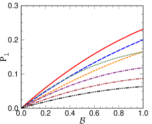
Figure 2: The probability, $P_{l}$, for the atom to leak to the state $|l\rangle$ after one SWAP as a function of the branching ratio, ${\cal B}$, to the leak state. The solid (red) line is for $\tilde{\omega}_{r}=0.25$, the medium dash (blue) line is for 0.35, the short dash (orange) line is for 0.5, the the dotted (green) line is for 0.7, the dash-dot (purple) line is for 1.0, the dash-dot-dot (maroon) line is for 1.4, and the dash-dot-dot-dot (black) line is for 2.0. For all calculations, the atom starts in the ground state with $p=20\hbar k$.

In this section, the initial state has all of the population in one particular momentum state. One sweep is performed. This situation mimics that of slowing a beam of atoms. The quantities of interest are the amount of population lost into state $|l\rangle$ and the change in energy of the states. In all of the calculations, the atom starts in the ground state with $p=20\hbar k$.

There are several parameters that control the population lost into the leak state and the energy removed during the SWAP. We chose to study how the population in the leak state and the final energy varied with the branching ratio, ${\cal B}$, to spontaneously decay to the leak state, $|l\rangle$, for a few scaled recoil frequencies, $\tilde{\omega}_{r}$. The $\tilde{\omega}_{r}$ was stepped by the factor $\sim 1.4$ to show a range of behavior. The range of the sweep, $\Delta_{s}$, was scaled for each $\tilde{\omega_{r}}$ so that $\tilde{\Delta}_{s}=240\tilde{\omega}_{r}$. For each $\tilde{\omega}_{r}$, the $\tilde{\Omega}_{s}$ was varied to give the best slowing for ${\cal B}=0$ and was then fixed for all other values of the branching ratio. The ramp rate was chosen so that $\alpha=\Omega_{s}^{2}/2$ (i.e. $\kappa=2$) which gives a Landau-Zener probability of $P\simeq 0.96$. A slower ramp rate would give a larger Landau-Zener probability but at the cost of spontaneous emission between the stimulated absorption and stimulated emission steps. After the SWAP, the excited state population was allowed to decay as in Ref. Bartolotta et al. (2018).

The parameters in the simulation gave a final energy after one SWAP that ranged from $0.82\times$ the initial energy for $\tilde{\omega}_{r}=2$ to $0.84\times$ the initial energy for $\tilde{\omega}_{r}=0.25$. For a perfect SWAP, the momentum should go from $20\hbar k$ to $18\hbar k$ meaning the expected final energy is $(18/20)^{2}=0.81\times$ that of the initial energy. This indicates that the SWAP procedure is effective at slowing the atoms for $n_{p}\sim 20$, roughly independent of the decay rate. As an example, for $\tilde{\omega}_{r}=1$, 89% of the population finishes in the $18\hbar k$ momentum state when ${\cal B}=0$.

Figure 2 shows the population that leaks to the state $|l\rangle$ as a function of ${\cal B}$. As expected, there is no population leak for ${\cal B}=0$, and the population in $|l\rangle$ increases with the branching ratio. For small branching ratio into the leak state, ${\cal B}$, the leaked population, $P_{l}$, is proportional to ${\cal B}$, but increases slower than linear for larger ${\cal B}$. The slope of $P_{l}$ for ${\cal B}\sim 0$ determines the effectiveness of the SWAP procedure at small branching ratios: smaller slope means less loss and a greater effectiveness. Although the ${\cal B}\sim 0$ is important, even the extreme case ${\cal B}\sim 1$ (i.e. the branching ratio of spontaneous emission into the leak state is $\sim$100%), has less than 1/4 of the population leaking into state $|l\rangle$ during a SWAP for the parameters in Fig. 2. As an example, for $\tilde{\omega}_{r}=1$, the ${\cal B}\sim 1$ population loss is 12% per sweep. If this loss were the same for successive $n_{p}$, there would be approximately 70% population loss after 10 SWAPs. Similarly, the $\tilde{\omega}_{r}=1$, ${\cal B}=1/2$ case gives 8% loss per SWAP which is a factor of $\simeq 6$ suppression of the loss that would occur for Doppler cooling.

With one exception, there is a clear trend of decreasing population leak as $\tilde{\omega}_{r}$ increases. This is understandable because an increased scaled recoil energy means a smaller decay rate, which should make the SWAP procedure more effective: there is more stimulated emission back to $|g\rangle$ and less spontaneous emission which could lead to either $|g\rangle$ or $|l\rangle$. As an example, the $\tilde{\omega}_{r}=1$ case (dash-dot (purple) line) used $\tilde{\Omega}_{s}=33$ and had $P_{l}\simeq{\cal B}/5$ for ${\cal B}\simeq 0$. For this case, the loss is $\simeq 5\times$ smaller than the best case using Doppler cooling. Even the worst case shown ($\tilde{\omega}_{r}=0.25$ solid (red) line) has a loss for ${\cal B}\simeq 0$ that is $\simeq 3\times$ smaller than the best case using Doppler cooling. The exception to the trend is the $\tilde{\omega}_{r}=0.7$ (dotted (green) line). This case also had an anomalous value for $\tilde{\Omega}_{s}$ compared to the trends observed for the other $\tilde{\omega}_{r}$. We do not know why this case is different from what we expected.

IV.2.2 Thermal distribution

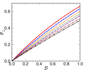
Figure 3: The probability, $P_{l}$, for the atom to leak to the state $|l\rangle$ after one SWAP as a function of the branching ratio, ${\cal B}$, to decay to the leak state, $|l\rangle$. The line types are the same as Fig. 2. For all calculations, the atom starts in a thermal distribution of momenta as described in the text.

In this section, we present the results for the effect of one SWAP when the initial distribution of momenta is thermal. The initial distribution was chosen to be proportional to $\exp(-[n_{p}/14]^{2})$ which corresponds to a temperature, $k_{B}T=98\hbar\omega_{r}$. This temperature was chosen to give similar SWAP parameters to Sec. IV.2.1. As with the previous section, we performed calculations for several $\tilde{\omega}_{r}$, the range of the sweep was $\tilde{\Delta}_{s}=240\tilde{\omega}_{r}$, and we varied the $\tilde{\Omega}_{s}$ for each $\tilde{\omega}_{r}$ to obtain the best cooling for ${\cal B}=0$.

There was not a substantial difference in the amount of energy removed in one SWAP for different $\tilde{\omega}_{r}$ at ${\cal B}=0$. This trend is similar to that in the previous section. The final average energy somewhat increased with decreasing $\tilde{\omega}_{r}$: largest for $\tilde{\omega}_{r}=1/4$ (approximately $0.83\times$ the initial average energy) and smallest for $\tilde{\omega}_{r}=2$ (approximately $0.78\times$ the initial average energy).

The population that leaked to state $|l\rangle$ after one SWAP is plotted in Fig. 3 for several different $\tilde{\omega}_{r}$. The line types are the same as for Fig. 2. The amount of population that leaks out of the cycling transition is much larger than for the previous section where only one momentum component is initially occupied. This is because the thermal distribution has several momentum components, and the SWAP parameters were chosen to give an overall efficiency. However, parameters that work well for large momenta are not so good for small momenta and vice versa. The best slope for small ${\cal B}$ is for $\tilde{\omega}_{r}=2$ and is $\sim 2\times$ smaller than would result from spontaneous emission from the excited state. Unlike the previous section, the interpretation of this slope is ambiguous because it is not clear how many photons were absorbed.

Figure 4: The probability, $P$, for the atom to be in the momentum state $n_{p}\hbar k$. The solid (red) line is the initial momentum distribution. The medium dash (blue) line is the momentum distribution when the atom finishes in the $|g\rangle$ state for $\tilde{\omega}_{r}=1$ and the short dash (orange) line is when the atom finishes in the $|l\rangle$ state. This line has been scaled to give the same area as the medium dash (blue) line. The branching ratio to spontaneously decay back to $|g\rangle$ is $1-{\cal B}=0.99$ for these results.

The momentum distribution after SWAP, Fig. 4, indicates that the atoms that leak into the state $|l\rangle$ are those with smaller energy. In this calculation, $\tilde{\omega}_{r}=1$ and the branching ratio back to $|g\rangle$ is $1-{\cal B}=0.99$. For this case, 0.605% of the atoms leak to the state $|l\rangle$. The solid (red) line shows the initial thermal distribution of the atoms. The medium dash (blue) line shows the momentum distribution after the SWAP for the atoms that finish in the $|g\rangle$ state. The increase in the distribution for small $|n_{p}|$ shows that there has been cooling during the SWAP, even with the loss. The short dash (orange) line is the momentum distribution for atoms that leaked to $|l\rangle$. This distribution has been scaled so the integral would be the same as for the $|g\rangle$ state. This distribution is even more strongly peaked at small $|n_{p}|$ which indicates that the atoms that leak preferentially have smaller energy. This trend is plausible because choosing $\tilde{\Omega}_{s}$ to give the largest energy decrease indicates the SWAP is most efficient for the states with larger $|n_{p}|$.

IV.3 Relative efficiency with loss

Figure 5: The relative SWAP efficiency, $R\equiv(\langle KE\rangle_{0}-\langle KE\rangle_{f})/(\langle KE\rangle_{0}P_{\ell})$ for ${\cal B}=0.02$. One calculation was for a single initial momentum, $20\hbar k$, and the other was for a thermal distribution.

One possible measure of the efficiency of SWAP cooling is the change in energy divided by the population lost to the leak state. In order to make it dimensionless, we define it as $R\equiv(\langle KE\rangle_{0}-\langle KE\rangle_{f})/(\langle KE\rangle_{0}P_{\ell})$. Larger $R$ implies a more effective SWAP either by having a larger change in energy or smaller loss. This quantity is inversely proportional to ${\cal B}$ for small branching ratio to the leak state which leads to the obvious conclusion that smaller loss is better.

Less obvious is the trend with respect to the linewidth keeping the branching ratio small and fixed. Figure 5 shows the results of two calculations of the relative efficiency with ${\cal B}=0.02$ as a function of the scaled recoil frequency, $\tilde{\omega}_{r}$ (smaller decay rate, $\gamma$, means larger $\tilde{\omega}_{r}$). In the left graph, the calculation was performed using the parameters of Fig. 2 (i.e. a specific initial momentum to mimic a beam) while the right graph used parameters of Fig. 3 (i.e. a thermal distribution). To give an idea of the size that might be expected, the beam case would have $R=0.19/0.02=9.5$ for Doppler cooling.

For a given scaled recoil energy, SWAP was more efficient for the beam case than for the thermal case, which is mainly due to the relative slope in Fig. 2 versus 3. For the thermal case, the efficiency monotonically increases with increasing $\tilde{\omega}_{r}$ which supports the proposition that SWAP is better for narrow transitions. However, the increase is not quite as rapid for larger $\tilde{\omega}_{r}$ which indicates there may be limits to the effectiveness of cooling a thermal gas. For the beam, there is a dip in efficiency at $\tilde{\omega}_{r}=0.7$ which matches the increase loss seen in Fig. 2. Otherwise, the trend is an increase in efficiency with increasing $\tilde{\omega}_{r}$ as expected; at $\tilde{\omega}_{r}=2$, the relative efficiency is almost $10\times$ that for Doppler cooling.

IV.4 Implication for $\bar{\rm H}$

One of the motivations for the above studies was to explore whether $\bar{\rm H}$ can be further cooled from the apparent limit of Doppler cooling in the ALPHA trap: the average final energy in the simulation was $\bar{E}_{f}/k_{B}\sim 30$ mKDonnan et al. (2013). This simulation was based on one laser Doppler cooling on the 1S-2P transition at 121.6 nm. The idea for further cooling is to excite the $\bar{\rm H}$ to the metastable 2S state and attempt to laser cool on the 2S-3P or 2S-4P transition. The best case is the 2S-4P transition which has the larger photon momentum and smaller decay rate, meaning it will have the larger $\tilde{\omega}_{r}$; the value, $\tilde{\omega}_{r}\simeq 0.065$, is smaller than any of the values simulated above. For this transition, the Doppler temperature $T_{D}\simeq 0.31$ mK. Thus, the starting $k_{B}T/(\hbar\omega_{r})$ is $5\times$ that in Fig. 3 assuming $T\sim 20$ mKDonnan et al. (2013). Unfortunately, the branching ratio to leak states is ${\cal B}\simeq 0.88$ for either transition. We simulated multiple SWAPs until all of the population had leaked out of the cycling transition and found a decrease of 16% in the kinetic energy. This is a large decrease considering how unfavorable the conditions (i.e. large branching ratio and large linewidth). However, since populating the 2S state is very difficult, the simulations strongly suggest that SWAP cooling is not worthwhile for further cooling $\bar{\rm H}$.

V Conclusion

Results from simulations of SWAP cooling of a thermal distribution or slowing a beam were presented when a loss channel is present. For the cases investigated, there was not a large difference in the cooling or slowing versus the branching ratio, ${\cal B}$, for spontaneous decay into the leak state(s) for one SWAP, and there was less population lost during one SWAP when slowing a beam compared to cooling a thermal distribution. The population lost to the leak state strongly depended on the branching ratio as well as the spontaneous decay rate of the excited state. For small branching ratios, the population lost to the leak state is proportional to the branching ratio but does not increase as rapidly for larger ${\cal B}$. For the same branching ratio, atoms with larger scaled recoil energy, $\varepsilon_{r}/(\hbar\gamma)$, have less population lost into the leak during each SWAP. For the cases we investigated, the population lost during each SWAP for small ${\cal B}$ was as much as $5\times$ smaller than would be lost during Doppler cooling. This confirms the suggestion in Ref. Norcia et al. (2018) that SWAP could be useful for cooling molecules. SWAP might be useful for slowing beams even for unfavorable (i.e. large) branching ratios out of the cycling transition if the scaled recoil energy is large.

This work was partially supported by NSF REU grant PHY-1852501 (JG and MEP) and NSF grant PHY-1806380 (JG, MEP, and FR).

References

- Metcalf and van der Straten (1999) H. J. Metcalf and P. van der Straten, Laser Cooling and Trapping (Springer, 1999).
- Foot (2005) C. J. Foot, Classical Electrodynamics, 3rd Edition (Oxford University Press, 2005).
- Carr et al. (2009) L. D. Carr, D. DeMille, R. V. Krems, and J. Ye, “Cold and ultracold molecules: science, technology and applications,” New J. Phys. 11, 055049 (2009).
- Novotny and Hecht (2012) L. Novotny and B. Hecht, Principles of nano-optics (Cambridge University Press, 2012).
- Norcia et al. (2018) M. A. Norcia, J. R. K. Cline, J. P. Bartolotta, M. J. Holland, and J. K. Thompson, “Narrow-line laser cooling by adiabatic transfer,” New J. Phys. 20, 023021 (2018).
- Bartolotta et al. (2018) J. P. Bartolotta, M. A. Norcia, J. R. K. Cline, J. K. Thompson, and M. J. Holland, “Laser cooling by sawtooth-wave adiabatic passage,” Phys. Rev. A 98, 023404 (2018).
- Petersen et al. (2019) N. Petersen, F. Mühlbauer, L. Bougas, A. Sharma, D. Budker, and P. Windpassinger, “Sawtooth-wave adiabatic-passage slowing of dysprosium,” Phys. Rev. A 99, 063414 (2019).
- Snigirev et al. (2019) S. Snigirev, A. J. Park, A. Heinz, I. Bloch, and S. Blatt, “Fast and dense magneto-optical traps for strontium,” Phys. Rev. A 99, 063421 (2019).
- Liang et al. (2019) Q. Liang, T. Chen, W. Bu, Y. Zhang, and B. Yan, “Laser cooling with adiabatic passage for diatomic molecules,” arXiv preprint arXiv:1902.05212 (2019).
- Donnan et al. (2013) P. H. Donnan, M. C. Fujiwara, and F. Robicheaux, “A proposal for laser cooling antihydrogen atoms,” J. Phys. B 46, 025302 (2013).
- Ahmadi and et al (ALPHA collaboration) M Ahmadi and et al (ALPHA collaboration), “Characterization of the 1s–2s transition in antihydrogen,” Nature 557, 71 (2018).