Cross-Validation,
Risk Estimation, and Model Selection

Abstract

Cross-validation is a popular non-parametric method for evaluating the accuracy of a predictive rule. The usefulness of cross-validation depends on the task we want to employ it for. In this note, I discuss a simple non-parametric setting, and find that cross-validation is asymptotically uninformative about the expected test error of any given predictive rule, but allows for asymptotically consistent model selection. The reason for this phenomenon is that the leading-order error term of cross-validation doesn’t depend on the model being evaluated, and so cancels out when we compare two models. This note was prepared as a comment on a paper by Rosset and Tibshirani, forthcoming in the Journal of the American Statistical Association.

How best to estimate the accuracy of a predictive rule has been a longstanding question in statistics. Approaches to this task range from simple methods like Mallow’s Cp to algorithmic techniques like cross-validation; see Arlot and Celisse (2010), Efron (1983, 2004), Hastie, Tibshirani, and Friedman (2009), Mallows (1973), and references therein. Rosset and Tibshirani (2019) contribute to this discussion by considering how some classical results on the “optimism” of the apparent error of a predictive rule, i.e., the amount by which the training set error of a fitted statistical predictor is expected to underestimate its test set error, change when we consider a random- versus fixed-$X$ sampling design. This is a welcome addition to the literature as, in modern statistical settings, we often need to work with large observational datasets that were incidentally collected as a by-product of some other task, and in these cases random-$X$ modeling is more appropriate than the classical fixed-$X$ approach.

There are two reasons a statistician may want to estimate the accuracy of a predictive model. One is to simply understand the quality of its predictions: For example, a company may need to choose whether to purchase a new forecasting tool, and want to evaluate its accuracy in order to better understand the value of the tool for its business. Another motivation is model selection: Cross-validation and related methods are often used to choose between competing predictive rules, or to set the complexity parameter with methods like the lasso (Chetverikov, Liao, and Chernozhukov, 2016; Hastie, Tibshirani, and Friedman, 2009). For the first task, we in fact need to accurately estimate the accuracy of the predictive rule itself, and the results of Rosset and Tibshirani (2019) are focused on this task. For the second, however, we only need to compare the accuracy of two competing rules; and this statistical task ends up having fairly different properties than risk estimation.

In this note, I compare properties of $K$-fold cross-validation for both risk estimation and model comparison under random-$X$ asymptotics. We have access to independent and identically distributed samples $(X_{i},\,Y_{i})\in\mathcal{X}\times\mathbb{R}$, and want to predict $Y_{i}$ from $X_{i}$ under squared error loss. The optimal predictive rule is the conditional response function $\mu(x)=\mathbb{E}\left[Y\,\big{|}\,X=x\right]$. For simplicity, I’ll focus on evaluating models $\hat{\mu}(x)$ whose root-mean-squared excess error $\mathbb{E}[(\hat{\mu}(X)-\mu(X))^{2}]^{1/2}$ decays with sample size $n$ as $n^{-\gamma}$, for some exponent $1/4<\gamma<1/2$. In other words, I assume that the predictor converges slower than the parametric $1/\sqrt{n}$ rate, but faster than the $1/\sqrt[4]{n}$.

In this setting, cross-validation is asymptotically uninformative about the test set error of the fitted rule in that, as described more formally below, the analyst would prefer to estimate the test-set error of $\hat{\mu}(\cdot)$ as $\operatorname{Err}^{*}=\mathbb{E}[(Y-\mu(X))^{2}]$ (which does not depend on the specific choice of $\hat{\mu}(\cdot)$) than to use cross-validation. Conversely, cross-validation is asymptotically consistent for model selection, i.e., given the choice of two predictors, it repeatedly picks the more accurate of the two.

Thus, whether we should adopt an optimistic or pessimistic view of cross-validation depends largely on the statistical task at hand. I want to emphasize that the result presented here is not new; for example, it is implicit in the proof of Theorem 1 of Yang (2007). The purpose of this discussion is simply to highlight this fact, and to offer a simple argument that applies in the random-$X$ setting of Rosset and Tibshirani (2019).

Numerical example

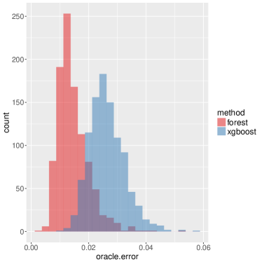
$\text{avg}_{\text{test}}\left[\left(\mu(X_{i})-\hat{\mu}(X_{i})\right)^{2}\right]$	$\text{avg}_{\text{train}}\left[\left(Y_{i}-\hat{\mu}^{(-i)}(X_{i})\right)^{2}\right]$

Figure 1: Comparison of the performance of boosting and regression forests on the data-generating process (1), both in terms of test set excess mean-squared error and training set cross-validation error. The numbers are aggregated across 1000 simulation replications.

Before a more formal discussion, consider the following simulation example. We generate data as

$$X\sim\mathcal{N}\left(0,\,\mathcal{I}_{p\times p}\right),\ \ Y\,\big{|}\,X\sim\mathcal{N}\left(\mu(X),\,1\right),\ \ \mu(x)=\frac{1\left(\left\{x_{1}>0\right\}\right)}{1+e^{-2x_{2}}},$$ (1)

with $p=10$ and $n=1,600$. We then seek to fit this signal using gradient boosting as implemented in xgboost (Chen and Guestrin, 2016) and regression forests as implemented in grf (Athey, Tibshirani, and Wager, 2019), both with built-in parameter tuning. We compare the methods via cross-validation. For boosting, we use 10-fold cross-validation, whereas for forests we use leave-one-out (or out-of-bag) evaluation (Breiman, 2001).

As shown in the left panel of Figure 1, forests are noticeably more accurate for this task than boosting. However, as seen in the right panel, the marginal distribution of the cross-validated errors of forests versus boosting are nearly indistinguishable. Thus, at first glance, Figure 1 appears to paint a fairly bleak picture: Forests are more accurate than boosting here, but cross-validation cannot tell the difference.

As shown in Figure 2, however, the picture clears up when we take differences. As shown in the left panel of Figure 2, cross-validation consistently picks the more accurate method here. Accurate model selection is possible despite the finding from Figure 1 because, as shown in the right panel of Figure 2, the cross-validated error estimates for forests and boosting are highly correlated, and this shared noise component cancels out when we take a difference.

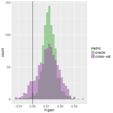
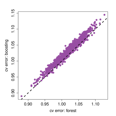
Figure 2: In the setting of Figure 1, comparison of the cross-validation errors of boosting and forests within a single simulation replication. The left panel shows a histogram of the cross-validation error of the forest minus the cross-validation error of boosting across the 1000 simulation replications. The overlaid “oracle” histogram shows the difference in test set errors (i.e., differences of the quantities whose marginal histograms are shown in the left panel of Figure 1). The right panel shows the same information in a scatter plot.

Formal results

Cross-validation is used to evaluate an algorithm $A$ that takes a set of $n$ training samples and turns them into an rule $\hat{\mu}(\cdot)$ that predicts $Y_{i}$ from $X_{i}$, i.e.,

$$A:\cup_{n=1}^{\infty}\left\{\mathcal{X}\times\mathbb{R}\right\}^{n}\rightarrow\left\{\mathcal{X}\rightarrow\mathbb{R}\right\},\ \ \ \ A\left(\left\{(X_{i},\,Y_{i})\right\}_{i=1}^{n}\right)=\hat{\mu}(\cdot).$$ (2)

Some papers use common notation to denote both the algorithm $A$ and the fitted predictor $\hat{\mu}(\cdot)$; here, however, it’s helpful to disambiguate notation so that we can be specific about our assumptions. Throughout, we consider cross-validation as a tool for evaluating the algorithm $A$, rather than the actual predictive rule $\hat{\mu}(\cdot)$ that was obtained using the training data.

Given this notation, $K$-fold cross-validation operates as follows. Start with a set of $n$ training samples, and divide them into $K$ evenly sized and non-overlapping folds $\mathcal{S}_{1},\,...,\,\mathcal{S}_{K}$. Then, for each $k=1,\,...,\,K$, run the algorithm $A$ on data in all but the $k$-th fold to obtain $\hat{\mu}^{(-k)}(\cdot)$. The estimate of the error of $A$ when trained on $n$ samples is then

$$\widehat{\operatorname{CV}}_{n,K}\left(A\right)=\frac{1}{n}\sum_{k=1}^{K}\sum_{i\in\mathcal{S}_{k}}\left(Y_{i}-\hat{\mu}^{(-k)}(X_{i})\right)^{2}.$$ (3)

Throughout, we assume that the method $A$ yields a predictor $\hat{\mu}(\cdot)$ whose root-mean squared excess test error scales as $n^{-\gamma}$ conditionally on the training data. This type of behavior can be verified, e.g., for kernel smoothing or local linear regression when $\mu(\cdot)$ satisfies reasonable regularity conditions.

Assumption 1.

We have access to a stream independent and identically distributed samples $(X_{i},\,Y_{i})\in\mathcal{X}\times\mathbb{R}$ with $\mathbb{E}\left[Y^{4}\right]\leq\infty$ and $\operatorname{Var}\left[Y_{i}\,\big{|}\,X_{i}\right]\leq\Omega$. We also have an algorithm $A$ for learning predictors $\hat{\mu}(\cdot)$ with the following property. There are constants $0<C_{-}\leq C_{+}<\infty$ and $0.25<\gamma<0.5$ such that, when trained on $n$ samples $\left\{(X_{i},\,Y_{i})\right\}_{i=1}^{n}$, the excess risk of $\hat{\mu}(\cdot)$ scales as

$$\begin{split}&\lim_{n\rightarrow\infty}\mathbb{P}\left[n^{\gamma}\,\mathbb{E}\left[\left(\hat{\mu}(X)-\mu(X)\right)^{2}\,\big{|}\,\left\{(X_{i},\,Y_{i})\right\}_{i=1}^{n}\right]^{\frac{1}{2}}\leq C_{-}\right]=0,\\ &\lim_{n\rightarrow\infty}\mathbb{P}\left[n^{\gamma}\,\mathbb{E}\left[\left(\hat{\mu}(X)-\mu(X)\right)^{2}\,\big{|}\,\left\{(X_{i},\,Y_{i})\right\}_{i=1}^{n}\right]^{\frac{1}{2}}\leq C_{+}\right]=1,\end{split}$$ (4)

where $X$ denotes a test sample drawn independently from the training distribution.

To study the behavior of cross-validation under this assumption, it is helpful to expand-out the square, as is done in Rosset and Tibshirani (2019), Yang (2007), etc.:

$$\widehat{\operatorname{CV}}_{n,K}\left(A\right)=\widehat{\operatorname{CV}}^{*}_{n,K}+2Z_{n,K}\left(A\right)+\Delta^{2}_{n,K}\left(A\right),\ \text{ where }$$

$$\widehat{\operatorname{CV}}^{*}_{n,K}=\frac{1}{n}\sum_{i=1}^{n}\left(Y_{i}-\mu(X_{i})\right)^{2},\ \ \ \ \Delta^{2}_{n,K}\left(A\right)=\frac{1}{n}\sum_{k=1}^{K}\sum_{i\in\mathcal{S}_{k}}\left(\mu(X_{i})-\hat{\mu}^{(-k)}(X_{i})\right)^{2},$$

$$Z_{n,K}\left(A\right)=\frac{1}{n}\sum_{k=1}^{K}\sum_{i\in\mathcal{S}_{k}}\left(Y_{i}-\mu(X_{i})\right)\left(\mu(X_{i})-\hat{\mu}^{(-k)}(X_{i})\right).$$

In other words, $\widehat{\operatorname{CV}}^{*}_{n,K}$ is the training set error of the optimal predictor $\hat{\mu}(\cdot)$, $\Delta^{2}_{n,K}(A)$ is an oracle estimate of the excess error of the fitted rule, and $Z_{n,K}(A)$ is a cross-term.

Given this decomposition, we note that

$$\sqrt{n}\left(\widehat{\operatorname{CV}}^{*}_{n,K}-\operatorname{Err}^{*}\right)\Rightarrow\mathcal{N}\left(0,\,\operatorname{Var}\left[\left(Y-\mu(X)\right)^{2}\right]\right),\ \ \operatorname{Err}^{*}=\mathbb{E}\left[\left(Y-\mu(X)\right)^{2}\right].$$ (5)

Meanwhile, by our cross-fold construction, we can verify that $\mathbb{E}\left[Y_{i}-\mu(X_{i})\,\big{|}\,X_{i},\,\hat{\mu}^{(-k)}(X_{i})\right]=0$ for all $i\in\mathcal{S}_{k}$, and furthermore that $Y_{i}-\mu(X_{i})$ and $Y_{j}-\mu(X_{j})$ are pairwise uncorrelated for $i,\,j\in\mathcal{S}_{k}$ conditionally on $\hat{\mu}^{(-k)}(X_{i})$. The upshot is that, by Assumption 1, for all $k=1,\,...,\,K$

$$\mathbb{E}\left[\sum_{i\in\mathcal{S}_{k}}\left(Y_{i}-\mu(X_{i})\right)\left(\mu(X_{i})-\hat{\mu}^{(-k)}(X_{i})\right)\,\big{|}\,\hat{\mu}^{(-k)}(\cdot)\right]=0\text{ and }$$

$$\mathbb{P}\left[\frac{n_{k}^{2\gamma}}{\left\lvert\mathcal{S}_{K}\right\rvert}\mathbb{E}\left[\left(\sum_{i\in\mathcal{S}_{k}}\left(Y_{i}-\mu(X_{i})\right)\left(\mu(X_{i})-\hat{\mu}^{(-k)}(X_{i})\right)\right)^{2}\,\big{|}\,\hat{\mu}^{(-k)}(\cdot)\right]\leq C^{2}_{+}\,\Omega\right]=1,$$

where $n_{k}=n-\left\lvert\mathcal{S}_{k}\right\rvert$ denotes the amount of training data available to learn $\hat{\mu}^{(-k)}$. Thus, by Markov’s inequality,

$$Z_{n,K}\left(A\right)=\mathcal{O}_{p}\left(\frac{1}{n^{0.5+\gamma}}\right).$$ (6)

Finally, given the scaling in Assumption 1, the oracle mean-squared excess risk $\Delta^{2}_{n,K}(A)$ scales as $n^{-2\gamma}$ in probability.

A first immediate consequence of this decomposition is that, to first order, the cross-validated error estimate of $A$ depends only on the test-set error of the optimal predictor $\mu(\cdot)$, and $\widehat{\operatorname{CV}}_{n,K}\left(A\right)$ is asymptotically equivalent to $\widehat{\operatorname{CV}}^{*}_{n,K}$. Thus, an analyst wanting to estimate the expected test set error of $\hat{\mu}(\cdot)$, i.e., $\mathbb{E}[(Y-\hat{\mu}(X))^{2}\,\big{|}\,\left\{(X_{i},\,Y_{i})\right\}_{i=1}^{n}]$, under mean squared error would prefer to use a point estimate $\operatorname{Err}^{*}=\mathbb{E}[(Y-\mu(X))^{2}]$ (which does not depend on $\hat{\mu}$) than to use cross-validation.

Proposition 1.

Under Assumption 1, the first-order behavior of $\widehat{\operatorname{CV}}_{n,K}\left(A\right)$ does not depend on the method $A$ being evaluated:

$$\sqrt{n}\left(\widehat{\operatorname{CV}}_{n,K}\left(A\right)-\operatorname{Err}^{*}\right)\Rightarrow\mathcal{N}\left(0,\,\operatorname{Var}\left[\left(Y-\mu(X)\right)^{2}\right]\right).$$ (7)

The picture becomes more encouraging, however, when we seek to use cross validation to compare two different predictive rules. The dominant source of noise $\widehat{\operatorname{CV}}^{*}_{n,K}$ underlying the result in Proposition 1 does not depend on $A$, and so cancels out when we compare two rules. Meanwhile, the cross-term $Z_{n,K}\left(A\right)$ decays faster than the oracle excess error term $\Delta^{2}_{n,K}\left(A\right)$, meaning that cross-validation allows for asymptotically perfect model selection.

Proposition 2.

Suppose we have two methods $A$ and $A^{\prime}$ satisfying 1 with constants $(\gamma,\,C_{-},\,C_{+})$ and $(\gamma^{\prime},\,C_{-}^{\prime},\,C_{+}^{\prime})$ respectively. Suppose moreover that $\gamma>\gamma^{\prime}$, or that $\gamma=\gamma^{\prime}$ and $C_{+}<C_{-}^{\prime}$. Then,

$$\frac{\widehat{\operatorname{CV}}_{n,K}\left(A^{\prime}\right)-\widehat{\operatorname{CV}}_{n,K}\left(A\right)}{\Delta^{2}_{n,K}\left(A^{\prime}\right)-\Delta^{2}_{n,K}\left(A\right)}\rightarrow_{p}1,$$ (8)

and $\lim_{n\rightarrow\infty}\mathbb{P}\left[\widehat{\operatorname{CV}}_{n,K}\left(A^{\prime}\right)>\widehat{\operatorname{CV}}_{n,K}\left(A\right)\right]=1$.

Together, Propositions 1 and 2 mean that, given two methods for generating predictive rules that satisfy Assumption 1, the prima facie risk estimates provided by cross-validation are asymptotically independent of the methods being evaluated, but model selection via cross-validation can accurately pick the better of the two methods. Returning to our numerical example presented above, one could argue that Proposition 1 predicts the indistinguishability of the two histograms as observed in the right panel of Figure 1, whereas Proposition 2 helps explain the success of model selection witnessed in Figure 2.

Estimating the error rate of a prediction rule is an important statistical task, and Rosset and Tibshirani (2019) contribute valuable new results to this endeavor in the case of random-$X$ asymptotics. In studying the properties of cross-validation, though, results are qualitatively different when we focus on model evaluation versus model comparison. This is not only a formal curiosity, but also affects how we interpret cross-validation in practical examples; see, e.g., the discussion in Section 2.1 of Nie and Wager (2017). Related facts are also reflected in statistical practice through, e.g., the recommendation to use McNemar’s test to compare the accuracy of two classification rules, or in using a consensus test-train split for evaluating methods in shared engineering tasks. It would be interesting to see whether the results of Rosset and Tibshirani (2019) on optimism allow for natural extension to the case of model comparison.

References

- Arlot and Celisse [2010] Sylvain Arlot and Alain Celisse. A survey of cross-validation procedures for model selection. Statistics Surveys, 4:40–79, 2010.
- Athey et al. [2019] Susan Athey, Julie Tibshirani, and Stefan Wager. Generalized random forests. The Annals of Statistics, 47(2):1148–1178, 2019.
- Breiman [2001] Leo Breiman. Random forests. Machine learning, 45(1):5–32, 2001.
- Chen and Guestrin [2016] Tianqi Chen and Carlos Guestrin. Xgboost: A scalable tree boosting system. In Proceedings of the 22nd ACM SIGKDD International Conference on Knowledge Discovery and Data Mining, pages 785–794. ACM, 2016.
- Chetverikov et al. [2016] Denis Chetverikov, Zhipeng Liao, and Victor Chernozhukov. On cross-validated lasso. arXiv preprint arXiv:1605.02214, 2016.
- Efron [1983] Bradley Efron. Estimating the error rate of a prediction rule: improvement on cross-validation. Journal of the American Statistical Association, 78(382):316–331, 1983.
- Efron [2004] Bradley Efron. The estimation of prediction error: covariance penalties and cross-validation. Journal of the American Statistical Association, 99(467):619–632, 2004.
- Hastie et al. [2009] Trevor Hastie, Robert Tibshirani, and Jerome Friedman. The Elements of Statistical Learning: Data Mining, Inference, and Prediction. Springer Science & Business Media, 2009.
- Mallows [1973] Colin L Mallows. Some comments on Cp. Technometrics, 15(4):661–675, 1973.
- Nie and Wager [2017] Xinkun Nie and Stefan Wager. Quasi-oracle estimation of heterogeneous treatment effects. arXiv preprint arXiv:1712.04912, 2017.
- Rosset and Tibshirani [2019] Saharon Rosset and Ryan J Tibshirani. From fixed-X to random-X regression: Bias-variance decompositions, covariance penalties, and prediction error estimation. Journal of the American Statistical Association, forthcoming, 2019.
- Yang [2007] Yuhong Yang. Consistency of cross validation for comparing regression procedures. The Annals of Statistics, 35(6):2450–2473, 2007.