Comment on ‘Fluctuation-dominated phase ordering at a mixed order transition’
Abstract
Renewal processes generated by a power-law distribution of intervals with tail index less than unity are genuinely non-stationary. This issue is illustrated by a critical review of the recent paper by Barma, Majumdar and Mukamel 2019 J. Phys. A 52 254001, devoted to the investigation of the properties of a specific one-dimensional equilibrium spin system with long-range interactions. We explain why discarding the non-stationarity of the process underlying the model leads to an incorrect expression of the critical spin-spin correlation function, even when the system, subjected to periodic boundary conditions, is translation invariant.
1 Introduction
Reference [1] revisits the tidsi model, a truncated version of a microscopic one-dimensional spin model with long-range interactions, dubbed the inverse distance squared Ising (idsi) model [2, 3, 4]. This tidsi model, which has been investigated in a series of papers in recent years [5, 6, 7], is made of a fluctuating number of domains, filling up the total size of the system. A configuration is thus entirely specified by the number and sizes of these domains. The Boltzmann weight associated to the realisation of such a configuration reads [1]
| (1.1) |
where the denominator is the partition function
| (1.2) |
which ensures the normalisation, and is the Kronecker delta. In (1.1), denotes the fugacity and is given by
| (1.3) |
where , and the tail index is positive. In [1, 5, 6] the phase diagram is analysed according to the values of the fugacity and the index , which are the two parameters of the model. For , such that
| (1.4) |
where is the Riemann zeta function, the system is critical, separating a paramagnetic (disordered) phase from a ferromagnetic (ordered) one.
The main goal of [1] is to obtain the expression of the critical correlation function between two spins located at and , in the regime of short separations, i.e., where the separation between the two points is small compared to the system size (), when the tail index . The expression derived in [1] is
| (1.5) |
As argued in [1], this expression is independent of the position of the first spin and only depends on the separation , because periodic boundary conditions are chosen, which makes the system translation invariant.
The principal aim of this Comment it to show that, in the present context where , the method used in [1] in order to derive (1.5)—the so-called independent interval approximation—does not lead to exact results, as claimed in this reference, and can only predict the scaling behaviour but not the amplitude 111Another method, similar in spirit, is also presented in [1], and leads again to the same result (1.5).. We shall also compare the study made in [1] to the existing literature on the subject. In this respect, we start by disproving an assertion made in [1], which contradicts a statement made in [8, 9].
2 The class of tied-down renewal processes
As stated in [8, 9], the tidsi model defined by (1.1), (1.2), (1.3) belongs to the class of tied-down renewal processes (independently of any considerations on the boundary conditions).
This can be very simply seen by introducing the parameter and making the change of notations
| (2.1) |
Now (1.1) and (1.2) respectively read
| (2.2) |
and
| (2.3) |
Equation (2.2) is nothing but the joint distribution for the class of tied-down renewal processes with a penalty or reward parameter (see [10] and references therein). For this class of processes, a configuration is specified by a fluctuating number of intervals (e.g., domains) which are independent and identically distributed (iid) random variables with common probability distribution
| (2.4) |
A realisation of such a configuration, where the number of intervals takes the value and the random variables take the values , has weight (2.2). These processes are renewal processes because the intervals are iid random variables, and they are tied down because these intervals are conditioned to sum up to a given value , generalising the tied-down random walk, starting from the origin and conditioned to end at the origin at a given time [11, 9]. (For the tied-down random walk, intervals are temporal, while in the rest of this Comment all intervals are spatial.) The definitions (2.2), (2.3) and (2.4) easily generalise to the case where intervals are continuous random variables.
The parameter is larger than 1 in the disordered phase, equal to 1 at criticality, and less than 1 in the ordered phase. The very same model—as defined by (1.1), (1.2) and (1.3)—was already introduced in [12], where the phase diagram of the model was discussed.
The class of tied-down renewal processes defined by (2.2), (2.3) and (2.4) above, encompasses as a particular case the model defined in [12] and [1, 5, 6, 7]. This class itself belongs to the broader class of linear models described in [13], such as the Poland-Scherraga model, wetting models, etc.
To conclude, the following assertion, made in [1], does not hold true: ‘A joint distribution similar to equation (10) was studied in the context of the tied-down renewal process [10], with the important difference that in the latter case the fugacity was taken to be exactly 1. As we will see later, in our tidsi model where can vary, there is a mixed-order phase transition at a critical value (which need not be 1)’222In the first sentence quoted above, equation (10) refers to (2.2), and reference [10] refers to [8].. In these sentences, a confusion is made between the parameter and the fugacity . In the cited work [10] (see the footnote) the parameter taken to 1 is (hence ) and not the fugacity .
From now on, is taken equal to 1, since all the present discussion concerns the critical correlation function. An important consequence of the above is that all results found in [8, 9] hold for the tidsi model. This applies, in particular, to (3.7) and (3.8) in section 3, as already stated in [8, 9].
3 Stationarity and non-stationarity of renewal processes
Let us now give a short reminder of the relevant knowledge on two-space—or two-time—correlation functions in renewal theory, as a preparation for the critical review of [1] given in section 4.
3.1 The correlation function
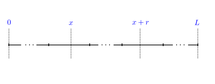
Let be the number of points (events, domain walls, …) comprised between two arbitrary positions and on the line, as depicted in figure 1. The correlation function of interest is by definition
| (3.1) |
where is the probability distribution
| (3.2) |
We are interested in the behaviour of this correlation function when the distribution of intervals is broad, with tail index , and tail parameter ,
| (3.3) |
with emphasis on the case , and when are all simultaneously large. In this regime, as shown in [8], the correlation function is dominated by , the probability that the interval does not contain any point. From now on we shall focus on this quantity. We assume that the first interval begins at site . For the sake of simplicity we use a continuum formalism for the random intervals . In the sequel, we will need the expansion of the Laplace transform of ,
| (3.4) |
where
| (3.5) |
is negative if , positive if , and so on.
3.2 Correlation function for tied-down renewal processes
The correlation function has several regimes according to the respective magnitudes of , , and [8]. Here we restrict the presentation to the regime of short separations, where , which is the only regime considered in [1].
According to the nature of the distribution , the following dichotomy holds [9].
1. finite
If the distribution of intervals has a finite first moment
| (3.6) |
e.g., when is narrow, with finite moments, or broad with a power-law tail of index , then, when , the system enters a stationary regime, where no longer depends on and as can be derived from the analytical expression in Laplace space of this observable [8]. Its asymptotic expression is the same as in the free case and is given in (3.10).
Let us denote by the first moment of the marginal size distribution of a generic interval, , obtained by tracing the full distribution (2.2) on all but one. Alternatively, is equal to the product of by the mean inverse number of intervals in . Then, if , at large , is asymptotically equal to [9].
2. infinite
The situation is different when is a broad distribution with tail index . Then is no longer finite, which is the source of non-stationarity, and [9]
| (3.7) |
where is the tail parameter of the distribution (see (3.3)). In the tidsi model for example, is equal to (see (1.3) and (2.1)).
In the regime of short separations between and (), the correlation function, , has the following expression [8]
| (3.8) | |||||
This expression is non-stationary, since it depends on the ratios and , and universal since it only depends on and no longer on microscopic details of the distribution such as the tail parameter .
3.3 Correlation function for free renewal processes
Now, the correlation function is a function of and only, and we still have for large values of the arguments, with the dependence in dropped out in the notation. The dichotomy seen in the previous subsection still holds.
1. finite
In this situation, in the limit , the process reaches a stationary regime, where (see, e.g., [14, 15]). In Laplace space with respect to , with conjugate variable ,
| (3.9) |
For large, we use the second line of the expansion (3.4) for , which yields, by inversion, the stationary result [15],
| (3.10) |
2. infinite
When is infinite, keeps a dependence in , even at large values of this variable, which is the signature of the non-stationarity of the process [15, 16]. For and simultaneously large and comparable, has the scaling form
| (3.11) |
where the universal scaling function reads [15]
| (3.12) |
In the regime of short separations, (3.11) and (3.12) yield
| (3.13) |
As announced earlier, (3.13) is precisely the limit of (3.8).
4 Derivation of (1.5) in the independent interval approximation
We now come to the derivation of (1.5) given in [1], when , by the so-called independent interval approximation. A similar approach has already been used in [17, 18].
4.1 IIA method
The method, as presented in [1], proceeds as follows.
-
1.
The system is taken infinite ( is sent to infinity), stationary and the distribution of the sizes of domains is assumed to have a finite first moment . Therefore the stationary probability that an interval of size does not contain any point is given by (3.9) in Laplace space, which expresses in terms of the Laplace transform and .
-
2.
In this formalism, is thought as being the marginal , but nevertheless approximated by , if , and is thought as being , and given, according to [1], by
(4.1) which allows to reintroduce in the formalism.
- 3.
4.2 Discussion
According to [1], choosing periodic boundary conditions for the system, entailing translation invariance, justifies the use of a stationary formalism where the dependence in is discarded at the very start, instead of stemming naturally from an analytical computation. In reality, as analysed below, the treatment given in [1] cannot lead to an exact prediction for the correlation function, when .
The range of validity of the IIA method is summarised in point (i) above. If consistently completed—in particular by using the second line of the expansion (3.4) of —it would lead to (3.10) for the correlation function, which has not the expected form . Additional assumptions are therefore introduced in points (ii) and (iii). These assumptions unfortunately do not form a coherent whole. On the one hand, using (3.9) requires to be finite. On the other hand, using the expansion (4.2) only makes sense if is infinite. If is finite one has to use the expansion in the second line of (3.4). Taking in place of does not circumvent this contradiction because the finiteness of is an intrinsic property of the distribution , independent of the size of the system—i.e., holding even for an infinite system. In contrast, is a property of the finite system and depends on .
The IIA method actually does not know about the boundary conditions because it consists of the formal analysis of an infinite system, which can neither take account of a finite size, nor of boundary conditions. This is reflected in the comparison between [1] with the arXiv version [19] of the same work. Except for the change in boundary conditions from open in [19], to periodic in [1], all computations made in [19] remained unchanged, leading to the same result (1.5).
To sum up, the IIA is used in [1] outside its range of validity. It only predicts the power of in (1.5) or (4.3). It has no predictive value for the amplitude in (1.5) or (4.3). All the more as the expression (4.1) for is inaccurate and should be replaced by (3.7). By doing so, the amplitude in (1.5) or (4.3) would be changed to , which does not suffice to give the correct expression for the correlation function either.
5 The role of boundary conditions
To the three possible geometries,
-
1.
the infinite line,
-
2.
the finite system of length as in figure 1,
-
3.
the circle of length ,
correspond three different expressions of the correlation function, assuming .
For the infinite line, the result is given by (3.13) in the short-separation regime (which is the only regime discussed in [1] and in this Comment). For the finite system of length , the result is given by (3.8). These expressions are asymptotic estimates of exact results [15, 8].
Remains to predict an expression for the last case (iii). The question boils down to finding the probability that an interval of size located anywhere on a circle of length contains zero point. If the interval is , since can be anywhere between 0 and , i.e., is uniformly distributed on the circle, one has to integrate uniformly upon this variable the expression (3.8) of the probability that there is zero point in the interval . One thus obtains
| (5.1) |
6 Conclusion
Tied-down renewal processes generated by a power-law distribution of intervals with tail index , of which the critical tidsi model (a spin model with long-range order) is a particular example, are genuinely non-stationary. For such processes, the independent interval approximation put forward in [1] for the computation of the spin-spin correlation function is not the proper approach, because it is applied outside its range of validity and is based on the formal analysis of an infinite system which can neither handle a finite system, nor boundary conditions. When periodic boundary conditions are imposed on the system, entailing translation invariance, the correlation function of the system is obtained by tracing the non-stationary correlation function uniformly on , resulting in (5.1).
References
References
- [1] Barma M, Majumdar S N and Mukamel D 2019 J. Phys. A 52 254001
- [2] Thouless D 1969 Phys. Rev. 187 732
- [3] Anderson P W, Yuval G and Hamann D 1970 Phys. Rev. B 1 4464
- [4] Aizenman M, Chayes J, Chayes L and Newman C 1988 J. Stat. Phys. 50 1
- [5] Bar A and Mukamel D 2014 Phys. Rev. Lett. 112 015701
- [6] Bar A and Mukamel D 2014 J. Stat. Mech. P11001
- [7] Bar A, Majumdar S N, Schehr G and Mukamel D 2016 Phys. Rev. 93 052130
- [8] Godrèche C 2017 J. Stat. Mech. P073205
- [9] Godrèche C 2017 J. Phys. A 50 195003
- [10] Godrèche C 2020 arXiv:2006.04076 [cond-mat.stat-mech] J. Stat. Phys. at press
- [11] Wendel J G 1964 Math. Scand. 14 21
- [12] Bialas P, Burda Z and Johnston D 1999 Nucl. Phys. B 542 413
- [13] Fisher M 1984 J. Stat. Phys. 34 667
- [14] Cox DR 1962 Renewal theory (London: Methuen)
- [15] Godrèche C and Luck J M 2001 J. Stat. Phys. 104 489
- [16] Bouchaud J P and Dean D S 1995 J. Phys. France 5 265
- [17] Das D and Barma M 2000 Phys. Rev. Lett. 85 1602
- [18] Das D, Barma M and Majumdar S N 2001 Phys. Rev. E 64 046126
- [19] Barma M, Majumdar S N and Mukamel D 2019 arXiv:1902.06416v1 [cond-mat.stat-mech]
- [20] Godrèche C 2019 arXiv:1909.11540 [cond-mat.stat-mech]
- [21] Godrèche C in preparation