A numerical method for computing Hadamard finite-part integrals with a non-integral power singularity at an endpoint

Abstract

In this paper, we propose a numerical method of computing a Hadamard finite-part integral with a non-integral power singularity at an endpoint, that is, a finite part of a divergent integral as a limiting procedure. In the proposed method, we express the desired finite-part integral using a complex loop integral, and obtain the finite-part integral by evaluating the complex integral by the trapezoidal formula. Theoretical error estimate and some numerical examples show the effectiveness of the proposed method.

1 Introduction

The integral

$$\int_{0}^{1}x^{\alpha-2}f(x)\mathrm{d}x\quad(\>0<\alpha<1\>),$$

where $f(x)$ is an analytic function on the closed interval $[0,1]$, is divergent. However, we can assign a finite value to this divergent integral as follows. For $0<\epsilon<1$, using integration by part, we have

$$\int_{\epsilon}^{1}x^{\alpha-2}f(x)\mathrm{d}x=\> \frac{1}{\alpha-1}\int_{\epsilon}^{1}(x^{\alpha-1})^{\prime}f(x)\mathrm{d}x$$

$$=\> \frac{1}{\alpha-1}\bigg{[}x^{\alpha-1}f(x)\bigg{]}_{\epsilon}^{1}-\int_{\epsilon}^{1}x^{\alpha-1}f^{\prime}(x)\mathrm{d}x$$

$$=\> \frac{\epsilon^{\alpha-1}f(\epsilon)-f(1)}{1-\alpha}-\int_{\epsilon}^{1}x^{\alpha-1}f^{\prime}(x)\mathrm{d}x$$

$$=\> \frac{\epsilon^{\alpha-1}f(0)}{1-\alpha}+\mbox{(terms finite as $\epsilon\downarrow 0$)},$$

and the limit

$$\lim_{\epsilon\downarrow 0}\left\{\int_{\epsilon}^{1}x^{\alpha-2}f(x)\mathrm{d}x-\frac{\epsilon^{\alpha-1}f(0)}{1-\alpha}\right\}$$

is finite. We call this limit an Hadamard finite-part (f.p.) integral and denote it by

$$\operatorname{f.p.}\int_{0}^{1}x^{\alpha-2}f(x)\mathrm{d}x.$$

Similarly, we can define a f.p. integral

$$\operatorname{f.p.}\int_{0}^{1}x^{\alpha-1-n}f(x)\mathrm{d}x$$ (1)

for $n=1,2,\ldots$, $0<\alpha<1$ and an analytic function $f(x)$ on $[0,1]$ [6].

In this paper, we propose a numerical method of computing f.p. integrals (1). In the proposed method, we express the f.p. integral using a complex loop integral, and we obtain the desired f.p. integral by evaluating the complex integral by the trapezoidal formula with equal mesh. Theoretical error estimate and numerical examples will show that the approximation by the proposed method converges exponentially as the number of sampling points increases.

Previous works related to this paper are as follows. The author and Hirayama proposed a numerical integration method for ordinary integrals related to hyperfunction theory [9], where a desired integral is expressed using a complex loop integral, and it is obtained by evaluating the complex integral by the trapezoidal formula with equal mesh. The author proposed a numerical method of computing f.p. integrals with an integral order singularity [8]. For Cauchy principal value integrals and Hadamard finite-part integrals with a singularity in the interior of the integral interval

$$\operatorname{f.p.}\int_{0}^{1}\frac{f(x)}{(x-\lambda)^{n}}\mathrm{d}x\quad(\>0<\lambda<1,\>n=1,2,\ldots\>),$$ (2)

many numerical methods were proposed. Elliot and Paget proposed a Gauss-type numerical integration formulas for f.p. integrals (2) [5, 11]. Bialecki proposed Sinc numerical integration formulas for f.p. integrals [2, 3], where the trapezoidal formula with the variable transform technique are used as in the DE formula for ordinary integrals [12]. The author et al. improved them and proposed a DE-type numerical integration formulas for f.p. integrals (2) [10].

The remainder of this paper is structured as follows. In Section 2, we define the f.p. integrals and propose a numerical method of computing them. Then, we give a theorem on error estimate of the proposed method. In Section 3, we show some numerical examples which show the effectiveness of the proposed method. In Section 4, we give a summary of this paper.

2 Hadamard finite-part integral

The Hadamard finite-part integral is defined by

$$\operatorname{f.p.}\int_{0}^{1}x^{\alpha-1-n}f(x)\mathrm{d}x=\lim_{\epsilon\downarrow 0}\left\{\int_{\epsilon}^{1}x^{\alpha-1-n}f(x)\mathrm{d}x-\sum_{k=0}^{n-1}\frac{\epsilon^{\alpha-n+k}}{k!(n-k-\alpha)}f^{(k)}(0)\right\}\\ (\>n=1,2,\ldots;\>0<\alpha<1\>).$$ (3)

We can see that it is well-defined using integration by part. In fact, repeating integration by part, we have

$$\int_{\epsilon}^{1}x^{\alpha-n-1}f(x)\mathrm{d}x$$

$$=\> \frac{\epsilon^{\alpha-n}}{n-\alpha}f(\epsilon)+\frac{\epsilon^{\alpha-n+1}}{(n-\alpha)(n-1-\alpha)}f^{\prime}(\epsilon)+\frac{\epsilon^{\alpha-n+2}}{(n-\alpha)(n-1-\alpha)(n-2-\alpha)}f^{\prime\prime}(\epsilon)$$

$$+\cdots+\frac{\epsilon^{\alpha-1}}{(n-\alpha)(n-1-\alpha)(n-2-\alpha)\cdots(1-\alpha)}f^{(n-1)}(0)$$

$$+\frac{1}{(n-\alpha)(n-1-\alpha)(n-2-\alpha)\cdots(1-\alpha)}\int_{\epsilon}^{1}x^{\alpha-1}f^{(n)}(x)\mathrm{d}x$$

$$+\mbox{(terms finite as $n\downarrow 0$, which will be denoted by ``$\cdots$'' below)}$$

$$=\> \frac{\epsilon^{\alpha-n}}{n-\alpha}\sum_{k=0}^{n-1}\frac{\epsilon^{k}}{k!}f^{(k)}(0)+\frac{\epsilon^{\alpha-n+1}}{(n-\alpha)(n-1-\alpha)}\sum_{k=0}^{n-2}\frac{\epsilon^{k}}{k!}f^{(k)}(0)$$

$$+\frac{\epsilon^{\alpha-n+2}}{(n-\alpha)(n-1-\alpha)(n-2-\alpha)}\sum_{k=0}^{n-3}\frac{\epsilon^{k}}{k!}f^{(k)}(0)$$

$$+\cdots+\frac{\epsilon^{\alpha-1}}{(n-\alpha)(n-1-\alpha)(n-2-\alpha)\cdots(1-\alpha)}f^{(n-1)}(0)+\cdots$$

$$=\> \frac{\epsilon^{\alpha-n}}{n-\alpha}f(0)+\frac{\epsilon^{\alpha-n+1}}{n-\alpha}\left(1+\frac{1}{n-1-\alpha}\right)f^{\prime}(0)$$

$$+\frac{\epsilon^{\alpha-n+2}}{n-\alpha}\left\{\frac{1}{2!}+\frac{1}{n-1-\alpha}+\frac{1}{(n-1-\alpha)(n-2-\alpha)}\right\}f^{\prime\prime}(0)$$

$$+\frac{\epsilon^{\alpha-n+3}}{n-\alpha}\left\{\frac{1}{3!}+\frac{1}{2!(n-1-\alpha)}+\frac{1}{(n-1-\alpha)(n-2-\alpha)}\right.$$

$$\hskip 51.21495pt+\left.\frac{1}{(n-1-\alpha)(n-2-\alpha)(n-3-\alpha)}\right\}f^{\prime\prime\prime}(0)$$

$$+\cdots$$

$$+\frac{\epsilon^{\alpha-1}}{n-\alpha}\left\{\frac{1}{(n-1)!(n-1-\alpha)}+\frac{1}{(n-2)!(n-1\alpha)(n-2-\alpha)}\right.$$

$$\hskip 51.21495pt+\frac{1}{(n-3)!(n-1-\alpha)(n-2-\alpha)(n-3-\alpha)}$$

$$\hskip 51.21495pt\left.+\cdots+\frac{1}{(n-1-\alpha)(n-2-\alpha)\cdots(1-\alpha)}\right\}f^{(n-1)}(0)$$

$$+\cdots$$

$$=\> \frac{\epsilon^{\alpha-n}}{n-\alpha}f(0)+\frac{\epsilon^{\alpha-n+1}}{n-1-\alpha}f^{\prime}(0)+\frac{\epsilon^{\alpha-n+2}}{2!(n-2-\alpha)}f^{\prime\prime}(0)+\cdots+\frac{\epsilon^{\alpha-1}}{(n-1)!(1-\alpha)}f^{(n-1)}(0)$$

$$+\cdots.$$

If the integrand $f(x)$ is an analytic function on the closed interval $[0,1]$, the f.p. integral (3) is expressed using a complex loop integral as in the following theorem.

Theorem 1

We suppose that $f(z)$ is an analytic function in a complex domain $D$ containing the closed interval $[0,1]$ in its interior. Then, the f.p. integral (3) is expressed as

$$\operatorname{f.p.}\int_{0}^{1}x^{\alpha-1-n}f(x)\mathrm{d}x=\frac{1}{2\pi\mathrm{i}}\oint_{C}z^{-n}f(z)\Psi_{\alpha}(z)\mathrm{d}z+\sum_{k=0}^{n-1}\frac{f^{(k)}(0)}{k!(\alpha-n+k)},$$ (4)

where

$$\Psi_{\alpha}(z)=\alpha^{-1}z^{-1}F(\alpha,1;\alpha+1;z^{-1}),$$ (5)

and $C$ is a closed complex integral path contained in $D\setminus[0,1]$ and encircling the interval $[0,1]$ in the positive sense.

Proof of Theorem 1

From Cauchy’s integral theorem, the complex integral of the first term on the right-hand side of (4) is modified into

$$\frac{1}{2\pi\mathrm{i}}\oint_{C}z^{-n}f(z)\Psi_{\alpha}(z)\mathrm{d}z=\left(\int_{C_{\epsilon}^{(0)}}+\int_{\Gamma_{\epsilon}^{(-)}}+\int_{C_{\epsilon}^{(1)}}+\int_{\Gamma_{\epsilon}^{(+)}}\right)z^{-n}f(z)\Psi_{\alpha}(z)\mathrm{d}z,$$

where $C_{\epsilon}^{(0)}$, $C_{\epsilon}^{(1)}$, $\Gamma_{\epsilon}^{(+)}$ and $\Gamma_{\epsilon}^{(-)}$ are complex paths respectively defined by

$$C_{\epsilon}^{(0)}=\> \{\>\epsilon\mathrm{e}^{\mathrm{i}\theta}\>|\>0\leqq\theta\leqq 2\pi\>\},$$

$$C_{\epsilon}^{(1)}=\> \{\>(1-\epsilon\mathrm{e}^{\mathrm{i}\theta})^{-1}\>|\>0\leqq\theta\leqq 2\pi\>\},$$

$$\Gamma_{\epsilon}^{(+)}=\> \{\>x\in\mathbb{R}+\mathrm{i}0\>|\>1-\epsilon\geqq x\geqq\epsilon\>\}$$

$$\Gamma_{\epsilon}^{(-)}=\> \{\>x\in\mathbb{R}-\mathrm{i}0\>|\>\epsilon\leqq x\leqq 1-\epsilon\>\}$$

with $0<\epsilon\ll 1$ (see Figure 1).

\psfrag{0}{$\mathrm{O}$}\psfrag{1}{$1$}\psfrag{p}{$\Gamma_{\epsilon}^{(+)}$}\psfrag{m}{$\Gamma_{\epsilon}^{(-)}$}\psfrag{a}{$C_{\epsilon}^{(0)}$}\psfrag{b}{$C_{\epsilon}^{(1)}$}\psfrag{e}{$\epsilon$}\psfrag{f}{$(1+\epsilon)^{-1}$}\includegraphics[width=260.17464pt]{integral-path.eps}

Figure 1: The integral paths.

From the formula 15.3.7 in [1], we have

$$\Psi_{\alpha}(z)=\frac{-\pi}{\sin\pi\alpha}(-z)^{\alpha-1}-\frac{1}{\alpha-1}F(1-\alpha,1;2-\alpha;z)\quad(\>|\arg(-z)|<\pi\>).$$

Then, as to the integrals on $\Gamma_{\epsilon}^{(\pm)}$, we have

$$\frac{1}{2\pi\mathrm{i}}\left(\int_{\Gamma_{\epsilon}^{(+)}}+\int_{\Gamma_{\epsilon}^{(1)}}\right)z^{-n}f(z)\Psi_{\alpha}(z)\mathrm{d}z$$

$$=\> \frac{-1}{2\mathrm{i}\sin\pi\alpha}\left\{-\int_{\epsilon}^{1-\epsilon}x^{-n}f(x)(-(x+\mathrm{i}0))^{\alpha-1}\mathrm{d}x+\int_{\epsilon}^{1-\epsilon}x^{-n}f(x)(-(x-\mathrm{i}0))^{\alpha-1}\mathrm{d}x\right\}$$

$$=\> \frac{-1}{2\mathrm{i}\sin\pi\alpha}(-\mathrm{e}^{-\mathrm{i}\pi(\alpha-1)}+\mathrm{e}^{\mathrm{i}\pi(\alpha-1)})\int_{\epsilon}^{1-\epsilon}x^{\alpha-n-1}f(x)\mathrm{d}x$$

$$=\> \int_{\epsilon}^{(1+\epsilon)^{-1}}x^{\alpha-n-1}f(x)\mathrm{d}x,$$

where we remark that $F(\alpha,1;2-\alpha;z)$ is a single-valued analytic function on the interval $[0,1)$. As to the integral on $C_{\epsilon}^{(0)}$, we have

$$\frac{1}{2\pi\mathrm{i}}\int_{C_{\epsilon}^{(0)}}z^{-n}f(z)\Psi_{\alpha}(z)\mathrm{d}z$$

$$=\> -\frac{1}{2\mathrm{i}\sin\pi\alpha}\int_{C_{\epsilon}^{(0)}}z^{-n}f(z)(-z)^{\alpha}\mathrm{d}z-\frac{1}{2\pi\mathrm{i}(\alpha-1)}\int_{C_{\epsilon}^{(0)}}z^{-n}f(z)F(1-\alpha,1;2-\alpha;z)\mathrm{d}z.$$

The first term on the right-hand side is written as

$$\mbox{(the first term)}=\> \frac{(-1)^{n+1}}{2\mathrm{i}\sin\pi\alpha}\int_{C_{\epsilon}^{(0)}}f(z)(-z)^{\alpha-n-1}\mathrm{d}z$$

$$=\> \frac{(-1)^{n+1}}{2\mathrm{i}\sin\pi\alpha}\int_{0}^{2\pi}f(\epsilon\mathrm{e}^{\mathrm{i}\theta})\{\epsilon\mathrm{e}^{\mathrm{i}(\theta-\pi)}\}^{\alpha-n-1}\mathrm{i}\epsilon\mathrm{e}^{\mathrm{i}\theta}\mathrm{d}\theta$$

$$=\> \frac{\epsilon^{\alpha-n}\mathrm{e}^{-\mathrm{i}\pi\alpha}}{2\sin\pi\alpha}\int_{0}^{2\pi}f(\epsilon\mathrm{e}^{\mathrm{i}\theta})\mathrm{e}^{\mathrm{i}(\alpha-n)\theta}\mathrm{d}\theta$$

$$=\> \frac{\epsilon^{\alpha-n}\mathrm{e}^{-\mathrm{i}\pi\alpha}}{2\sin\pi\alpha}\int_{0}^{2\pi}\left\{\sum_{k=0}^{n-1}\frac{\epsilon^{k}}{k!}\mathrm{e}^{\mathrm{i}k\theta}f^{(k)}(0)+\mathrm{O}(\epsilon^{n})\right\}\mathrm{e}^{\mathrm{i}(\alpha-n)}\mathrm{d}\theta$$

$$=\> -\sum_{k=0}^{n-1}\frac{\epsilon^{\alpha-n+k}}{k!(n-k-\alpha)}f^{(k)}(0)+\mathrm{O}(\epsilon^{\alpha}),$$

and the second term is written as

(the second term)

$$=\> -\frac{1}{2\pi\mathrm{i}(\alpha-1)}\int_{C_{\epsilon}^{(0)}}z^{-n}\left\{\sum_{k=0}^{\infty}\frac{f^{(k)}(0)}{k!}z^{k}\right\}\left\{\sum_{l=0}^{\infty}\frac{1-\alpha}{1-\alpha+l}z^{l}\right\}\mathrm{d}z$$

$$=\> -\sum_{k+l=n-1}\frac{f^{(k)}(0)}{k!(\alpha-l-1)}=-\sum_{k=0}^{n-1}\frac{f^{(k)}(0)}{k!(\alpha-n+k)}.$$

As to the integral on $C_{\epsilon}^{(1)}$, from the formula 15.3.10 in [1], we have

$$\Psi_{\alpha}(z)=z^{-1}\sum_{k=0}^{\infty}\frac{(\alpha)_{k}}{k!}\left\{\psi(k+1)-\psi(k+\alpha)-\log(1-z^{-1})\right\}(1-z^{-1})^{k},$$

where $$\psi(z) \psi(z)=\Gamma^{\prime}(z)/\Gamma(z)$$ is the Digamma function: and

$$(\alpha)_{0}=1,\quad(\alpha)_{k}=\alpha(\alpha+1)(\alpha+2)\cdots(\alpha+k-1)\quad(\>k=1,2,\ldots\>),$$

and, then, the integral on $C_{\epsilon}^{(1)}$ is of $\mathrm{O}(\epsilon\log\epsilon)$. Summarizing the above calculations, we have

$$\frac{1}{2\pi\mathrm{i}}\oint_{C}z^{-n}f(z)\Psi_{\alpha}(z)\mathrm{d}z=\> \int_{\epsilon}^{1}x^{\alpha-n-1}f(x)\mathrm{d}x-\sum_{k=0}^{n-1}\frac{\epsilon^{\alpha-n+k}}{k!(n-k-\alpha)}f^{(k)}(0)$$

$$-\sum_{k=0}^{n-1}\frac{f^{(k)}(0)}{k!(\alpha-n+k)}+\mathrm{O}(\epsilon\log\epsilon),$$

and, taking the limit $\epsilon\downarrow 0$, we have (4).

 

We can obtain the desired f.p. integral (3) by evaluating the complex integral in (4) on the closed integral path $C$, which is parameterized by $z=\varphi(u)$, $0\leqq u\leqq u_{\rm p}$, by the trapezoidal formula with equal mesh as follows.

$$\operatorname{f.p.}\int_{0}^{1}x^{\alpha-1-n}f(x)\mathrm{d}x\simeq I_{N}^{\alpha,n}[f]\\ \equiv\frac{h}{2\pi\mathrm{i}}\sum_{k=0}^{N-1}\varphi(kh)^{-n}f(\varphi(kh))\Psi_{\alpha}(\varphi(kh))\varphi^{\prime}(kh)+\sum_{k=0}^{n-1}\frac{f^{(k)}(0)}{k!(\alpha-n+k)}\\ \left(\>h=\frac{u_{\rm p}}{N}\>\right).$$ (6)

The hypergeometric function in the definition of $\Psi_{\alpha}(z)$ in (5) is easily evaluated using the continued fraction expansion (see §12.5 in [7]). If $C$ is an analytic curve, the complex loop integral is an integral of an analytic periodic function on an interval of one period, to which the trapezoidal formula with equal mesh is very effective, and, then, the approximation formula (6) is very accurate. In fact, applying the theorem in §4.6.5 in [4] to the approximation of the complex integral in (6), we have the following theorem on error estimate of the proposed approximation.

Theorem 2

We suppose that

• the parameterization function $\varphi(w)$ of $C$ is analytic in the strip domain

  $$D_{d}=\left\{\>z\in\mathbb{C}\>|\>|\operatorname{Im}z|<d\right\}\quad(\>d>0\>),$$

• the domain

  $$\varphi(D_{d})=\{\>\varphi(w)\>|\>w\in D_{d}\>\}$$

  is contained in $\mathbb{C}\setminus[0,1]$, and

• the function $f(z)$ is analytic in $\varphi_{\alpha}(D_{d})$.

Then, we have for arbitrary $0<d^{\prime}<d$

$$\left|\operatorname{f.p.}\int_{0}^{1}x^{\alpha-1-n}f(x)\mathrm{d}x-I_{N}^{(n,\alpha)}[f]\right|\leqq\frac{u_{\rm p}}{\pi}\mathscr{N}(f,\alpha,n,d^{\prime})\frac{\exp(-2\pi d^{\prime}N/u_{\rm p})}{1-\exp(-2\pi d^{\prime}N/u_{\rm p})},$$ (7)

where

$$\mathscr{N}(f,\alpha,n,d^{\prime})=\max_{|\operatorname{Im}w|=d^{\prime}}\left|\varphi(w)^{-n}f(\varphi(w))\Psi_{\alpha}(w)\varphi^{\prime}(w)\right|.$$ (8)

This theorem says that the proposed approximation (6) converges exponentially as the number of sampling points $N$ increases if $f(x)$ is an analytic periodic function and $C$ is an analytic curve.

We remark here that, if $f(z)$ is real valued on the real axis, we can reduce the number of sampling points by half. In fact, in this case, we have

$$f(\overline{z})=\overline{f(z)}$$

from the reflection principle, and, taking the integral path $C$ to be symmetric with respect to the real axis, that is,

$$\varphi(-u)=\overline{\varphi(u)},\quad\varphi^{\prime}(-u)=-\overline{\varphi^{\prime}(u)},$$

we have

$$\operatorname{f.p.}\int_{0}^{1}x^{\alpha-1-n}f(x)\mathrm{d}x\simeq{I^{\prime}}_{N}^{(n,\alpha)}[f]$$

$$\equiv\> \frac{h}{2\pi}\operatorname{Im}\bigg{\{}\varphi(0)^{-n}f(\varphi(0))\Psi_{\alpha}(\varphi(0))\varphi^{\prime}(0)$$

$$\hskip 42.67912pt+\varphi\left(\frac{u_{\rm p}}{2}\right)^{-n}f\left(\frac{u_{\rm p}}{2}\right)\Psi_{\alpha}\left(\varphi\left(\frac{u_{\rm p}}{2}\right)\right)\varphi^{\prime}\left(\frac{u_{\rm p}}{2}\right)\bigg{\}}$$

$$+\frac{h}{\pi}\operatorname{Im}\left\{\sum_{k=1}^{N-1}\varphi(kh)^{-n}f(\varphi(kh))\Psi_{\alpha}(\varphi(kh))\varphi^{\prime}(kh)\right\}+\sum_{k=0}^{n-1}\frac{f^{(k)}(0)}{k!(n-\alpha+k)}$$

$$\hskip 227.62204pt\quad\left(\>h=\frac{u_{\rm p}}{2N}\>\right).$$ (9)

3 Numerical examples

In this section, we show some numerical examples which show the effectiveness of the proposed method. We computed the integrals

$$\mathrm{(i)} \operatorname{f.p.}\int_{0}^{1}x^{\alpha-n-1}\mathrm{e}^{x}\mathrm{d}x=\frac{F(\alpha-n;\alpha+1-n;1)}{\alpha-n},$$ (10)

$$\mathrm{(ii)} \operatorname{f.p.}\int_{0}^{1}\frac{x^{\alpha-n-1}}{1+x^{2}}\mathrm{d}x=\frac{1}{\alpha-n}\operatorname{Re}F(\alpha-n,1;\alpha+1-n;\mathrm{i})$$

with $\alpha=0.1$ by the approximation formula (9). All the computations were performed using programs coded in C++ with double precision working. The complex integral path $C$ was taken as the ellipse

$$C\>:\>z=\frac{1}{2}+\frac{1}{4}\left(\rho+\frac{1}{\rho}\right)\cos u+\frac{1}{4}\left(\rho-\frac{1}{\rho}\right)\sin u,\quad 0\leqq u\leqq u_{\rm p}\quad(\>\rho>0\>)$$

with $\rho=10$ for the integral (i) and $\rho=2$ for the integral (ii). Figure 2 show the relative errors of the proposed method applied to the integrals (i) and (ii) as functions of the number of sampling points $N$. From these figures, the errors of the proposed method decays exponentially as $N$ increases, and the decay rate of the error does not depend much on $n$. Table 1 shows the decay rates of the errors of the proposed method applied to the f.p. integrals (i) and (ii).

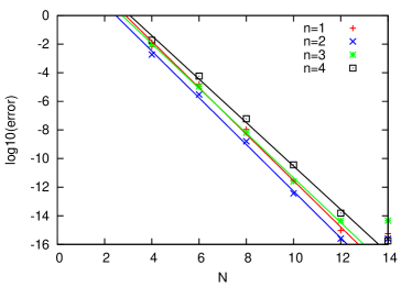
(i)	(ii)

Figure 2: The relative errors of the proposed method applied to the f.p. integrals (i) and (ii) in (10).

Table 1: The decay rates of the errors of the proposed method allied to the the f.p. integrals (i) and (ii) in (10).

$n$	1	2	3	4
integral (1)	$\mathrm{O}(0.024^{N})$	$\mathrm{O}(0.023^{N})$	$\mathrm{O}(0.027^{N})$	$\mathrm{O}(0.030^{N})$
integral (2)	$\mathrm{O}(0.28^{N})$	$\mathrm{O}(0.32^{N})$	$\mathrm{O}(0.31^{N})$	$\mathrm{O}(0.33^{N})$

4 Summary

In this paper, we proposed a numerical method of computing Hadamard finite part integrals with a non-integral power singularity on an endpoint. In the proposed method, we express the desired f.p. integral using a complex loop integral, and obtain the f.p. integral by evaluating the complex integral by the trapezoidal formula with equal mesh. Theoretical error estimate and some numerical examples showed the exponential convergence of the proposed method.

We can obtain similarly f.p. integrals on an infinite interval. This will be reported in a future paper.

References

• [1] M. Abramowitz and Irene A. Stegun (eds.). Handbook of Mathematical Functions with Formulas, Graphs and Mathematical Tables. Dover, New York, 1965.
• [2] B. Bialecki. A sinc-hunter quadrature rule for cauchy principal value integrals. Math. Comput., 55:665–681, 1990.
• [3] B. Bialecki. A sinc quadrature rule for hadamard finite-part integrals. Numer. Math., 57:263–269, 1990.
• [4] P. J. Davis and P. Rabinowitz. Methods of Numerical Integration, Second Ed. Academic Press, San Diego, 1984.
• [5] D. Elliot and D. F. Paget. Gauss type quadrature rules for cauchy principal value integrals. Math. Comput., 33:301–309, 1979.
• [6] R. Estrada and R. P. Kanwal. Regularization, pseudofunction, and hadamard finite part. J. Math. Anal. Appl., 141:195–207, 1989.
• [7] P. Henrici. Applied and Computational Complex Analysis, volume 2. John Wiley & Sons, New York, 1977.
• [8] H. Ogata. A numerical method for hadamard finite-part integrals with an integral power singularity at an endpoint, 2019. arXiv:1909.08872v1 [math.NA].
• [9] H. Ogata and H. Hirayama. Numerical integration based on hyperfunction theory. J. Comput. Appl. Math., 327:243–259, 2018.
• [10] H. Ogata, M. Sugihara, and M. Mori. De-type quadrature formulae for cauchy principal-value integrals and for hadamard finite-part itnegrals. In Proceedings of the Second ISAAC Congress, volume 1, pages 357–366, 2000.
• [11] D. F. Paget. The numerical evaluation of hadamard finite-part integrals. Numer. Math., 36:447–453, 1981.
• [12] H. Takahasi and M. Mori. Double exponential formulas for numerical integration. Publ. Res. Inst. Math. Sci., Kyoto Univ., 339:721–741, 1978.