Quantum memory and quantum correlations of Majorana qubits used for magnetometry

Abstract

We address how the non-local nature of the topological qubits, realized by Majorana modes and driven by an external magnetic field, can be used to control the non-Markovian dynamics of the system. It is also demonstrated that the non-local characteristic plays a key role in control and protection of quantum correlations between Majorana qubits. Moreover, we discuss how those non-local qubits help us to enhance quantum magnetometry.

Keywords: Topological qubits; quantum correlations, non-Markovianity, quantum magnetometry.

1 Introduction

Quantum correlations (e.g., entanglement [1] or discord [2, 3, 4]) are fundamental features of quantum mechanics and play significant roles in various potential applications, such as superdense coding, quantum teleportation, and quantum cryptography [5, 6, 7, 8]. Nevertheless, the quantum correlations are usually very fragile and broken by unwanted and unexpected interactions with an environment referred to as quantum noise. In fact, the decoherence effect generates correlations between the system and environment, leading to an irreversible loss of information from the system. Because there is no system which can be regarded as truly isolated, investigating the the dynamics of the quantum correlations (inside the system) under the action of noises and protecting these quantum resources against the effects of the environment are of great importance, and also major challenges for the realization of quantum computing devices [9, 10, 11].

Although the interaction with an environment causes the quantum system to dissipate energy and lose its coherence [12], this process needs not be monotonic and the system may recover temporarily some of the lost energy and/or information. This behaviour called non-Markovianity can be characterized and quantified in different ways (see [13, 14] for reviews). In this paper, we use the measures which are easy to compute and for which no external ancilla, attached to the open system of interest, is necessary to obtain the non-Markoianity.

The sudden change (death and birth) phenomenon (SCP) of quantum correlations and protecting them against the noise have been the themes of numerous works in the last few years. In the case of Markovian dynamics of quantum correlations, an interesting geometric interpretation of the sudden change behavior of quantum correlations, for the simple situation in which Bell-diagonal states are considered, was provided in Ref. [15], while the conditions for the correlations to stay constant, the so called freezing phenomena, were investigated in Ref. [16], focusing on the phase damping channel. Moreover, in Ref. [17], considering the case of Bell-diagonal states under the action of non-dissipative environments, the authors proved that all bona fide measures of quantum correlations virtually present the freezing effect under the same dynamical conditions. Besides, using the quantum discord as a measure for quantum correlations, the authors of [18] proved that a pure state never present the SCP and that the freezing phenomena is not a general property of all the Bell-diagonal states.

Because of memory effects, the non-Markovian channels may be more advantageous compared to Markovian ones. The case of two independent qubits subject to two zero-temperature non-Markovian reservoirs was investigated in Ref. [19], in which the dynamics of entanglement and quantum discord were compared with each other. The authors verified that while the quantum discord can only vanish at some specific time periods, the entanglement presents a sudden death such that it disappears for all times after the critical time-point. In Ref. [20] the authors discussed the similar problem, however they studied the case of a common reservoir, and again the SCP was observed. In addition, considering the class of Bell-diagonal states, the authors of Ref. [22] compared the non-Markovian dynamics of two geometric measures of quantum correlations with that of the quantum discord. Although all the three considered measures share a common sudden change point, one of the geometric measures does not present the freezing phenomenon. Besides, the dependence of the freezing effect on the choice of the correlation measure were also investigated in [23]. Moreover, in Ref. [24], the authors studied the non-Markovianity and information flow for qubits subject to local dephasing with an Ohmic class spectrum and demonstrated the existence of a temperature-dependent critical value of the Ohmicity parameter for the onset of non-Markovianity. They also unveiled a class of initial states for which the discord is forever frozen at a positive value. The investigation of the freezing phenomenon is very important because it guarantees that the quantum protocols, in which quantum correlations are used as resources, may be implemented such that they are unaffected by specific noisy conditions. Therefore, more analyses of the behaviour of quantum discord under different noisy quantum channels are necessary.

It has been seen that the topological quantum computation is a promising scheme for realizing a quantum computer with robust qubits [25]. In particular, there are new kinds of topologically ordered states, such as topological insulators and superconductors [26, 27, 28], which are easy to realize physically. Among different excitations for these these systems, the most interesting ones are the Majorana modes localized on topological defects, obeying the non-Abelian anyonic statistics [29, 30, 31]. The Kitaev’s 1D spineless p-wave superconductor chain model [32, 33, 34] is one of simplest scenario for realizing such Majorana modes. Each on-site fermion can be decomposed into two Majorana modes such that by appropriately tuning the model, the Majorana modes at the endpoints of Kitaev’s chain may be dangling without pairing with the other nearby Majorana modes, forming the usual fermions. Then, these two far separated endpoint Majorana modes can compose a topological qubit. The most important characteristic of the topological qubit is it is non-local, because the two Majorana modes are far separated. This non-locality causes the topological qubit to interact quite differently with the environment comparing it to the usual fermion. Motivated by this, we investigate how the non-local characteristic of the topological qubits can be used for controlling their dynamics and probing the environment.

Recent developments in the field of quantum metrology have shown that how quantum probes and quantum measurements allow us to achieve parameter estimation with precision beyond that achievable by any classical scheme [35, 36, 37, 38, 39, 40, 41, 42, 43]. Estimating the strength of a magnetic field [44, 45, 46, 47, 48] is a paradigmatic example in this respect, because it may be directly mapped to the problem of estimating the Larmor frequency for an atomic spin ensemble [49, 50, 51, 52, 53, 54, 55].

In this paper the non-Markovian dynamics of a topological qubit realized by two Majorana modes coupled to a fermionic Ohmic-like reservoir is discussed in detail. The fermionic environment is the helical Luttinger liquids realized as interacting edge states of two-dimensional topological insulators. Imposing a cutoff for the linear spectrum of the edge states, we illustrate the significant role of this cutoff in controlling the non-Markovian evolution of the system and determining when the Ohmic-like environment can exhibit non-Markovian behaviour. Moreover, we study the non-Markovian behaviour of two independent Majorana qubits, each locally interacting with its own reservoir and investigate the effects of the imposed cutoff, originated from the non-local nature of the topological qubits, on quantum correlations and specially protection of them against the noise. In addition, we use the topological qubits for the quantum magnetometry, i.e. quantum sensing of magnetic fields by quantum probes, and examine how their non-local characteristics help us to enhance the estimation.

This paper is organized as follows: In Secion 2, we present a brief review of the quantum correlation measures, quantum metrology and non-Markovianity measures. The model is introduced in Section 3. The non-Markovian behaviour of the single topological qubit is discussed in Sec. 4 and the study is extended to two-qubit scenario in Sec. 5 in which the different measures of quantum correlations are also addressed. Moreover, in Sec. 6 we explore the quantum magnetometry using entangled topological qubits. Finally in Section 7, the main results are summarized.

2 The Preliminaries

2.1 Quantum Correlation measures

2.1.1 Concurrence

In order to quantify the entanglement of the evolved state, we use concurrence [56, 57]. For $X$-type structure states defined as

$$\rho_{X}=\left(\begin{array}[]{cccc}\rho_{11}&0&0&\rho_{14}\\ 0&\rho_{22}&\rho_{23}&0\\ 0&\rho_{32}&\rho_{33}&0\\ \rho_{41}&0&0&\rho_{44}\\ \end{array}\right),$$ (1)

the concurrence may be obtained easily using a simple expression given by [58]

$$C(\rho)=2\text{max}\left\{0,\Lambda_{1}(\rho),\Lambda_{2}(\rho)\right\},$$ (2)

in which

$$\Lambda_{1}(\rho)=|\rho_{14}|-\sqrt{\rho_{22}\rho_{33}},\Lambda_{2}(\rho)=|\rho_{23}|-\sqrt{\rho_{11}\rho_{44}}.$$ (3)

where $\rho_{ij}$’s denote the elements of density matrix $\rho^{X}$. The concurrence is equal to zero for separable states and it equals to $1$ for maximally entangled states.

2.1.2 Quantum Discord

The usual quantum discord (QD), in terms of von Neumann entropy, is defined as difference between total correlations and classical correlations [59, 21]:

$$QD(\rho_{AB})=I(\rho_{AB})-\mathcal{C}(\rho_{AB}).$$ (4)

where

$$I(\rho_{AB})=S(\rho_{A})+S(\rho_{B})-S(\rho_{AB}).$$ (5)

$$\mathcal{C}(\rho_{AB})=S(\rho_{A})-\text{min}_{{\left\{\Pi^{B}_{k}\right\}}}S(\rho_{A}|B),$$ (6)

in which $I(\rho_{AB})$ denotes the quantum mutual information measuring the total correlations, including both classical and quantum, for a bipartite state $\rho_{AB}$. Besides, $S(\rho)=-\text{Tr}\left(\rho\text{log}_{2}\rho\right)$ represents the von Neumann entropy of a quantum state, and $\mathcal{C}(\rho_{AB})$ is a measure of classical correlations. The minimization is performed over all complete sets of projective measurements on subsystem $B$. Moreover, $S(\rho_{A|B})=\sum\limits_{k}p_{k}S(\rho^{k}_{A})$ represents the conditional entropy for subsystem A; $p_{k}=\text{Tr}\big{[}(I_{A}\otimes\Pi^{B}_{k})\rho_{AB}(I_{A}\otimes\Pi^{B}_{k})\big{]}$ and $\rho^{k}_{A}=\text{Tr}_{B}\big{[}(I_{A}\otimes\Pi^{B}_{k})\rho_{AB}(I_{A}\otimes\Pi^{B}_{k})\big{]}/p_{k}$ are respectively the probability and the state of subsystem A obtaining measurement outcome $k$.

2.1.3 Local quantum uncertainty

Although the quantum correlations measures are usually defined as a direct function of the density matrix $\rho$ itself, its other forms can also be advantageous. For example, the square root $\sqrt{\rho}$ in the well-known notion of the skew information has been used to study the local quantum uncertainty (LQU) which is an important measure of the quantum correlation. Assuming a bipartite quantum system prepared in quantum state $\rho=\rho_{AB}$, we suppose that $O^{\varLambda}\equiv O^{\varLambda}_{A}\otimes\mathcal{I}_{B}$ represents a local observable, in which $O^{\varLambda}_{A}$ denotes a Hermitian operator on subsystem $A$ with non-degenerate spectrum $\varLambda$. The LQU with respect to $A$ is defined as follows [60, 61]

$$\text{LQU}^{\varLambda}_{A}=\min_{O^{\varLambda}}I(\rho,O^{\varLambda}).$$ (7)

in which $I(\rho,O^{\varLambda})=-\dfrac{1}{2}\text{Tr}\{[\sqrt{\rho},O^{\varLambda}]^{2}\}$ represents the skew information. In addition, we should minimize over all local observables of $A$ with non-degenerate spectrum $\varLambda$.

2.1.4 Trace norm of discord

For a bipartite system described by the density matrix $\rho_{AB}$, the trace norm of discord (TND), a measure of the quantum correlation, is given by [61]

$$\mathcal{D}_{t}=\min_{\chi\in\mathcal{CQ}}||\rho_{AB}-\chi||,$$ (8)

where $||\rho_{AB}-\chi||=\text{Tr}\sqrt{(\rho_{AB}-\chi)^{\dagger}(\rho_{AB}-\chi)}$ represents the trace distance between $\rho_{AB}$ and $\chi\in\mathcal{CQ}$ where $\mathcal{CQ}=\{\rho_{\mathcal{CQ}}\}$ is the set of classical-quantum states that can be written as

$$\rho_{\mathcal{CQ}}=\sum\limits_{k}p_{k}\Pi^{A}_{k}\otimes\rho^{B}_{k},$$ (9)

a convex combination of the tensor products of the orthogonal projectors $\Pi^{A}_{k}$ for subsystem A and arbitrary density operators $\rho^{B}_{k}$ for subsystem B, with $\{p_{k}\}$ denoting any probability distribution. For a two-qubit X state $\rho_{AB}\equiv\rho$, the computation of the TND can be simplifed by [61, 62, 63]

$$\mathcal{D}_{t}=\frac{1}{2}\sqrt{\frac{\text{$\xi_{1}$}^{2}\text{$\xi_{max}$}-\text{$\xi_{2}$}^{2}\text{$\xi_{min}$}}{\text{$\xi_{1}$}^{2}-\text{$\xi_{2}$}^{2}+\text{$\xi_{max}$}-\text{$\xi_{min}$}}}$$ (10)

in which $\xi_{1,2}=2(|\rho_{23}|\pm|\rho_{14}|)$, $\xi_{3}=1-2(\rho_{22}+\rho_{33})$, $\xi_{max}=\max\{\xi^{2}_{3},\xi^{2}_{2}+x^{2}\}$, and $\xi_{min}=\min\{\xi^{2}_{1},\xi^{2}_{3}\}$ where $x=2(\rho_{11}+\rho_{22})-1$.

2.2 Non-Markovianity measures

We first remind some important definitions of the theory of open quantum systems. The time evolution of the density operator, describing the quantum state of an open system, is characterized by a time-dependent family of completely positive and trace preserving (CPTP) maps: $\mathcal{E}_{t}$, called the dynamical map: $\rho_{t}=\mathcal{E}_{t}(\rho_{0})$, in which $\rho_{0}$ denotes the density matrix of the open quantum system at initial time $t=0$. Supposing that the inverse of $\mathcal{E}_{t}$ exists for all times $t\geq 0$, and defining a two-parameter family of maps by means of

$$\mathcal{E}_{t,t_{p}}\equiv\mathcal{E}_{t}\circ\mathcal{E}_{t_{p}}^{-1},$$ (11)

one can write CPTP map $\mathcal{E}_{t}$ as a composite of the propagator $\mathcal{E}_{t,t_{p}}$ and $\mathcal{E}_{t_{p}}$:

$$\mathcal{E}_{t,0}=\mathcal{E}_{t,t_{p}}\circ\mathcal{E}_{t_{p},0}~{},~{}~{}~{}~{}~{}\forall~{}~{}0<t_{p}<t,$$ (12)

where $\mathcal{E}_{t,0}\equiv\mathcal{E}_{t}$. Although $\mathcal{E}_{t,0}$ and $\mathcal{E}_{t_{p},0}$ should be completely positive by construction, the map $\mathcal{E}_{t,t_{p}}$ need not be completely positive and not even positive because the inverse $\mathcal{E}_{t_{p}}^{-1}$ of a completely positive map $\mathcal{E}_{t_{p}}$ need not be positive. Composition (12), originating from the existence of the inverse for all positive times, allows us to introduce the notion of divisibility. The family of dynamical maps is said to be P-divisible when propagator $\mathcal{E}_{t,t_{p}}$ is positive as well as trace-preserving, and CP-divisible if $\mathcal{E}_{t,t_{p}}$ is CPTP for all $0<t_{p}<t$ [14]. In the latter scenario, one can interpret $\mathcal{E}_{t,t_{p}}$ as a legitimate quantum channel, mapping states at time $t_{p}$ into states at time $t$ [65].

In [66], Rivas, Huelga, and Plenio (RHP) suggested that the quantum evolution is called Markovian if and only if (iff) the corresponding dynamical map is CP-divisible. Another important characterization of non-Markovianity was presented by Breuer, Laine, and Piilo (BLP) who proposed that a non-Markovian process is characterized by a flow of information from the environment back into the open system [67, 68]. Assuming that $\mathcal{E}_{t}$ is invertible, one can show that under this condition the quantum process is Markovian iff $\mathcal{E}_{t}$ is P-divisible [69, 14].

The most important common features of all non-Markovianity measures presented in the following subsections is that they are founded on the nonmonotonic time evolution of certain quantities when the divisibility property is violated. Nevertheless, the inverse is not necessarily true; i.e., there may be nondivisible maps consistent with monotonic time evolution.

2.2.1 Breuer, Laine, Piilo (BLP) measure

The trace norm defined by $\parallel\rho\parallel=\text{Tr}\sqrt{\rho^{\dagger}\rho}=\sum\limits_{k}\sqrt{a_{k}}$, in which $a_{k}$’s denote the eigenvalues of $\rho^{\dagger}\rho$, yields a significant measure for the distance between two states $\rho^{1}$ and $\rho^{2}$ called trace distance [59] $D(\rho^{1},\rho^{2})=\frac{1}{2}\parallel\rho^{1}-\rho^{2}\parallel$. It may be proven that the trace distance $D(\rho^{1},\rho^{2})$ can be interpreted as the distinguishability between states $\rho^{1}$ and $\rho^{2}$. Besides, the trace distance is contractive for any CPTP map $\mathcal{E}$ [14], i.e., $D\big{(}\mathcal{E}(\rho^{1}),\mathcal{E}(\rho^{2})\big{)}\leq D(\rho^{1},\rho^{2})$, for any two quantum states $\rho^{1,2}$. Because any dynamical map $\mathcal{E}_{t}$ describing the dynamics of an open quantum system is necessarily CPTP, the trace distance between the time-evolved quantum states can never be larger than the trace distance between the initial states. Therefore, the dynamics decreases the distinguishability of the quantum states in comparison with the initial preparation. It should be noted that, this fact does not declare that $D\big{(}\rho^{1}(t),\rho^{2}(t)\big{)}$ where $\rho^{1,2}(t)\equiv\mathcal{E}_{t}(\rho^{1,2}(0))$ is a monotonically decreasing function with respect to time [70].

According to BLP definition [68, 67], for a divisible process, distinguishability of two initial quantum states $\rho^{1,2}$ diminishes continuously over time. Hence, a quantum evolution, mathematically defined by a quantum dynamical map $\mathcal{E}_{t}$, is called Markovian when, for all pairs of initial quantum states $\rho^{1}(0)$ and $\rho^{2}(0)$, trace distance $D\big{(}\rho^{1}(t),\rho^{2}(t)\big{)}$ decreases monotonically at all instants. Hence, quantum Markovian dynamics implies a continuous loss of information from the open system to the environment. On the other hand, a non-Markovian evolution is defined as a process in which, for certain time intervals,

$$\sigma(t,\rho^{1,2}(0))\equiv\dfrac{d}{dt}D\big{(}\rho^{1}(t),\rho^{2}(t)\big{)}>0,$$ (13)

i.e., the information flows back into the system temporarily, originating from appearance of quantum memory effects.

Following this, the measure of non-Markovianity $\mathcal{N}_{BLP}$ can be defined as [68]

$$\mathcal{N}_{BLP}(\mathcal{E}_{t})=\max_{\rho^{1,2}(0)}\int\limits_{\sigma>0}dt\sigma(t,\rho^{1,2}(0)).$$ (14)

where the maximization is performed over all the possible pairs of initial quantum states and the integration is calculated over all time intervals in which $\sigma$ is positive. It has been proved that [71, 69], for any non-Markovian quantum evolution of a single qubit, the maximum is achieved for a pair of pure orthogonal initial states corresponding to antipodal points on the Bloch sphere surface. Nevertheless, some challenges may be presented when one wishes to consider higher-dimensional systems of qubits [72, 73, 74]. Moreover, although the non-Markovian evolution defined in this way are always nondivisible, the converse is not necessarily true [75, 76].

2.2.2 Lorenzo, Plastina, Paternostro (LPP) measure

Another important proposed method to witness non-Markovianity was suggested by Lorenzo et al in [77]. First, these authors expand $\rho$, quantum state of a N-level open system, in the basis $\{G_{j}\}^{N^{2}-1}_{j=0}$, in which the identity $G_{0}=I/\sqrt{N}$ and $\{G_{j}\}^{N^{2}-1}_{j=1}$ are the Hermitian generators of SU(N) algebra [78],

$$\rho(t)=\mathcal{E}_{t}(\rho(0))=\sum\limits_{\alpha=0}^{N^{2}-1}\text{Tr}[\rho(t)G_{\alpha}]G_{\alpha}=\frac{I}{N}+\sum\limits_{\alpha=1}^{N^{2}-1}\text{Tr}[\rho(t)G_{\alpha}]G_{\alpha}=\sum\limits_{\alpha=0}^{N^{2}-1}r_{\alpha}G_{\alpha},$$ (15)

with $\vec{r}^{~{}t}=(1/\sqrt{N},\vec{\textbf{r}})^{~{}t}$ in which $\vec{\textbf{r}}=(r_{1},...,r_{N^{2}-1})^{~{}t}$ is called the generalized Bloch vector, and where $r_{\alpha}\equiv\text{Tr}[\rho(t)G_{\alpha}]$. Then, it can be proven that the action of the dynamical map can be considered as an affine transformation of the initial state Bloch vector $\vec{\textbf{r}_{0}}$ [13],

$$\rho(t)=\mathcal{E}_{t}(\rho(0))\longleftrightarrow\vec{\textbf{r}}=\textbf{M}(t)\vec{\textbf{r}_{0}}+\vec{\textbf{c}}(t)$$ (16)

where $[\textbf{M}(t)]_{ij}=\text{Tr}[G_{i}\mathcal{E}_{t}(G_{j})]$ and $[\vec{\textbf{c}}(t)]_{i}=\text{Tr}[G_{i}\mathcal{E}_{t}(I)]/N$ for $i,j>0$. As discussed in [77], the time-variation of $|\text{det}[\textbf{M}(t)]|$ describes the change in volume of the set of states accessible through the evolution of the reduced state. Because the Markovian evolution reduces (or leaves invariant) the volume of accessible states, the following measure has been proposed [77] to quantify the non-Markovianity of a quantum evolution,

$$\mathcal{N}_{LPP}(\mathcal{E}_{t})=\int\limits_{\partial_{t}|\text{det}[\textbf{M}(t)]|>0}\text{d}t\dfrac{\text{d}}{\text{d}t}|\text{det}[\textbf{M}(t)]|.$$ (17)

2.2.3 Chanda and Bhattacharya (CB) measure

Quantum coherence originating from the superposition principle plays a key role in quantum mechanics such that it is a significant resource in quantum information theory. For a quantum state with the density matrix $\rho$, the $l_{1}$-norm measure of quantum coherence [64] quantifying the coherence through the off diagonal elements of the density matrix in the reference basis, is given by

$$\mathcal{C}_{l_{1}}\left(\rho\right)=\sum_{i,j\atop i\neq j}|\rho_{ij}|.$$ (18)

In the basis $\{|i\rangle\}_{i=1,...,d}$, all of the diagonal density matrices, i.e., $\varrho=\sum\limits_{i=1}^{d}c_{i}|i\rangle\langle i|$ are called incoherent states, while the states of the form $|\Psi_{d}\rangle=\frac{1}{\sqrt{d}}\sum\limits_{j=1}^{d}\text{e}^{i\phi_{j}}|j\rangle,~{}~{}0<\phi_{j}<2\pi,$ are recognized as maximally coherent states.

For incoherent dynamics described by the incoherent operation $\Lambda_{t}$, a CPTP map which always maps any incoherent state to another incoherent one, the authors of [79] proposed the following non-Markovianity measure based on $l_{1}$-norm measure of quantum coherence $\dfrac{dC_{l_{1}}(\rho(t))}{dt}$

$$\mathcal{N}_{CB}(\Lambda_{t})=\max_{\rho(0)\in\Im^{c}}\int\limits_{{}_{\dfrac{dC_{l_{1}}(\rho(t))}{dt}>0}}~{}\dfrac{dC_{l_{1}}(\rho(t))}{dt}dt,$$ (19)

in which maximization should be performed over all the initial coherent states $\rho(0)$ creating the set $\Im^{c}$. Because in the case of large systems (i.e., large d), the above maximization procedure may be complex to compute, a nonoptimized version of the measure can be used in those cases,

$$\mathcal{N}^{l}_{CB}(\Lambda_{t})=\max_{\rho(0)\in\{|\Psi_{d}\rangle\langle\Psi_{d}|\}}\int\limits_{{}_{\dfrac{dC_{l_{1}}(\rho(t))}{dt}>0}}~{}\dfrac{dC_{l_{1}}(\rho(t))}{dt}dt,$$ (20)

Generally, the maximization over all possible initial states involved in quantifying non-Markovianity is necessarily demanding. Nevertheless, starting with any chosen set of initial states, one can always obtain lower bounds to the measure of non-Markovianity, and hence achieve a qualitative assessment of the non-Markovian character of the evolution [80].

3 The Model

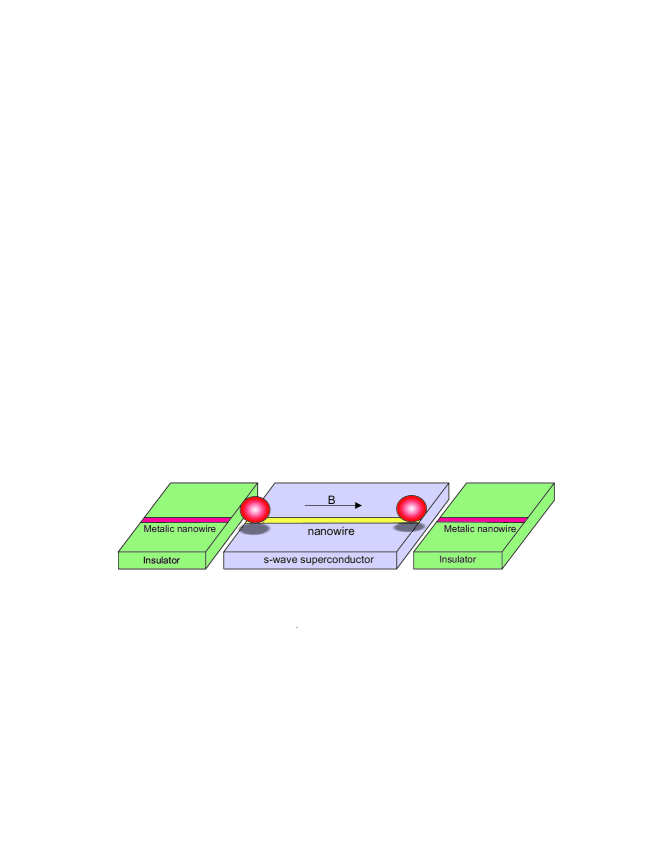
Figure 1: Schematic diagram for the Majorana qubit coupled to the fermionic environment.

We consider a topological qubit realized by Majorana modes, generated at the endpoints of some nanowire with strong spin-orbit interaction, driven by an external magnetic field B along the wire axis direction, and placed on top of an s-wave superconductor (see Fig. 1). Each of the Majorana modes is coupled to the metallic nanowire via a tunnel junction such that the tunneling strength is controllable via an external gate voltage.

The total Hamiltonian is given by

$$H=H_{S}+H_{E}+V$$ (21)

where $H_{s}$ is the Hamiltonian of the topological qubit and $V$ denotes the system-environment interaction Hamiltonian. Moreover, the environment Hamiltonian is represented by $H_{E}$ whose elementary constituents can be thought of as electrons. The decoherence affecting the topological qubit may be modelled as a fermionic Ohmic-like environment characterize by spectral density $\rho_{spec}\propto\omega^{Q}$ with $Q\geq 0$. The environment is called Ohmic for $Q=1$, super-Ohmic for $Q>1$ and sub-Ohmic for $Q<1$. This is realized by placing a metallic nanowire close to the Majorana endpoint. More specifically the fermionic environment chosen in this paper is the helical Luttinger liquids realized as interacting edge states of two-dimensional topological insulators [81]. Because these Majorana modes used for the qubits are zero-energy modes, we have $H_{S}=0$. Besides, the interaction Hamiltonian $V$ is constructed by the electrons creation (annihilation) operators, and Majorana modes $\gamma_{1}$ as well as $\gamma_{2}$ having the properties:

$$\gamma^{\dagger}_{a}=\gamma_{a},~{}~{}~{}\{\gamma_{a},\gamma_{b}\}=2\delta_{ab},$$ (22)

where $a,b=1,2$. The following representation can be chosen for $\gamma_{1,2}$:

$$\gamma_{1}=\sigma_{1},~{}~{}~{}\gamma_{2}=\sigma_{2},~{}~{}~{}\text{i}\gamma_{1}\gamma_{2}=\sigma_{3},$$ (23)

in which $\sigma_{j}$’s denote the Pauli matrices. Before turning on the interaction $V$, the two Majorana modes form a topological (non-local) qubit with states $|0\rangle$ and $|1\rangle$ according to the following relations:

$$\frac{1}{2}(\gamma_{1}-\text{i}\gamma_{2})|0\rangle=|1\rangle,~{}~{}~{}~{}~{}\frac{1}{2}(\gamma_{1}+\text{i}\gamma_{2})|1\rangle=|0\rangle.$$ (24)

Suppose that $\varrho^{T}$, describing the state of the total system, is uncorrelated initially: $\varrho^{T}(0)=\varrho(0)\otimes\varrho_{E}$, where $\rho_{S}(0)$ and $\rho_{E}$ denote the initial density matrices of the topological qubit and its environment, respectively. Assuming that the initial state of the Majorana qubit is given by

$$\varrho(0)=\left(\begin{array}[]{cc}\varrho_{11}(0)&\varrho_{12}(0)\\ \varrho_{21}(0)&\varrho_{22}(0)\\ \end{array}\right),$$ (25)

we can find that the reduced density matrix at time $t$ is obtained as follows (for details, see [82]):

$$\varrho(t)=\frac{1}{2}\left(\begin{array}[]{cc}1+(2\varrho_{11}(0)-1)\alpha^{2}(t)&2\varrho_{12}(0)\alpha(t)\\ 2\varrho_{21}(0)\alpha(t)&1+(2\varrho_{22}(0)-1)\alpha^{2}(t)\\ \end{array}\right),$$ (26)

where

$$\alpha=\text{e}^{-2B^{2}|\beta|I_{Q}},~{}~{}~{}~{}~{}\beta\equiv\dfrac{-4\pi}{\Gamma(Q+1)}(\dfrac{1}{\varGamma_{0}})^{Q+1}$$ (27)

in which $\varGamma_{0}$ represents the high-frequency cutoff for the linear spectrum of the edge state and $\Gamma(z)$ denotes the Gamma function. Moreover,

$$I_{Q}=\left\{\begin{array}[]{rl}2\varGamma_{0}^{Q-1}\Gamma(\frac{Q-1}{2})\bigg{[}1-\,_{1}F_{1}\big{(}\frac{Q-1}{2};\frac{1}{2};-\frac{t^{2}\varGamma^{2}_{0}}{4}\big{)}\bigg{]}&~{}~{}~{}~{}~{}~{}~{}~{}\text{for}~{}Q\neq 1,\\ \frac{1}{2}t^{2}\varGamma^{2}_{0}\,{}_{2}F_{2}\bigg{(}\{1,1\};\{3/2,2\};-\frac{t^{2}\varGamma^{2}_{0}}{4}\bigg{)}&~{}~{}~{}~{}~{}~{}~{}~{}\text{for}~{}Q=1,\end{array}\right.$$ (28)

where $\,{}_{p}F_{q}$ denotes the generalized hypergeometric function and $\varGamma(z)$ represents the Gamma function.

4 Non-Markovian dynamics of the one-qubit system

In this section, the non-Markovian evolution of the qubit described by density matrix (26) is investigated.

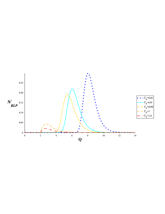
Figure 2: Non-Markovianity $\mathcal{N}_{BLP}$ versus $Q$ for different values of $\varGamma_{0}$.

In order to compute non-Markovianity $\mathcal{N}_{BLP}$, one has to find a specific pair of optimal initial states maximizing the time derivative of the trace distance. As pointed out in Sec. 2.2.1, for any non-Markovian evolution of a qubit, the maximal backflow of information occurs for a pair of pure orthogonal initial states corresponding to antipodal points on the surface of the Bloch sphere. Using numerical simulation, we can show that for our model the optimal initial states are $\{|0\rangle,|1\rangle\}$. The trace distance between these two states is $D\big{(}\rho^{1}(t),\rho^{2}(t)\big{)}=\alpha^{2}(t)$, leading to $\mathcal{N}_{BLP}=\int\text{d}t\big{(}\dfrac{\text{d}\alpha^{2}(t)}{\text{d}t}\big{)}$ where the integration is performed over region $\dfrac{\text{d}\alpha^{2}(t)}{\text{d}t}>0$. The results are illustrated in Fig. 2: as apparent from the plot, there is a critical value of $Q$ at which the non-Markovianity appears and an optimal value of $Q$ for which the backflow of information from the environment to the system is maximized. Moreover, we see that an increase in cutoff $\varGamma_{0}$ reduces the optimal value of $Q$ at which $\mathcal{N}_{BLP}$ is maximized and it also decreases the critical value of $Q$ at which the non-Markovianity rises. The existence of a cutoff-dependent critical value of the Ohmicity parameter, ruling the Markovian to non-Markovian transition, is one of the main results of this paper. Nevertheless, it is found that there exists a threshold value $Q_{th}=2$ such that when $Q<2$ the non-Markovianity completely vanishes, although increasing cutoff $\varGamma_{0}$. By changing the $Q$ parameter, we go from sub-Ohmic reservoirs ($Q<1$) to Ohmic ($Q=1$) and super-Ohmic ($Q>1$) reservoirs, respectively. Therefore, when the fermionic environment is Ohmic or sub-Ohmic the evolution of the Majorana qubit does not exhibit non-Markovian effects. On the other hand, as seen from the figure, the dynamics can be strongly non-Markovian for small values of the cutoff, while an increase in cutoff suppresses the non-Markovianity and memory effects.

Wee introduce parameter $\kappa\equiv\big{(}K+\dfrac{1}{K}\big{)}/4$, where $K$ characterizes the Luttinger liquid, e.g., $\kappa=1/2$ for Fermi liquid. A rough estimation of the Luttinger parameter $K$ is given by $K^{2}\sim\big{(}1+\dfrac{U}{2\epsilon_{F}}\big{)}$ in which $\epsilon_{F}$ represents the Fermi energy and $U\sim\dfrac{e^{2}}{\epsilon a_{0}}$, where $\epsilon$ and $a_{0}$, respectively, are the dielectric constant and the lattice length, denotes the characteristic Coulomb energy of the wire [83]. It is known that the Coulomb interaction of the metallic wire can be tuned by choosing a different insulating substrate or gating. Therefore, the value of $\kappa$ may be tuned by varying the effective repulsive/attractive short range interactions in the wire. Recalling that $Q=2\kappa-1$, we should note that parameter $\kappa$ characterizes the interaction strengths of the Luttinger/Fermi liquid. The larger $\kappa$, the stronger the correlation/interaction exhibited by the Luttinger liquid nanowire. Combining these points with the results obtained from Fig. 2, we find that the non-Markovianity vanishes when the environments are so weakly ($\kappa<3/2$) or very strongly correlated ($\kappa\rightarrow\infty$). Moreover, although it has been assumed that the coupling between the Majorana modes and the environment to be weak such that the Gaussian approximation holds well [82], the non-Markovianity, controllable by the cutoff, may occurs with correlated environments.

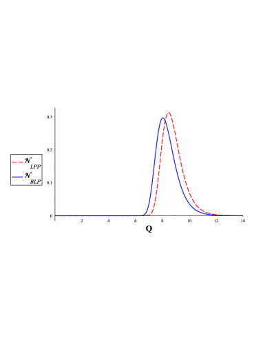
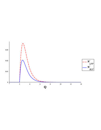
Figure 3: The BLP and LPP measures of non-Markovianity versus Q for (a) $\varGamma_{0}=0.01$ and (b) $\varGamma_{0}=1.6$.

Now we compare BLP and LPP measures in the process of detecting the non-Markovian dynamics of the topological qubit. Using the approach introduced in Sec. 2.2.2, one can show that $\textbf{M}(t)=\text{diag}(\alpha(t),\alpha(t),\alpha^{2}(t))$, leading to $\text{det}[\textbf{M}(t)]=\alpha^{4}(t)$ and consequently $\mathcal{N}_{LPP}=\int\text{d}t\big{(}\dfrac{\text{d}\alpha^{4}(t)}{\text{d}t}\big{)}$ in which the integration should be performed over region $\dfrac{\text{d}\alpha^{4}(t)}{\text{d}t}>0$. Plotting $\mathcal{N}_{LPP}$, we again obtain exactly the similar results extracted from Fig. 2. Nevertheless, as shown in Fig. 3 , the LPP measure is not as efficient as BLP measure in detecting the non-Markovianity when the cutoff is small. However, for larger values of the cutoff, the two measures qualitatively exhibit the same behaviour, i.e., approximately the LPP is as sensitivity as BLP measure to detect non-Markovianity (see Fig. 3).

.

5 Quantum correlations and non-Markovian dynamics of the two-qubit system

In order to study the dynamics of quantum correlations for Majorana qubits, we need the expression of the two-qubit density matrix. As known for the case that the subsystems interact independently with their environments, the complete dynamics of the two-qubit system can be computed by knowing the reduced density matrices of each qubit [84, 85] (see Appendix A). We focus our analysis on the initial entangled state $\rho_{0}=|\psi_{0}\rangle\langle\psi_{0}|$ where

$$|\psi_{0}\rangle=\cos(\vartheta/2)|00\rangle+\sin(\vartheta/2)|11\rangle.$$ (29)

Therefore, the nonzero matrix elements of the evolved density matrix are given by

$$\rho_{1,1}(t)=\dfrac{1}{4}\,{\alpha}^{4}+\dfrac{1}{2}\,\cos\left(\vartheta\right){\alpha}^{2}+\dfrac{1}{4},~{}~{}\rho_{2,2}(t)=\rho_{3,3}(t)=-\dfrac{1}{4}\,{\alpha}^{4}+\dfrac{1}{4},$$

$$\rho_{4,4}(t)=1-\bigg{(}\rho_{1,1}(t)+\rho_{2,2}(t)+\rho_{3,3}(t)\bigg{)};~{}~{}\rho_{1,4}(t)=\rho_{4,1}(t)=\frac{1}{2}\,{\alpha}^{2}\sin\left(\vartheta\right).$$ (30)

Computing (20) for the above dynamics leads to a lower bound on the degree of non-Markovianity of the two-qubit evolution. Because $\mathcal{C}_{l_{1}}=\alpha^{2}(t)\text{sin}\vartheta$, it is found that this lower bound (with $\vartheta=\pi/2$) and the BLP measure for the one-qubit dynamics coincide exactly. Now this phenomenon is discussed using the quantum correlations between the two qubits and their efficiency in detecting the non-Markovian behaviour of the composite system is investigated. According to our computed results, the bipartite entanglement, as quantified by concurrence, is given by

$$C(\rho(t))=2\,\text{max}\left(0,\dfrac{{\alpha}^{2}}{2}\sin\left(\vartheta\right)-\dfrac{\left|{\alpha}^{4}-1\right|}{4}\right).$$ (31)

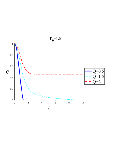
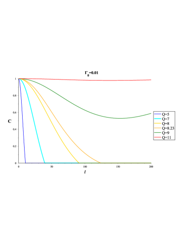
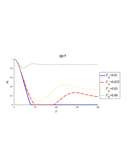
Figure 4: The time variation of the concurrence for (a), (b) different values of Ohmicity parameter $Q$ in Markovian and non-Markovian regimes. (c) The same quantity for different values of cutoff $\varGamma_{0}$.

Figure 4 shows that the entanglement may decrease abruptly and non-smoothly to zero in a finite time due to the influence of quantum noise. This non-smooth finite-time decay is called entanglement sudden death (ESD) which may occur in both Markovian and non-Markovian dynamics, as seen in Fig. 4. In Markovian regime, if the ESD occurs the entanglement cannot be restored over time, while in non-Markovian regime it is sometimes possible to recover the entanglement, however this recovery is not guaranteed. In fact, in non-Markovian regime the ESD can occur only for small values of $\varGamma_{0}$. The ESD may exhibit robustness, even when the $Q=Q_{\text{opt}}$ at which the non-Markovianity is maximized. However, increasing $Q$ $(Q>Q_{\text{opt}})$ can remove the sudden death and protect the entanglement over time in both markovian and non-Markovian dynamics (see Figs. 4 and 4). This revival phenomenon is induced by the memory effects of the reservoirs, which allows the two-qubit to reappear their entanglement after a dark period of time, during which the concurrence is zero. Another important feature illustrated in Fig. 4 is the high level of quantum control realized by imposing a cutoff $\varGamma_{0}$. The plot shows that increasing the cutoff, we can remove the entanglement ESD and also protect the initial maximal entanglement over time. Moreover, we observe the suppressive role of the cutoff on non-Markovian dynamics, leading to reduction of the oscillations amplitude in entanglement dynamics.

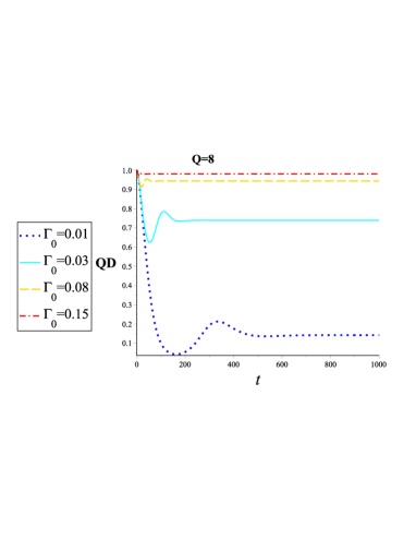
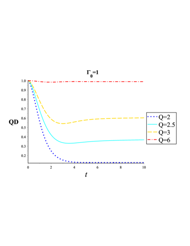
Figure 5: (a) The QD as a function of time for different values of cutoff $\varGamma_{0}$. (b) The same quantity for different values of Ohmicity parameter $Q$.

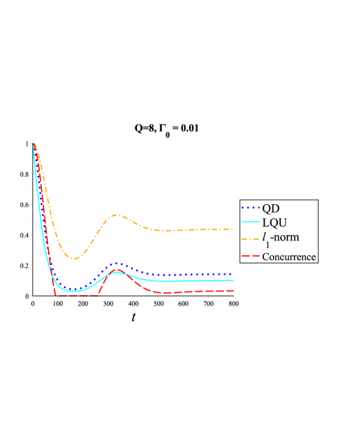
Figure 6: Comparing the dynamics of different quantum correlation measures with the coherence.

The analytical expression for the QD associated with the density matrix, whose elements are given in Eq. (5), is presented in Appendix B. The dynamics of the QD is similar to one observed for the concurrence, except that the QD exhibits no sudden death (see Fig. 5). Another important characteristic of this measure of quantum correlations in our model is that the time variation of the QD may be stopped and the QD can remain approximately constant over time after a while, a phenomenon known as freezing of QD. In particular, Fig. (5) clearly shows that increasing $\varGamma_{0}$ or $Q$ such that the non-Markovianity is suppressed, we can approximately obtain the time-invariant discord. This phenomenon also may occur for $Q<2$ for which the dynamics is always Markovian provided that a large cutoff is imposed. It is also interesting to compare the behaviour of different quantum correlation measures and coherence. We find that for initial state (29), the TND and LQU, respectively, are given by

$$TND=\frac{1}{2}\mathcal{C}_{l_{1}}=\frac{1}{2}\alpha^{2}(t)\text{sin}\vartheta,~{}~{}~{}LQU_{\vartheta=\frac{\pi}{2}}=1-\sqrt{1-\alpha^{4}}.$$ (32)

A more general expression for the LQU is presented in Appendix B. Figure 6 illustrates the dynamics of quantum correlations, allowing us to compare them with the quantum coherence and hence analyze their efficiency in detecting the non-Markovianity. We see that the quantum entanglement between the qubits is not a reliable witness to detect the non-Markovianity because there exists some period of time at which the quantum coherence increases while the entanglement has vanished. However, the QD or discord-like measures including LQU, and TND exhibit qualitatively the same dynamics as coherence. Therefore the revival of each of these quantum correlation measures can be attributed to the memory effects of the reservoirs. Moreover, we can conclude that the coherence and quantum-discord like measures all freeze under the same dynamical conditions, albeit this phenomenon occurs after a while in the case of Markovian dynamics.

We also observe that under the dynamics considered here, discord-like measures are more robust than entanglement, and hence they are immune to the sudden death. This important phenomenon points to the fact that the absence of entanglement does not necessarily lead to the absence of quantum correlations. In addition, it suggests that quantum computers based on the quantum correlations, different from those based on entanglement, are more robust against the external perturbations and hence encourages us to try to implement an efficient quantum computer. Moreover, it mentions why some quantum algorithms can work well in the absence of entanglement. In fact, the QD must be larger than zero in the implementation of those algorithms in the situations that the entanglement is missed or destroyed by decoherence.

An important question which might be asked is why the ESD experienced by the concurrence, is not exhibited by the discord-like measures. This phenomenon can be interpreted by analyzing the behavior of the coherence. As discussed by some researchers, the QD is equal to the quantum coherence in a set of mutually unbiased bases for Bell-diagonal states [86]. Accordingly, the sudden birth and sudden death of the QD can be regarded as sudden birth and sudden death of quantum coherence in an optimal basis. In our work, because the quantum coherence exhibits no sudden birth or death, the QD also shows the similar behavior. It should be noted that both the quantum coherence and QD are parts of total correlation, i.e., quantum mutual information, and coherence is a more basic quantum resource for quantum information tasks [86]. The difference between the QD and entanglement can also be understood from a geometrical viewpoint: sudden death of entanglement happens when the evolving density matrix crosses the boundary into the set of unentangled (separable) states, where it can remain permanently, or for a finite period of time. However, the QD vanishes only on a lower-dimensional manifold within the set of density matrices, and hence we would expect the QD to vanish completely at most only at particular instants of time, when the evolving density matrix crosses this manifold. More specifically, K. Modi et al., [87] proposed such geometrical interpretation of correlations which considers the concurrence as the distance in Hilbert space between the quantum state of the system and the nearest separable state and QD as the distance to the nearest classical pure state. From that perspective one may say that for most of the states in the family the separable states are close, while at the same time the classical pure states are far in Hilbert space.

6 Quantum magnetometry

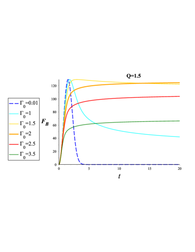
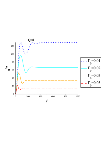
Figure 7: The time variation of the QFI associated with the magnetometry for different values of cutoff $\varGamma_{0}$ in (a) Markovian and (b) non-Markovian regimes.

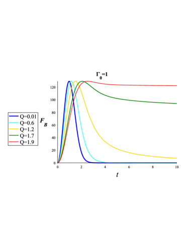
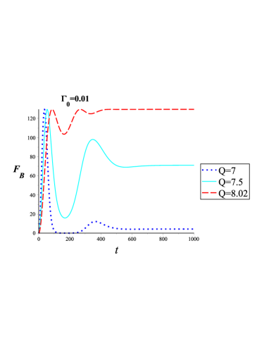
Figure 8: The time variation of the QFI associated with the magnetometry for different values of Ohmicity parameter $Q$ in (a) Markovian and (b) non-Markovian regimes.

The best possible precision of the parameter to be estimated is given by the Cramér-Rao bound: Let us suppose that one performs $N$ independent measurements in order to achieve an unbiased estimator $\hat{\eta}$ [88, 89] for parameter $\eta$ (such that $\text{Tr}[\rho_{\eta}\hat{\eta}]=\eta$). It can be shown that the variance of the estimator is lower bounded by $\langle(\hat{\eta}-\langle\hat{\eta}\rangle)^{2}\rangle\geq\dfrac{1}{NF_{\eta}}$ [90] where $F_{\eta}$ denotes the quantum Fisher information (QFI) [91, 90, 92, 93, 94, 95, 96], given by

$$F_{\eta}=\sum_{i,j}\frac{2}{\omega_{i}+\omega_{j}}|\langle\phi_{i}|\frac{\partial\rho_{\eta}}{\partial\eta}|\phi_{j}\rangle|^{2},$$ (33)

for the mixed state with spectral decomposition $\rho_{\eta}=\sum_{i}\omega_{i}|\phi_{i}\rangle\langle\phi_{i}|$.

We consider a scheme in which the two-qubit system, prepared initially in maximally entangled state (29), is used to sense the intensity of the external magnetic field driving the topological qubits. The QFI associated with the magnetometry is given by:

$$F_{B}=128\,{\frac{{\alpha}^{2}{B}^{2}|\beta|^{2}{I^{2}_{Q}}{~{}\text{e}^{-4\,{B}^{2}\left|\beta\right|I_{Q}}}}{1-{\alpha}^{4}}}.$$ (34)

On one hand, the information about the intensity of the magnetic field, encoded into the quantum state of the system, is able to flow into the environment. On the other hand, the system continously encodes the information because of the interaction with the magnetic field. In Markovian regime, as illustrated in Fig. 7, these two mechanisms compete with each other and in non-Markovian regime the quantum memory is added to this competition (see Fig. 7 ). In both Markovian and non-Markovian regimes, the QFI initially increases since the information is encoded into the quantum state because of the interaction with the magnetic field. Then the decoherence effect dominates the dynamics of the topological qubits leading to loss of encoded information, although in non-Markovian evolution the quantum memory may stop this process and help the interaction mechanism to temporarily increase the QFI. Moreover, the important role of the cutoff in controlling the dynamics and extracting the information from the Majorana system is clear from Fig. 7. It shows that in Markovian evolution, with increasing cutoff $\varGamma_{0}$, the QFI degradation can be frustrated. In fact, after a while, the QFI can remain approximately constant over time, a phenomenon known as QFI trapping. Although freezing of the QFI would be satisfactory and lets us protect the encoded information, the QFI may be suppressed by imposing larger values of the cutoff. In non-Markovian regime the QFI tapping always appears after a while and the QFI suppression also occurs when the cutoff increases.

Now we focus on effects of the Ohmicity parameter on the dynamics of the QFI. Figure 8 exhibits an important and interesting consequence of an increase in parameter $Q$ in Markovian regime ($Q<2$), leading to retardation of the QFI loss during the time evolution and therefore enhance the estimation of the parameter at a later time. Moreover, when the Ohmicity parameter varies from 0 to 2, the optimal value of estimation is not affected by this variation. Nevertheless, varying $Q$ from $0$ to $2$, we see that the QFI reaches its maximum value at a later time-point, and hence the instant at which the optimal estimation occurs is achieved later. On the other hand, in non-Markovian regime we find that when the Ohmicity parameter approaches the value $Q_{\text{opt}}$ at which the non-Markovianity is maximized, the QFI can be frozen at its optimal value (compare Figs. 8 and 2). Overall, the best estimation is obtained when $Q\approx Q_{\text{opt}}$ and when $Q\gg Q_{\text{opt}}$, the QFI approaches zero.

7 Summary and conclusions

To summarize, we investigated the quantum correlations and non-Markovian dynamics of Majorana qubits coupled to Ohmic-like fermionic environments and used for magnetometry. The fermionic environment is the helical Luttinger liquids realized as interacting edge states of two-dimensional topological insulators. The influence functional $\alpha$, appeared in the evolved density matrix of the topological qubit (see Eq. (26)), leads to imposition of a cutoff for the linear spectrum of the edge states, playing an important role in the dynamic of the system. In fact, this influence functional is the exclusive characteristic of topological qubits [82], in contrast with the one for non-topological qubits. Hence, the introduced cutoff, which can be applied as a control parameter for non-Markovian evolution of the system, results from the non-local nature of the topological qubits and the peculiar algebra of the Majorana modes. We discovered the existence of a cutoff-dependent critical value of the Ohmicity parameter for the Markovian to non-Markovian crossover. It was illustrated that the memory effects leading to information backflow and recoherence appear only if the reservoir spectrum is super-Ohmic with $Q>2$, however this critical value can be controlled by the cutoff. These results are consistent with ones obtained in [24] in which the authors discussed the existence of a temperature-dependent critical value of the Ohmicity parameter for the onset of non-Markovianity in local qubits experiencing dephasing with an Ohmic class spectrum. However, our results are different from ones presented in [82] in which the advent of non-Markovianity for super-Ohmic environment driving the topological qubit, has been claimed for $Q>1$ and the independence of presented results from the choice of the cutoff has been emphasized.

We also investigated the ESD, disruptive to quantum information processing due to the fast disappearance of entanglement. It was shown that the ESD may occur in both Markovian and non-Markovian dynamics. In Markovian regime, if the ESD occurs the entanglement cannot be restored over time. However, in non-Markovian regime we observed the counterintuitive entanglement rebirth after its sudden death or disappearance of the ESD by increasing the cutoff, demonstrating the high level of quantum control realized by imposing the cutoff. The entanglement sudden death or rebirth have been also implemented experimentally within linear optics set-up with photonic qubits [97, 98] and between atomic ensembles [99]. In Ref. [100], it has been shown that the ESD in a bipartite system independently coupled to two reservoirs is necessarily related to the entanglement sudden birth between the environments. In fact, the loss of entanglement is related to the birth of entanglement between the reservoirs and other partitions. The above study can easily be extended to investigate the entanglement dynamics starting from different initial conditions and to take into account finite temperature effects.

We then showed that the various quantum correlations and quantum coherence may be approximately frozen for all time by imposing a large cutoff and hence the time-invariant quantum resources may be realized with good approximation. The phenomenon of freezing of quantum discord has not remained as a purely theoretical construct. It has been several experiments demonstrating these peculiar effects with different physical systems such as optical experimental setup [101] and room temperature nuclear magnetic resonance setup [102].

Finally, we investigated the effects of the cutoff and Ohmicity parameter on the dynamics of the QFI. It was found that imposing large values of the cutoff is not satisfactory because of the QFI suppression. On the other hand, for different values of $Q$, we illustrated that the QFI associated with the magnetometry initially increases. In [103], it was proposed that a positive QFI flow at time t, i.e., $\dfrac{dF}{dt}>0$, implies that the QFI flows back into the system from the environment, generating a non-Markovian dynamics. However, in our estimation, the positivity of $\dfrac{dF_{B}}{dt}$ does not necessarily detect the non-Markovianity [104], because we have focused on estimating one of the environment parameters. In fact, when the probes interact with the environment, the information about the intensity of the magnetic field is encoded into the quantum state of the probes, and hence the QFI increases. According to theory of quantum metrology, an increase in the QFI indicates that the optimal precision of estimation is enhanced. However, simultaneously the interaction with the environment leads to flow of encoded information from the system to the environment. When this decoherence effect overcome the encoding process, its destructive influence appears and we see that the QFI monotonously decays with time, resulting in the quantum magnetometry becomes more inaccurate.

Appendix A Density matrix elements for two Majorana qubits independently interacting with the fermionic environments

In the standard basis $\{|00\rangle\equiv|1\rangle,|01\rangle\equiv|2\rangle,|10\rangle\equiv|3\rangle,|11\rangle\equiv|4\rangle\}$, using the approach introduced in [84] and considering (25), we find that the diagonal and non-diagonal elements of the density matrix for the two-qubit system, respectively, are given by:

$$\rho_{1,1}(t)=\frac{1}{4}\big{(}1+\alpha^{2}(t)\big{)}^{2}\rho_{1,1}(0)+\frac{1}{4}\big{(}1-\alpha^{2}(t)\big{)}^{2}\rho_{44}(0)+\frac{1}{4}\big{(}1-\alpha^{4}(t)\big{)}\big{[}\rho_{2,2}(0)+\rho_{3,3}(0)\big{]},$$

$$\rho_{2,2}(t)=\frac{1}{4}\big{(}1+\alpha^{2}(t)\big{)}^{2}\rho_{2,2}(0)+\frac{1}{4}\big{(}1-\alpha^{2}(t)\big{)}^{2}\rho_{3,3}(0)+\frac{1}{4}\big{(}1-\alpha^{4}(t)\big{)}\big{[}\rho_{1,1}(0)+\rho_{4,4}(0)\big{]},$$ (35)

$$\rho_{3,3}(t)=\frac{1}{4}\big{(}1+\alpha^{2}(t)\big{)}^{2}\rho_{3,3}(0)+\frac{1}{4}\big{(}1-\alpha^{2}(t)\big{)}^{2}\rho_{2,2}(0)+\frac{1}{4}\big{(}1-\alpha^{4}(t)\big{)}\big{[}\rho_{1,1}(0)+\rho_{4,4}(0)\big{]},$$

$$\rho_{4,4}(t)=\frac{1}{4}\big{(}1+\alpha^{2}(t)\big{)}^{2}\rho_{4,4}(0)+\frac{1}{4}\big{(}1-\alpha^{2}(t)\big{)}^{2}\rho_{1,1}(0)+\frac{1}{4}\big{(}1-\alpha^{4}(t)\big{)}\big{[}\rho_{2,2}(0)+\rho_{3,3}(0)\big{]},$$

and

$$\rho_{1,2}(t)=\frac{1}{2}\alpha(t)\big{(}1+\alpha^{2}(t)\big{)}\rho_{1,2}(0)+\frac{1}{2}\alpha(t)\big{(}1-\alpha^{2}(t)\big{)}\rho_{3,4}(0),$$

$$\rho_{1,3}(t)=\frac{1}{2}\alpha(t)\big{(}1+\alpha^{2}(t)\big{)}\rho_{1,3}(0)+\frac{1}{2}\alpha(t)\big{(}1-\alpha^{2}(t)\big{)}\rho_{2,4}(0),$$ (36)

$$\rho_{2,4}(t)=\frac{1}{2}\alpha(t)\big{(}1+\alpha^{2}(t)\big{)}\rho_{2,4}(0)+\frac{1}{2}\alpha(t)\big{(}1-\alpha^{2}(t)\big{)}\rho_{1,3}(0),$$

$$\rho_{3,4}(t)=\frac{1}{2}\alpha(t)\big{(}1+\alpha^{2}(t)\big{)}\rho_{3,4}(0)+\frac{1}{2}\alpha(t)\big{(}1-\alpha^{2}(t)\big{)}\rho_{1,2}(0).$$

Moreover,

$$\rho_{1,4}(t)=\alpha^{2}(t)\rho_{1,4}(0),~{}~{}~{}~{}\rho_{2,3}(t)=\alpha^{2}(t)\rho_{2,3}(0).$$ (37)

Appendix B Analytical expressions for QD and LQU

Computation of QD for general states is not an easy task, however for a two-qubit system with $X$-type structure states, the analytical expression of QD is available [21]

$$QD(\rho_{AB})=\text{min}\left(Q_{1},Q_{2}\right),$$ (38)

where

$$Q_{j}=H\left(\rho_{11}+\rho_{33}\right)+\sum_{i=1}^{4}\lambda_{i}\text{log}_{2}\lambda_{i}+D_{j},~{}~{}~{}\left(j=1,2\right),~{}~{}~{}~{}~{}~{}~{}~{}$$

$$D_{1}=H\left(\frac{1+\sqrt{\left[1-2\left(\rho_{33}+\rho_{44}\right)\right]^{2}+4\left(|\rho_{14}|+|\rho_{23}|\right)^{2}}}{2}\right),$$ (39)

$$D_{2}=-\sum_{i}\rho_{ii}\text{log}_{2}\rho_{ii}-H\left(\rho_{11}+\rho_{33}\right),~{}~{}~{}~{}~{}~{}~{}~{}~{}~{}~{}~{}~{}~{}~{}~{}~{}~{}~{}~{}~{}~{}~{}~{}~{}~{}~{}~{}~{}~{}~{}~{}~{}$$

$$H\left(x\right)=-x\text{log}_{2}x-\left(1-x\right)\text{log}_{2}\left(1-x\right),~{}~{}~{}~{}~{}~{}~{}~{}~{}~{}~{}~{}~{}~{}~{}~{}~{}~{}~{}~{}~{}~{}~{}~{}~{}~{}~{}~{}~{}~{}$$

in which the eigenvalues of the bipartite density matrix $\rho_{AB}$ are given by

$$\lambda_{1,2}=\frac{1}{2}\left[\left(\rho_{11}+\rho_{44}\right)\pm\sqrt{\left(\rho_{11}-\rho_{44}\right)^{2}+4|\rho_{14}|^{2}}\right],$$

$$\lambda_{3,4}=\frac{1}{2}\left[\left(\rho_{22}+\rho_{33}\right)\pm\sqrt{\left(\rho_{22}-\rho_{33}\right)^{2}+4|\rho_{23}|^{2}}\right].$$ (40)

For $\rho(t)$ whose elements are given in Eq. (5), the QD can be obtained as

$$QD=\text{min}(Q_{1},Q_{2}),$$ (41)

where

$$Q_{1}={\frac{\ln\left({\alpha}^{4}-1\right)-{\alpha}^{4}\ln\left(1-{\alpha}^{2}\right)+{\alpha}^{2}\ln\left(1-{\alpha}^{4}\right)+{\alpha}^{2}\left({\alpha}^{2}-2\right)\ln\left({\alpha}^{2}-1\right)}{2~{}\ln\left(2\right)}},$$ (42)

and

$$Q_{2}={\frac{\ln\left({\alpha}^{4}-1\right)-\left({\alpha}^{4}+1\right)\ln\left({\alpha}^{4}+1\right)+\left({\alpha}^{2}-2\right){\alpha}^{2}\ln\left({\alpha}^{2}-1\right)+\left({\alpha}^{2}+2\right){\alpha}^{2}\ln\left({\alpha}^{2}+1\right)}{2~{}\ln\left(2\right)}}.$$ (43)

Moreover, considering the definition of LQU in Eq. (7), we should note that for a qubit-qudit system, the quantification of non-classical correlations is not affected by the choice of the spectrum $\varLambda$, therefore one can drop the $\varLambda$ superscript. In addition, for qubit-qudit systems, it is possible to compute the LQU via the following relation [59]:

$$LQU_{A}=1-\lambda_{max}\big{(}W_{AB}\big{)},$$ (44)

in which $\lambda_{max}\big{(}W_{AB}\big{)}$ denotes the maximum eigenvalue of the $3\times 3$ symmetric matrix $W$ with elements given by:

$$(W_{AB})_{ij}=\text{Tr}\big{[}\sqrt{\rho_{AB}}(\sigma_{iA}\otimes\mathcal{I}_{B})\sqrt{\rho_{AB}}(\sigma_{jA}\otimes\mathcal{I}_{B})\big{]},$$ (45)

in which the Pauli matrices are labelled by $i,j$. Using the above instruction, one can obtain the LQU as follows:

$$LQU=\begin{cases}1-\sqrt{1-\alpha^{4}}&\text{if }~{}2+{\alpha}^{4}\cos\left(2\,\vartheta\right)\leq{\alpha}^{4}+2\ \sqrt{1-{\alpha}^{4}}\\ \alpha^{4}\text{sin}^{2}(\vartheta)&\text{otherwise}.\end{cases}$$

References

- [1] R. Horodecki, P. Horodecki, M. Horodecki, and K. Horodecki, Rev. Mod. Phys. 81, 865 (2009).
- [2] H. Ollivier, and W. H. Zurek, Phys. Rev. Lett. 88, 017901 (2002).
- [3] A. Ferraro, L. Aolita, D. Cavalcanti, F. M. Cucchietti, and A. Acín, Phys. Rev. A 81, 052318 (2010).
- [4] K. Modi, A. Brodutch, H. Cable, T. Paterek, and V. Vedral, Rev. Mod. Phys. 84, 1655 (2012).
- [5] C. H. Bennett, and S. J. Wiesner, Phys. Rev. Lett. 69, 2881 (1992).
- [6] A. K. Ekert, Phys. Rev. Lett. 67, 661 (1991).
- [7] A. Datta, A. Shaji, and C. M. Caves, Phys. Rev. Lett. 100, 050502 (2008).
- [8] S. Pirandola, Sci. Rep. 4, 1 (2014).
- [9] A. N.Korotkov, and K.Keane, Phys. Rev. A 81, 040103 (2010).
- [10] Y.-S. Kim, J.-C.Lee, O.Kwon, and Y.-H. Kim, Nat. Photonics 8, 117 (2012).
- [11] Z.-X. Man, and Y.-J. Xia, Phys. Rev. A 86, 012325 (2012).
- [12] H.-P. Breuer and F. Petruccione, The Theory of Open Quantum Systems (Oxford University Press, Oxford, 2002).
- [13] Á. Rivas, S. F. Huelga, and M. B. Plenio, Rep. Prog. Phys. 77 094001 (2014).
- [14] H.-P. Breuer, E. M. Laine, J. Piilo, and B. Vacchini, Rev. Mod. Phys. 88, 021002 (2016).
- [15] M.D. Lang, C.M. Caves, Phys. Rev. Lett. 105, 150501 (2010).
- [16] B. You, L.-X. Cen, Phys. Rev. A 86, 012102 (2012).
- [17] B. Aaronson, R. Lo Franco, G. Adesso, Phys. Rev. A 88, 012120 (2013).
- [18] P. Deb, M. Banik, J. Phys. A: Math. Theor. 48, 185303 (2015).
- [19] B. Wang, Z.-Y. Xu, Z.-Q. Chen, M. Feng, Phys. Rev. A 81, 014101 (2010).
- [20] F.F. Fanchini, T. Werlang, C.A. Brasil, L.G.E. Arruda, A.O. Caldeira, Phys. Rev. A 81, 052107 (2010).
- [21] C. Z. Wang, C. X. Li, L. Y. Nie, and J. F. Li, J. Phys. B 44, 015503 (2010).
- [22] Z.Y. Xu, W.L. Yang, X. Xiao, M. Feng, J. Phys. A: Math. Theor. 44, 395304 (2011).
- [23] C.-S. Yu, B. Li, H. Fan, Quantum Inf. Comput. 14, 0454 (2013).
- [24] P. Haikka, T.H. Johnson, S. Maniscalco, Phys. Rev. A 87, 010103(R) (2013).
- [25] C. Nayak, S. H. Simon, A. Stern, M. Freedman, and S. Das Sarma, Rev. Mod. Phys. 80, 1083 (2008).
- [26] L. Fu and C. L. Kane, Phys. Rev. Lett. 100, 096407 (2008).
- [27] M. Z. Hasan and C. L. Kane, Rev. Mod. Phys. 82, 3045 (2010).
- [28] X.-L. Qi and S.-C. Zhang, Rev. Mod. Phys. 83, 1057 (2011).
- [29] F. Wilczek, Nat. Phys. 5, 614 (2009).
- [30] D. Arovas, J. R. Schrieffer and F. Wilczek, Phys. Rev. Lett. 53, 722 (1984).
- [31] D. A. Ivanov, Phys. Rev. Lett. 86, 268 (2001).
- [32] A. Y. Kitaev, Phys. Usp. 44, 131 (2001).
- [33] J. D. Sau, R. M. Lutchyn, S. Tewari and S. D. Sarma, Phys. Rev. Lett. 104, 040502 (2010).
- [34] J. Alicea, Phys. Rev. B 81, 125318 (2010).
- [35] V. Giovannetti, S. Lloyd, and L. Maccone, Nat. Photonics 5, 222 (2011).
- [36] G. Tóth, and I. Apellaniz J. Phys. A: Math. Theor. 47, 424006 (2014).
- [37] J. Liu, H. Yuan, X.-M. Lu, X. Wang, arXiv:1907.08037v1 (2019).
- [38] H. Rangani Jahromi, M. Amniat-Talab, Ann. Phys. 355, 299 (2015).
- [39] M. Jafarzadeh, H. Rangani Jahromi, and M. Amniat-Talab, Quantum Inf. Process 17, 165 (2018).
- [40] B. Farajollahi, M. Jafarzadeh, H. Rangani Jahromi, and M. Amniat-Talab, Quant. Inf. Proc. 17, 119 (2018).
- [41] H. Rangani Jahromi, Int. J. Mod. Phys. D 28, 1950162 (2019).
- [42] H. Rangani Jahromi, M. Amini, M. Ghanaatian, Quantum Inf. Process 18, 338 (2019).
- [43] H. Rangani Jahromi, Phys. Scr. 95 035107 (2020).
- [44] F. Albarelli, Matteo A C Rossi, Matteo G A Paris, and M. G. Genoni, New J. Phys. 19 123011 (2017).
- [45] L. Ghirardi, I. Siloi, P. Bordone, F. Troiani, and M. G. A. Paris, Phys. Rev. A 97, 012120 (2018).
- [46] F. Troiani and M. G. A. Paris, Phys. Rev. Lett. 120, 260503 (2018).
- [47] S. Danilin, A. V. Lebedev, A. Vepsäläinen, G. B. Lesovik, G. Blatter, and G. S. Paraoanu, npj Quantum Inf. 4, 29 (2018).
- [48] L. Fathi Shadehi, H. Rangani Jahromi, M. Ghanaatian, Int. J. Quant. Inf. (2020); doi:10.1142/S0219749920400018.
- [49] W. Wasilewsk, K. Jensen, H. Krauter, J. J. Renema, M. V. Balabas, and E. S. Polzik, Phys. Rev. Lett. 104 133601 (2010).
- [50] M. Koschorreck, M. Napolitano, B. Dubost and M. W. Mitchell, Phys. Rev. Lett. 104, 093602 (2010).
- [51] R. J. Sewell, M. Koschorreck, M. Napolitano, B. Dubost, N. Behbood, and M. W. Mitchell, Phys. Rev. Lett. 109, 253605 (2012).
- [52] C. F. Ockeloen, R. Schmied, M. F. Riedel, and P. Treutlein, Phys. Rev. Lett. 111, 143001 (2013).
- [53] D. Sheng, S. Li, N. Dural, and M. V. Romalis, Phys. Rev. Lett. 110, 160802 (2013).
- [54] V. G. Lucivero, P. Anielski, W. Gawlik, and M. W. Mitchell, Rev. Sci. Instrum. 85, 113108 (2014).
- [55] W. Muessel, H. Strobel, D. Linnemann, D. B. Hume, and M. K. Oberthaler, Phys. Rev. Lett. 113, 103004 (2014)
- [56] W. K. Wootters, Phys. Rev. Lett. 80, 2245 (1998).
- [57] H. Rangani Jahromi, M. Amniat-Talab, Quantum Inf. Process 14, 3739 (2015).
- [58] W.-Y. Sun, D. Wang, J.-D. Shi, L. Ye, Sci. Rep. 7, 39651 (2017).
- [59] F.F. Fanchini, D.O. Soares Pinto, G. Adesso (eds.), Lectures on General Quantum Correlations and their Applications (Springer, 2017).
- [60] D. Girolami, T. Tufarelli, and G. Adesso, Phys. Rev. Lett. 110, 240402 (2013).
- [61] M.-L. Hu, X. Hu, J. Wang, Y. Peng, Y.-R. Zhang, and H. Fan, Phys. Rep. 762, 1 (2018).
- [62] W. W. Cheng, X. Y. Wang, Y. B. Sheng, L. Y. Gong, S. M. Yhao, J. M. Liu, Sci. Rep. 7, 42360 (2017).
- [63] F. Ciccarello, T. Tufarelli, and V. Giovannetti, New J. Phys. 16, 013038 (2014).
- [64] T. Baumgratz, M. Cramer and M. Plenio, Phys. Rev. Lett. 113, 140401 (2014).
- [65] S. Chakraborty, and D. Chruściński, Phys. Rev. A 99, 042105 (2019).
- [66] Á. Rivas, S. F. Huelga, and M. B. Plenio, Phys. Rev. Lett. 105, 050403 (2010).
- [67] H.-P. Breuer, E.-M. Laine, and J. Piilo, Phys. Rev. Lett. 103, 210401 (2009).
- [68] E.-M. Laine, J. Piilo, and H.-P. Breuer, Phys. Rev. A 81, 062115 (2010).
- [69] S. Wißmann, H.-P. Breuer and B. Vacchini, Phys. Rev. A 92 042108 (2015).
- [70] H.-P. Breuer, J. Phys. B 45, 154001 (2012).
- [71] S. Wißmann, A. Karlsson, E.-M. Laine, J. Piilo, and H.-P. Breuer, Phys. Rev. A 86, 062108 (2012).
- [72] F. F. Fanchini, G. Karpat, L. K. Castelano, and D. Z. Rossatto, Phys. Rev. A 88, 012105 (2013).
- [73] C. Addis, P. Haikka, S. McEndoo, C. Macchiavello, and S. Maniscalco, Phys. Rev. A 87, 052109 (2013).
- [74] E.-M. Laine, H.-P. Breuer, J. Piilo, C.-F. Li, and G.-C. Guo, Phys. Rev. Lett. 108, 210402 (2012).
- [75] D. Chruscinski, A. Kossakowski, and A. Rivas, Phys. Rev. A 83, 052128 (2011).
- [76] C. Addis, B. Bylicka, D. Chruscinski, and S. Maniscalco, Phys. Rev. A 90, 052103 (2014).
- [77] S. Lorenzo, F. Plastina, and M. Paternostro, Phys. Rev. A 88, 020102(R) (2013).
- [78] R. Alicki and K. Lendi, Quantum Dynamical Semigroups and Application (Springer, Berlin, 1987).
- [79] T. Chanda and S. Bhattacharya, Ann. Phys. 366, 1 (2016).
- [80] H. S. Dhar, M. N. Bera, and G. Adesso, Phys. Rev. A 91, 032115 (2015).
- [81] S.-P. Chao, S. A. Silotri, and C.-H. Chung, Phys. Rev. B 88 085109 (2013).
- [82] S.-H. Ho, S.-P. Chao, C.-H. Chou and F.-L. Lin, New J. Phys. 16, 113062 (2014).
- [83] C. L. Kane and M. P. A. Fisher Phys. Rev. Lett. 68 1220 (1992).
- [84] B. Bellomo, R. Lo Franco, and G. Compagno, Phys. Rev. Lett. 99, 160502 (2007).
- [85] B. Bellomo, R. Lo Franco, and G. Compagno, Phys. Rev. A 77, 032342 (2008).
- [86] J.-X. Hou, S.-Y. Liu, X.-H. Wang, and W.-L. Yang, Phys. Rev. A 96, 042324 (2017).
- [87] K. Modi, T. Paterek, W. Son, V. Vedral, and M. Williamson, Phys. Rev. Lett. 104, 080501 (2010).
- [88] S. L. Braunstein, C. M. Caves, and G. J. Milburn, Ann. Physics 247, 135 (1996).
- [89] H. Rangani Jahromi and M. Amniat-Talab, Ann. Phys. 360, 446 (2015).
- [90] S. L. Braunstein and C. M. Caves, Phys. Rev. Lett. 72, 3439 (1994).
- [91] C. W. Helstrom, Quantum Detection and Estimation Theory (Academic, New York, 1976).
- [92] Y. Yao, X. Xiao, L. Ge, X. G. Wang, and C. P. Sun, Phys. Rev. A 89, 042336 (2014).
- [93] H. Rangani Jahromi, Opt. Commun. 411, 119 (2018).
- [94] J. Liu, X. Jing, and X. Wang, Phys. Rev. A 88, 042316 (2013).
- [95] L. Jing, J. Xiao-Xing, Z. Wei, and W. Xiao-Guang, Commun. Theor. Phys. 61, 45 (2014).
- [96] J. Liu, H.-N. Xiong, and X. Song, F.and Wang, Physica A 410, 167 (2014).
- [97] M. P. Almeida, F. de Melo, M. Hor-Meyll, A. Salles, S. P. Walborn, P. H. Souto Ribeiro, and L. Davidovich, Science 316, 579 (2007).
- [98] J.-S. Xu, C.-F. Li, M. Gong, X.-B. Zou, C.-H. Shi, G. Chen, and G.-C. Guo, Phys. Rev. Lett. 104, 100502 (2010).
- [99] J. Laurat, K. S. Choi, H. Deng, C. W. Chou, and H. J. Kimble, Phys. Rev. Lett. 99, 180504 (2007).
- [100] C. E. López, G. Romero, F. Lastra, E. Solano, and J. C. Retama, Phys. Rev. Lett. 101, 080503 (2008).
- [101] J.-S. Xu, X.-Y. Xu, C.-F. Li, C.-J. Zhang, X.-B. Zou, and G.-C. Guo, Nature Commun. 1, 7 (2010).
- [102] R. Auccaise, L.C. Celeri, D.O. Soares-Pinto, E.R. deAzevedo, J. Maziero, A.M. Souza, T.J. Bonagamba, R.S. Sarthour, I.S. Oliveira, and R.M. Serra, Phys. Rev. Lett. 107, 140403 (2011).
- [103] X.-M. Lu, X. Wang, and C. P. Sun, Phys. Rev. A 82, 042103 (2010).
- [104] H. Rangani Jahromi, J. Mod. Opt. 64, 1377 (2017).