The Hubble Catalog of Variables (HCV)

Abstract

Aims. Over its lifetime and despite not being a survey telescope, the Hubble Space Telescope (HST) has obtained multi-epoch observations by multiple, diverse observing programs, providing the opportunity for a comprehensive variability search aiming to uncover new variables. We have therefore undertaken the task of creating a catalog of variable sources based on archival HST photometry. In particular, we have used version 3 of the Hubble Source Catalog (HSC), which relies on publicly available images obtained with the WFPC2, ACS, and WFC3 instruments on board the HST.

Methods. We adopted magnitude-dependent thresholding in median absolute deviation (a robust measure of light curve scatter) combined with sophisticated preprocessing techniques and visual quality control to identify and validate variable sources observed by Hubble with the same instrument and filter combination five or more times.

Results. The Hubble Catalog of Variables (HCV) includes 84,428 candidate variable sources (out of 3.7 million HSC sources that were searched for variability) with $V\leq 27$ mag; for 11,115 of them the variability is detected in more than one filter. The data points in the light curves of the variables in the HCV catalog range from five to 120 points (typically having less than ten points); the time baseline ranges from under a day to over 15 years; while $\sim$8% of all variables have amplitudes in excess of 1 mag. Visual inspection performed on a subset of the candidate variables suggests that at least 80 % of the candidate variables that passed our automated quality control are true variable sources rather than spurious detections resulting from blending, residual cosmic rays, and calibration errors.

Conclusions. The HCV is the first, homogeneous catalog of variable sources created from the highly diverse, archival HST data and currently is the deepest catalog of variables available. The catalog includes variable stars in our Galaxy and nearby galaxies, as well as transients and variable active galactic nuclei. We expect that the catalog will be a valuable resource for the community. Possible uses include searches for new variable objects of a particular type for population analysis, detection of unique objects worthy of follow-up studies, identification of sources observed at other wavelengths, and photometric characterization of candidate progenitors of supernovae and other transients in nearby galaxies. The catalog is available to the community from the ESA Hubble Science Archive (eHST) at the European Space Astronomy Centre (ESAC) and the Mikulski Archive for Space Telescopes (MAST) at Space Telescope Science Institute (STScI).

1 Introduction

Diverse astrophysical processes related to stellar evolution, supermassive black holes, and propagation of light through curved space-time manifest themselves in optical variability. Standard candles such as Cepheid variables (Freedman et al., 2001; Subramanian et al., 2017) and Type Ia supernovae (SNe; Riess et al. 2018) are the crucial elements of the distance ladder and important probes of Cosmology in the local Universe. Eclipsing binaries (Pietrzyński et al., 2013, 2019), RR Lyrae (de Grijs et al., 2017), and Mira variables (Huang et al., 2018) in the local Universe as well as Type II SNe (Czerny et al., 2018) at larger distances verify and improve the distances derived from Cepheids and SNe Ia. For an overview of stellar variability types we refer the reader to the classification scheme of the General Catalog of Variable Stars (GCVS; Samus’ et al. 2017), as well as the books by Hoffmeister et al. (1990) and Catelan & Smith (2015).

A number of current time-domain surveys explore optical (DES – Dark Energy Survey Collaboration et al. 2016; SkyMapper – Scalzo et al. 2017; Evryscope – Law et al. 2014) and near-IR variability (VVV – Minniti et al. 2010; VMC – Cioni et al. 2011) across large areas of the sky in search for microlensing events (MOA – Bond et al. 2001; MACHO – Becker et al. 2005; EROS – Tisserand et al. 2007; OGLE – Udalski et al. 2015), transiting exoplanets (HATNet – Bakos et al. 2004; SuperWASP – Pollacco et al. 2006; MASCARA – Talens et al. 2017; NGTS – Wheatley et al. 2018), minor bodies of the solar system (CSS – Drake et al. 2009; Pan-STARRS – Rest et al. 2014; ATLAS – Heinze et al. 2018), Galactic and extragalactic transients (ASAS-SN – Shappee et al. 2014; Kochanek et al. 2017; ZTF – Bellm et al. 2019), often combining multiple scientific tasks within one survey. The space-based planet-searching missions, such as CoRoT (Auvergne et al., 2009), Kepler/K2 (Borucki et al., 2010; Koch et al., 2010), and TESS (Sullivan et al., 2015) have identified thousands of exoplanets. The Gaia (Gaia Collaboration et al., 2016) astrometric survey identifies transients (Wyrzykowski et al., 2012) and provides time-domain information for the entire sky. These surveys also collect a wealth of information on variable stars in our Galaxy (Hartman et al., 2011; Oelkers et al., 2018; Jayasinghe et al., 2018; Heinze et al., 2018).

The Hubble Space Telescope (HST) also provides time-domain information, as it has been observing the sky for over 25 years and has visited some regions of the sky multiple times over its lifetime. It thus offers the opportunity to search for variable objects at a range of magnitudes that are difficult to reach with ground-based telescopes. The magnitude depth, along with the superb resolution achieved by HST and the long time-baseline of its operation are the features that make such a variable source catalog unique. The Hubble Source Catalog (HSC; Whitmore et al., 2016) has recently provided photometric measurements of all sources detected from a homogeneous reduction and analysis of archival images from the HST, thereby enabling such a variability search. Motivated by all of the above, we have undertaken the task of identifying variable sources among the sources in the HSC, aiming to exploit this Level 2 Hubble data product, and create a higher level product, the “Hubble Catalog of Variables”. This work presents the results of this effort, named the “HCV project”, which was undertaken by a team at the National Observatory of Athens and funded by the European Space Agency over four years, starting in 2015.

Table 1 puts the HCV catalog in the context of current and future deep time-domain surveys, listing the filters, magnitude limit, number of sources, epochs, and time baseline. It should be noted that the HCV is not a volume or magnitude limited survey itself, as it relies on individual, largely inhomogeneous, sets of observations. The magnitude limit listed is the reported single-exposure detection limit of each survey. Variability analysis is typically possible only for sources well above the detection limit. The listed number of epochs is either a typical one for the survey or the lowest number of observations used for variability search (e.g., a minimum of five epochs is adopted for the HCV). The number of sources, epochs, and the corresponding time baseline vary from source to source within a survey and many of the surveys are still ongoing, so the numbers reported in Table 1 are indicative. For ongoing surveys, we list the numbers corresponding to the current data release (e.g., there are 108 million sources in the latest release of the HSC, which is the input for the HCV catalog), while for the Large Synoptic Survey Telescope (LSST) the numbers correspond to the planned ten-year survey. It is clear that the HCV catalog is considerably deeper than other contemporary surveys, while having a comparable number of sources, despite the fact that it covers a tiny fraction of the sky compared to the other surveys listed in Table 1. Source confusion in crowded fields of nearby galaxies is another important parameter when comparing HSC to ground-based surveys: many of the HSC sources cannot be accurately measured from the ground even if they are sufficiently bright.

Table 1: Selected deep optical time-domain surveys.

Name	Filters	Limit	Sources	Epochs	Baseline
		(mag)	$\times 10^{6}$		(years)
SDSS S82	$ugriz$	$r\sim 21.5$	$4$	134	8
CRTS	clear	$V\sim 21.5$	$500$	300	7
OGLE	$VI$	$I\sim 21.7$	$500$	300	25
ATLAS	$oc$	$r\sim 18$	$142$	100	2
Gaia	G ${\rm G}_{\rm BP}$ ${\rm G}_{\rm RP}$	G$\sim 21$	$1700$	12	2
ZTF	$gri$	$r\sim 20.5$	$1000$	300	1
PS1	$grizy$	$r\sim 21.8$	$3000$	60	3
HCV	various	$V\sim 26$	$108$	5	23
LSST	$ugrizy$	$r\sim 24.5$	$18000$	1000	10

References: SDSS S82 (Bramich et al., 2008); CRTS (Drake et al., 2009); OGLE (Udalski et al., 2015); ATLAS (Heinze et al., 2018); Gaia (Gaia Collaboration et al., 2018); ZTF (Bellm et al., 2019); PS1 (Chambers et al., 2016); HCV (this work and Whitmore et al., 2016); LSST (Ivezić et al., 2019).

The time domain and variability properties of astronomical sources provide a wealth of information that can be very useful, for example, for characterizing the fundamental properties of stars, or for identifying particular types of sources from a large dataset. Objects showing variations in flux may be associated with variable stars in our own Galaxy, stars in nearby galaxies, or distant active galactic nuclei (AGN), or possibly transient events such as novae and SNe. The HCV aims to extend our knowledge of variable stars to fainter magnitudes and crowded regions of stellar clusters and distant galaxies, which are inaccessible by ground-based surveys.

1.1 The Hubble Source Catalog

The HST obtains exceptionally deep imaging thanks to the low sky background (free from airglow, scattering, and absorption in the atmosphere of the Earth), a sharp and consistent PSF, and a wide field of view compared to ground-based adaptive optics instruments (Lanzerotti, 2005). The HST instruments are sensitive to ultraviolet (UV) light not accessible from the ground and to infrared (IR) radiation that is heavily contaminated by airglow and atmospheric absorption. Since its launch in 1990, a variety of instruments have been installed during five astronaut servicing missions. Imaging instruments in the UV and optical include the initial Wide Field and Planetary Camera, followed by the Wide Field and Planetary Camera 2 (WFPC2; 1993–2009), the Advanced Camera for Surveys (ACS, 2002–present), and the Wide Field Camera 3 (WFC3, 2009–present) in the optical. In the near-IR, the Near Infrared Camera and Multi-Object Spectrometer (NICMOS, 1997–1999, 2002–2008) pioneered IR studies using Hubble. NICMOS was succeeded by the much more powerful IR channel of WFC3 in 2009.

The Hubble Legacy Archive (HLA; Jenkner et al. 2006) aims to increase the scientific output from the HST by providing online access to advanced data products from its imaging instruments. The most advanced form of these data products are lists of objects detected in visit-combined images.

Cosmic ray hits limit the practical duration of an individual exposure with a CCD. Primary cosmic rays of Galactic origin together with protons trapped in the inner Van Allen belt create a hostile radiation environment in low Earth orbit (Badhwar, 1997), compared to the one faced in ground-based CCD observations where the primary sources of particles are the secondary cosmic-ray muons and natural radioactivity (Groom, 2002). In a 1800 s HST exposure, between 3 to 9 % of pixels will be affected by cosmic ray hits depending on the level of particle background and the instrument used (McMaster & et al., 2008; Dressel, 2012). To combat the effects of cosmic ray contamination, most HST observing programs split observations into multiple exposures. The HLA relies on the AstroDrizzle code (Hack et al., 2012) to stack individual exposures obtained within one visit and produce images free of cosmic rays. The AstroDrizzle code corrects for geometrical distortion in the instruments and also handles the case where the image pointing center is dithered to different positions during the visit (which is a commonly used strategy to eliminate the effects of bad pixels and improve the sampling in the combined image).

The SExtractor code (Bertin & Arnouts, 1996) is used to detect sources on these images, perform aperture photometry and measure parameters characterizing the source size and shape. Most HST observations are performed using multiple filters. To facilitate cross-matching between objects detected with different filters, images in all filters obtained during a given visit are stacked together in a “white-light” image. Stacked images in each individual filter are also produced and sampled to the same pixel grid as the white-light image. The SExtractor program is executed in its “dual-image” mode to use the white-light image for source detection and the stacked filter images for photometry. Each visit results in a list of sources, with every source having a magnitude (or an upper limit) measurement in each filter used in this visit.

The Hubble Source Catalog (HSC; Whitmore et al. 2016, Lubow & Budavári 2013) combines source lists (Whitmore et al., 2008) generated from individual HST visits into a single master catalog. The HSC creates a combined source catalog from a diverse set of observations taken with many different instruments and filters (by various investigators) after the data proprietary period expires. This approach was pioneered by X-ray catalogs such as the WGACAT (derived from pointed observations of ROSAT; White et al. 1994), the Chandra Source Catalog (Evans et al., 2010), the XMM-Newton serendipitous survey (Rosen et al., 2016), and the catalogs derived from Swift X-ray telescope observations (Evans et al., 2014; D’Elia et al., 2013). The same approach was used to create catalogs of UV and optical sources detected by the OM and UVOT instruments of XMM-Newton and Swift, respectively (Page et al., 2012; Yershov, 2014). The more recent All-sky NOAO Source Catalog (Nidever et al., 2018) combines public observations taken with the CTIO-4m and KPNO-4m telescopes equipped with wide-field mosaic cameras.

In many ways the challenge faced by the HSC project to integrate HST observations is the most daunting of all these missions and observatories. The field of view of the Hubble cameras is tiny, with even the “wide-field” cameras covering only 0.003 square degrees (less than $10^{-7}$ of the sky). That leads to highly variable sky coverage even in the most commonly used filters. It also makes reference objects from external catalogs such as Gaia relatively rare in the images. A major complication is that the uncertainty in the pointing position on the sky is much larger than the angular resolution of the HST images, making it necessary to correct for comparatively large pointing uncertainties when matching observations taken at different epochs.

The HSC provides a homogeneous solution to the problem of correcting absolute astrometry for the HST images and catalogs. Typical initial astrometric errors range from 0.5 to 2” (depending on the epoch of the observations), due to uncertainties in the guide star position and in the calibration of the camera’s focal plane position and internal geometric distortion (both of which change over time). In some cases much larger errors (up to 100”) are found; those are probably attributed to selection of the wrong guide star for pointing by the onboard acquisition system. The HSC uses a two-step algorithm to correct the astrometry, first matching to an external reference catalog to correct large shifts, and then using a cross-match between catalogs from repeated HST observations of the region to achieve a fine alignment of the images and catalogs (Budavári & Lubow, 2012; Whitmore et al., 2016). The fine alignment algorithm includes features designed to produce good results even in extremely crowded regions such as globular clusters and the plane of the Milky Way.

The current release of the HSC is version 3 (HSC v3), which includes 542 million measurements of 108 million unique sources detected on images obtained with the WFPC2, ACS/WFC, WFC3/UVIS, and WFC3/IR instruments that were public as of 2017 October 1 (based on source lists from HLA Data Release 10 or DR10). The observations include measurements using 108 different filters over 23 years (1994–2017) and cover 40.6 square degrees ($\sim 0.1$% of the sky).

The HSC v3 release contains significant improvements in both the astrometry and photometry compared with earlier releases. The external astrometric calibration is based primarily on Gaia DR1, falling back on the Pan-STARRS, SDSS, and 2MASS catalogs when too few Gaia sources are available. About 2/3 of the images are astrometrically calibrated using Gaia, and 94% of the images have external astrometric calibrations. The photometric improvements are mainly the result of an improved alignment algorithm used to match exposures and filters in the HLA image processing. There were also improvements and bug fixes for the sky-matching algorithm and the SExtractor background computation that significantly improved both the photometry and the incidence of spurious detections near the edges of images. Many of the improvements in HSC v3 were the direct result of testing and analysis by the HCV team at the National Observatory of Athens.

The median relative astrometric accuracy (repeatability of measurements) is 7.6 mas for the whole catalog, but it varies depending on the instrument, from 5 mas for WFC3/UVIS to 25 mas for WFPC2. The absolute astrometric accuracy is determined by the accuracy of the external catalog used as the reference for a given HST field. As Gaia DR2 was not available at the time HSC v3 was created, proper motions of reference stars used to tie the HST astrometry to the external catalog could not be accounted for.

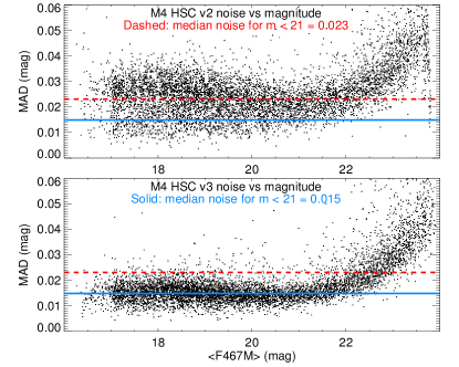
Figure 1: Median absolute deviation (MAD; see Section 4) as a function of the median magnitude in filter F467M in globular cluster M4 for HSC v2 (upper panel) and HSC v3 (lower panel). The plot includes 5300 objects (black dots) that have more than 50 measurements in the WFC3/UVIS F467M filter. The red and blue lines represent the median noise for sources with magnitudes brighter than 21 in HSC v2 and HSC v3, respectively. This field was affected by image alignment problems that have been corrected in HSC v3, which resulted in improved accuracy of the photometry.

The photometric accuracy of HSC v3 is limited by the signal-to-noise of the observations, the accuracy of HST magnitude zero-points, the residual sensitivity variations across the field of view of the instrument, due to imperfect flat-fielding and charge transfer efficiency corrections, and, for the fainter sources, the use of aperture rather than PSF-fitting photometry, which mainly affects crowded fields. For objects with adequate signal-to-noise, the photometric accuracy is generally about 1.5–2%. Figure 1 demonstrates the accuracy in the field of globular cluster M4 and the improvement in HSC v3 compared with the previous release, HSC v2.

1.2 An overview of variability detection techniques

The simplest way of finding variable sources is pair-wise image comparison, used since the early days of photographic astronomy (Hoffmeister et al., 1990). The contemporary approach to image comparison, known as the difference image analysis (DIA; Alard & Lupton, 1998; Bramich et al., 2016; Zackay et al., 2016; Soares-Furtado et al., 2017) is effective in identifying variable sources in crowded fields (e.g. Zebrun et al., 2001; Bonanos & Stanek, 2003; Zheleznyak & Kravtsov, 2003). The intrinsic limitation of the two-image technique is that variations in the source brightness between the images need to be large compared to image noise in order to be detected.

One may use aperture or point-spread function fitting photometry to measure the source brightness on multiple original (or difference) images, constructing the light curve. Using multiple measurements one may identify brightness variations with an amplitude below the noise level of individual measurements. One may test the hypothesis that a given object’s brightness is constant given the available photometric measurements and their uncertainties (Eyer, 2005; Huber et al., 2006; Piquard et al., 2001). This is the standard variability detection approach in X-ray astronomy, where the uncertainties are well known as they are typically dominated by photon noise (Scargle, 1998). The hypothesis testing is less effective for optical and near-IR photometry, as the measurement uncertainties are dominated by the poorly-constrained systematic errors for all sources except the ones close to the detection limit. The scatter of brightness measurements of a non-variable star may be used to estimate photometric uncertainty (Howell et al., 1988; de Diego, 2010) under the assumption that the measurement uncertainties are the same for sources of the same brightness. Relying on this assumption, one may construct various statistical measures of scatter (Kolesnikova et al., 2008; Dutta et al., 2018) or smoothness (Welch & Stetson, 1993; Stetson, 1996; Mowlavi, 2014; Rozyczka et al., 2018) of a light curve to identify variable sources (for a review see Sokolovsky et al. 2017b; Ferreira Lopes & Cross 2016, 2017). Hereafter, we refer to these measures of scatter and smoothness (degree of correlation between consecutive magnitude measurements) as “variability indices” (Stetson, 1996; Shin et al., 2009; Ferreira Lopes & Cross, 2016, e.g.). They are also known as “variability features” in the machine learning context (Kim et al., 2014; Nun et al., 2015; Pashchenko et al., 2018).

Period search is a primary variable star investigation tool and also a very efficient method of variable star identification (Kim et al., 2014; Drake et al., 2014, 2017; Chen et al., 2018). While many types of variable stars show periodic or semi-periodic light variations, photometric errors are expected to be aperiodic, or associated with a known periodic process inherent to the observations (diurnal cycle, periodic guiding errors, orbital period of a space borne telescope, etc.). These spurious periodicities can be identified using the window function (Deeming, 1975). The down side of the period search is that it is computationally expensive, requires hundreds of light curve points for the period search to be reliable (Graham et al., 2013), and excludes the class of non-periodic variables.

To identify specific types of variable objects such as Cepheids, RR Lyrae stars, and transiting exoplanets, one may utilize template fitting. This dramatically increases the search sensitivity to a specific type of variability at the cost of the loss of generality. The sensitivity gain is especially evident for exoplanet transits that typically cannot be identified in ground-based photometry using general-purpose variability detection methods. If templates for multiple variability types are fitted, classification of variable sources is performed simultaneously with their detection (Layden et al., 1999; Angeloni et al., 2014).

The output of multiple variability detection tools may be combined using principal component analysis (Moretti et al., 2018), supervised (Pashchenko et al., 2018) or unsupervised machine learning (Shin et al., 2009, 2012). Machine learning may be applied to design new variability detection statistics (Mackenzie et al., 2016; Pashchenko et al., 2018).

Visual inspection of light curves and images of candidate variables selected using the above methods remains an important quality control tool. It is always applied when one aims to produce a clean list of variable stars (e.g. Pawlak et al., 2016; Klagyivik et al., 2016; Salinas et al., 2018; Jayasinghe et al., 2018) rather than a (more extensive, but contaminated) list of candidate variables (e.g. Oelkers et al., 2018; Heinze et al., 2018). Both types of lists may be useful. Consider two example problems: a) the study of period distributions of W UMa type binaries (which requires confidence in classification of the studied objects as binaries of this particular type) and b) selection of non-variable stars in a given field (to be used as photometric standards or for microlensing studies). In the latter case, it is more important to have a complete list of variable stars, rather than a clean one.

Visual inspection is needed to control various instrumental effects, which produce light curves that are smooth and/or have an elevated scatter. One of the most important effects is the variable amount of blending between nearby sources (e.g. Hartman et al., 2011). The degree of blending may vary with seeing (for ground-based observations), or with the position angle of the telescope if its point spread function (PSF) is not rotationally symmetric (e.g., due to the diffraction spikes produced by spiders holding the telescope’s secondary mirror). If aperture photometry is performed, light from nearby sources may cause additional errors in the position where the aperture is placed over the source in a given image, which can lead to large errors in the measured source flux. Depending on the optical design of the telescope, slight focus changes may have noticeably different effects on the PSF size and shape depending on the source color (e.g. Sokolovsky et al., 2014). The amount of blending may also change if one of the blended sources is variable. Other effects that may corrupt photometry of an individual source include the various detector artifacts (hot pixels, bad columns, cosmic ray hits) or the proximity to the frame edge/chip gap. Uncorrected sensitivity variations across the CCD (due to imperfect flat-fielding and charge transfer inefficiencies) coupled with the source image falling on different CCD pixels at different observing epochs may produce artificial variations in a light curve. If the sensitivity varies smoothly across the CCD chip affecting nearby sources in a similar way, one may try to correct the light curves for these variations using algorithms like SysRem (Tamuz et al., 2005), a trend filtering algorithm (Kovács et al., 2005; Kim et al., 2009; Gopalan et al., 2016), or local zero-point correction (Section 3).

In this paper, we describe the HCV system and catalog resulting from a systematic search for variable objects in the HSC v3. It should be noted that “HCV” can either refer to the processing system (i.e., the development of the hardware, software system and pipeline to create the catalog) or the catalog itself. The paper is structured as follows: Section 2 presents an overview of the HCV system developed to identify variable sources in the HSC. Section 3 describes the preprocessing applied to the HSC photometry, while Section 4 describes the algorithm for selecting candidate variables. Section 5 presents the algorithm adopted for validating the candidate variables. Section 6 presents the performance and limitations of the HCV catalog, while Section 7 outlines the statistics of the HCV catalog and highlights some scientific results. A summary is given in Section 8.

2 HCV system overview

The HCV processing system aspires to identify all the variable and transient sources in the HSC through simple mathematical techniques, thus producing the HCV catalog.

The sole data input to the HCV pipeline is the HSC, which provides a set of tables containing specific information about the individual sources observed by the HST instruments at different epochs. The HSC is naturally divided into groups of sources detected on overlapping HST images (Whitmore et al., 2016). Each group was assigned a unique GroupID identifier. Within the group, observations of the same source are identified and combined into a “matched source” to which another unique identifier is attached (MatchID). The observations of a matched source, hereafter simply mentioned as “a source”, over all available epochs form the input to the HCV pipeline.

The HCV catalog is generated by a pipeline that consists of the following stages of operation:

• importing and organizing the HSC data in a form that facilitates processing for variability detection,

• detection of candidates for variability, after applying specific limits on the data quality and quantity, rejecting inappropriate sources within a group and even groups (see Section 6.2),

• validation of the detected candidates using an automated algorithm,

• extraction of source and variability index (Sec. 1.2) data for all the processed sources (candidate variables and non-variables),

• curation of candidate variable sources and expert validation,

• publication of the resulting catalog datasets into publicly available science archives, specifically, the ESA Hubble Science Archive, eHST (ESAC), and the Mikulski Archive for Space Telescopes, MAST (STScI).

In the following subsections we describe the (largely configurable) components of the HCV system, which supports this computationally intensive process and forms a pipeline of distinct data fetching, processing, and depositing.

2.1 System concept

The HCV system, at the highest level, consists of three functional sub-systems: (a) DPP, the data processing pipeline (hcv.dpp), which deals with the computational requirements of the system, employing distributed infrastructure for processing and data storage; (b) CAT, the (mostly) relational data driven HCV catalog sub-system (hcv.cat) where typical expert driven data management and curation operations are performed; (c) an interface to specific science archives (hcv.bridge). Furthermore, there is a fourth enabling element, the infrastructure (hcv.infra) that manages the security and access, monitoring, logging, and other non-functional aspects of the system. The top-level architecture of the system is illustrated in Figure 2 and the major elements of the HCV system and their functions are listed in Table 2.

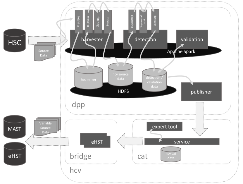
Figure 2: HCV system high-level architecture, showing three major components (dpp, cat, bridge) and their elements. These components correspond to the top-level functional subsystems of the HCV system.

Table 2: HCV system functional components.

HCV component	Function
hcv.dpp	data processing pipeline
hcv.dpp.harvester	interface to the HSC archive tables
hcv.dpp.detection	detection of variables
hcv.dpp.validation	validation of candidate variables
hcb.dpp.publisher	publication of source data to catalog
hcv.cat	HCV catalog subsystem
hcv.cat.service	HCV database service layer
hcv.cat.ui	HCV expert tools for curation
hcv.bridge	system interfaces to external archives
hcv.bridge.mast	STScI archive component
hcv.bridge.ehst	ESAC archive component
hcv.infra	infrastructure enabling layer
hcv.infra.management	infrastructure management tools
hcv.infra.monitoring	operation monitoring subsystems
hcv.infra.logging	logging subsystem
hcv.infra.security	authentication / authorization

The data processing pipeline (hcv.dpp) hosts the computationally and data intensive processes of the HCV system. It utilizes high performance distributed processing and storage technologies and employs highly configurable algorithms for its operations, which may be fine-tuned or even replaced to fit future needs of the HCV system. Its elements are:

• hcv.dpp.harvester - enables access to the external HSC archive.

• hcv.dpp.detection - applies the variability detection algorithm, estimates parameters that characterize variability (i.e., variability indices), and identifies candidate variables.

• hcv.dpp.validation - provides tools to analyze and verify and/or validate the variable candidates. It applies the variability validation algorithm and validates candidates as variable sources.

• hcv.dpp.publisher - ingests the outcome of processed data into the HCV relational database.

The objective of the harvester is to retrieve sources and their metadata from the HSC database and transform those data into a form efficient for further processing, according to the requirements of the HCV data model. The harvester utilizes a compressed, columnar data format and parallel processing of the HSC data. In order to save space, the harvester may opt to completely omit specific portions of the HSC (e.g., single epoch observations). A significant feature of the harvester is its configurability to adapt to changes in HSC data structures.

The detection and validation elements implement the data processing pipeline. Initially, the extremely large groups are split into a number of clusters (hereafter referred to also as ”subgroups”), based on source coordinates. The sources that are nearby on the sky tend to be assigned to the same cluster. This clustering procedure is based on the k-nearest neighbors algorithm (k-NN) and is necessary to satisfy the CPU requirements of the core algorithms, and enable sufficient parallelization of the process, as the element of work is the cluster, which may be an entire HSC group (GroupID). Next, the HSC photometry is preprocessed (see Section 3) in order to remove unreliable measurements and apply local zero-point corrections. The light curves are constructed by retrieving the (corrected) photometric measurements obtained with the same instrument and filter combination at different epochs for all sources in each subgroup. The pipeline then computes the magnitude scatter in each light curve, the variability indices, and applies a magnitude-dependent threshold to select candidate variable sources (Section 4). Finally, it applies an automated validation algorithm to the candidate variables in order to remove obvious false-detections (see Section 5).

The last step of the pipeline, the publisher, implements a Representational State Transfer (REST) web service interface. It ingests all data delivered by the detection and validation components into the HCV database, that is each and every candidate and non-candidate variable source processed. This dataset is the HCV catalog.

The catalog sub-system (hcv.cat) is a typical web application component that enables inspection and validation of the outcome of the pipeline. It is based on fundamentally different technologies and employs a relational database management system to contain its data structures. It consists of two elements:

• hcv.cat.service - provides a REST web service abstraction layer over the HCV database, covering all functionality for data management, such as create-read-update-delete operations, data publication, and authentication/authorization.

• hcv.cat.ui - offers a tool for highly streamlined expert-driven data validation of the catalog data.

The last subsystem of the HCV system, the hcv.bridge, provides the external science archives with access to the publishable release of the HCV catalog. The latter is exported via the bridge adapters in a fixed open format, JSON (JavaScript Object Notation), utilized by the targeted archives.

Furthermore, additional tools are provided to facilitate data inspection and handling, which are particularly useful during algorithm fine-tuning and exploration of the HSC. One of the tools utilizes the temporary outputs of the pipeline supporting the algorithm validation and configuration phase. The tool allows experts to inspect the light curves and other information available for the candidate variables in order to identify issues prior to producing the catalog, as well as to evaluate the success of the pipeline. The second tool operates on the data imported from the pipeline to the database allowing for validation by experts, which is optional. It enables fine grained manipulation, updating of a particular dataset, freezing and/or publishing the catalog and exporting it in native format.

2.2 Implementation technologies

The main driver behind our choice of technologies for the HCV system implementation was the large amount of input, intermediate and output data (see Table 3), and, correspondingly, the large-scale data processing. An additional driver was the nature of the source processing. Although there is a discrete sequence of steps, that is HSC ingestion, variable candidate detection and validation, publication to the catalog, and catalog operations, there are processes within most of these steps that can run in parallel. This is because either these sub-stages are independent or because one set of data can be processed independently of another (groups or subgroups). The portability of the system was important in order to allow different infrastructures to be developed and deployed, as well as to avoid “vendor lock-in”. The ability of the system to utilize resources that are offered to it (e.g., CPU and RAM) is the cornerstone of the scalable design and technologies implemented for the HCV system.

Essentially the whole HCV system relies on Free Open Source Software (FOSS). The following list presents the most essential elements:

• Linux is the operating system of the infrastructure, providing many of the baseline services required for operating the infrastructure.

• Hadoop Distributed File System (HDFS) is the distributed, high-throughput file system employed for storing the non-relational data of the system.

• Apache Spark is the distributed parallel processing platform, which allows the system to carry out its computationally intensive tasks exploiting all resources provided to it. Apart from implementation of Spark-enabled algorithms, DPP uses specific Machine Learning elements (clustering) provided in the Spark ecosystem.

• Mesos is the hardware abstraction layer over which Apache Spark operates.

• Apache ZooKeeper is utilized for centralized configuration management and synchronization of services of the system.

• Apache Parquet is the columnar format employed over HDFS to provide storage and access features for DPP processes.

• PostgreSQL is the relational database management system that hosts the HCV catalog data component.

• Java is the platform for the implementation of the components of the system supported by several Java ecosystem technologies such as Hibernate, Spring Framework, Tomcat etc.

2.3 Deployment and performance

The system is deployed on a virtualized Intel x64 architecture, yet there are no particular dependencies on this architecture. It has been successfully operated over XEN, VMware, and Hyper-V hypervisors.

In operational deployment at STScI, the HCV pipeline is provided with four worker nodes, each consisting of 16 virtual cores and 64 GB RAM, and shared HDFS storage of over 10 TB. Those can be easily up-scaled to larger numbers if required. Two additional nodes, one consisting of four virtual cores and 16 GB RAM, the other of eight nodes and 32 GB memory, are dedicated, respectively, to (a) operation of the infrastructure and several enabling components, such as the code repository and (b) the hosting of the hcv.cat and hcv.bridge subsystems for the handling and publication of the catalog of variables.

Over this infrastructure, the processing of the HSC v3 was carried out. Performance data are presented in Table 3; the total duration of the run is about ten days. We note that the processing times in Table 3 are indicative, as they heavily depend on network and VM load and have been observed to deviate by more than 100% during peak hours.

Table 3: Performance of the HCV system processes in operational deployment at STScI.

Process	Product	Type	Size	Duration
Download	HSC tables	CSV-files	1.9 TB	12h 45m
Harvesting	HCV tables	parquet	700 GB	02h 48m
Input	HCV input	parquet	38 GB	00h 20m
Clustering	HCV input	parquet	38 GB	02h 47m
Det.&Valid.	DPP output	JSON	80 GB	17h 40m
Import DB	CAT dataset	SQL	80 GB	7 days
Export CAT	HCV export	JSON	0.5 GB	00h 15m

3 HSC photometry preprocessing

The task of identifying variability in a photometric light curve requires a reliable and clean dataset. As HST is not a survey telescope, it performs observations that are specifically designed for each individual project, using diverse filters, exposure times, pointings, and dithering patterns. Consequently, the uniform reduction and photometry provided by the HSC cannot address issues specific to certain datasets as well as a tailored reduction of each dataset. It can thus, inadvertently, introduce systematic effects in the photometry. Furthermore, cosmic ray hits, measurements near the edge of the CCD or in a region with nebulosity etc. can also introduce systematic effects. Therefore, before proceeding with the variability search described in Section 4, we apply quality cuts and additional photometric corrections to the input HSC data. The procedure described below was developed from a comprehensive investigation of the “Control Sample” fields (see Section 6) and numerous randomly selected fields from different instruments, initially with data from the HSC v1, and subsequently with data from the HSC v2 and HSC v3, as the new releases became available. The procedure was eventually applied to the whole HSC v3.

3.1 Light curve data collection

We adopted the following procedure to construct light curves of HSC v3 sources. We used the HSC parameter GroupID, which indicates a group of overlapping white-light images (corresponding to Level 2 ”detection” images of the HLA), to select observations of sources in a specific field. We consider only the groups that have at least 300 detected sources (N${}_{\rm sources}\geq 300$) and only the sources that have at least five detections ($n_{\rm LC}\geq 5$) with the same instrument and filter combination. These constraints should ensure the reliable operation of the variability detection algorithm described in Section 4. We also applied cuts on the following HSC parameters (for a detailed description see Whitmore et al., 2016):

• The Concentration Index (CI), defined as the difference between the source magnitude measured in two concentric apertures (see aperture sizes in Table 1 of Whitmore et al., 2016), was limited to $\texttt{CI}=\texttt{MagAper1-MagAper2}<5.0$. The CI is a measure of the spatial extension of a source and can be used to identify sources potentially affected by light from their neighbors (blending, diffraction spikes from bright stars, a diffuse background) or cosmic rays. Typically, real extended sources have $\texttt{CI}\approx 2-4$ mag, while larger values of CI usually indicate problematic photometry or image artifacts.

• Magnitude cuts of $\texttt{MagAper2}<31.0$ and $\texttt{MagAuto}<35.0$ mag were used to remove unphysical measurements.

• The photometric error MagerrAper2 estimated by SExtractor, which provides a lower limit on the total photometric uncertainty, was used to eliminate uncertain measurements by adopting $\texttt{MagerrAper2}\leq 0.2$ mag. This value is a conservative, typical error adopted from the faint end of the magnitude.

• SExtractor and HSC flags were constrained to $\texttt{SE\_flags}\leq 7$ and $\texttt{Flags}<4$, respectively, to exclude objects flagged as truncated, incomplete/corrupted, or saturated. We cannot rely on the SExtractor saturation flag, as the CCD saturation limit is not always propagated properly to the white-light images.

• Sources with undefined (null) values of the above parameters were also rejected.

After applying all the quality cuts described above, light curves from the same instrument and filter combination were constructed for each source, which is identified by its unique MatchID in the HSC catalog.

3.2 Light curve filtering and outlier identification

During the construction of the HCV pipeline, we identified several issues with the HSC photometry including misalignment between images in a visit stack, background estimation problems resulting in corrupted photometry of sources close to the image edges (“edge effect”), issues regarding local correction, saturation, double detection, and so on. Several of these were corrected or improved in the HSC v3, although some continue to affect the HSC photometry and therefore the HCV catalog (see Section 6.2). Additional light curve filtering was therefore required to reduce the false detection rate of candidate variables.

The filtering performed during the preprocessing included the following main steps: identification and flagging of photometric outliers, identification and rejection of “bad” images that produce many photometric outliers, local magnitude zero-point correction, and identification and rejection of additional unreliable data points that have large synthetic errors (defined below). Four parameters were used to evaluate the quality of the HSC photometry:

1. MagerrAper2.

2. CI.

3. The offset distance D of a source from its average position listed in the catalog (“match position”), as an uncleaned cosmic ray or misalignment between images in the white-light stack will change the center of light (pixel-flux-weighted position of the source) and corrupt its photometry.

4. The difference between the source magnitude measured using the circular (MagAper2) and the elliptical aperture (MagAuto), MagAper2-MagAuto. This difference is expected to be constant for isolated sources. For a close pair of sources that were not resolved by SExtractor, the elliptical aperture may include both sources, while the circular aperture may include only one.

We assigned a weight to each light curve point that is inversely proportional to the square of the quantity we defined as the “synthetic error”:

$$Error_{syn}=\sqrt{\begin{aligned} &\left(\frac{\texttt{MagerrAper2}}{{<\texttt{MagerrAper2}}>}\right)^{2}\\ &\qquad+\left(\frac{\texttt{CI}}{<{\texttt{CI}}>}\right)^{2}+\left(\frac{D}{<{D}>}\right)^{2}\\ &\qquad+\left(\frac{\texttt{MagAper2}-\texttt{MagAuto}}{<{\texttt{MagAper2}-\texttt{MagAuto}}>}\right)^{2}\end{aligned}}\qquad,$$ (1)

where ${<}X{>}$ indicates the median value of each parameter of the light curve. When parameters were not available (which most commonly occurs when a flux in one of the apertures is negative), they were set to zero. The synthetic error was used to identify data points that differ from the rest of the measurements for each object. In principle, the synthetic error could be used on its own to identify bad measurements. However, due to the image misalignment problem and uncertainties of the parameters (which may result in some outliers with normal synthetic error), the synthetic error had to be combined with additional outlier-rejection steps.

A weighted robust linear fit (Press et al., 2002) was performed for each light curve, using the synthetic error to set relative weights of the light curve points instead of the photometric error. The fit was used to obtain the scatter of measurements, the robust sigma ($\sigma^{\prime}$; a resistant estimate of the dispersion of a distribution, which is identical to the standard deviation for an uncontaminated distribution), around the best-fit line and mark outlier points deviating by more than $3\sigma^{\prime}$ from that line. The “potential outliers”, with magnitude measurements within $3\sigma^{\prime}$ but having their synthetic error $>4\sigma_{syn}$ were also marked at this step. The $\sigma_{syn}$ was calculated in a similar way to $\sigma^{\prime}$, but instead of using a linear fit, the median value was adopted, since the components are expected to be constant and to be measured in the same way, unless external contaminating factors exist.

By comparing the light curves of all sources in a given subgroup, we identified visit-combined images having $>20\%$ of their sources marked as outliers. These visits were marked as “bad” and all measurements obtained during these visits (not only the ones marked as outliers) were considered unreliable and discarded from the analysis. This was found to be a very efficient way of identifying corrupted images. Once the bad visits were removed from the dataset, the robust linear fit was repeated as the removal of a bad visit may have changed the $\sigma^{\prime}$ values.

The magnitudes predicted by the robust linear fit for each visit were used to compute the local zero-point corrections (e.g. Nascimbeni et al., 2014). For each source we used other HSC sources within a radius of 20^′′ around it to compute the correction. For each visit we calculated the magnitude zero-point correction for a given source as the median difference between magnitudes predicted by the linear fit and the ones measured for the nearby sources that have measurements in the same visit that are not marked as outliers or potential outliers (i.e., having ¡$3\sigma^{\prime}$ and ¡$4\sigma_{syn}$). This correction should be able to eliminate the photometric zero-point variations from image to image and from one area of the chip to the other (as long as the spatial variation of the zero-point is sufficiently smooth), and also the effects of thermal breathing of the telescope, changing of PSF, for which the total flux difference from visit to visit can reach up to $\sim$6% (Anderson & Bedin, 2017). It may also partly compensate for any residual charge transfer inefficiencies (Israel et al., 2015) that remain after the corrections that were applied at the image processing stage.

After the local correction was applied, the robust linear fit was performed again as the local correction (just as the bad visit removal above) may change the $\sigma^{\prime}$ values. We flagged all the outliers and potential outliers in all light curves and discarded them from further analysis in order to reduce the rate of false detections among the candidate variables. While application of the local zero-point correction considerably improved light curve quality, the procedure cannot correct the extreme outliers. These outlier measurements are associated with poor quality images and with cases where photometry of an individual star, rather than a group of nearby stars, is corrupted by an image artifact. Figure 3 presents an example of the preprocessing procedure applied to a light curve in M4. We note that the outliers were removed by the preprocessing in an iterative process. Also, the systematic offset between different visits was removed, which reduced the light curve scatter.

The data preprocessing techniques used for the production of the HCV catalog can be applied to any other time-domain survey, following a careful evaluation of the dataset. Remaining issues, which correspond to limitations and caveats of the HCV catalog, are described in Section 6.2.

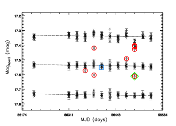
Figure 3: Light curve of a source in the field of M4 (MatchID=27382770; WFC3_F775W filter), demonstrating the application of the preprocessing procedure. The figure shows the original light curve retrieved from the HSC (top), the local-corrected light curve (middle), and the final cleaned light curve (bottom). For clarity, the light curves are offset by 0.2 mag. In each step of the procedure, the outliers (¿$3\sigma^{\prime}$; red circles) and potential outliers (¡$3\sigma^{\prime}$ and ¿$4\sigma_{syn}$; blue squares) are marked. Outliers that also have a large synthetic error (¿$4\sigma_{syn}$) are marked by green diamonds.

4 Algorithm for detecting candidate variables

Our goal is to recover all variable objects that can in principle be recovered from each dataset in the HSC v3. The efficiency of the HCV pipeline in finding variable objects should be limited by the input data, not by the processing algorithm.

We require a general-purpose variability detection algorithm that is robust to individual outlier measurements, applicable to a wide variety of observing (sampling) cadences and efficient in detecting a broad range of variability patterns, including periodic and non-periodic ones, rapidly and slowly varying objects, and transients visible only on a small subset of images of a given field. Taking into account the heterogeneous nature of the input HSC v3 data, we tested various statistical indicators of variability (“variability indices”, Section 1.2), which characterize the overall scatter of measurements in a light curve and/or degree of correlation between consecutive flux measurements.

Sokolovsky et al. (2017b) presented a detailed description and comparison of 18 variability indices proposed in the literature. These indices were tested on seven diverse sets of ground-based photometric data containing a large number of known variables. Simulated data were also used to investigate the performance of the indices based on the number of points in a light curve. The authors concluded that for light curves with a small number of points, the best result is achieved with variability indices quantifying scatter (such as the interquartile range and median absolute deviation). This study resulted from the development phase of the HCV variability detection algorithm and the search for the optimal variability indices for the HSC data. We complement this study with simulations based specifically on the HSC data, which are described in Appendix A.

We adopted the median absolute deviation (MAD) as the robust variability index for the HCV detection algorithm. The MAD is defined as

$${\rm MAD}={\rm median}(|m_{i}-{\rm median}(m_{i})|),$$ (2)

where $m_{i}$ is the magnitude of $i$’th point in the light curve. This index is robust to individual outlier measurements and sensitive to a broad range of variability types. In a five-point light curve, up to two points may be completely corrupted without compromising the MAD value. The interquartile range (IQR), another robust variability index discussed by Sokolovsky et al. (2017b), is less robust to outliers in the extreme case of a five-point light curve: it will be able to tolerate one or zero outlier points depending on the exact implementation. According to our simulations described in Appendix A, MAD is more efficient than the IQR in a data set heavily contaminated with outlier measurements when the number of light curve points in small ($n_{\rm LC}<10$).

For each HSC group and for each filter, the HCV pipeline constructs a diagram of the median magnitude of each source versus the value of MAD for its light curve. The candidate variables are identified as the sources having a MAD value above a magnitude-dependent $5\sigma$ threshold. Figure 4 presents an example from the Control Sample field IC 1613 (see also Table 4). The location of the selected variables on the color-magnitude diagram is also shown.

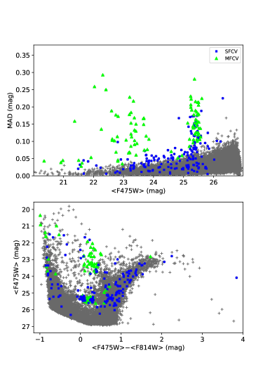
Figure 4: Upper panel: MAD vs. median ACS_F475W magnitudes for all sources in the Control Sample field IC 1613, shown with gray crosses. The multi-filter variable candidates (MFVCs) are marked with green triangles, while the single-filter candidates (SFVCs) are marked with blue squares. SFVCs that have low MAD values in the F475W filter were selected as having MAD values above the threshold in the F814W filter. Lower panel: Color-magnitude diagram for IC 1613 showing the location of the MFVCs and SFVCs in the field. Many of the candidate variables lie on the instability strip.

The magnitude-dependent threshold was calculated for each subgroup in each filter as follows. First, the sources were ordered in magnitude. We rejected sources within 0.2 mag of the faintest source as they may be affected by background estimation inaccuracies and residual cosmic rays. We similarly rejected sources within 0.5 mag of the brightest star, to avoid saturation problems. The usable range of magnitudes varied depending on the gain setting of the camera. We divided the range into 20 overlapping bins in magnitude and calculated the median and clipped $\sigma$ values of MAD for each bin. The MAD value of each source in the bin was compared to the threshold ${\rm median}({\rm MAD})+5\sigma$ (where the median is computed over the MAD values of all sources within that bin) and sources above the threshold were marked as variable. The pipeline continued to the next bin, but also included 30% of the sources from the previous bin so that the bins were overlapping. A source located in an overlapped bin was marked as variable if it was above the threshold in at least one of the bins. The candidates having large photometric errors (as estimated by SExtractor) were rejected at this stage by requiring the value of reduced ${\chi^{2}>3}$ for the null-hypothesis of the source magnitude being constant. The outcome of the detection algorithm was a list of candidate variables, which was input to the validation algorithm described in the following section.

The above algorithm failed in the rare cases where the majority of stars in a magnitude bin were actually variable. In such cases, the calculated threshold was too high and some real variables failed to pass it. The dwarf galaxy Eridanus II (GroupID 1075853) is an extreme example for this situation. Here, no RR Lyrae variables were detected as they all occupy a narrow magnitude range (being horizontal branch stars, all at the same distance).

5 Algorithm for validating candidate variables

The candidate variables that were identified by the application of the variability detection algorithm (Sec. 4) were evaluated and further characterized by the DPP using a validation algorithm. This algorithm applied a series of criteria leading to variability quality flags assigned to each candidate variable. Furthermore, expert validation was conducted for a random subset of groups to evaluate the performance of the HCV pipeline. Although we implemented and tested several period finding algorithms in the HCV pipeline, they did not yield useful results, given the inhomogeneous cadence and small number of epochs of the HCV light curves (typically having less than ten points), and were therefore turned off in the final version of the pipeline.

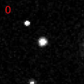
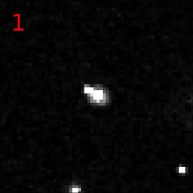
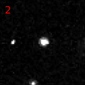
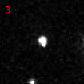
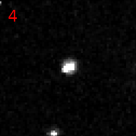
Figure 15: WFC3 images of HSC v3 source with MatchID=45740877 (centered) corresponding to the measurements highlighted in red in Fig. 12. Images 1–4 show obvious distortions of the object’s shape due to uncleaned cosmic ray hits, resulting in outlier photometric measurements (Fig. 12). Image 0 is an example of a measurement unaffected by a cosmic ray hit. We note the additional uncleaned cosmic rays in images 0–2.

Initially, the validation algorithm determined the number of filters for which a variable candidate displayed variability. If variability was detected in more than one filters, then the candidate was classified as a “multi-filter variable candidate” (MFVC), otherwise it was classified as a “single-filter variable candidate” (SFVC). The SFVCs include two different classes: (a) sources for which there are data available only in one instrument and filter combination, (b) sources for which there are data in more than one instrument and filter combinations, but variability was detected only in one of them. One might assume that these variable candidates are less reliable. However, the two major classes of variables in the HCV catalog, namely Cepheids and RR Lyrae variables (see Section 7) have a larger amplitude in the blue than in red, so some of them may not be detected in the redder filters. Also, there are cases where the quality of the photometry is much worse in one instrument and filter combination, which may also affect the variability detection. The remaining sources that showed no significant variability were classified as “constant sources”. In addition, a “variability quality flag” was assigned to each candidate variable. This variability quality flag aims to quantify the variation of the source image characteristics between visits, given that a corrupted photometric measurement may be associated with a noticeable change in the source image shape (e.g., Fig. 15).

The parameters used to assign the variability quality flag are the concentration index CI, the offset distance D-parameter, MagerrAper2, the difference between MagAper2 and MagAuto, which have been defined in Section 3, and the peak-to-peak amplitude (p2p) in the light curve. For each source and each light curve point there is one value for each of these parameters. We derived the standard deviation for each of these parameters and for each source light curve, $\sigma_{par,i}$, where $i$ signifies the $i^{th}$ source. We also constructed the distribution of $\sigma_{par,i}$ for all sources lying in the same magnitude bin as the source in question, whether they are variable or not. This distribution is fit with a gaussian function and the mean value and standard deviation ($\sigma_{dist}$) were calculated. The amount by which $\sigma_{par,i}$ differs from the average value within the magnitude bin is indicative of the quality of the photometric data for the specific source compared to other sources of similar brightness in this subgroup. For example, if $\sigma_{\texttt{CI},i}$ for a particular source is much higher than average, the source is probably blended.

Based on these parameters, we constructed a variability quality flag, which consists of five letters and quantifies the deviation of each parameter from the average behavior within the subgroup. Each flag can obtain the values A (highest quality), B, or C (lowest quality). In the HCV output, the flags are ordered as follows: CI, D, MagerrAper2, MagAper2-MagAuto, p2p. The assignment of values A, B, and C depends on the deviation of a value from the average. The criteria for the first four parameters are defined as follows:

• value A: $|\sigma_{par,i}$– $\overline{\sigma_{par}}|<3\sigma_{dist}$

• value B: $3\sigma_{dist}\leq|\sigma_{par,i}$–$\overline{\sigma_{par}}|<5\sigma_{dist}$

• value C: $|\sigma_{par,i}$– $\overline{\sigma_{par}}|\geq 5\sigma_{dist}$.

For the p2p parameter, the values A, B, C, are defined as follows:

• value A: $|\sigma_{p2p,i}$– $\overline{\sigma_{p2p}}|\geq 5\sigma_{dist}$

• value B: $3\sigma_{dist}\leq|\sigma_{p2p,i}$–$\overline{\sigma_{p2p}}|<5\sigma_{dist}$

• value C: $|\sigma_{p2p,i}$– $\overline{\sigma_{p2p}}|<3\sigma_{dist}$.

A comparison of flag values to expert-validated variables (see next Section) shows that a candidate is more likely to be a true variable if there are at least 3A’s in the quality flag and if the D-parameter and MagAper2-MagAuto have a quality flag A. However, there were cases where the pipeline was not able to evaluate one or more of the parameters (denoted by a ”dash” in the variability quality flag), for example, when SExtractor returned a negative flux or when $\sigma_{dist}$ was very small and its value was rounded to zero. The latter occurred when the number of sources per bin was small.

5.1 Expert validation

The variable candidates produced by the pipeline were individually evaluated by “expert users”, using an “expert tool” interface developed for this purpose. Due to the large number of candidates and time constraints of the project, only the multi-filter variable candidates and a random sub-sample of single-filter candidates were visually inspected. It is noted that the experts flagged 25 subgroups as unreliable because they presented a large number of artifacts (see Section 6.2). These unreliable groups contained around 50% of the multi-filter variables identified by the pipeline. The results of the expert validation are discussed in Section 7. The majority ($\sim 75\%$) of the remaining multi-filter variables were expert validated by three experts, while the single-filter variables were validated by one expert. The expert-validated variables, and in particular the multi-filter variable candidates are considered highly reliable.

The expert users inspected the “discovery diagram” (MAD versus magnitude, with the calculated thresholds used for variable selection), the light curves of a specific candidate variable, its location on the color-magnitude diagram (when magnitudes in at least two different filters were available), the variations of CI and D as a function of time, the variability quality flag and the appearance of the candidate on three image “stamps” (corresponding to the faintest, brightest and median points in the source light curve) downloaded from the HLA. Taking into consideration all the different diagnostics, the expert classified a candidate as a “high-confidence variable”, a “probable variable”, or a “possible artifact”. It must be noted that the expert validation relies heavily on the inspection of the three stamp images. Low amplitude variability (less than 0.5 mag) is difficult to assess by eye, especially when no neighboring comparison sources are visible on the same stamp. Therefore, it is possible that a low amplitude or an isolated source is not confirmed as a high confidence variable by an expert, while it may actually be variable. Therefore, a significant percentage of the “probable variables” are likely true variables.

The classifications by the expert users were merged using a simple voting algorithm. If one of the three outcomes had a majority vote – it was accepted as the final result. If there was one vote for “high-confidence variable” and one for “possible artifact” then the result was “probable variable”. If there were equal votes for “probable variable” and “possible artifact”, or “probable variable” and “high-confidence variable”, then we accepted the “possible artifact” and “high-confidence variable” result, respectively. The expert classification is included in the HCV catalog as an additional flag.

The expert validation procedure was very useful in discovering and discarding spurious candidate variables. In most cases, such spurious variables originated from the proximity of the source to very bright stars and their diffraction spikes, or from blended sources, objects projected on a highly spatially variable background, extended and diffuse objects (e.g., galaxies) where small noise-induced variations in aperture centering induce false variability, and other issues, such as image misalignment (see Section 6.2 for a full list of caveats).

6 Performance and limitations

The performance of both the validation and the variability detection algorithms was monitored using ten representative HST fields, constituting the “Control Sample”. These fields have been previously searched for variables in dedicated, published studies. The Control Sample includes a globular cluster, galaxies of the Local Group, more distant resolved galaxies, and a deep field. The comparison between the detected (by the detection and validation algorithm) and documented (in the literature) variables in the Control Sample led to the identification of possible problems and to necessary revisions and refinement of both algorithms.

Table 4: Properties of the HCV Control Sample fields.

Field	Distance	Instrument	Filters	${\Delta_{\rm MJD}}^{a}$	# visits	$N_{\rm sources}$	# known	Recovery	Type of	Referenceb
Name				(days)			variables	rate (C)	variables
M 4	1.86 kpc	WFC3	F467M,	300	100	8,460	38	0.32	RR Lyr,	1
			F775W						EB
IC 1613	760 kpc	ACS	F814W,	3	12	23,106	182	0.71	RR Lyr,	2
			F475W						Cepheids,
									EB
M31-Halo11	770 kpc	ACS	F814W,	40	32	10,059	115	0.80c	RR Lyr,	3
			F606W						Dwarf Cepheids,
									LPVs,
									semiregulars
M31-Stream	770 kpc	ACS	F814W,	30	16	6,792	24	0.88	RR Lyr	4
			F606W
M31-Disk	770 kpc	ACS	F814W,	39	15	10,644	23	0.83	RR Lyr	4
			F606W
M101-F1	6.4 Mpc	ACS	F814W,	$>$30	14	58,263	411	0.80	Cepheids	5
			F555W
NGC 4535	16 Mpc	WFPC2	F814W,	75	14	1,032	50	0.09	Cepheids,	6,7
			F435W						supergiants
M 87	16.5 Mpc	ACS	F814W	30	48	15,731	32	0.63	Novae	8
NGC 1448	17.3 Mpc	WFC3	F350LP,	50	11	9,228	54	0.44	Cepheids	5
			F160W
GOODS-S		ACS	several	50 to	5 to	14,278	116	0.26	AGN,	9
		WFC3		3000	120				SNe

The Control Sample fields were selected from HSC v1, which was available during the early development phase of the HCV project, on the basis of the following requirements:

• Availability of accurate astrometry for the known variables

• Coverage of as wide a range of input data characteristics as possible, namely, a wide range in the number of visits, source number densities, numbers and types of known variables, distances, as well as instrument and filter combinations.

Table 4 presents the characteristics of each Control Sample field: the name of the field, the average distance of the sources in the field (when applicable), the instrument(s) and filter(s) used, the time baseline of the data, calculated as the difference in the Modified Julian Dates (MJD) of the start and end of the observations, the median number of visits (since not all sources belonging to the same GroupID have the same number of visits), the total number of sources, the number of published variables, the completeness, C, of the recovered published variables, that is the ratio of the number of detected candidate variables over the number of published variables that are included as sources in the HCV catalog sample, the type of published variables, and the corresponding reference(s).

After selecting the fields appropriate for the assembly of the Control Sample, astrometric corrections were estimated and applied to the published coordinates of the variables in each field, where necessary, in order to make cross-matching with the HSC possible. Indeed, many published HST variables lack proper astrometry, while only pixel coordinates (with or without finding charts) are provided by some authors. For example, we found offsets as large as 5$\arcsec$ between published (Bernard et al., 2010) and HSC coordinates for sources in IC 1613.

Although care has been taken for the Control Sample to be as representative as possible, it is clear that there are several cadence profiles that one may encounter in the HSC, but not in published data. In order to better characterize the variability detection efficiency we use simulations injecting artificial variability into real HSC light curves and then reduce the number of points by randomly removing observations. The simulations are described in Appendix A. They show that the efficiency of variability detection increases dramatically with the number of light curve points increasing from five to ten. For the larger number of points, the efficiency continues to rise, but more slowly (Fig. 13, Fig. 14). This result is valid for the situations where the variability timescale is shorter than the time difference between consecutive light curve points.

6.1 Recovery of known variables

The Control Sample fields were used to evaluate the performance of the variability detection and validation algorithms and the limitations present. The recovery rates C (defined as the ratio of variables identified by the pipeline over the total number of known variables) presented in Table 4 vary from 9% for NGC 4535 (WFPC2) to 88% for the M31-Stream (ACS) field. The recovery rate generally depends on the type of variable, the distance of the field studied, and the number of epochs available. WFPC2 systematically yields a lower recovery rate due to the lower data quality. Other conditions affecting the recovery rate include fields that are close enough for proper motions to cause a deterioration of the localization of the sources (e.g., Galactic bulge fields), fields that have several bright stars in their field of view (e.g., globular clusters), and extended sources (distant galaxies), where robust source centering is not possible.

Generally, high-amplitude periodic variables are more easily detected, depending on the cadence of the observations. The use of visit-combined photometry adopted in the HSC, reduces the effective number of available epochs and often limits the detectability of fast variability, for example, eclipsing binaries (EB; with short duration of eclipses). This is the case for M4, where the majority of the variables are eclipsing binaries (the low recovery rate for the M4 field is also affected by blending issues and the presence of several bright stars with diffraction spikes). The reduction of available epochs may also affect the detection of transients. Additionally, the use of aperture rather than PSF photometry does not yield high quality photometry in more distant and/or crowded fields. A detailed description of the caveats in the HCV catalog is provided in Section 6.2.

The only Control Sample field using WFPC2 is the HST Key Project (Freedman et al., 2001) galaxy NGC 4535, which is known to host 50 Cepheids (Macri et al., 1999). Spetsieri et al. (2018) performed PSF photometry using DOLPHOT on the archival images of the galaxy, and applied variability indices to recover the 50 known Cepheids and 120 additional candidate variable stars. The HCV catalog includes eight of the known Cepheids and 11 of the additional candidate variables. The differences in recovery rate and identification of variables are due to the fact that the HSC v3 source lists for WFPC2 are not very deep and that the particular field is crowded. This field demonstrates the limitations of the HCV catalog results in crowded fields observed with WFPC2 (see also Section 6.2). Future releases of the HSC are expected to improve on the quality and depth of the WFPC2 source lists.

Spetsieri et al. (2019) similarly analyzed WFPC2 data of the Key Project galaxies NGC 1326A (Prosser et al., 1999), NGC 1425 (Mould et al., 2000), and NGC 4548 (Graham et al., 1999), which contain 15, 20, and 24 reported Cepheids, respectively. The study yielded 48 new candidate variables in NGC 1326A, 102 in NGC 1425, and 93 in NGC 4548. The number of variable sources recovered by the HCV catalog in the three galaxies are: six in NGC 1326A, eight in NGC 1425, and 15 in NGC 4548. We note that all variable sources detected by the HCV pipeline were identified as variable in this analysis, although few of the published Cepheids were included in the HCV catalog. We expect that a variability analysis of WFPC2 photometry based on future releases of the HSC will yield much improved results.

It is interesting to compare the HCV catalog success in recovering known variables as a function of distance of the host galaxy. This comparison highlights the limitations of using aperture rather than PSF photometry in the HSC, which mainly affects more distant galaxies, where crowding and blending becomes significant. In Figure 5 we show the recovery rate C for variables in galaxies in the Control Sample, as well as Cepheids found in the 19 SN Type Ia host galaxies with HST photometry and NGC 4258 analyzed by Hoffmann et al. (2016) as a function of distance (upper panel) and $n_{\rm LC}$ (lower panel). We only considered galaxies observed with the ACS or WFC3 instruments. This comparison is of particular interest as the same original HST data were used in the published catalogs. Errors are computed via error propagation, using the square root of the number of variables. Despite the significant scatter seen in the upper panel of Figure 5, there is a clear decrease of the recovery rate as a function of distance. The large scatter is caused by other factors that affect the variable detection process, such as the number of epochs available. The lower panel of Figure 5 shows the dependence of the recovery rate C on $n_{\rm LC}$. The recovery rate increases sharply between five and $\simeq$15 points in the light curve and then stabilizes. A similar behavior is displayed by simulated data (red line), described in the Appendix. The simulated recovery rate is somewhat higher than what is observed. This is probably caused by the fact that in the simulations variability is modeled as a simple sine variation with an amplitude randomly selected for each model variable source to be between 0 and 1 mag. The real light curves are not sinusoidal in shape and the amplitude distribution is not uniform, but is weighted toward lower amplitudes (Figure 8).

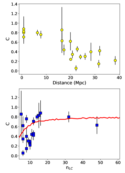
Figure 5: The dependence of recovery rate, C, of known variables on the distance of the host galaxy (upper panel) and on the average number of points in the light curve ($n_{\rm LC}$; lower panel) for galaxies in the Control Sample and in the Hoffmann et al. (2016) galaxy sample, observed with the ACS or the WFC3 instruments. The red line indicates the results of the simulations (see text).

6.2 Limitations

The users should be aware of the following limitations of the HCV catalog:

1. The HSC pipeline is designed to process the majority of ACS/WFC, WFC3/UVIS, WFC3/IR, and WFPC2 images. Its main design goal was applicability to a wide variety of input data, rather than extraction of all possible information from a given data set (which would require fine-tuning of the analysis procedure for these specific data). The HSC (and the HCV) pipeline design is a compromise between the general applicability and quality of the output.

2. The HSC is built from visit-combined images. This means that on one hand, it does not go as deep as a mosaic combining all visits of this specific field could go. On the other hand, the time resolution of the HSC is not a good as it could be, had the individual exposure images been used for photometry.

3. The synthetic error analysis is not capable of removing all the corrupted measurements. Thus, visual inspection of HLA images, light curves, and CMDs is highly recommended when using the HCV catalog, at least for the part of the catalog that has not been validated by the experts.

4. For extended objects, the aperture centering algorithm, which is used to determine MagAper2, does not always yield the same exact pixel for different images of filters. This may result in apparent variability due to the offset of the D-parameter. Also, the aperture sizes used for MagAper2 may be too small for the deep fields where false variability may be induced by the changes of the PSF (Villforth et al., 2010). This should be considered when studying deep fields, such as CANDELS, RELIC, CLASH, etc.

5. During the expert validation of the multi-filter variable candidates, some GroupIDs (or subgroups) were found to exhibit a relatively large fraction (in some cases over 10%) of variable candidates, whereas, normally, the fraction of variable candidates is around 2-3%. This is due to corrupted photometry caused by the reasons outlined in this section, or proper motion. For instance, in the “Sagittarius Window Eclipsing Extrasolar Planet Search” (SWEEPS) fields, a fraction of sources have been split into two MatchIDs because of the detection of their large proper motions, as the two major observation periods are separated by $\sim$3000 days. The large amount of false candidates in such fields significantly delays the process of validation, forcing us to not fully expert validate all the unreliable groups. We suggest that users are cautious when exploiting these groups. Here is a list of the 25 unreliable GroupIDs(_subgroups): 24555, 33004, 33109, 53275, 56019, 73455, 289829, 439774_5, 439774_8, 1024360, 1033498, 1033692, 1039945, 1040910, 1042327, 1043384_0, 1043756, 1045492, 1045904_8, 1045904_57, 1045904_102, 1045904_108, 1047823, 1063416, 1073046. It should be noted that version 3.1 of the HSC (released on 2019 June 26, after submission of this paper) provides proper motions for 400,000 sources in the SWEEPS field.

6. Some fields were found to contain a large number of outliers, which are mainly due to saturation and a diffuse background. In the case of saturation, it generally occurs in globular clusters in the Milky Way (e.g., NGC 6397) or nearby galaxies with long exposures (e.g., HIGH-GALACTIC-LATITUDE fields in the SMC), in which a small to large number of saturated stars create spikes and/or halos crossing the whole image and degrade the photometry. For cases with a diffuse background, which is typically related to star formation regions (e.g., 30 Doradus, Westerlund 2) or spiral galaxies with a large amount of gas and dust, the nebulous structures/clumps are sometimes detected by SExtractor  since it is designed to measure such extended objects.

7. The quality of photometry is degraded in fields containing large numbers of bright stars (Milky Way globular clusters like NGC 6397 and the fields in the SMC) which create diffraction spikes, halos, and saturation trails (due to charge bleeding) that together affect a large fraction of the image area.

8. In diffuse background regions with nebulosity (30 Doradus, Westerlund 2) or spiral galaxies, the nebulous clumps are sometimes detected as discrete objects and enter the HSC and our variability analysis.

9. Prior to HSC v3, we found that there was a general problem of image alignment both for the white-light and single-filter visit-combined images, which leads to outliers in the light curves and consequently false variables. Those misalignments are generally caused by a failure to reacquire the guide stars after an Earth occultation (affecting the white-light image), or a slight drift and/or (small) rotation between exposures (affecting the single-filter visit-combined image). We recommend a careful look at the color images to make sure the stars are circular. For the few fields with a large number of observations in different filters, the alignment between different filters and exposures is more difficult. Furthermore, there are cases of “intrinsic” misalignment, such as moving objects (e.g., nearby stars with high proper motions, planets). Since HLA DR10 is the first data release that fixes misalignment between both exposures and filters, HSC v3 data from both ACS and WFC3 should have very good alignment.

10. Besides the “physical misalignment” issue described above, an algorithm failure in the crossmatching of the same source between different filters/exposures also occurred occasionally during the construction of the HSC and resulted in outliers in the light curve and false variability in the HCV catalog. However, this is fairly rare and mostly occurs in crowded fields and/or IR wavelengths (e.g., NGC 4258).

11. The tremendous improvements in the image processing of the latest release of the HLA, and therefore in the photometry and astrometry of the HSC, are mainly available for ACS and WFC3 data, not for WFPC2 data. At the moment, the HSC data quality is relatively lower for WFPC2, making source detections from WFPC2 data in the HSC and variability detection in the HCV catalog less reliable. Furthermore, the data quality in the IR is relatively lower compared to the optical bands, that is for WFC3/IR versus the WFC3/UVIS, and ACS/WFC data, due to the more complicated instrumental effects (e.g., cosmic rays and snowballs, on-orbit degradation, image persistence, large background fluctuation, blobs, and optical anomalies).

12. The cadence of observations may affect the detection of variability. When several visits are taken in a relatively concentrated time period or relatively equal intervals, which can form a baseline for the preprocessing, the output of the HCV pipeline is reliable. However, if there is a big gap (e.g., several months or years) between two observational periods, the instrumental conditions and/or sky background subtraction may change and result in false variability. These effects are supposedly corrected by the preprocessing, but special attention is also needed when dealing with such cases, especially when there is only single observation after/before the gap.

13. Another problem of the HSC is that sometimes more than one measurements were kept in the database for the same source in a given image. This is likely due to that a source with critical size may appear slightly different in each image and just above the deblending threshold of SExtractor. Occasionally one source may be split into two, resulting in a double-detection for the same source. Although the cross-matching of HSC white-light sources between images is initially done by using a friends-of-friends (FoF) algorithm with a specified search radius and a Bayes factor, some of the double-detections are not identified and merged during the process. The HCV pipeline has excluded all targets with double-detections.

14. There are still some remaining issues in the data set which are poorly understood. One such issue is that some “variable candidates” exhibit step-shaped light curves with a rapid jump or drop, which can reach up to about one magnitude (e.g., NGC 1015, NGC 1448, NGC 2442, NGC 7250, M31-POS44, Leo A). Those targets are inevitably selected by the pipeline due to the large scatter in the light curves. Visual inspection indicates that some of them are extended gaseous structures or image artifacts, while others are real objects. The spatial distribution of those targets is also not fully in accordance with the CCD gaps. The exact cause of this phenomenon is currently under investigation. It may be due to the rotation of the telescope, which results in different CTE correction and background subtraction.

    Another issue is that in a few fields, some light curves show very similar tendencies or shapes (e.g., NGC 2070, NGC 6388), which may be related to uncorrected systematic effects. Again, this is inevitable due to the complicated observational strategies and instrumental conditions of HST. Moreover, for some fields, the saturation flag is not fully working (e.g., NGC 1851). For instance, one of the filters combined in the white-light image may be heavily saturated, which causes photometric degradation in other filters. For some deep fields (e.g., fields from RELICS, Hubble Frontier Fields), we also notice that an unusually large fraction of point sources show variability in their light curves and are selected as variable candidates, while the reason for this is still unknown. Crowding is generally an issue for globular clusters of the Milky Way, where the targets in the central region are largely blended, with corrupted photometry. Finally, due to HST observational strategies, the HSC also includes some measurements from single, long exposures, which are heavily contaminated by cosmic rays.

7 Results

The HCV processing pipeline identified 84,428 variable candidates by applying the detection and validation algorithm to the sources in the HSC v3 that passed the preprocessing procedure. Table 5 summarizes the results: out of 15,160 GroupIDs in the HSC v3, 250 GroupIDs met the selection criteria. Out of the 108 million sources (MatchIDs) in the HSC, 3.7 million sources passed the selection criteria and were processed by the DPP. This corresponds to 3.4% of the sources and 1.6% of the GroupIDs. The distribution of the number of sources per GroupID is illustrated in Figure 6. Histograms for the whole HSC v3 catalog and also for the HCV catalog are plotted. The cut-off at N${}_{\rm sources}\geq 300$ appears to be near the peak of the distribution of the number of sources in the HSC.

In total, 84,428 sources (i.e., 2.3% of the sources processed) were automatically flagged by the pipeline as variables, including 73,313 (87% of the total) single-filter and 11,115 (13% of the total) multi-filter variable candidates. The expert validation procedure was applied to 49% of the multi-filter (after excluding unreliable groups rejected by the experts, see Section 6.2) and 11% of the single-filter candidates, which corresponds to 16% of the total variable candidates. The results of the expert validation procedure are summarized in Table 6 and are indicative of the reliability of the automatic classification by the DPP. About 40% of the variables were classified as high-confidence variables, while on average 41% were classified as probable variables and 19% as possible artifacts. There is a higher incidence of possible artifacts (22%) among SFVCs than among MFVCs (16%), as expected. If we extrapolate to the whole HCV catalog, this implies that $81\%$ of the variable candidates are true variables, while the remaining $19\%$ are artifacts. It should be noted that among multi-filter variables, the success rate is even higher (84%). These percentages were derived excluding the unreliable groups that were rejected by the experts.

In Figure 7, we present the median time baseline (i.e., the time difference in days between the first and the last observation of a source) as a function of the median number of data points in the light curve ($n_{\rm LC}$) for all 250 GroupIDs processed by the DPP, color-coded by HST instrument. Clearly, WFC3 and ACS contribute more GroupIDs and therefore more variable candidates to the HCV catalog than WFPC2. The time baseline ranges from under a day to over 15 years with a relatively flat distribution among the GroupIDs and a peak between 200–2000 days. The number of data points in the HCV light curves ranges from five (our cut-off limit) to 120. A typical variable in the HCV catalog will have up to ten data points in its light curve. Given the relatively small number of points in the light curves, the HCV catalog does not provide classifications for the variable sources.

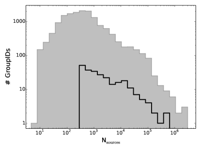
Figure 6: Histogram of the number of sources vs. number of GroupIDs for the entire HSC v3 (gray) and the HCV catalog (black).

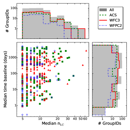
Figure 7: The median time baseline as a function of the median number of data points for all 250 GroupIDs processed by the HCV pipeline, labeled by HST instrument: ACS (green squares), WFC3 (red triangles), and WFPC2 (blue asterisks). The side plots present histograms of the median time baseline and number of data points in light curves, respectively. The histogram lines are color-coded as above, while the gray shaded histogram denotes the total distribution of the three instruments.

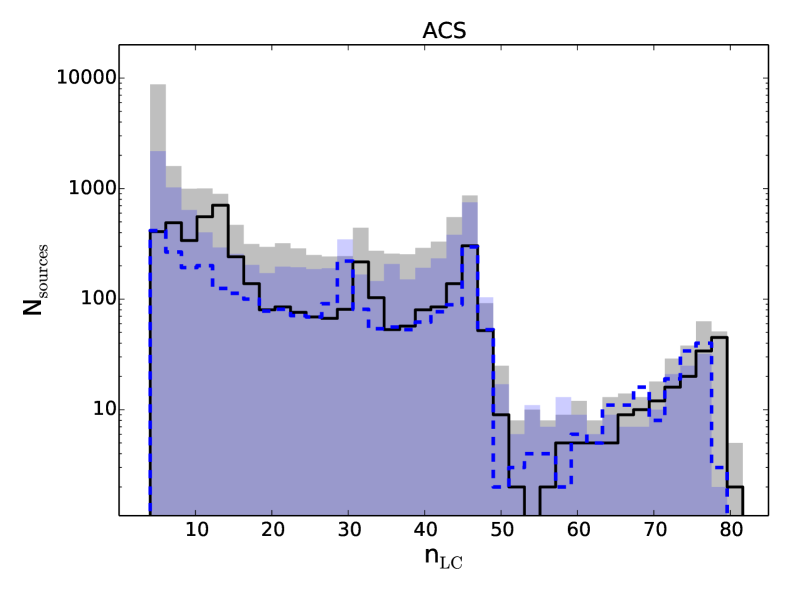
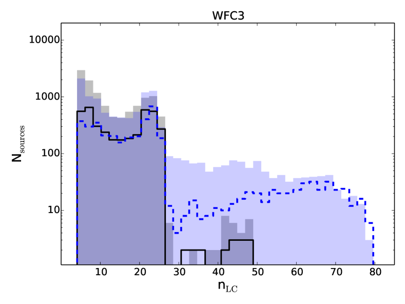
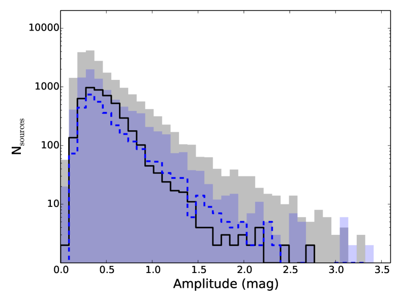
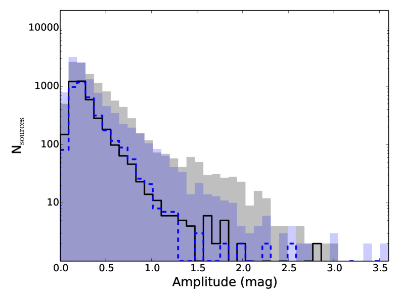
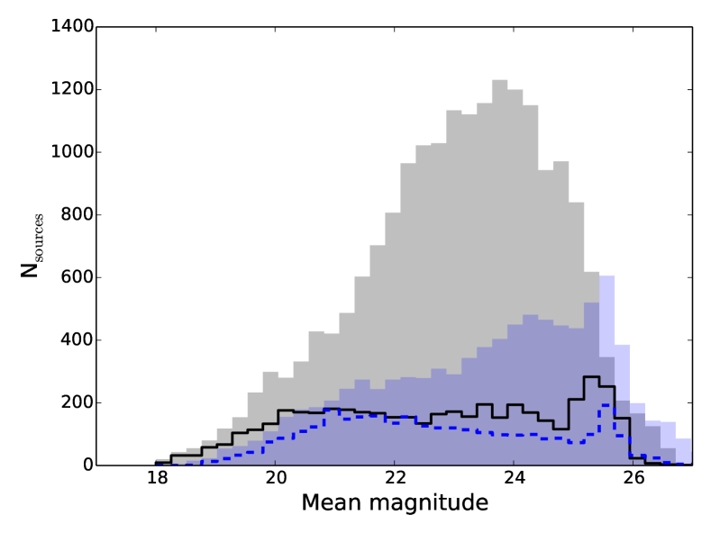
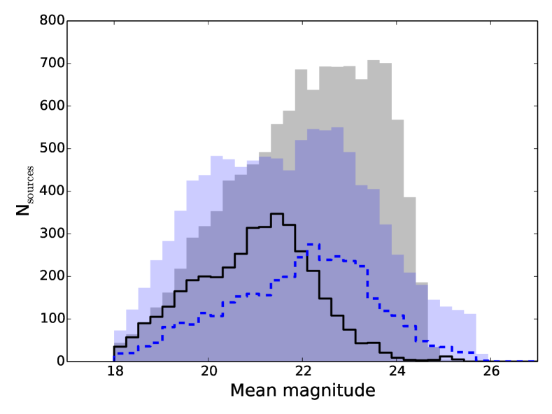
Figure 8: Histogram of the number of data points in a light curve, $n_{\rm LC}$ (upper panel), the amplitude of variability (middle panel) and mean magnitudes (lower panel), for all multi-filter (lines) and single-filter (filled histograms) variable candidates detected by the HCV pipeline in the F814W and F606W filters of ACS (left) and WFC3 (right). In F814W (F606W), the SFVCs are shown with a gray (blue) histogram, while the MFVCs with a solid black (dashed blue) line.

The HCV catalog includes 47 instrument and filter combinations, of which the ACS_F814W (with 19,550 SFVC and 4,762 MFVC detections in this filter), ACS_F606W (with 8,807 SFVC and 3,017 MFVC detections in this filter), WFC3_F814W (with 11,356 SFVC and 3,935 MFVC detections in this filter), and WFC3_F606W (with 10,457 SFVC and 3,702 MFVC detections in this filter) contain the largest number of candidate variables. In Figure 8 we present histograms of the number of data points per light curve ($n_{\rm LC}$), the amplitude of variability and the mean magnitudes of the variables for the four most commonly used instrument and filter combinations. The multi-filter and single-filter variable candidates are plotted separately. The distribution of $n_{\rm LC}$ shows several peaks, with the maximum $n_{\rm LC}$ for ACS in the histogram bin with values 12.5–15 for the MFVCs and 5–7.5 for the SFVCs. There is a steep drop for sources with $n_{\rm LC}>45$. For WFC3, the SFVCs peak at 5–7.5, while the MFVCs have a second peak at $\sim$20–25. There is a steep drop at values $n_{\rm LC}>27$ for the MFVCs, while the drop is more gradual for the SFVCs. The middle panel shows the distribution of the amplitude, with a peak in the distribution in the bin with values $0.2-0.4$ mag. We note the large number of variables with amplitudes $>1$ mag (see Section 7.4). The lower panel shows the distribution of the mean magnitude of each variable light curve. For ACS, the SFVCs are distributed as expected, increasing in numbers toward fainter magnitudes and dropping after a peak around magnitude 24, where the completeness drops. However, the MFVCs peak around magnitude 25.5, due to the large number of RR Lyrae and Cepheids detected with ACS in nearby galaxies (e.g. Hoffmann et al., 2016), which appear at these magnitudes. Another factor contributing to the almost flat distribution is the fact that both RR Lyrae and Cepheids have a larger amplitude in the blue than in the red, so they often do not appear as MFVCs. In WFC3, the distributions resemble those of a magnitude limited sample, except for the SFVCs in F606W, which display a secondary peak around magnitude 23.

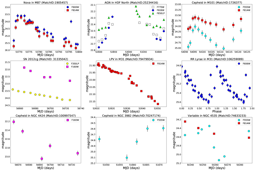
Figure 9: Example light curves for different types of variable sources in the HCV catalog. From left to right and top to bottom, we show the light curves of a classical nova in M87, an AGN in HDF North, a classical Cepheid in M101, SN 2012cg in NGC 4424, an LPV in M31, a RR Lyrae in M31 (phased with P=0.688 days), two Cepheids in NGC 4424 and NGC 3982 with sparse light curves, and a variable in NGC 4535. Error bars are plotted, although they are sometimes smaller than the symbol size. The variables in the first six panels were observed with the ACS instrument, while the variables in the three lower panels were observed with WFPC2.

We demonstrate the light curve quality and types of variability included in the HCV catalog in Figure 9, which presents five multi-filter variables: a classical nova, an AGN, a classical Cepheid, a supernova, and a variable in NGC 4535, as well as four single-filter variables: a long period variable (LPV), a RR Lyrae star, and two classical Cepheids with sparse light curves. The AGN has not been previously reported as a variable. It should be noted that despite the preprocessing applied by the pipeline, outliers do remain, for example, in the nova and RR Lyrae curves (see Section 6).

Table 5: Results of the HCV data processing pipeline.

Item	Number
GroupIDs in HSC v3	15,160
GroupIDs (subgroups) processed by DPP	250 (2,132)
GroupIDs with variable candidates	244
GroupIDs with single-filter variable candidates	243
GroupIDs with multi-filter variable candidates	127
Sources processed by DPP	3,679,859
Variable candidates found by DPP	84,428
Single-filter variable candidates	73,313
Multi-filter variable candidates	11,115

Table 6: Results of the expert validation for SFVCs and MFVCs. Percentages for the expert validated variables are computed relative to the number of variables in the HCV catalog, while percentages in the following columns are computed relative to the number of expert validated variables.

Type of variable	# HCV catalog	# expert validated	# high-confidence	# probable	# possible
candidate	variables	variables	variables	variables	artifacts
Single-filter	73,313	8,139 (11%)	3,323 (41%)	3,055 (37%)	1,761 (22%)
Multi-filter	11,115	5,394 (49%)	2,101 (39%)	2,442 (45%)	851 (16%)
Sum	84,428	13,533 (16%)	5,424 (40%)	5,497 (41%)	2,612 (19%)

7.1 The catalog release

The catalog is available in its entirety via the ESA Hubble Science Archive (eHST; Arévalo et al., 2017) and the HCV Explorer at ESAC. Moreover, the catalog can be queried via the MAST interface at STScI. The HCV Explorer is a web visualization tool that will allow the user to access and explore the Hubble Catalog of Variables. The first release of the tool will offer interactive and connected plotting of the variables in the HCV catalog in a region of the sky. By selecting a variable from the finder chart, one can display and download its light curve, view the location of the source on a MAD vs. magnitude diagram, and download the light curve for this source, as well as for non-variable sources in the same GroupID or subgroup. The visualization of the results will help the user to assess whether a candidate variable is reliable or not, particularly in cases where no expert validation has been performed. This paper includes the following release tables: an overview table of the distribution of variables per GroupID (Table LABEL:hcv_tableMFVCs), the catalog of variables (Table 10), and the catalog of sources that fall below the 5$\sigma$ MAD detection threshold for variability selection, meaning the “constant” stars (Table 11).

While a total of 250 GroupIDs were processed by the DPP, there are only 244 GroupIDs with a multi-filter and/or single-filter variable candidate detection. The six GroupIDs without detected variables are: 1423, 4006, 29216, 31829, 1024871, and 1042864. The multi-filter variable candidates are detected in 127 GroupIDs, while the single-filter variable candidates in 243 GroupIDs (see also Table 5). Out of the 244 GroupIDs with variables, 21 GroupIDs (25 subgroups) were flagged as unreliable by the experts (see Section 6) and therefore the variables included in these GroupIDs were not expert validated. Table LABEL:hcv_tableMFVCs presents the 244 GroupIDs with detected variables. It lists the coordinates, field name (from the HLA), the initial number of sources that passed to the DPP (to which prior selection criteria were applied), the final number of sources (from which the variable candidate sources were searched for detection), the maximum number of instrument and filter combinations available per GroupID, and the number of multi-filter and single-filter variables in each GroupID. It is ordered by right ascension. The field name “ANY” and names containing “PAR” refer to observations obtained in parallel to the main science target.

Table 10 is the HCV catalog release. The sources listed correspond to ten entries of the catalog, while the columns show, for each source: the equatorial coordinates, the MatchID, the GroupID, the subgroup, the pipeline classification flag, the expert-validation classification flag, the number of existing instrument and filter combinations for the source, the name of the instrument and filter combination for which the following data are given: the filter detection flag, which indicates whether the variable was detected [“1”] or was not detected [“0”], the variability quality flag, the number of measurements in the light curve $n_{\rm LC}$, the HSC magnitude m${}_{\textrm{HSC}}$ (i.e., the mean MagAper2 of the light curve points), the corrected magnitude m${}_{\textrm{HCV}}$, the MAD value, and the reduced $\chi^{2}$ value. For all MFVCs, there are extra columns for each additional instrument and filter combination, in which the source is classified as a variable candidate (provided in the online version of the catalog).

Table 11 presents the sources that fall below the 5$\sigma$ detection threshold, which include constant sources and possibly, low-amplitude variables below our detection threshold. The sources listed correspond to the first ten entries of the catalog, while the columns show, for each source: the equatorial coordinates, the MatchID, the GroupID, the subgroup, the number of instrument and filter combinations in which individual sources are observed, the name of the instrument and filter combination for which the following data are given: the number of measurements in the light curve $n_{\rm LC}$, the HSC magnitude m${}_{\textrm{HSC}}$, the corrected magnitude m${}_{\textrm{HCV}}$, the MAD value, and the reduced $\chi^{2}$ value. A block of information, identical to columns (7) to (12), is added for each additional instrument and filter combination, in which the source has been observed (provided in the online version of the catalog).

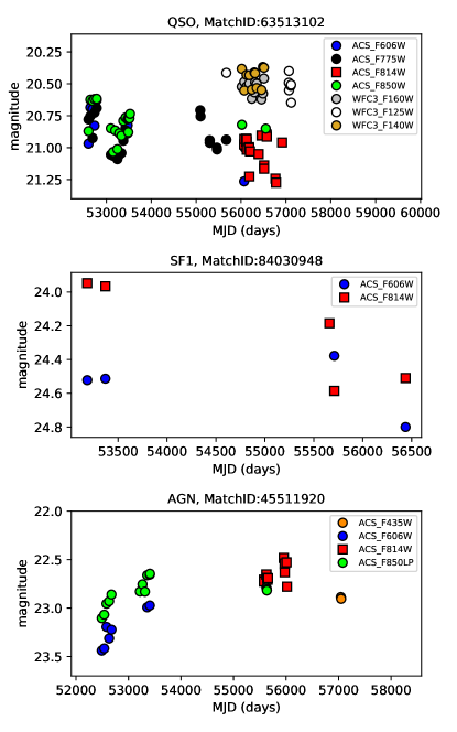
Figure 10: Examples of three variable sources in the CANDELS fields: a quasar in GOODS-North (upper panel), a Seyfert-1 in GOODS-South (middle panel), and a new variable AGN in EGS (lower panel).

7.2 Comparison of HCV catalog variables with SIMBAD

In order to estimate the fraction of new variables included in the HCV catalog, we cross-matched the high-confidence (expert-validated) variables with SIMBAD using a conservative search radius of 5”, to account for possible errors in the astrometry of published variables. This yielded a total of 2,839 matches out of 5,424 high-confidence variables, implying that 2,585 (48%) are potentially new variables, as they have no matches in SIMBAD. A careful cross-match with other bibliographical data is necessary to assess whether these sources are indeed newly detected variables. It is also interesting to note that the most common SIMBAD classes for the matched objects were Cepheids and RR Lyrae variables, while several other classes of variables were identified such as eclipsing binaries, long-period variables, novae, supernovae, AGN, etc. Even among the 2,839 matched objects there are several cases where the SIMBAD classification does not indicate variability (e.g., “star”). Some of these may be mismatches, due to the large search radius. Therefore, there may be several new variables in the sample of “matched” objects as well. Projecting these results to the entire HCV catalog, we expect a few thousand new variables.

7.3 Variable AGN in the HCV catalog

Variability is a basic characteristic of AGN at all wavelengths, appearing over periods of hours to years (Ulrich et al., 1997). Optical variability has therefore been used as a method to identify AGN (Pouliasis et al., 2019; Sarajedini et al., 2011; Villforth et al., 2010, 2012; De Cicco et al., 2015; Falocco et al., 2016); the importance of the method is demonstrated by its ability to identify low-luminosity AGN that even the deepest (currently available) X-ray observations would have missed. The HCV catalog contains many groups with deep observations obtained over multiple visits, making them appropriate for identifying variable AGN (spanning the range from the most luminous point-like quasars to the low-luminosity AGN). Here, we demonstrate the power of the HCV catalog in the “Cosmic Assembly Near-IR Deep Extragalactic Legacy Survey” fields (CANDELS; Koekemoer et al., 2011; Grogin et al., 2011). The HCV catalog contains 621 variable candidates (179 MFVCs and 442 SFVCs) in the five CANDELS fields (GOODS South, GOODS North, COSMOS, EGS, and UDS). Following the expert validation of the sources, we excluded the sources classified as “possible artifacts”, resulting in 171 variable candidates.

We cross-matched our variable sources with the SIMBAD database (using a radius of 1”) to validate their nature. Table 7 presents the results for the different fields. Excluding the stellar population, 75% and $\sim$45% of the “high-confidence” and “probable” variable sources, respectively, are confirmed AGN or quasars. Regarding the rest of the sources showing variability, but which are classified as ’normal’ galaxies in SIMBAD and do not show any X-ray emission, the aforementioned studies have shown that these extended sources are consistent with low-luminosity AGN (LLAGN), which would have been missed by the current depths of X-ray surveys, but are important to complete the AGN demographics. In Figure 10, we present three example light curves of variable sources in the CANDELS fields that are classified via spectroscopy as AGN or quasars. MatchID=45511920 is reported to be variable for the first time. We thus demonstrate the photometric quality of extended sources and, in particular, variable AGN in the HCV catalog.

Table 7: HCV variables in the CANDELS fields.

Item	GOODS-N	GOODS-S	COSMOS	EGS	UDS	Total
	1084534	1084533	1081922	1045196	1036556
Pipeline class. MFVCs/SFVCs	75/143 (218)	90/164 (254)	2/52 (54)	10/50 (60)	2/33 (35)	179/442 (621)
Expert validated MFVCs/SFVCs	58/- (58)	28/17 (45)	2/- (2)	6/31 (37)	-/28 (28)	95/76 (171)
AGN / Seyfert 1 / Seyfert 2	11	13	-	16	-	40
Quasars	11	10	-	3	2	26
Stars	19	10	1	-	-	30
Normal galaxies (LLAGN)	18	10	1	6	13	48
Total classified sources (SIMBAD)	59	43	2	25	15	144

7.4 High-amplitude variables or transients in the HCV catalog

The HCV catalog contains a large number of high-amplitude variables / transients. The number of variable candidates in the HCV catalog with amplitudes $\geq 1$ mag in at least one filter is around 6,500 (Spetsieri et al., in prep.). We have selected three high-amplitude, multi-filter sources that were serendipitously discovered during the expert validation procedure to present below. These sources have not been previously reported in the literature. Light curves and finder charts of these three multi-filter variables are presented in Figure 11 and are described below.

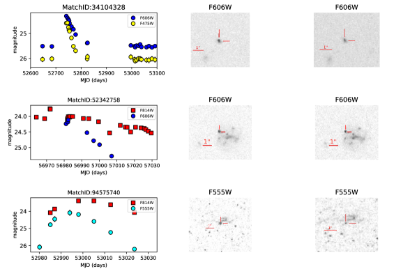
Figure 11: HCV catalog light curves and finder charts of the newly-discovered high-amplitude, multi-filter variables in the fields of NGC 3314 (first row), MACSJ1149.5+2223-HFFPAR (second row), and NGC 4258 (third row). The finder charts on the left correspond to the light curve peak, while those on the right to the minimum.

1. Transient object in the field of NGC 3314: This source has a MatchID=34104328 in the HSC v3 and is located at R.A.: 10:37:15.601 and Dec.: $-$27:40:03.42 (J2000). The HCV light curve of the source contains 24 observations in filters F475W and F606W of ACS (see Figure 11). The object reaches a peak magnitude of 24.32 mag in F606W and 24.5 mag in F475W at MJD=2452741.2064 days and fades by 1 mag in F606W and 1.5 mag in F475W in about 80 days. The F475W$-$F606W color of the host galaxy is 0.5 mag. The nature of this transient is difficult to determine, as there is no redshift information or any estimate of the intrinsic luminosity. However, we excluded the possibility of it being a Tidal Disruption Event (TDE), since TDEs show no color evolution, while this object evolves to the red. Also, the rise and fall timescales exclude the possibility of the object being a Type Ia SN. If we assume that it is associated with NGC 3314 (e.g., a low-mass, low-surface brightness satellite galaxy in the field), the absolute magnitude of this object would be $\sim-12$ mag, which is typical for novae. However, the shape of the light curve resembles a core-collapse SN. We performed fits using SALT2-extended (Guy et al., 2007; Pierel et al., 2018) and Nugent templates (Gilliland et al., 1999). SN IIn templates (based on blackbody templates from Di Carlo et al., 2002) yielded the best fit at z$\sim$1.2. SN IIP templates also provided a good fit, while SN IIL templates a poor fit. Hence, based on the photometric classification, we suggest that this object is a candidate high-redshift, core-collapse SN IIn or SN IIP, which is not associated with NGC 3314.

2. Variable in MACSJ1149.5+2223-HFFPAR:

   This source has a MatchID=52342758 in the HSC v3 and is located at R.A.: 11:49:36.684 $\&$ Dec.: +22:17:14.37 (J2000) in the MACSJ1149.5 parallel field, near a faint galaxy. The HCV light curve of this source is shown in the second panel of Figure 11 and contains seven data points in the F606W and 25 in the F814W filter, obtained with ACS. As shown in Figure 11 the light curve peaks around magnitude 24 at MJD$\simeq$56972.0934 days in F814W. In F606W the peak is followed by a steep, linear decline of $\sim$1.2 mag within 20 days after the peak, whereas the light curve in F814W drops by $\sim$ 0.8 mag. Unfortunately, there are gaps in the coverage in both filters. We attempted to fit SN templates, which indicate that it might be a high-redshift superluminous SN. The date of maximum according to the fit occurs at MJD=56984.679 days.

3. SN Ia in the field of NGC 4258:

   This source has a MatchID=94575740 in the HSC v3 and is located at R.A.: 12:19:25.639 and Dec.: +47:10:30.52 (J2000) in the field of NGC 4258. The HCV light curve includes 12 data points in F555W and six data points in F814W, spanning about 40 days. The light curve shows the early evolution of a possible SN; the peak brightness is followed by a decrease of $\sim$2 mag in F555W and $\sim$1 mag in F814W within 20 days. SALT2-extended provided a good fit for a SN Type Ia, with a maximum at MJD=53000.022 days.

8 Summary

We present the Hubble Catalog of Variables, a new catalog of variable sources based on photometry from the Hubble Source Catalog version 3, which includes all available images obtained with WFPC2, ACS, and WFC3 onboard the Hubble Space Telescope that were public as of October 2017. The HCV catalog is the first catalog of variables from the HST. It contains 84,428 variable candidates with $V\leq 27$ mag, which were identified among sources having at least five measurements in the same instrument and filter combination, in groups having at least 300 sources. The HCV catalog is the deepest catalog of variables available, reaching on average $\sim 4$ mag deeper than current catalogs of variable sources.

The HCV system, developed from scratch for this project, comprises of a data processing pipeline, catalog, and bridge to the science archives at ESAC. The architecture, main elements of the pipeline, implementation technologies, and performance are presented. In brief, we developed a preprocessing algorithm for identifying and removing outlier measurements. We further applied a local zeropoint correction. We used ten “Control Sample” fields to evaluate all intermediate steps and refine our selection criteria and thresholds. A total of 250 GroupIDs (or 2,132 subgroups) including 3.7 million sources finally satisfied our selection criteria and were processed through the pipeline.

The data processing pipeline calculated the median absolute deviation and used a 5$\sigma$ threshold to select variable candidates. These were passed to the validation algorithm, which classified the sources as single or multi-filter variable candidates and assigned a variability quality flag to each source. The pipeline identified 84,428 variable sources: 73,313 single-filter and 11,115 multi-filter variable candidates. The data points in the HCV catalog light curves range from five to 120, the time baseline ranges from under a day to over 15 years, while $\sim$8% of variables have amplitudes in excess of 1 mag. Furthermore, expert validation was performed on 16% of the total number of variables. The result of this procedure implies that about 80% of the sources are true variables, while about 20% may be possible artifacts. It should be noted that classifications of the variable sources are not provided. We finally summarize the challenges present in identifying variables in a large and inhomogeneous set of photometric measurements, which are specific to Hubble.

We expect the HCV catalog to become a key resource for the community, as it includes variable stars in the Milky Way and nearby galaxies, as well as transients, and variable AGN, which include low-luminosity AGN. Possible uses include searches for new variable objects of a particular type for population analysis, detection of unique objects worthy of follow-up studies, identification of sources observed at other wavelengths, and photometric characterization of candidate progenitors of SNe and other transients in nearby galaxies. The HCV catalog contains many interesting high-amplitude variables, including a core-collapse SN and a Type Ia SN reported here for the first time. A thorough analysis of the high-amplitude variables in the HCV catalog will be presented by Spetsieri et al. (in prep.).

The catalog is available via eHST at ESAC and MAST at STScI. Both platforms allow for the visualization of the results. In principle, the HCV pipeline can be used to generate future versions of the catalog based on future HSC releases.

Appendix A Comparison of variability indices with HSC-based simulations

Before selecting MAD as our primary variability detection statistic (Sec. 4) we investigated the performance of 18 variability indices using diverse sets of ground-based photometric data (Sokolovsky et al. 2017b). We also explored the possibilities to enhance the variability detection efficiency by combining multiple indices via the principal component analysis (Moretti et al. 2018) and machine learning (Pashchenko et al. 2018). While combining multiple indices did show promise, the diverse nature of the HSC data (and the resulting difficulty of constructing the training data set) together with the difficulty of implementing the machine learning techniques under our data processing architecture (Java and Apache Spark; Sec. 2.2; that had to be chosen early in the project) lead us to favor the simple approach of using one general-purpose index for variability detection.

We follow the procedure for the simulations described in Sec. 3.8 of Sokolovsky et al. (2017b) to identify the index that is best suited for finding variable objects in the HSC data. The index should be sensitive to various types of variability and tolerate the wide range of observing cadence patterns found in the HSC, as well as occasional outlier measurements caused by cosmic ray hits and calibration errors. The cosmic rays are a major problem for space-based photometry as illustrated by the light curve in Fig. 12. These observations consist of a single 20 s exposure in the F775W filter per HST visit, that is the exposures were not split into cosmic ray pairs (Sec. 1.1) making this data set heavily contaminated by cosmic rays, despite the short exposure time. The outlier points in Fig. 12 are all caused by cosmic ray hits, as can be seen from inspecting the corresponding images (Fig. 15). Observations split into multiple exposures are less affected by cosmic rays (Sec. 1.1), however the probability of two cosmic rays hitting the same pixel in two images is non-negligible, and the edges of the stacked frame may be covered by only one image if dithering was applied.

To preserve the sampling and noise properties of the HSC data in our simulations we use the HSC light curves of sources from selected control sample fields (Enoch et al. 2012, describe the use of non-variable object light curves as a realistic photometric noise model). We exclude the sources known to be variable and inject 1% of the non-variable sources with artificial variability. The variability is modeled as a simple sine variation with an amplitude randomly selected for each model variable source to be between 0 and 1 mag (c.f. the experimental amplitude distribution presented in Fig. 8), the frequency of variations between 0.05 and 20.0 cycles/day (periods in the range 0.05 to 20.0 days; the model distribution is uniform in frequency, so it has more short-period variables compared to a uniform distribution in period). The initial phase of the sine variation is also chosen randomly for each object. Having the list of objects in which we injected artificial variability, we perform magnitude-dependent thresholding for each of the tested variability indices. For each index we test a range of thresholds between 0 and $50\sigma$ and adopt the threshold that provides the highest efficiency in recovering the artificial variables. Changing the threshold is needed to account for the fact that some variability indices have a non-gaussian distribution of their values for non-variable sources. Different thresholds may be optimal for different variability indices.

The efficiency of variable source selection is quantified with the $F_{1}$ score (Rijsbergen 1974) which is the harmonic mean of the precision and recall. It reaches the maximum value of 1.0 when all the variable sources are recovered above the threshold while all the non-variable sources are below the threshold. We refer to the maximum $F_{1}$ score obtained over the trial thresholds as $F_{\rm 1\,max}$. The following indices were tested: reduced $\chi^{2}$ ($\chi_{\rm red}^{2}$) weighted standard deviation ($\sigma_{w}$), median absolute deviation (${\rm MAD}$), interquartile range (${\rm IQR}$), robust median statistic (${\rm RoMS}$), normalized excess variance ($\sigma_{\rm NXS}^{2}$), peak to peak amplitude $v_{\rm peak-to-peak}$, lag-1 autocorrelation $l_{1}$, Welch-Stetson variability index ($I$), Stetson’s $J$ index and its variations ($J({\rm time})$, $J({\rm clip})$, $L$), consecutive same-sign deviations from the mean magnitude (${\rm CSSD}$), excursions ($E_{x}$), inverse von Neumann ratio ($1/\eta$), excess Abbe value ($\mathcal{E}_{\mathcal{A}}$), and $S_{B}$ statistic. The references to the previous uses of these indices to characterize photometric variability may be found in Table 8. The definitions of these indices may be found in Sokolovsky et al. (2017b) while Pashchenko et al. (2018) discuss correlations between the indices (the degree of correlation depends on the data). The VaST code (Sokolovsky & Lebedev 2018) was used to perform the simulations.

The simulation results for six data sets from the Control Sample are presented in Table 8. The reported $F_{\rm 1\,max}$ are the median values over 100 implementations of the procedure of injecting random amplitude/period/phase/ sine variability into a random set of light curves within the data set. The data sets were obtained with different cameras, cover a different time range (Table 4), and differ in the number of observations (the median number of light curve points, $n_{\rm LC}$, is reported in Table 8). One important difference between the observations of M4 in F467M and F775W filters is that the latter were taken with only one 20 sec exposure per visit and are therefore have more cosmic ray contamination (resulting in more photometric outliers) than the former (five 392 sec exposures per visit). This results in a dramatic difference in $F_{\rm 1\,max}$ values for the variability indices that are not robust to outliers (such as $\sigma_{w}$), while the robust indices (like $MAD$ and $IQR$) remain efficient (retain their high $F_{\rm 1\,max}$ scores). This is also evident from comparing Fig. 12 and Fig. 14 discussed below.

The fact that the indices that characterize light curve smoothness (Table 8) are not performing as well as the robust measures of scatter is a feature of the simulation: we injected variability with timescales that, in most cases, are shorter than the observing cadence, and therefore, the resulting light curves are not going to be smooth. This relation between the variability timescale and the observing cadence is expected to be common in the HCV catalog as many of the time-series HST observations are optimized for long-period (high-luminosity) Cepheids, while RR Lyrae stars and eclipsing binaries that may be present in the same data tend to vary on shorter timescales.

In order to simulate how the variability detection efficiency changes with the number of points in the light curve we repeat the above simulations for the WFC3 F775W and F467M filter observations of M4, randomly selecting only $n_{\rm LC}$ observations from this data set and removing all others. The procedure is repeated 1000 times for each value of $n_{\rm LC}$ and the resulting median $F_{\rm 1\,max}$ scores (for three variability indices quantifying scatter) are reported in Fig. 13 and Fig. 14. The F775W data set is heavily contaminated with cosmic rays, which results in a poor performance of $\sigma_{w}$ compared to the robust indices MAD and IQR. In the presence of outliers, for the small number of points $4<n_{\rm LC}<10$ MAD provides noticeably higher $F_{\rm 1\,max}$ values compared to IQR, however, the opposite is true for the F467M data set where outliers are a negligible problem (see also NGC 4535 simulations in Table 8). The simulation results support the expected trend: as long as there are no outlier measurements, non-robust measures of scatter ($\sigma_{w}$) should be more accurate than the robust ones for a given number of points, while in the presence of outliers we expect the opposite. The fact that for the F467M simulations (Fig. 14) MAD and IQR outperform $\sigma_{w}$ for $n_{\rm LC}\gtrsim 20$ suggests that this data set is not completely free of outliers, they are just considerably less common than in the F775W data set. In the regime $4<n_{\rm LC}<10$, where the difference between the two robust indices, IQR and MAD is evident (Fig. 13 and Fig. 14), the $F_{\rm 1\,max}$ score of the IQR (which can tolerate a smaller percentage of outliers compared to MAD) lies between MAD and $\sigma_{w}$, providing a compromise between robustness and sensitivity.

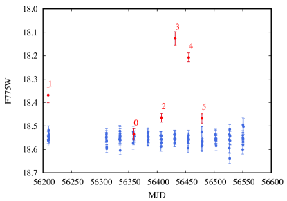
Figure 12: Light curve of HSC v3 source with MatchID=45740877 from the field of the globular cluster M4 (GroupID=33675) observed with WFC3. The numbered red points correspond to measurements obtained from the images presented in Fig. 15.

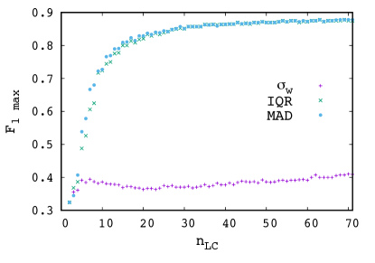
Figure 13: Variability detection efficiency ($F_{\rm 1\,max}$ score) as a function of the number of points in the light curve. The simulated variability was injected into the WFC3_F775W filter observations of M4. The data set is heavily affected by cosmic rays, resulting in the poor performance of $\sigma_{w}$ compared to the robust indices MAD and IQR.

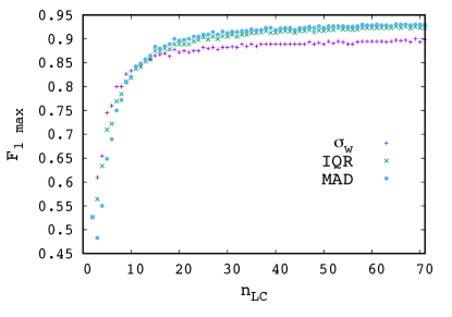
Figure 14: Variability detection efficiency ($F_{\rm 1\,max}$ score) as a function of the number of points in the light curve. The simulated variability was injected into the WFC3_F467M filter observations of M4. Unlike the F775W data (Fig. 13), the F467M data are not heavily affected by cosmic rays. Under such conditions, $\sigma_{w}$ performs better than the robust indices MAD and IQR for light curves having a small number of points.

Table 8: Comparison of $F_{\rm 1\,max}$ values for the tested variability indices.

Field	M4	M4	M31-Halo11	M31-Halo11	NGC 4535	NGC 4535
Instrument	WFC3	WFC3	ACS	ACS	WFPC2	WFPC2
Filter	F467M	F775W	F814W	F606W	F555W	F814W
$n_{\rm LC}$	82	55	32	28	9	7
Indices characterizing light curve scatter
$\chi_{\rm red}^{2}$	0.87	0.31	0.86	0.83	0.33	0.27
$\sigma_{w}$	0.89	0.47	0.87	0.84	0.55	0.39
${\rm MAD}$	0.93	0.90	0.89	0.86	0.57	0.40
${\rm IQR}$	0.92	0.90	0.89	0.86	0.67	0.50
${\rm RoMS}$	0.91	0.86	0.89	0.85	0.43	0.35
$\sigma_{\rm NXS}^{2}$	0.07	0.07	0.02	0.02	0.09	0.06
$v_{\rm peak-to-peak}$	0.81	0.09	0.72	0.75	0.38	0.31
Indices characterizing light curve smoothness
$l_{1}$	0.20	0.16	0.03	0.03	0.04	0.03
$I$	0.56	0.48	0.40	0.36	0.02	0.02
$J$	0.59	0.59	0.81	0.76	0.44	0.33
$J({\rm time})$	0.55	0.50	0.40	0.36	0.21	0.15
$J({\rm clip})$	0.89	0.81	0.82	0.79	0.44	0.33
$L$	0.59	0.63	0.82	0.77	0.46	0.40
${\rm CSSD}$	0.02	0.02	0.02	0.02	0.02	0.02
$E_{x}$	0.55	0.17	0.69	0.68	0.32	0.33
$1/\eta$	0.17	0.14	0.03	0.02	0.04	0.03
$\mathcal{E}_{\mathcal{A}}$	0.02	0.02	0.02	0.02	0.03	0.02
$S_{B}$	0.73	0.48	0.74	0.68	0.24	0.22

References: $\chi_{\rm red}^{2}$ (de Diego 2010), $\sigma_{w}$ (Kolesnikova et al. 2008), ${\rm MAD}$ (Zhang et al. 2016), ${\rm IQR}$ (Sokolovsky et al. 2017b), ${\rm RoMS}$ (Rose & Hintz 2007), $\sigma_{\rm NXS}^{2}$ (Nandra et al. 1997), $v_{\rm peak-to-peak}$ (Brown et al. 1989), $l_{1}$ (Kim et al. 2011), $I$ (Welch & Stetson 1993), $J$ (Stetson 1996), $J({\rm time})$ (Fruth et al. 2012), $J({\rm clip})$ (Sokolovsky et al. 2017b), $L$ (Stetson 1996), ${\rm CSSD}$ (Shin et al. 2009), $E_{x}$ (Parks et al. 2014), $1/\eta$ (Shin et al. 2009), $\mathcal{E}_{\mathcal{A}}$ (Mowlavi 2014), $S_{B}$ (Figuera Jaimes et al. 2013).

Appendix B Additional tables

Table 9: HCV multi-filter and single-filter variable candidates per GroupID.

R.A. (J2000)	Dec. (J2000)	GroupID	Field Name	# Initial	# Final	# Filters	# MFVC	# SFVC
(degrees)	(degrees)			sources	sources
0.495079472	-15.511714610	1062949	WLM-STARCLUS	35990	31117	4	121	236
3.475747041	-30.390185660	1042688	ABELL-2744-HFFPAR	1732	1495	7	13	11
3.576352357	-30.398039800	1043761	AC118	2466	1688	7	23	39
3.894313004	-32.187015950	66669	ESO410-005	17988	9633	1	0	19
5.065006551	59.308725250	92609	IC10-POS2	102640	44822	1	0	967
5.660203860	-72.068720590	439774	NGC104-WFC-UPDATE	254025	77634	18	93	2026
5.965410502	-24.709494760	66514	SCL-DE1	3732	1813	1	0	7
6.544826341	-11.079992920	1037352	CETUS-DWARF	5342	4026	2	52	111
6.636002643	-41.857497960	66572	ESO294-010	14545	7093	1	0	19
8.199983458	48.378008730	1033762	NGC147	36417	27339	2	32	186
8.284913184	48.290157600	1010724	ANY	3298	2424	2	0	13
8.873996052	36.503287960	1045103	ANDROMEDA-III	6614	5381	2	21	105
8.954952633	-43.206258020	1074873	SPARCS-J003550-431210-COPY	711	519	2	7	1
9.799728109	48.435035430	1033573	NGC185	28758	21130	2	138	341
9.932522332	48.415645960	1012451	ANY	4056	3034	2	7	88
10.134718080	40.746713140	1078908	M31-B005	10432	1242	1	0	45
10.942091470	41.001298780	1045904	M31	11525935	551781	5	107	6386
10.958906840	39.770107650	1033697	ANY	1739	1376	2	0	17
11.017427590	-20.564792110	1064963	XMM44	625	443	2	3	8
11.082702210	39.784454780	1033421	M31-TIDALSTREAM1	8957	6792	2	12	20
11.296398110	-73.211160770	56019	HIGH-GALACTIC-LATITUDE	68231	49329	3	491	1641
11.315025630	38.004159700	1071126	ANY	1368	1122	2	2	23
11.428953570	38.042769870	1064398	ANDROMEDA-I	14801	12576	2	92	151
11.526879280	40.698480400	1043756	M31-B379	14359	11509	2	34	57
11.575856070	-73.342660500	1060093	SMC-F18-WFC	87220	313	2	0	2
11.639456390	40.671999130	1043755	ANY	2073	1751	2	9	28
11.658976770	-73.176846010	289829	LIST-1	6708	3740	3	1	80
12.270891940	40.301782090	439858	NGC224-22KPC	2026	1402	2	0	4
12.288275700	42.759679010	1033359	M31-OUTERDISK1	13974	10644	2	12	59
12.404305260	42.707136260	1033692	ANY	2291	1884	2	7	31
13.370965580	39.832611450	445976	NGC224-35KPCA	1456	1179	2	1	11
13.537404890	39.797394510	439608	NGC224-35KPCB	1333	1082	2	0	14
13.641544760	-72.648447860	1044880	HIGH-GALACTIC-LATITUDE	65347	3872	1	0	73
13.805802780	-72.507935970	289947	LIST-1	5902	828	3	3	32
13.904171110	-72.407267470	408245	LIST-1	3231	549	1	0	13
14.614070700	-72.249865720	353029	LIST-1	5771	2526	3	19	116
14.780237720	-72.188553230	1053537	NGC346	46234	7918	2	10	134
14.879852610	32.393442050	1045492	ANDROMEDA-XVI	1743	940	2	4	11
15.958660810	21.882082220	1063351	PISCES-I	5233	3826	2	17	58
16.046030500	2.220925169	1045442	IC-1613-FIELD2	475	370	1	0	11
16.120357510	2.156895687	69810	IC1613	27045	23106	2	97	167
17.376581170	35.725221740	36624	NGC404	1884	862	1	0	9
17.447468470	-72.875866490	87786	HIGH-GALACTIC-LATITUDE	20894	11501	1	0	187
17.516163190	-2.414328481	1011552	HI-LAT	991	408	3	0	3
17.768124330	-72.891846220	55509	HIGH-GALACTIC-LATITUDE	20675	15780	1	0	82
17.939753130	-35.062271290	1049880	CLH12-WFC3POINTING	1310	898	1	0	5
18.575030230	38.119420470	1045180	ANDROMEDA-XV	2460	1599	2	9	69
19.021788990	33.365106150	1058861	ANY	1088	838	2	9	20
19.098526490	33.434377400	1042143	ANDROMEDA-II	12018	9470	2	72	166
23.490565100	30.407033710	1062832	M33	1060282	51548	4	2	562
24.205936780	41.524189800	87237	UNKNOWN-TARGET-1	590	352	1	0	2
28.178193340	-13.945233640	23565	GAL-CLUS-015245-135737-POS08	1179	390	2	0	4
31.442579700	-58.483479470	1039295	SPT0205-E08-418-MIDPOINT	756	617	2	13	8
32.432429460	-4.614702546	46172	SGR-STREAM-1	1440	531	1	0	8
34.357051550	-5.204224549	1036556	Z7-GIANTLAE	11352	3966	4	2	33
35.280507730	35.941622150	64702	QSO-022105+355613	1074	653	1	0	1
35.716451440	42.488242950	1037724	SN1986J	3113	1729	1	0	13
36.111153410	-3.391831535	1061394	SPARCSJ0224	598	435	2	3	3
36.780796660	33.590610420	538286	NGC925	2132	1261	1	0	14
39.539658600	-1.329463556	1028931	N1015	5380	3611	2	0	53
39.971081180	-1.586147087	1033838	SNABELL370	3265	2053	7	45	73
40.045881850	-34.543154630	1059852	FORNAX-CLUSTER4	8757	3371	3	23	58
40.058950060	-1.616596037	1083558	ABELL-370-HFFPAR	1700	1455	7	11	14
42.112940520	-3.540953533	1021022	CALIGULA3	732	319	1	0	1
48.413834080	-67.193566610	1079516	ANY	555	339	3	2	7
50.521822860	-15.395683500	24452	SN-2012Z	11519	8637	3	19	181
51.276873770	-36.358279700	483765	NGC1326A	730	498	2	1	6
52.727948060	-28.722348560	1054528	SPARCSJ0330	606	445	2	3	3
53.177857170	-27.922753570	1084533	UDF$\_$(Merged)	25224	14278	9	90	164
53.403340700	-36.128855350	331331	SN2001DU	9046	571	1	0	7
55.553912440	-29.899653340	483481	NGC1425	661	388	1	0	8
56.092058410	-43.534428460	1075853	ERIDANUS2	4005	2106	1	0	10
56.102155050	-44.599903700	1045280	SN2003HN	13312	9228	2	1	145
64.037020340	-24.072588440	1042781	SN-M0416-IR	2552	1830	7	33	49
64.105624000	-24.137125440	1040153	MACSJ0416.1-2403-HFFPAR	1865	1404	7	13	10
64.392534960	-62.782648480	1084480	SN-2009IB	32051	18461	1	0	269
70.360306470	-2.871318803	360365	SN1999EM	1556	1054	2	1	21
77.375965220	-69.129122470	1048097	NGC-1856	36678	11914	1	0	173
78.517988600	-40.054597500	33004	NGC1851	28212	17926	2	13	546
80.484860210	-69.502344530	1056946	OGLE052218.07-692827.4	172529	89657	1	0	585
84.114945230	-70.116525640	381717	LIST-1	4372	1114	3	10	43
84.245627080	-66.363422320	1042179	STAR-CLUS-053707-662203	2939	1588	1	0	16
84.479026430	-69.245704330	1039945	STAR-0537-6910	580832	195362	27	468	4062
86.752544600	-34.281952750	177255	NGC2090	1281	881	2	0	18
86.978237130	-70.230020860	56487	HIGH-GALACTIC-LATITUDE	38162	25934	1	0	512
106.021557800	-3.845185765	1034275	V838-MON-ECHO-COPY	1435	811	2	1	37
109.395422800	37.760470440	62353	MACSJ0717.5+3745-POS5	6078	3622	7	109	117
110.830281800	-73.463489250	1073046	SMACSJ0723.3-7327	683	369	2	5	24
114.119408100	-69.554788310	73455	SN1999GA	25654	17433	2	4	246
114.609685100	65.464465330	25090	NGC2403-HALO-2	2124	1192	2	1	21
116.219973700	39.467756870	72495	MACSJ0744.9+3927-Y1	1027	395	2	7	6
122.229472100	6.728621118	81871	GRB021211	1088	357	1	0	1
123.659412000	49.056726260	483544	NGC2541	1018	584	1	0	12
138.027065000	-64.864488840	33470	NGC2808Y98B	75279	30350	3	85	1336
138.272575500	-64.844977390	25262	NGC-2808	4424	2970	2	5	96
140.524832700	50.953679330	18944	SN1999BY-3	1366	755	1	0	15
143.481802700	55.240553530	36988	IZW18-MAINBODY	1542	1106	3	1	18
143.656096600	17.125358980	1028455	LEO-T	526	381	1	0	2
143.728037200	17.047714070	1042327	LEO-T	5444	3693	2	13	12
147.753382800	33.559296090	24555	NGC3021-ACS	3287	2345	2	2	38
148.803039200	69.690576730	74633	M82	21706	15801	2	4	71
149.856321900	30.750169960	1037445	LEOA-CENTER	24301	19744	2	79	308
150.040369000	2.473513981	1081922	cosmos	20657	6331	4	2	52
152.089378700	12.300086950	25044	LEO-I-DSPH	71454	37739	1	0	135
153.522443000	0.642359289	1049163	MOO1014-E08-470	806	643	2	7	4
154.970955500	45.622203040	1038808	NGC3198	1236	699	1	0	14
155.450557800	18.092720520	1046053	LEOP	2110	1438	2	7	17
156.021671300	-57.762214380	1054696	WESTERLUND2	10687	5011	1	0	362
159.292264000	-27.662112840	38905	NGC3314-UPLEFT	4106	3260	2	14	108
159.799993500	41.681218920	483536	NGC3319	988	589	1	0	12
160.978310200	11.694576450	1030272	SN2012AW	2206	885	1	0	23
161.324267200	-60.020004420	22917	Eta-Car	50270	14325	3	0	550
161.610152900	-59.609894150	55731	ANY	5007	3322	1	0	66
161.777281200	11.827124280	1080182	SN1998BU-3	666	314	1	0	11
161.781170900	17.287822220	92880	NGC3370-ACS	10033	7518	2	10	59
161.933161600	13.988115580	27681	NGC3377-NUC1	10270	1735	1	0	13
162.053871700	12.602878380	1041148	NGC3384-POS-W	27966	8732	2	7	182
162.296210500	-53.329749320	1083958	LUHMAN16ABMINAPNE1	1038	784	2	0	14
162.342403100	56.678447920	1047807	SPARCSJ1049-REPOINT	482	329	2	3	2
163.351519900	16.775237110	1028736	N3447	9128	6964	2	0	58
168.421973200	22.201180510	1014062	LEOII-Q111340+221242	2593	1129	2	7	35
169.587190100	-32.780711850	1031228	NGC3621-OFF	1836	1019	1	0	22
170.083899500	12.983679220	445382	SN2009HD	3553	637	1	0	8
173.222913500	-76.017929400	91445	ANY	907	411	1	0	3
175.692407600	15.456023330	1080745	MOO1142	632	444	2	3	5
177.387087900	22.398492700	66095	REFSDALREAPPEARANCE	6130	3877	9	42	63
178.930006300	55.322777590	1083372	NGC3972	8085	5492	2	3	143
179.126633000	55.125475070	73298	NGC4051	736	350	1	0	4
180.485472500	-18.883810650	1043713	NGC4038-S-TAIL	1595	422	1	0	12
182.648904000	39.403874870	1017300	NGC4151	13752	5789	1	0	59
184.838133500	47.391646000	1043384	UGC-07356	114212	61491	8	230	830
185.791870500	15.804409580	47524	SN2006X	2721	868	1	0	23
186.599851500	31.221500200	499217	SN2013DF	804	461	1	0	16
186.797143900	9.462037454	1045340	SN2012CG	11400	6814	2	1	46
186.804972300	23.858403990	1046067	COMA-BERENICES-V22	5680	1062	2	0	5
187.048255300	12.560581790	1934	VIRGO-ICFIELD3	1456	1201	2	0	9
187.168581400	62.637148600	1084534	HDF$\_$(Merged)	23045	13837	10	75	143
187.468856200	7.981483036	1040498	VCC1226	1837	820	4	0	5
187.713602300	12.390529780	1072340	M87	26817	15731	4	31	157
187.914199500	3.928083565	1051133	SDSS-588010877688807475	1943	1233	1	0	27
188.484162300	2.608183274	508907	NGC4527	930	371	1	0	2
188.569682600	8.165917216	209749	NGC4535	1537	1032	2	5	21
188.594096100	2.143856732	1079995	NGC4536-WFPC2	1279	767	1	0	6
188.867305200	14.469535620	531865	NGC4548	1343	968	2	0	15
189.018156800	26.033051320	46574	NGC4565-HALO3	31651	1848	2	5	26
189.233096200	14.214497220	529814	NGC4571	1119	691	1	0	10
189.955780500	-11.441077530	1074339	ANY	4640	407	1	0	4
190.220145100	-40.965968070	531716	SN2008CN	1162	639	1	0	21
190.724637900	13.255459210	1009478	NGC4639	1071	624	1	0	8
190.917643000	11.594597720	1038219	VCC1978-OFFSET	1773	684	2	0	11
192.659387700	25.546854610	555853	NGC4725	704	393	1	0	7
194.286273300	34.321497660	1076197	CVNII-Q125704+341920	2433	1278	1	0	7
195.354923200	27.884096870	74366	NGC4921-PA299	4387	2812	2	0	21
195.480154400	27.881910250	1039468	ANY	1671	325	3	0	14
197.871282200	-1.346418497	1033313	ABELL1689-POS3	2005	1442	2	0	10
198.205971300	-47.475380210	45491	ER8-FIELD	1486	434	1	0	12
201.375683100	-42.981138010	1055708	SN2016ADJ	2159	375	1	0	7
201.379131000	-47.577621440	1080307	WCEN	57830	26673	9	40	744
201.781488400	-47.499462370	12611	OMEGACEN-3	246460	166087	13	879	6685
201.969708500	-31.506322180	21359	ESO444-G046	6035	2124	1	0	8
203.817517400	40.995825340	1077193	ACO-1763	728	417	2	3	13
206.886618400	-11.754619380	23539	RXJ1347.5-1145	628	383	3	15	12
209.276881100	4.515200147	35730	REF13	903	321	3	1	0
210.817624000	54.159625820	1053852	M101-A	280111	136077	9	669	1803
211.208077800	54.472818010	1043478	M101-NE-PLUME3	4276	2643	2	1	30
211.991244600	-11.411374500	37745	FIELD-140801-1126H	6822	5242	1	0	11
215.110454900	52.971386610	1045196	SN1997A2	19733	5749	5	10	50
215.588734400	-0.399217810	1013227	NGC5584	16211	13660	3	32	105
215.950589100	24.090980410	62371	ROSE-GRISM	757	432	3	4	4
216.447362500	35.543002490	82373	FIELD-142549+353248	611	311	1	0	1
216.633965900	35.151219170	1030110	ISCS25.687	802	488	2	12	2
218.111565900	32.827098630	1034184	ISCSJ1432.4+3250	623	471	2	7	3
218.649094600	59.333769890	1028696	U9391	3003	2341	2	0	21
227.458545100	67.295365940	1052878	URSA-MINOR-GALAXY-4-COPY-1	9771	671	2	4	24
229.640406500	2.080274917	33584	M5	61211	18872	3	63	940
230.375962800	-7.386011459	1027929	SN2005CF	3464	2075	2	1	72
244.159754000	-22.920672690	1039049	M-80	952	476	2	0	3
244.258760500	-22.978397670	33079	M80-WFPC2	20832	12857	4	4	299
245.896921400	-26.526456380	33675	M4-CORE	11299	8460	2	10	120
245.984119900	-26.533600770	304489	M4-4-CORE-RADII	711	493	2	7	19
246.445580100	-72.202364880	65764	NGC6101	5451	3249	3	1	68
247.825014800	-40.323817340	516320	LOW	1378	843	1	0	40
247.891084800	37.613912910	1009308	PAR	694	376	4	1	6
248.131039900	-13.042828370	33308	NGC6171-M107	3760	1278	1	0	48
250.793840200	39.339911080	1030681	ANY	452	322	1	0	1
259.276716700	43.138331520	33610	NGC6341-POS1	48146	11185	1	0	336
264.070239500	-44.725694360	33109	NGC6388	78750	38240	3	53	316
265.157698900	-53.681256880	33688	NGC6397-HH	19462	10711	5	9	306
265.266884700	-53.741198200	1033498	NGC6397-WFPC2	48150	32139	2	117	1309
265.627413000	-40.260208250	1030256	LOW	4723	778	1	0	65
266.356899900	-29.030646960	88697	SGRA-NC	89152	6695	1	0	260
267.147272100	-20.312820830	1046062	ANY	45958	26078	2	4	288
267.227849200	-20.375595770	1024360	PSR6440B	86322	67371	3	404	2328
267.602621300	-37.131468260	1033918	NGC-6441-OFF	39823	16139	1	0	168
268.128047600	-17.688308660	521507	SAKURAI-NOVALIKE-VAR	3541	2922	2	28	117
269.020511000	-21.955747840	63563	LOW	5820	2577	1	0	103
269.676660500	-29.142625410	1063416	WFPC2-2	394202	277258	2	1098	5961
269.817975500	-29.194997840	1040910	SWEEPS-R1	689565	548735	2	2374	13683
269.833593400	-29.271668850	1061725	ANY	171177	132584	2	810	2981
269.842928000	-29.327223720	1047823	ANY	170242	134197	2	835	2997
271.836126900	-24.999712230	17120	NGC6544	26359	14421	2	18	292
274.687931600	-13.747139180	1045014	M16-A	3345	468	1	0	19
275.923454300	-30.360921720	68312	NGC6624-WFPC2-POS4	2932	1181	1	0	1
280.733373100	-32.220545050	1039204	PAR	2748	409	1	0	7
280.801687700	-32.294429130	33390	NGC6681-WFPC2-POS4	2583	1040	1	0	1
280.960699300	-32.334952990	423081	ANY	2035	960	1	0	29
283.767304900	-30.271751110	510437	SGR-DSPH2	3186	399	1	0	11
283.801435200	-31.346838320	507380	ANY	1522	781	1	0	19
284.066234000	-37.853507310	519756	LOW	588	423	1	0	25
286.980282200	-18.768425360	525031	LIST-1	804	540	2	8	37
287.722874300	-59.974237780	33701	PSR-J1911-5958A	53907	25691	5	44	870
290.212620800	37.800541050	1008520	NGC6791	2778	1381	2	0	14
291.088415100	9.895533570	1063228	VY2-2-COPY	6343	2187	4	1	23
292.296639300	-6.869730730	93958	ANY	2616	1728	1	0	31
292.501623500	-17.669640940	22844	SAGITTARIUS-DWARF-IRREGULAR	13602	7671	1	0	195
292.853101400	-26.536974030	1024716	MACS1931-WFC3PAR1	835	378	2	2	30
292.982474000	11.036191290	381893	ANY	2324	476	1	0	30
295.659026100	-10.329599350	1014035	NGC6814	7331	5757	2	3	32
296.659407700	-19.605604900	82136	GRB020813	1441	351	1	0	1
299.679758600	35.247485890	420853	ANY	1437	572	1	0	27
299.838458900	40.852085320	509388	PARALLEL-FIELD	709	385	1	0	10
303.791751800	6.210771995	1024567	GRB120923A	596	389	1	0	3
308.811011400	60.195994110	1037524	SPIRITS-15AFP	20341	5989	1	0	80
310.249431200	-44.860242880	1044811	SPT2040	868	708	2	13	14
311.715749600	-12.835157210	1041481	DDO210	11216	9450	2	75	92
316.524228400	-58.749529310	1039240	SPT-CLJ2106-5844	831	675	2	15	10
322.337010400	0.172586888	1040914	RXJ2129-WFC3PAR2	1029	667	2	0	17
322.364992000	-7.681219071	62377	MACSJ2129-0741	792	399	2	8	12
322.427334200	12.222673330	353549	ANY	3800	2576	1	0	139
322.579603100	12.115746100	25292	M15-SECOND	6044	1958	1	0	106
325.094528200	-23.185945480	33571	NGC7099-WFPC2-POS4	6480	779	1	0	3
325.150647700	-23.236204030	514176	NGC7099-OUTER	1247	639	1	0	21
334.366518600	0.134914196	19330	TARGET6	3510	953	2	0	6
334.423026200	0.834759540	19400	SA22POINTL36	1241	763	5	5	13
334.585476300	40.550329410	1027220	SN2013DY	4741	2921	2	0	93
338.175007100	31.211115750	1045157	ANDROMEDA-XXVIII	4028	3078	2	17	56
338.247644200	-60.546434810	79757	HDFS	789	420	2	0	26
339.266996300	34.468875420	555871	NGC7331-POS1	996	641	1	0	27
340.450104200	-64.420934510	1037453	TUCANA-DWARF	6210	4838	2	69	234
342.170209300	-44.530294380	1042675	RXJ2248-ROT	2751	1768	7	44	44
342.318216500	-44.548460310	1075304	RXJ2248-WFC3PAR2	1723	1434	7	17	17
350.777554300	58.787328770	53275	CAS-A-WEST	5091	560	3	13	27
352.062055100	14.780585490	1051244	ANY	2880	2574	2	0	29
352.156042200	14.724993450	1064674	PEGASUS-B	55108	45352	2	228	747

Table 9: continued.

Table 10: The HCV catalog.

R.A. (J2000)	Dec. (J2000)	MatchID	GroupID	Subgroupa	Pipeline	Expert	# Filters	Filter	FilterDetection	VarQuality	nLC	¡mHSC¿	¡mHCV¿	MAD	$\chi_{\rm red}^{2}$
(degrees)	(degrees)				Class.b	Class.c			Flagd	Flage		(mag)	(mag)
0.4281922281	-15.4549541473	51033165	1062949	-5	1	0	2	WFC3_F814W	1	- - - - -	12	24.165	24.166	0.043	4.4
0.4620466232	-15.5108289719	17833555	1062949	-5	1	0	2	ACS_F814W	1	CAAAB	12	24.897	24.897	0.023	3.7
0.4634322822	-15.5074214935	44149982	1062949	-5	2	1	2	ACS_F814W	1	AABAA	11	25.713	25.713	0.148	29.4
0.4645933211	-15.5040855408	44006736	1062949	-5	1	0	2	ACS_F814W	1	AAAAB	12	26.013	26.013	0.177	7.1
0.4657302499	-15.5397748947	104466632	1062949	-5	1	0	1	ACS_F814W	1	AAAAC	6	24.642	24.642	0.063	5.0
0.4685320258	-15.5385761261	49380750	1062949	-5	1	0	2	ACS_F814W	1	AAAAC	10	23.449	23.448	0.035	38.5
0.4685845673	-15.5160827637	41579373	1062949	-5	1	0	2	ACS_F814W	1	BAAAB	11	24.528	24.527	0.021	1.2
0.4689802527	-15.5137805939	86716251	1062949	-5	1	0	2	ACS_F814W	1	AAABB	12	23.734	23.733	0.020	15.7
0.4693635106	-15.5307703018	105204801	1062949	-5	2	1	2	ACS_F814W	1	BABAB	10	25.750	25.750	0.177	14.7
0.4695036709	-15.5268716812	12663862	1062949	-5	1	0	2	ACS_F814W	1	AAAAC	12	21.971	21.971	0.026	104.1

Table 11: Catalog of sources that were not classified as variable candidates by the HCV pipeline.

R.A.	Dec.	MatchID	GroupID	Subgroupa	# Filters	Filter	nLC	¡m${}_{\textrm{HSC}}$¿	¡m${}_{\textrm{HCV}}$¿	MAD	$\chi_{\rm red}^{2}$
(J2000)	(J2000)							(mag)	(mag)
0.3962652087	-15.4694614410	38868203	1062949	-5	2	WFC3_F475W	12	26.224	26.224	0.050	0.2
0.3999678493	-15.4831781387	41866145	1062949	-5	2	WFC3_F475W	12	25.431	25.431	0.027	0.1
0.4000068605	-15.4822616577	30810204	1062949	-5	1	WFC3_F475W	9	26.158	26.158	0.051	0.3
0.4021478295	-15.4797763824	95901547	1062949	-5	2	WFC3_F475W	12	25.889	25.889	0.024	0.1
0.4022069871	-15.4806766510	100130418	1062949	-5	2	WFC3_F475W	12	26.216	26.214	0.046	0.2
0.4026675820	-15.4820632935	37320200	1062949	-5	2	WFC3_F475W	12	26.001	26.000	0.033	0.2
0.4029722214	-15.4806251526	42893121	1062949	-5	2	WFC3_F475W	11	25.806	25.806	0.083	2.5
0.4030649364	-15.4813785553	46076923	1062949	-5	1	WFC3_F814W	10	25.499	25.499	0.015	0.2
0.4032958448	-15.4865312576	37088064	1062949	-5	1	WFC3_F814W	10	25.144	25.144	0.023	0.2
0.4034545422	-15.4482450485	77175405	1062949	-5	2	WFC3_F475W	11	26.233	26.233	0.021	0.0