Finite-size Scaling of O($n$) Systems at the Upper Critical Dimensionality

Abstract

Logarithmic finite-size scaling of the O($n$) universality class at the upper critical dimensionality ($d_{c}=4$) has a fundamental role in statistical and condensed-matter physics and important applications in various experimental systems. Here, we address this long-standing problem in the context of the $n$-vector model ($n=1,2,3$) on periodic four-dimensional hypercubic lattices. We establish an explicit scaling form for the free energy density, which simultaneously consists of a scaling term for the Gaussian fixed point and another term with multiplicative logarithmic corrections. In particular, we conjecture that the critical two-point correlation $g(r,L)$, with $L$ the linear size, exhibits a two-length behavior: following the behavior $r^{2-d_{c}}$ governed by Gaussian fixed point at shorter distance and entering a plateau at larger distance whose height decays as $L^{-d_{c}/2}({\rm ln}L)^{\hat{p}}$ with $\hat{p}=1/2$ a logarithmic correction exponent. Using extensive Monte Carlo simulations, we provide complementary evidence for the predictions through the finite-size scaling of observables including the two-point correlation, the magnetic fluctuations at zero and non-zero Fourier modes, and the Binder cumulant. Our work sheds light on the formulation of logarithmic finite-size scaling and has practical applications in experimental systems.

I Introduction

The O($n$) model of interacting vector spins is a much-applied model in condensed-matter physics and one of the most significant classes of lattice models in equilibrium statistical mechanics Fernández et al. (2013); Svistunov et al. (2015). The Hamiltonian of the O($n$) vector model is written as

$$\mathcal{H}=-\sum\limits_{\langle{\bf r}{\bf r^{\prime}}\rangle}\vec{S}_{\bf r}\cdot\vec{S}_{\bf r^{\prime}},$$ (1)

where $\vec{S}_{\bf r}$ is an $n$-component isotropic spin with unit length and the summation runs over nearest neighbors. Prominent examples include the Ising ($n\!=\!1$), XY ($n\!=\!2$) and Heisenberg ($n\!=\!3$) models of ferromagnetism, as well as the self-avoiding random walk ($n\!\rightarrow\!0$) in polymer physics. Its experimental realization is now available for various $n$ values in magnetic materials Merchant et al. (2014); Qin et al. (2015); Lohöfer and Wessel (2017); Qin et al. (2017); Cui et al. (2019), superconducting arrays Resnick et al. (1981); Goldman (2013) and ultracold atomic systems Greiner et al. (2002); Capogrosso-Sansone et al. (2007).

Finite-size scaling (FSS) is an extensively utilized method for studying systems of continuous phase transitions Cardy (2012), including the O$(n)$ vector model (1). Near criticality, these systems are characterized by a diverging correlation length $\xi\propto t^{-\nu}$, where parameter $t$ measures the deviation from the critical point and $\nu$ is a critical exponent. For a finite box with linear size $L$, the standard FSS hypothesis assumes that $\xi$ is bounded by the linear size $L$, and thus predicts that the singular part $f(t,h)$ of free energy density scales as

$$\begin{split}f(t,h)=&L^{-d}\tilde{f}(tL^{y_{t}},hL^{y_{h}})\end{split}$$ (2)

where $\tilde{f}$ is a universal scaling function, $t$ and $h$ represent the thermal and magnetic scaling fields, and $y_{t}=1/\nu$ and $y_{h}$ are the corresponding thermal and magnetic renormalization exponents, respectively. Further, the standard FSS theory hypothesizes that at criticality, the spin-spin correlation function $g(r,L)\equiv\langle\vec{S}_{0}\cdot\vec{S}_{\bf r}\rangle$ of distance $r$ decays as

$$g(r,L)\asymp r^{-(d-2+\eta)}\tilde{g}(r/L)\;,$$ (3)

where $\eta$ relates to $y_{h}$ by the scaling relation $\eta\!=\!2+d-2y_{h}$. From (2) and (3), the FSS of various macroscopic physical quantities can be obtained. For instance, from the second derivative of $f(t,h)$ with respect to $t$ or $h$, it is derived that at criticality, the specific heat behaves as $C\!\asymp\!L^{2y_{t}-d}$ and the magnetic susceptibility diverges as $\chi\!\asymp\!L^{2y_{h}-d}$. The FSS of $\chi$ can also be calculated by summing $g(r,L)$ over the system. Further, the thermodynamic critical exponents can be obtained by the (hyper-)scaling relations. For instance, in the thermodynamic limit ($L\rightarrow\infty$), the specific heat and the magnetic susceptibility scale as $C\propto t^{-\alpha}$ and $\chi\propto t^{-\gamma}$, where the critical exponents are $\alpha=2-d/y_{t}$ and $\gamma\!=\!(2y_{h}-d)/y_{t}$.

The O($n$) model exhibits an upper critical dimensionality $d_{c}\!=\!4$ such that the thermodynamic scaling in higher dimensions $d\!>\!d_{c}$ are governed by the Gaussian fixed point, which has the critical exponents $\alpha=0$ and $\gamma=1$ etc. In the framework of renormalization group, the renormalization exponents near the Gaussian fixed point are

$$y_{t}=2\hskip 14.22636pt\mbox{and}\hskip 14.22636pty_{h}=1+d/2$$ (4)

for $d>d_{c}$.

Accordingly, the standard FSS formulae (2) and (3) predict that the critical susceptibility diverges as $\chi\!\asymp\!L^{2y_{h}-d}\!=\!L^{2}$ for $d>d_{c}$. However, for the Ising model on 5d periodic hypercubes, $\chi$ was numerically observed to scale as $L\asymp L^{5/2}$ instead of $L^{2}$ Luijten (1997); Luijten et al. (1999); Wittmann and Young (2014); Kenna and Berche (2014); Flores-Sola et al. (2016); Grimm et al. (2017). The FSS for $d\geq d_{c}$ turns out to be surprisingly subtle and remains a topic of extensive controversy Luijten (1997); Luijten et al. (1999); Papathanakos (2006); Wittmann and Young (2014); Kenna and Berche (2014); Flores-Sola et al. (2016); Grimm et al. (2017); Zhou et al. (2018); Fang et al. (2019).

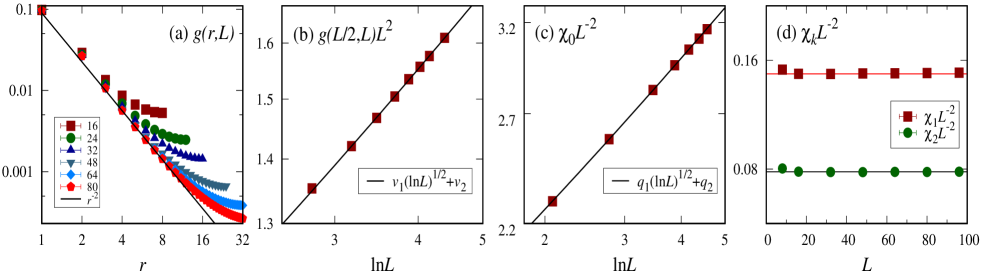
Figure 1: Evidence for conjectured formulae (11) and (12) in the example of the critical 4d XY model. (a) correlation function $g(r,L)$ in a log-log scale. The solid line stands for the $r^{-2}$ behavior. (b) scaled correlation $g(r,L)L^{2}$ with $r\!=\!L/2$ versus ${\rm ln}L$ in a log-log scale. Thus, the horizontal axis is effectively in a double logarithmic scale of $L$. The solid line represents logarithmic divergence with $\hat{p}\!=\!1/2$. (c) scaled magnetic susceptibility $\chi_{0}L^{-2}$ versus ${\rm ln}L$ in a log-log scale. The solid line accounts for logarithmic divergence with $\hat{p}\!=\!1/2$. (d) scaled ${\mathbf{k}}\neq 0$ magnetic fluctuations $\chi_{1}L^{-2}$ and $\chi_{2}L^{-2}$, with ${\mathbf{k}}_{1}\!=\!(2\pi/L,0,0,0)$ and ${\mathbf{k}}_{2}\!=\!(2\pi/L,2\pi/L,0,0)$, respectively. The horizontal lines strongly indicate the absence of logarithmic corrections in the scaling of $\chi_{\bf k}$.

It was realized that for $d>d_{c}$, the Gaussian exponents $y_{t}$ and $y_{h}$ in (4) can be renormalized by the leading irrelevant thermal field with exponent $y_{u}=4-d$ as Fisher (1971); Binder et al. (1985); Berche et al. (2012); Kenna and Berche (2013)

$$y_{t}^{*}=y_{t}-\frac{y_{u}}{2}=\frac{d}{2}\hskip 5.69054pt\mbox{and}\hskip 5.69054pty_{h}^{*}=y_{h}-\frac{y_{u}}{4}=\frac{3d}{4}\;,$$ (5)

and the FSS of the free energy density $f(t,h)$ becomes

$$\begin{split}f(t,h)=&L^{-d}\tilde{f}(tL^{y_{t}^{*}},hL^{y_{h}^{*}}).\end{split}$$ (6)

In this scenario of dangerously irrelevant field, the FSS of the critical susceptibility becomes $\chi\!\asymp\!L^{2y_{h}^{*}-d}\!=\!L^{d/2}$, consistent with the numerical results Luijten (1997); Luijten et al. (1999); Wittmann and Young (2014); Flores-Sola et al. (2016); Grimm et al. (2017). It was further assumed that the scaling behavior of $g(r,L)$ is modified as Kenna and Berche (2014)

$$g(r,L)\asymp r^{-(d-2+\eta_{Q})}\tilde{g}(r/L)$$ (7)

with $\eta_{Q}=2-d/2$, such that the decay of $g(r,L)$ is no longer Gaussian-like. In the study of the 5d Ising model Luijten (1997), a more subtle scenario was proposed that $g(r,L)$ decays as $r^{-3}$ at short distance, gradually becomes $r^{-5/2}$ for large distance and has a crossover behavior in between. The introduction of $\eta_{Q}$ was refuted by Wittmann and Young (2014) as the magnetic fluctuations at non-zero Fourier mode ${\bf k}\!\neq\!0$ scale as $\chi_{\bf k}\asymp L^{2}$ and underlined in Flores-Sola et al. (2016) which revealed that the non-zero Fourier moments are governed by the Gaussian fixed point instead of being contaminated by the dangerously irrelevant field.

Using random-current and random-path representations Aizenman (1982, 1985, 1986), Papathanakos conjectured that the scaling behavior of $g(r,L)$ has a two-length form as Papathanakos (2006)

$$g(r,L)\asymp\begin{cases}r^{-(d-2)},&r\leq\mathcal{O}\left(L^{d/[2(d-2)]}\right)\\ L^{-d/2},&r\geq\mathcal{O}\left(L^{d/[2(d-2)]}\right)\;.\end{cases}$$ (8)

According to (8), the critical correlation function still decays as Gaussian-like, $g(r,L)\asymp r^{-(d-2)}$, up to a length scale $\xi_{1}=L^{d/[2(d-2)]}$, and then enters an $r$-independent plateau whose height vanishes as $L^{-d/2}$. Since the length $\xi_{1}$ is vanishingly small compared to the linear size, $\xi_{1}/L\rightarrow 0$, the plateau effectively dominates the scaling behavior of $g(r,L)$ and the FSS of $\chi$. The two-length scaling form (8) has been numerically confirmed for the 5d Ising model and self-avoiding random walk, with a geometric explanation based on the introduction of unwrapped length on torus Grimm et al. (2017). It is also consistent with the rigorous calculations for the so-called random-length random-walk model Zhou et al. (2018). It is noteworthy that the two-length scaling is able to explain both the FSS $\chi_{0}\equiv\chi\asymp L^{5/2}$ for the susceptibility (the magnetic fluctuations at zero Fourier mode) Luijten et al. (1999) and the FSS $\chi_{\bf k}\asymp L^{2}$ for the magnetic fluctuations at non-zero modes Wittmann and Young (2014); Flores-Sola et al. (2016).

Combining all the existing numerical and (semi-)analytical insights Luijten (1997); Luijten et al. (1999); Papathanakos (2006); Wittmann and Young (2014); Kenna and Berche (2014); Flores-Sola et al. (2016); Grimm et al. (2017); Zhou et al. (2018), one of us and coworkers extended the scaling (6) of the free energy to be Fang et al. (2019)

$$\begin{split}f(t,h)=L^{-d}\tilde{f}_{0}(tL^{y_{t}},hL^{y_{h}})+L^{-d}\tilde{f}_{1}(tL^{y^{*}_{t}},hL^{y^{*}_{h}})\;,\end{split}$$ (9)

where $(y_{t},y_{h})$ are the Gaussian exponents (4) and $(y_{t}^{*},y_{h}^{*})$ are still given by (5). Conceptually, scaling formula (9) explicitly points out the coexistence of two sets of exponents $(y_{t},y_{h})$ and $(y_{t}^{*},y_{h}^{*})$, which was implied in previous studies Wittmann and Young (2014); Flores-Sola et al. (2016); Grimm et al. (2017); Zhou et al. (2018). Moreover, a simple perspective of understanding was provided Fang et al. (2019) that the scaling term with $\tilde{f}_{1}$ can be regarded to correspond to the FSS of the critical O($n$) model on a finite complete graph with the number of vertices $V=L^{d}$. As a consequence, the exponents $(y_{t}^{*},y_{h}^{*})$ can be directly obtained from exact calculations of the complete-graph O($n$) vector model, which also gives $y_{t}^{*}=d/2$ and $y_{h}^{*}=3d/4$. From this correspondence, the plateau of $g(r,L)$ in (8) is in line with the FSS of the complete-graph correlation function $g_{i\neq j}\equiv\langle\vec{S}_{i}\cdot\vec{S}_{j}\rangle$, which also decays as $V^{-1/2}=L^{-d/2}$. Note that, as a counterpart of the complete-graph scaling function, the term with $\tilde{f}_{1}$ should not describe the FSS of quantities merely associated with $r$-dependent behaviors, including magnetic/energy-like fluctuations at non-zero Fourier modes. Therefore, in comparison with (6), the scaling formula (9) can give the FSS of a more exhaustive list of physical quantities. The following gives some examples at criticality.

• let $\vec{\cal M}\!\equiv\!\sum_{\bf r}\vec{S}_{\bf r}$ specify the total magnetization of a spin configuration, and measure its $\ell$ moment as $M_{\ell}\equiv\langle|\vec{\cal M}|^{\ell}\rangle$. Equation (9) predicts $M_{\ell}\sim L^{\ell y^{*}_{h}}+qL^{\ell y_{h}}$, with $q$ a non-universal constant. In particular, the magnetic susceptibility $\chi_{0}\equiv L^{-d}M_{2}\asymp L^{d/2}[1+\mathcal{O}(L^{(4-d)/2})]$, where the FSS from the Gaussian term $\tilde{f}_{0}$ is effectively a finite-size correction but its existence is important in analyzing numerical data Fang et al. (2019).

• let $\vec{\cal M}_{\bf k}\!\equiv\!\sum_{\bf r}\vec{S}_{\bf r}e^{i{\bf k}\cdot{\bf r}}$ specify the Fourier mode of magnetization with momentum ${\bf k}\neq 0$, and measure its $\ell$ moment as $M_{\ell,{\bf k}}\equiv\langle|\vec{\cal M}_{\bf k}|^{\ell}\rangle$. The magnetic fluctuations at ${\bf k}\neq 0$ behaves as $\chi_{\bf k}\equiv L^{-d}M_{2,{\bf k}}\sim L^{2y_{h}-d}=L^{2}$. The behaviors of $\chi_{0}$ and $\chi_{\bf k}$ have been confirmed for the 5d Ising model Wittmann and Young (2014); Flores-Sola et al. (2016); Grimm et al. (2017); Zhou et al. (2018).

• the Binder cumulant $Q\equiv\langle|\vec{\cal M}|^{2}\rangle^{2}/\langle|\vec{\cal M}|^{4}\rangle$ should take the complete-graph value, as expected from the correspondence between the term with $\tilde{f}_{1}$ in (9) and the complete-graph FSS. For the Ising model, the complete-graph calculations give $Q=4[\frac{\Gamma(3/4)}{\Gamma(1/4)}]^{2}\approx 0.456\,947$, consistent with the 5d result in Ref. Luijten (1997).

Analogously, the FSS behaviors of energy density, its higher-order fluctuations and the $\ell$-moment Fourier modes at ${\bf k}\neq 0$ can be derived from (9).

We expect that the FSS formulae (8) and (9) are valid not only for the O($n$) vector model but also for generic systems of continuous phase transitions at $d>d_{c}$. An example is given for percolation that has $d_{c}=6$. It was observed Huang et al. (2018) that at criticality, the probability distributions of the largest-cluster size follow the same scaling function for 7d periodic hypercubes and on the complete graph.

In this work, we focus on the FSS for the O($n$) vector model at the upper critical dimensionality $d=d_{c}$. In this marginal case, it is known that multiplicative and additive logarithmic corrections would appear in the FSS. However, exploring these logarithmic corrections turns out to be of notorious hardness. The challenge comes from the lack of analytical insights, the existence of slow finite-size corrections, as well as the unavailability of very large system sizes in simulations of high-dimensional systems.

For the O($n$) vector model, establishing the precise FSS form at $d=d_{c}$ is not only of fundamental importance in statistical mechanics and condensed-matter physics, but also of practical relevance due to the direct experimental realizations of the model, particularly in three-dimensional quantum critical systems Greiner et al. (2002); Capogrosso-Sansone et al. (2007); Merchant et al. (2014); Qin et al. (2015); Lohöfer and Wessel (2017); Qin et al. (2017). For instance, to explore the stability of Anderson-Higgs excitation modes in systems with continuous symmetry breaking ($n\geq 2$), a crucial theoretical question is whether or not the Gaussian $r$-dependent behavior $g(r)\asymp r^{-2}$ is modified by some multiplicative logarithmic corrections.

II Summary of main findings

At the upper critical dimensionality ($d_{c}=4$) of the O($n$) model, the state-of-the-art applications of FSS are mostly restricted to a phenomenological scaling form proposed by Kenna Kenna (2004) for the singular part of free energy density, which was extended from Aktekin’s formula for the Ising model Aktekin (2001),

$$\leavevmode\nobreak\ f(t,h)=L^{-4}\tilde{f}(tL^{y_{t}}({\rm ln}L)^{\hat{y}_{t}},hL^{y_{h}}({\rm ln}L)^{\hat{y}_{h}})$$ (10)

for $n\geq 0$ and $n\neq 4$, where the renormalization exponents $y_{t}=2$ and $y_{h}=3$ are given by (4). Further, the renormalization-group calculations predicted the logarithmic-correction exponents as $\hat{y}_{t}=\frac{4-n}{2n+16}$ and $\hat{y}_{h}=1/4$ Wegner and Riedel (1973); Kenna (2012). The leading FSS of $\chi_{0}$ is hence given by $\chi_{0}\asymp L^{2}({\rm ln}L)^{1/2}$, independent of $n$.

Motivated by the recent progress for the O($n$) models for $d>d_{c}$ Papathanakos (2006); Wittmann and Young (2014); Kenna and Berche (2014); Flores-Sola et al. (2016); Grimm et al. (2017); Zhou et al. (2018); Fang et al. (2019), we hereby propose that at $d=d_{c}$, the scaling form (10) for free energy should be revised as

$$\begin{split}f(t,h)=&L^{-4}\tilde{f}_{0}(tL^{y_{t}},hL^{y_{h}})+\\ &L^{-4}\tilde{f}_{1}(tL^{y_{t}}(\ln L)^{\hat{y}_{t}},hL^{y_{h}}(\ln L)^{\hat{y}_{h}})\;,\end{split}$$ (11)

and the critical two-point correlation $g(r,L)$ behaves as

$$g(r,L)\asymp\begin{cases}r^{-2},&r\leq\mathcal{O}\left(L/({\rm ln}L)^{\hat{p}}\right)\\ L^{-2}({\rm ln}L)^{\hat{p}},&r\geq\mathcal{O}\left(L/({\rm ln}L)^{\hat{p}}\right)\;,\end{cases}$$ (12)

with $\hat{p}\!=\!2\hat{y}_{h}\!=\!1/2$. By (12), we explicitly point out that no multiplicative logarithmic correction appears in the $r$-dependence of $g(r,L)\!\asymp\!r^{-2}$, which is still Gaussian-like. By contrast, the plateau for $r\!\geq\!\xi_{1}\!\sim\!L/({\rm ln}L)^{\hat{p}}$ is modified as $L^{-2}({\rm ln}L)^{\hat{p}}$. In other words, along any direction of the periodic hypercube, we have $g(r,L)\!\asymp\!r^{-2}\!+\!vL^{-2}({\rm ln}L)^{\hat{p}}$, with $v$ a non-universal constant. The decaying with $r^{-2}$ at shorter distance in (12) is consistent with analytical calculations for the 4d weakly self-avoiding random walk and O($n$) $\phi^{4}$ model directly in the thermodynamic limit ($L\!\rightarrow\!\infty$) Slade and Tomberg (2016), which predict $g(r)\asymp r^{-2}(1\!+\!\mathcal{O}(1/{\rm ln}r))$.

The roles of terms with $\tilde{f}_{0}$ and $\tilde{f}_{1}$ in (11) are analogous to those in (9). The former arises from the Gaussian fixed point, and the latter describes the “background” contributions (${\bf k}=0$) for the FSS of macroscopic quantities. However, it is noted that the term with $\tilde{f}_{1}$ can no longer be regarded as an exact counterpart of the FSS of complete graph, due to the existence of multiplicative logarithmic corrections. By contrast, exact complete-graph mechanism applies to the $\tilde{f}_{1}$ term in (9), where logarithmic correction is absent and $\tilde{f}_{1}$ corresponds to the free energy of standard complete-graph model. According to  (11), the FSS of various macroscopic quantities at $d=d_{c}$ can be obtained as

• the magnetization density $m\equiv L^{-d}\langle|\vec{\cal M}|\rangle\asymp L^{-1}(\ln L)^{\hat{y}_{h}}[1+\mathcal{O}((\ln L)^{-\hat{y}_{h}})]$.

• the magnetic susceptibility $\chi_{0}\asymp L^{2}(\ln L)^{2\hat{y}_{h}}[1+\mathcal{O}((\ln L)^{-2\hat{y}_{h}})]$.

• the magnetic fluctuations at ${\bf k}\!\neq\!0$ Fourier modes $\chi_{\bf k}\asymp L^{2}$.

• the Binder cumulant $Q$ may not take the exact complete-graph value, due to the multiplicative logarithmic correction. Some evidence was observed in a recent study by one of us (Y.D.) and his coworkers for the self-avoiding random walk ($n\!=\!0$) on 4d periodic hypercubes, in which the maximum system size is up to $L=700$.

The FSS of energy density, its higher-order fluctuations and the $\ell$-moment Fourier modes at ${\bf k}\neq 0$ can be obtained.

In quantities like $m$ and $\chi_{0}$, the FSS from the Gaussian fixed point effectively plays a role as finite-size corrections. Nevertheless, it is mentioned that in the analysis of numerical data, it is important to include such scaling terms.

We remark that the FSS formulae (11) and (12) for $d=d_{c}$ are less generic than (8) and (9) for $d>d_{c}$. For the O($n$) models, a multiplicative logarithmic correction is absent in the Gaussian $r$-dependence of $g(r,L)$ in (12). Albeit the two length scales is possibly a generic feature for models with logarithmic finite-size corrections at upper critical dimensionality, multiplicative logarithmic corrections to the $r$-dependence of $g(r,L)$ require case-by-case analyses. Formula (11) can be modified in some of these models, which include the percolation and spin-glass models in six dimensions.

We proceed to verify (11) and (12) using extensive Monte Carlo (MC) simulations of the O($n$) vector model. Before giving technical details, we present in Fig. 1 complementary evidence for (11) and (12) in the example of critical 4d XY model. Figure 1(a) shows the extensive data of $g(r,L)$ for $16\!\leq\!L\!\leq\!80$, of which the largest system contains about $4\times 10^{7}$ lattice sites. To demonstrate the multiplicative logarithmic correction in the large-distance plateau indicated by (12), we plot $g(L/2,L)L^{2}$ versus ${\rm ln}L$ in the log-log scale in Fig. 1(b). The excellent agreement of the MC data with formula $v_{1}({\rm ln}L)^{1/2}\!+\!v_{2}$ provides a first-piece evidence for the presence of the logarithmic correction with exponent $\hat{p}\!=\!1/2$. The second-piece evidence comes from Fig. 1(c), suggesting that the $\chi_{0}L^{-2}$ data can be well described by formula $q_{1}({\rm ln}L)^{1/2}\!+\!q_{2}$. Finally, Fig. 1(d) plots the ${\bf k}\!\neq\!0$ magnetic fluctuations $\chi_{1}$ and $\chi_{2}$ with ${\mathbf{k}}_{1}\!=\!(2\pi/L,0,0,0)$ and ${\mathbf{k}}_{2}\!=\!(2\pi/L,2\pi/L,0,0)$ respectively, which suppress the $L$-dependent plateau and show the $r$-dependent behavior of $g(r,L)$. Indeed, the $\chi_{1}L^{-2}$ and $\chi_{2}L^{-2}$ data converge rapidly to constants as $L$ increases.

III Numerical results and finite-size scaling analyses

Using a cluster MC algorithm Wolff (1989), we simulate Hamiltonian (1) on 4d hypercubic lattices up to $L_{\rm max}\!=\!96$ (Ising, XY) and $56$ (Heisenberg), and measure a variety of macroscopic quantities including the magnetization density $m$, the susceptibility $\chi_{0}$, the magnetic fluctuations $\chi_{1}$ and $\chi_{2}$, and the Binder cumulant $Q$. Moreover, we compute the two-point correlation function $g(r,L)$ for the XY model up to $L_{\rm max}\!=\!80$ by means of a state-of-the-art worm MC algorithm Prokof’ev and Svistunov (2001).

III.1 Estimates of critical temperatures

In order to locate the critical temperatures $T_{c}$, we perform least-squares fits for the finite-size MC data of the Binder cumulant to

$$\leavevmode\nobreak\ Q(L,T)=Q_{c}+atL^{y_{t}}({\rm ln}L)^{\hat{y}_{t}}+b({\rm ln}L)^{-\hat{p}}+c\frac{{\rm ln}({\rm ln}L)}{{\rm ln}L},$$ (13)

where $t$ is explicitly defined as $T_{c}-T$, $Q_{c}$ is a universal ratio, and $a$, $b$, $c$ are non-universal parameters. In addition to the leading additive logarithmic correction, we include $c\frac{{\rm ln}({\rm ln}L)}{{\rm ln}L}$ proposed by Kenna (2004) as a high-order correction, ensuring the stability of fits. In all fits, we justify the confidence by a standard manner: the fits with Chi squared $\chi^{2}$ per degree of freedom (DF) is $\mathcal{O}(1)$ and remains stable as the cut-off size $L_{\rm min}$ increases. The latter is for a caution against possible high-order corrections not included. The details of the fits are presented in the Supplemental Material (SM).

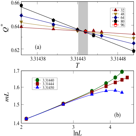
Figure 2: Locating $T_{c}$ for the 4d XY model. (a) The Binder cumulant $Q$ with finite-size corrections being subtracted, namely $Q^{*}(L,T)=Q(L,T)-b({\rm ln}L)^{-\frac{1}{2}}$, with $b\approx 0.1069$ according to a preferred least-squares fit. The shadow marks $T_{c}$ and its error margin. (b) The magnetization density $m$ rescaled by $L^{-1}$ versus ${\rm ln}L$ around $T_{c}=3.314\,44$ in a log-log scale.

By analyzing the finite-size correction $Q(L,T_{c})-Q_{c}$, we find that the leading correction is nearly proportional to $({\rm ln}L)^{-1/2}$, consistent with the prediction of (11) and (12). We let $Q_{c}$ be free in the fits and have $Q_{c}=0.45(1)$, close to the complete-graph result $Q_{c}=0.456\,947$. Besides, we perform simulations for the XY and Heisenberg models on the complete graph and obtain as $Q_{c}\approx 0.635$ and $0.728$, respectively, also close to the fitting results of the 4d $Q$ data. We obtain $T_{c}({\rm XY})=3.314\,437(6)$, and Fig. 2(a) illustrates the location of $T_{c}$ by $Q$.

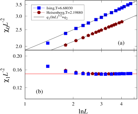
Figure 3: The magnetic fluctuations $\chi_{0}$ (a) and $\chi_{1}$ (b) rescaled by $L^{2}$ versus ${\rm ln}L$ in a log-log scale for the critical Ising and Heisenberg models. The black lines in (a) represent the least-squares fits, and the red one in (b) denotes a constant.

We further examine the estimate of $T_{c}$ by the FSS of other quantities such as the magnetization density $m$. For the XY model, Fig. 2(b) gives a log-log plot of the $mL$ data versus ${\rm ln}L$ for $T=T_{c}$, as well as for $T_{\rm low}=3.314\,40$ and $T_{\rm above}=3.314\,50$. The significant bending-up and -down feature clearly suggests that $T_{\rm low}<T_{c}$ and $T_{\rm above}>T_{c}$, providing confidence for the finally quoted error margin of $T_{c}$.

The final estimates of $T_{c}$ are summarized in Table 1. For $n\!=\!1$, we have $T_{c}=6.680\,300(10)$, which is consonant with and improves over $T_{c}=6.680\,263(23)$ Lundow and Markström (2009) and marginally agrees with $T_{c}=6.679\,63(36)$ Kenna and Lang (1991) and $6.680\,339(14)$ Luijten (1997). For $n\!=\!2$, our determination $T_{c}=3.314\,437(6)$ significantly improves over $T_{c}=3.31$ Jensen et al. (2000a, b) and $3.314$ Nonomura and Tomita (2015). For $n\!=\!3$, our result $T_{c}=2.198\,79(2)$ rules out $T_{c}=2.192(1)$ from a high-temperature expansion McKenzie et al. (1982).

Table 1: Estimates of $T_{c}$ for the 4d O($n$) vector models.

Model	$T_{c}$	Ref.
Ising ($n=1$)	$6.679\,63(36)$	Kenna and Lang (1991)
	$6.680\,339(14)$	Luijten (1997)
	$6.680\,263(23)$	Lundow and Markström (2009)
	$6.680\,300(10)$	this work
XY ($n=2$)	$3.31$,   $3.314$	Jensen et al. (2000a, b); Nonomura and Tomita (2015)
	$3.314\,437(6)$	this work
Heisenberg ($n=3$)	$2.192(1)$	McKenzie et al. (1982)
	$2.198\,79(2)$	this work

III.2 Finite-size scaling of the two-point correlation

We then fit the critical two-point correlation $g(L/2,L)$ to

$$\leavevmode\nobreak\ g(L/2,L)=v_{1}L^{-2}({\rm ln}L)^{\hat{p}}+v_{2}L^{-2},$$ (14)

where the first term comes from the large-distance plateau and the second one is from the $r$-dependent behavior of $g(r,L)$. With $\hat{p}=1/2$ being fixed, the estimate of leading scaling term $L^{-1.98(4)}$ agrees well with the exact $L^{-2}$. With the exponent $-2$ in $L^{-2}$ being fixed, the result $\hat{p}=0.5(1)$ is also well consistent with the prediction $\hat{p}=1/2$. These results are elaborated in the SM.

We remark that FSS analyses for $g(L/2,L)$ have already been performed in Kenna and Berche (2014) with the formula $g(L/2,L)=AL^{-2}[{\rm ln}(L/2+B)]^{1/2}$ ($A$ and $B$ are constants) and in Luijten (1997) with a similar formula. These FSS in literature correspond to the first scaling term in Eq. (14). Hence, formula (14) serves as a forward step for complete FSS by involving the scaling term $v_{2}L^{-2}$, which arises from the Gaussian fixed point.

III.3 Finite-size scaling of the magnetic susceptibility

According to (11) and (12), we fit the critical susceptibility $\chi_{0}$ to

$$\leavevmode\nobreak\ \chi_{0}=q_{1}L^{2}({\rm ln}L)^{\hat{p}}+q_{2}L^{2},$$ (15)

with $q_{1}$ and $q_{2}$ non-universal constants. For $\hat{p}=1/2$ being fixed, we obtain fitting results with $\chi^{2}/{\rm DF}\lesssim 1$ for each of $n\!=\!1,2,3$, and correctly produce the leading scaling form $L^{2}$. The scaled susceptibility $\chi_{0}L^{-2}$ versus ${\rm ln}L$ are demonstrated by Figs. 1(c) (XY) and 3(a) (Ising and Heisenberg).

We note that previous studies based on a FSS without high-order corrections produced estimates of ${\hat{y}}_{h}$ $(=\hat{p}/2)$, considered to be consistent with ${\hat{y}}_{h}=1/4$ Lai and Mon (1990); Kenna and Lang (1991, 1993, 1994). The maximum lattice size therein was $L_{\rm max}=24$, four times smaller than $L_{\rm max}=96$ of the present study. In particular, it was reported Lai and Mon (1990) that $2\hat{y}_{h}=0.45(8)$ and $4\hat{y}_{h}=0.80(25)$. Nevertheless, we find that the fit $\chi_{0}=q_{1}L^{2}({\rm ln}L)^{2\hat{y}_{h}}$ by dropping the correction term $q_{2}L^{2}$ would yield $\hat{y}_{h}=0.21(1)$ (Ising), $0.20(1)$ (XY), and $0.19(1)$ (Heisenberg), which are smaller than and inconsistent with the predicted value $\hat{y}_{h}=1/4$. This suggests the significance of $q_{2}L^{2}$ in the susceptibility $\chi_{0}$, which arises from the $r$-dependence of $g(r,L)$.

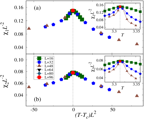
Figure 4: Data collapses for the magnetic fluctuations $\chi_{1}$ (a) and $\chi_{2}$ (b) rescaled by $L^{2y_{h}-d}$ and $L^{y_{t}}$ ($y_{h}=3$, $y_{t}=2$, $d=4$) for the 4d XY model. The insets show the scaled fluctuations versus $T$, and the dashed lines denote $T_{c}$.

III.4 Finite-size scaling of the magnetic fluctuations at non-zero Fourier modes

We consider the magnetic fluctuations $\chi_{1}$ with $|{\bf k}_{1}|=2\pi/L$ and $\chi_{2}$ with $|{\bf k}_{2}|=2\sqrt{2}\pi/L$. We have compared the FSS of $\chi_{0}$, $\chi_{1}$ and $\chi_{2}$ in Figs. 1(c) and (d) for the critical 4d XY model. As $L$ increases, $\chi_{1}L^{-2}$ and $\chi_{2}L^{-2}$ converge rapidly, suggesting the absence of multiplicative logarithmic correction. This is in sharp contrast to the behavior of $\chi_{0}L^{-2}$, which diverges logarithmically. For the Ising and Heisenberg models, the FSS of the fluctuations at non-zero modes is also free of multiplicative logarithmic correction (Fig. 3(b)).

Surprisingly, it is found that the scaled fluctuations $\chi_{1}L^{-2}\approx 0.15$ are equal within error bars for the Ising, XY, and Heisenberg models.

Further, we show in Fig. 4 $\chi_{1}$ and $\chi_{2}$ versus $T$ for the 4d XY model. It is observed that the magnetic fluctuations at non-zero Fourier modes reach maximum at $T_{c}$ and that the $\chi_{1}L^{-2}$ ($\chi_{2}L^{-2}$) data for different $L$s collapse well not only at $T_{c}$ but also for a wide range of $(T-T_{c})L^{y_{t}}$ with $y_{t}=2$.

IV Discussions

We propose formulae (11) and (12) for the FSS of the O($n$) universality class at the upper critical dimensionality, which are tested against extensive MC simulations with $n\!=\!1,2,3$. From the FSS of the magnetic fluctuations at zero and non-zero Fourier modes, the two-point correlation function, and the Binder cumulant, we obtain complementary and solid evidence supporting (11) and (12). As byproducts, the critical temperatures for $n\!=\!1,2,3$ are all located up to an unprecedented precision.

An immediate application of (12) is to the massive amplitude excitation mode (often called the Anderson-Higgs boson) due to the spontaneous breaking of the continuous O($n$) symmetry Pekker and Varma (2015), which is at the frontier of condensed matter research. At the pressure-induced quantum critical point (QCP) in the dimerized quantum antiferromagnet TlCuCl₃, the 3D O(3) amplitude mode was probed by neutron spectroscopy and a rather narrow peak width of about 15% of the excitation energy was revealed, giving no evidence for the logarithmic reduction of the width-mass ratio Merchant et al. (2014). This was later confirmed by quantum MC study of a 3D model Hamiltonian of O(3) symmetry Lohöfer and Wessel (2017); Qin et al. (2017). Indeed, (12) provides an explanation why the logarithmic-correction reduction in the Higgs resonance was not observed at 3D QCP. In numerical studies of the Higgs excitation mode at 3D QCP, the correlation function $g(\tau\!\equiv\!|\tau_{1}\!-\!\tau_{2}|)$ is measured along the imaginary-time axis $\beta$, and numerical analytical continuation is used to deal with the $g(\tau)$ data. In practice, simulations are carried out at very low temperature $\beta\!\rightarrow\!\infty$, and it is expected that $g(\tau)\!\asymp\!\tau^{-2}$ for a significantly wide range of $\tau$. Furthermore, it is the $\tau$-dependent behavior of $g(\tau)$, instead of the $L$-dependence, that plays a decisive role in numerical analytical continuation.

In the thermodynamic limit, the two-point correlation function decays as $g(r)\sim r^{-2}\tilde{g}(r/\xi)$, where the scaling function $\tilde{g}(r/\xi)$ quickly drops to zero as $r/\xi\gg 1$. It can be seen that no multiplicative logarithmic correction exists in the algebraic decaying behavior. On the other hand, as the criticality is approached ($t\!\rightarrow\!0$), the correlation length diverges as $\xi(t)\!\sim\!t^{-1/2}|{\rm ln}t|^{\hat{\nu}}$, and $\hat{\nu}\!=\!\frac{n+2}{2(n+8)}\!>\!0$ implies that $\xi$ diverges faster than $t^{-1/2}$ Kenna (2004, 2012). Since the susceptibility can be calculated by summing up the correlation as $\chi_{0}\sim\int_{0}^{\xi}g(r)r^{d-1}dr\sim\xi^{2}$, one has $\chi_{0}(t)\sim t^{-1}|\ln t|^{\hat{\gamma}}$ with $\hat{\gamma}=2\hat{\nu}$. The thermodynamic scaling of $\chi_{0}(t)$ can also be obtained from the FSS formula (10) or (11), which gives $\chi_{0}(t,L)\sim L^{2y_{h}-4}(\ln L)^{2\hat{y}_{h}}\tilde{\chi_{0}}(tL^{y_{t}}(\ln L)^{\hat{y}_{t}})$. By fixing $tL^{y_{t}}(\ln L)^{\hat{y}_{t}}$ at some constant, one obtains the relation $L\sim t^{-1/y_{t}}|\ln t|^{-\hat{y}_{t}/y_{t}}$. Substituting it into the FSS of $\chi_{0}(t,L)$ yields $\chi_{0}(t)\sim t^{\gamma}|\ln t|^{\hat{\gamma}}$ with $\gamma\!=\!(2y_{h}-4)/y_{t}$ and $\hat{\gamma}\!=\!-\gamma\hat{y}_{t}+2\hat{y}_{h}$. With $(y_{t},y_{h},\hat{y}_{t},\hat{y}_{h})=(2,3,\frac{4-n}{2n+16},\frac{1}{4})$, one has $\gamma=1$ and $\hat{\gamma}=\frac{n+2}{n+8}$. The thermodynamic scaling with logarithmic corrections has been demonstrated in Ref. Qin et al. (2015) in terms of the magnetization $m$ of an O(3) Hamiltonian.

For the critical Ising model in five dimensions, an unwrapped distance $r_{\rm u}$ was introduced to account for the winding numbers across a finite torus Grimm et al. (2017). The unwrapped correlation was shown to behave as $g(r_{\rm u})\sim r_{\rm u}^{2-d}\tilde{g}(r_{\rm u}/\xi_{\rm u})$, where the unwrapped correlation length diverges as $\xi_{\rm u}\sim L^{d/4}$. This differs from typical correlation functions that are cut off by the linear system size $\sim L$. We expect that at $d_{c}=4$, the unwrapped correlation length diverges as $\xi_{\rm u}\sim L(\ln L)^{\hat{y}_{h}}$, which gives the critical susceptibility as $\chi_{0}(L)\sim L^{2}(\ln L)^{2\hat{y}_{h}}$.

Besides, formula (12) is useful for predicting various critical behaviors. As an instance, it was observed that an impurity immersed in a 2D O(2) quantum critical environment can evolve into a quasiparticle of fractionalized charge, as the impurity-environment interaction is tuned to a boundary critical point Huang et al. (2016); Whitsitt and Sachdev (2017); Chen et al. (2018). Formula (12) precludes the emergence of such a quantum-fluctuation-induced quasiparticle at 3D O(2) QCP.

We mention an open question about the specific heat of the 4d Ising model. FSS formula (10) predicts that the critical specific heat diverges as $C\!\asymp\!(\ln L)^{1/3}$. By contrast, a MC study demonstrated that the critical specific heat is bounded Lundow and Markström (2009). The complete scaling form (11) is potentially useful for reconciling the inconsistence.

Finally, it would be possible to extend the present scheme to other systems of critical phenomena, as the existence of upper critical dimensionality is a common feature therein. These systems include the percolation and spin-glass models at their upper critical dimensionality $d_{c}=6$. We leave this for a future study.

V Method

Throughout the paper, the raw data for any temperature $T$ and linear size $L$ are obtained by means of MC simulations, for which the Wolff cluster algorithm Wolff (1989) and the Prokof’ev-Svistunov worm algorithm Prokof’ev and Svistunov (2001) are employed complementarily. Both algorithms are state-of-the-art tools in their own territories.

The O($n$) vector model (1) in its original spin representation is efficiently sampled by the Wolff cluster algorithm, which is the single-cluster version of the widely utilized non-local cluster algorithms. The present study uses the standard procedure of the algorithm, as in the original paper Wolff (1989) where the algorithm was invented. In some situations, we also use the conventional Metropolis algorithm Metropolis et al. (1953) for benchmarks. The macroscopic physical quantities of interest have been introduced in aforementioned sections for the spin representation.

The two-point correlation function for the XY model ($n=2$) is sampled by means of the Prokof’ev-Svistunov worm algorithm, which was invented for a variety of classical statistical models Prokof’ev and Svistunov (2001). By means of a high-temperature expansion, we perform an exact transformation for the original XY spin model to a graphic model in directed-flow representation. We then introduce two defects for enlarging the state space of directed flows. The Markov chain process of evolution is built upon biased random walks of defects, which satisfy the detailed balance condition. It is defined that the evolution hits the original directed-flow state space when the two defects meet at a site. The details for the exact transformation and a step-by-step procedure for the algorithm have been presented in a recent reference Xu et al. (2019).

VI Conflict of interest statement

None declared.

References

- Fernández et al. (2013) R. Fernández, J. Fröhlich, and A. D. Sokal, Random walks, critical phenomena, and triviality in quantum field theory (Springer, Berlin, 2013).
- Svistunov et al. (2015) B. V. Svistunov, E. S. Babaev, and N. V. Prokof’ev, Superfluid states of matter (CRC Press, London, 2015).
- Merchant et al. (2014) P. Merchant, B. Normand, K. W. Krämer, M. Boehm, D. F. McMorrow, and Ch. Rüegg, “Quantum and classical criticality in a dimerized quantum antiferromagnet,” Nat. Phys. 10, 373–379 (2014).
- Qin et al. (2015) Y. Q. Qin, B. Normand, A. W. Sandvik, and Z. Y. Meng, “Multiplicative logarithmic corrections to quantum criticality in three-dimensional dimerized antiferromagnets,” Phys. Rev. B 92, 214401 (2015).
- Lohöfer and Wessel (2017) M. Lohöfer and S. Wessel, “Excitation-gap scaling near quantum critical three-dimensional antiferromagnets,” Phys. Rev. Lett. 118, 147206 (2017).
- Qin et al. (2017) Y. Q. Qin, B. Normand, A. W. Sandvik, and Z. Y. Meng, “Amplitude mode in three-dimensional dimerized antiferromagnets,” Phys. Rev. Lett. 118, 147207 (2017).
- Cui et al. (2019) Y. Cui, H. Zou, N. Xi, Z. He, Y. X. Yang, L. Shu, G. H. Zhang, Z. Hu, T. Chen, R. Yu, J. Wu, and W. Yu, “Quantum criticality of the ising-like screw chain antiferromagnet in a transverse magnetic field,” Phys. Rev. Lett. 123, 067203 (2019).
- Resnick et al. (1981) D. J. Resnick, J. C. Garland, J. T. Boyd, S. Shoemaker, and R. S. Newrock, “Kosterlitz-thouless transition in proximity-coupled superconducting arrays,” Phys. Rev. Lett. 47, 1542–1545 (1981).
- Goldman (2013) A. Goldman, Percolation, localization, and superconductivity, Vol. 109 (Springer, Boston, 2013).
- Greiner et al. (2002) M. Greiner, O. Mandel, T. Esslinger, T. W. Hänsch, and I. Bloch, “Quantum phase transition from a superfluid to a mott insulator in a gas of ultracold atoms,” Nature 415, 39–44 (2002).
- Capogrosso-Sansone et al. (2007) B. Capogrosso-Sansone, N. V. Prokof’ev, and B. V. Svistunov, “Phase diagram and thermodynamics of the three-dimensional bose-hubbard model,” Phys. Rev. B 75, 134302 (2007).
- Cardy (2012) J. Cardy, Finite-size scaling, Vol. 2 (Elsevier, Amsterdam, 2012).
- Luijten (1997) E. Luijten, Interaction range, universality and the upper critical dimension (Delft University Press, Delft, 1997).
- Luijten et al. (1999) E. Luijten, K. Binder, and H. W. J. Blöte, “Finite-size scaling above the upper critical dimension revisited: the case of the five-dimensional ising model,” Euro. Phys.J. B 9, 289–297 (1999).
- Wittmann and Young (2014) M. Wittmann and A. P. Young, “Finite-size scaling above the upper critical dimension,” Phys. Rev. E 90, 062137 (2014).
- Kenna and Berche (2014) R. Kenna and B. Berche, “Fisher’s scaling relation above the upper critical dimension,” EPL (Europhysics Letters) 105, 26005 (2014).
- Flores-Sola et al. (2016) E. Flores-Sola, B. Berche, R. Kenna, and M. Weigel, “Role of fourier modes in finite-size scaling above the upper critical dimension,” Phys. Rev. Lett. 116, 115701 (2016).
- Grimm et al. (2017) J. Grimm, E. M. Elçi, Z. Zhou, T. M. Garoni, and Y. Deng, “Geometric explanation of anomalous finite-size scaling in high dimensions,” Phys. Rev. Lett. 118, 115701 (2017).
- Papathanakos (2006) V. Papathanakos, Finite-size effects in high-dimensional statistical mechanical systems: The Ising model with periodic boundary conditions (Ph.D. thesis, Princeton University, Princeton, New Jersey, 2006).
- Zhou et al. (2018) Z. Zhou, J. Grimm, S. Fang, Y. Deng, and T. M. Garoni, “Random-length random walks and finite-size scaling in high dimensions,” Phys. Rev. Lett. 121, 185701 (2018).
- Fang et al. (2019) S. Fang, J. Grimm, Z. Zhou, and Y. Deng, “Anomalous finite-size scaling in the fortuin-kasteleyn clusters of the five-dimensional ising model with periodic boundary conditions,” arXiv:1909.04328 (2019).
- Fisher (1971) M. E. Fisher, Critical Phenomena, Proceedings of the 51st Enrico Fermi Summer School, Varenna, Italy, edited by M. S. Green (Academic, New York, 1971).
- Binder et al. (1985) K. Binder, M. Nauenberg, V. Privman, and A. P. Young, “Finite-size tests of hyperscaling,” Phys. Rev. B 31, 1498 (1985).
- Berche et al. (2012) B. Berche, R. Kenna, and J.-C. Walter, “Hyperscaling above the upper critical dimension,” Nucl. Phys. B 865, 115–132 (2012).
- Kenna and Berche (2013) R. Kenna and B. Berche, “A new critical exponent koppa and its logarithmic counterpart koppa-hat,” Cond. Matt. Phys. 16, 23601 (2013).
- Aizenman (1982) M. Aizenman, “Geometric analysis of 4 fields and ising models. parts i and ii,” Commun. Math. Phys. 86, 1–48 (1982).
- Aizenman (1985) M. Aizenman, Rigorous studies of critical behavior II, Statistical Physics and Dynamical Systems: Rigorous Results, edited by J. Fritz, A. Jaffe, D. Szasz. (Birkhauser, Boston, 1985).
- Aizenman (1986) M. Aizenman, “Rigorous studies of critical behavior,” Physica A 140, 225–231 (1986).
- Huang et al. (2018) W. Huang, P. Hou, J. Wang, R. M. Ziff, and Y. Deng, “Critical percolation clusters in seven dimensions and on a complete graph,” Phys. Rev. E 97, 022107 (2018).
- Kenna (2004) R. Kenna, “Finite size scaling for o(n) -theory at the upper critical dimension,” Nucl. Phys. B 691, 292–304 (2004).
- Aktekin (2001) N. Aktekin, “The finite-size scaling functions of the four-dimensional ising model,” J. Stat. Phys. 104, 1397–1406 (2001).
- Wegner and Riedel (1973) F. J. Wegner and E. K. Riedel, “Logarithmic corrections to the molecular-field behavior of critical and tricritical systems,” Phys. Rev. B 7, 248 (1973).
- Kenna (2012) R. Kenna, Universal scaling relations for logarithmic-correction exponents, Order, Disorder and Criticality, Advanced Problems of Phase Transition Theory, edited by Y. Holovatch (World Scientific, New York, 2012).
- Slade and Tomberg (2016) G. Slade and A. Tomberg, “Critical correlation functions for the 4-dimensional weakly self-avoiding walk and n-component model,” Commun. Math. Phys 342, 675–737 (2016).
- Wolff (1989) U. Wolff, “Collective monte carlo updating for spin systems,” Phys. Rev. Lett. 62, 361 (1989).
- Prokof’ev and Svistunov (2001) N. V. Prokof’ev and B. V. Svistunov, “Worm algorithms for classical statistical models,” Phys. Rev. Lett. 87, 160601 (2001).