Entanglement-Assisted Capacity of Quantum Channels with Side Information

Abstract

Entanglement-assisted communication over a random-parameter quantum channel with either causal or non-causal channel side information (CSI) at the encoder is considered. This describes a scenario where the quantum channel depends on the quantum state of the input environment. While Bob, the decoder, has no access to this state, Alice, the transmitter, performs a sequence of projective measurements on her environment to encode her message. Dupuis [25, 26] established the entanglement-assisted capacity with non-causal CSI. Here, we establish characterization in the causal setting, and also give an alternative proof technique and further observations for the non-causal setting.

I Introduction

A fundamental task in classical information theory is to determine the ultimate transmission rate of communication. Shannon’s channel coding theorem [58] states that for a given noisy channel, with a transition probability function $p_{Y|X}$, a vanishing probability of error is achievable as long as the transmission rate is lower than the channel capacity, given by $C(p_{Y|X})=\max_{p_{X}}I(X;Y)$, where $I(X;Y)$ is the mutual information between the channel input $X$ and output $Y$. For rates above the channel capacity, reliable communication cannot be accomplished.

Various classical settings of practical significance can be described by a channel $p_{Y|X,S}$ that depends on a random parameter $S$ when there is causal or non-causal channel side information (CSI) available at the encoder (see e.g. [39, 41, 15] and references therein). For example, a cognitive radio in a wireless system may be aware of the channel state and network configuration [29, 32, 64], memory storage where the writer knows the fault locations [33, 48], and digital watermarking where the host data is treated as side information (see e.g. [12, 65, 52]). The capacity with causal CSI is given by [59]

$$C_{E,\text{caus}}(p_{Y|X,S})=\max_{p_{T}}I(T;Y)$$ (1)

with $X=T(S)$, where $T:\mathcal{S}\rightarrow\mathcal{X}$ is called a Shannon strategy (see also [41, 15]). A channel with non-causal CSI is often referred to as the Gel’fand-Pinsker model [28]. The capacity of this channel is given by

$$C_{E,\text{n-c}}(p_{Y|X,S})=\max_{p_{U,X|S}}[I(U;Y)-I(U;S)]$$ (2)

where $U$ is an auxiliary random variable.

The field of quantum information is rapidly evolving in both practice and theory [24, 40, 6, 46, 5, 72, 49, 73]. As technology approaches the atomic scale, we seem to be on the verge of the “Quantum Age” [10, 38]. Dynamics can sometimes be modeled by a noisy quantum channel, describing physical evolutions, density transformation, discarding of sub-systems, quantum measurements, etc [47] [67, Section 4.6]. Quantum information theory is the natural extension of classical information theory. Nevertheless, this generalization reveals astonishing phenomena with no parallel in classical communication [30]. For example, two quantum channels, each with zero quantum capacity, can have a nonzero quantum capacity when used together [63]. This property is known as super-activation.

Communication through quantum channels can be separated into different categories. In particular, one may consider a setting where Alice and Bob are provided with entanglement resources [53]. The entanglement-assisted capacity for transmission of classical information over a quantum channel was fully characterized by Bennet et al. [7, 8]. Further work on entanglement-assisted communication can be found e.g. in [35, 37, 23, 60, 17, 68, 54, 2, 11, 3]. As for classical communication without entanglement between the encoder and the decoder, the Holevo-Schumacher-Westmoreland (HSW) Theorem provides an asymptotic (“multi-letter”) formula for the capacity [34, 57], though calculation of such a formula is intractable in general. This is because the Holevo information is not necessarily additive [31]. Shor has shown that the Holevo information is additive for the class of entanglement-breaking channels [62], in which case the HSW theorem provides a single-letter computable formula for the classical capacity. This class includes both classical-quantum channels and quantum-classical channels [67, Section 4.6.7]. A similar difficulty occurs with transmission of quantum information over a quantum channel. A multi-letter formula for the quantum capacity is given in [4, 50, 61, 20], in terms of the coherent information. A computable formula is obtained in the special case where the channel is degradable [21].

The entanglement-assisted capacity of a quantum channel with non-causal CSI was determined by Dupuis [25, 26]. Furthermore, Boche, Cai, and Nötzel [9] addressed the classical-quantum channel with CSI at the encoder without entanglement. The classical capacity was determined given causal CSI, and a multi-letter formula was provided given non-causal CSI. Warsi and Coon [66] used an information-spectrum approach to derive multi-letter bounds for a similar setting, where the side information has a limited rate. Luo and Devetak [51] considered channel simulation with source side information (SSI) at the decoder, and also solved the quantum generalization of the Wyner-Ziv problem [70]. Quantum data compression with SSI is also studied in [22, 71, 36, 19, 18, 14, 13] without entanglement-assitance. Compression with SSI given entanglement assistance was recently considered by Khanian and Winter [45, 42, 44, 43].

In this paper, we consider a quantum channel with either causal or non-causal CSI. The motivation is as follows. Suppose that Alice wishes to send classical information to Bob through a (fully) quantum channel $\mathcal{N}_{SA\rightarrow B}$, where $A$ is the transmitter system, $B$ is the receiver system, and $S$ is the transmitter’s environment, which affects the channel as well. Furthermore, suppose that Alice performs a sequence of projective measurements of the environment system $S$, hence the system is projected onto a particular vector $|s\rangle$ with probability $q(s)$. Using the measurement results, Alice encodes her message and sends her transmission through the channel. Whereas, Bob, who does not have access to the measurement results, “sees” the average channel $\sum_{s}q(s)\mathcal{N}^{(s)}_{A\rightarrow B}$, where $\mathcal{N}^{(s)}_{A\rightarrow B}$ is the projection of the channel onto $|s\rangle$. Assuming Alice’s measurement projects onto orthogonal vectors, the environment system can be thought of as a classical random parameter $S\sim q(s)$. Therefore, we treat the quantum counterpart of the models in [59] and [28], i.e. a random-parameter quantum channel $\mathcal{N}_{SA\rightarrow B}$ with CSI at the encoder.

We give a full characterization of the entanglement-assisted classical capacity and quantum capacity with causal CSI, and also give an alternative proof technique and further observations for the non-causal setting. While Dupuis’ analysis with non-causal CSI in [25, 26] is based on the decoupling approach for the transmission of quantum information (qubits), we take a more direct approach. In our analysis, we incorporate the classical binning technique [33] into the quantum packing lemma [37]. Essentially, in the achievability proof, Alice performs classical compression of the parameter sequence, and then transmits both the classical message and the compressed representation using a random phase variation of the superdense coding protocol (see e.g. [37, 67]). The results are analogous to those in the classical case, although, as usual, the quantum analysis is more involved. As observed in [28, 33], the classical optimization (2) can be restricted to mappings from $(U,S)$ to $X$ that are deterministic. In analogy, we observe that optimization over isometric maps suffices for our problem. With causal CSI, quantum operations are applied in a reversed order, and the Shannon strategy in (1) is replaced with a quantum channel.

II Definitions and Related Work

We begin with basic definitions.

II-A Notation, States, and Information Measures

We use the following notation conventions. Calligraphic letters $\mathcal{X},\mathcal{Y},\mathcal{Z},...$ are used for finite sets. Lowercase letters $x,y,z,\ldots$ represent constants and values of classical random variables, and uppercase letters $X,Y,Z,\ldots$ represent classical random variables. The distribution of a random variable $X$ is specified by a probability mass function (pmf) $p_{X}(x)$ over a finite set $\mathcal{X}$. We use $x^{j}=(x_{1},x_{2},\ldots,x_{j})$ to denote a sequence of letters from $\mathcal{X}$. A random sequence $X^{n}$ and its distribution $p_{X^{n}}(x^{n})$ are defined accordingly. For a pair of integers $i$ and $j$, $1\leq i\leq j$, we write a discrete interval as $[i:j]=\{i,i+1,\ldots,j\}$.

The state of a quantum system $A$ is given by a density operator $\rho$ on the Hilbert space $\mathcal{H}_{A}$. A density operator is an Hermitian, positive semidefinite operator, with unit trace, i.e. $\rho^{\dagger}=\rho$, $\rho\succeq 0$, and $\mathrm{Tr}(\rho)=1$. The state is said to be pure if $\rho=|\psi\rangle\langle\psi|$, for some vector $|\psi\rangle\in\mathcal{H}_{A}$, where $\langle\psi|$ is the Hermitian conjugate of $|\psi\rangle$. In general, a density operator has a spectral decomposition of the following form,

$$\rho=\sum_{z\in\mathcal{Z}}p_{Z}(z)|\psi_{z}\rangle\langle\psi_{z}|$$ (3)

where $\mathcal{Z}=\{1,2,\ldots,|\mathcal{H}_{A}|\}$, $p_{Z}(z)$ is a probability distribution over $\mathcal{Z}$, and $\{|\psi_{z}\rangle\}_{z\in\mathcal{Z}}$ forms an orthonormal basis of the Hilbert space $\mathcal{H}_{A}$. The density operator can thus be thought of as an average of pure states. A measurement of a quantum system is any set of operators $\{\Lambda_{j}\}$ that forms a positive operator-valued measure (POVM), i.e. the operators are positive semi-definite and $\sum_{j}\Lambda_{j}=\text{1}$, where 1 is the identity operator (see [67, Definition 4.2.1]). According to the Born rule, if the system is in state $\rho$, then the probability of the measurement outcome $j$ is given by $p_{A}(j)=\mathrm{Tr}(\Lambda_{j}\rho)$.

Define the quantum entropy of the density operator $\rho$ as

$$H(\rho)\triangleq -\mathrm{Tr}[\rho\log(\rho)]$$ (4)

which is the same as the Shannon entropy associated with the eigenvalues of $\rho$. We may also consider the state of a pair of systems $A$ and $B$ on the tensor product $\mathcal{H}_{A}\otimes\mathcal{H}_{B}$ of the corresponding Hilbert spaces. Given a bipartite state $\sigma_{AB}$, define the quantum mutual information by

$$I(A;B)_{\sigma}=H(\sigma_{A})+H(\sigma_{B})-H(\sigma_{AB})\,.$$ (5)

Furthermore, conditional quantum entropy and mutual information are defined by $H(A|B)_{\sigma}=H(\sigma_{AB})-H(\sigma_{B})$ and $I(A;B|C)_{\sigma}=H(A|C)_{\sigma}+H(B|C)_{\sigma}-H(A,B|C)_{\sigma}$, respectively.

A pure bipartite state is called entangled if it cannot be expressed as the tensor product of two states in $\mathcal{H}_{A}$ and $\mathcal{H}_{B}$. The maximally entangled state between two systems of dimension $D$ is defined by $|\Phi_{AB}\rangle=\frac{1}{\sqrt{D}}\sum_{j=0}^{D-1}|j\rangle_{A}\otimes|j\rangle_{B}$, where $\{|j\rangle_{A}\}_{j=0}^{D-1}$ and $\{|j\rangle_{B}\}_{j=0}^{D-1}$ are respective orthonormal bases. Note that $I(A;B)_{|\Phi\rangle\langle\Phi|}=2\cdot\log(D)$.

II-B Quantum Channel

A quantum channel maps a quantum state at the sender system to a quantum state at the receiver system. Here, we consider a channel that is governed by a random parameter with a particular distribution. Formally, a random-parameter quantum channel is defined as a linear, completely positive, trace preserving map $\mathcal{N}_{SA\rightarrow B}$, corresponding to a quantum physical evolution. The channel parameter $S$ can also be thought of as a classical system at state

$$\rho_{S}=\sum_{s\in\mathcal{S}}q(s)|s\rangle\langle s|$$ (6)

where $\{|s\rangle\}_{s\in\mathcal{S}}$ is an orthonormal basis of the Hilbert space $\mathcal{H}_{S}$. A quantum channel has a Kraus representation

$$\mathcal{N}_{SA\rightarrow B}(\rho)=\sum_{j}N_{j}\rho_{SA}N_{j}^{\dagger}$$ (7)

for all $\rho_{SA}$, where the operators $N_{j}$ satisfy $\sum_{j}N_{j}^{\dagger}N_{j}=\text{1}$ [67, Section 4.4.1]. The projection on $|s\rangle$ is then given by

$$\mathcal{N}^{(s)}_{A\rightarrow B}(\rho)=\sum_{j}N_{j}^{(s)}\rho N_{j}^{(s)\,\dagger}$$ (8)

where $N_{j}^{(s)}\equiv\langle s|N_{j}|s\rangle$. A quantum channel is called isometric if it can be expressed as $\mathcal{N}_{SA\rightarrow B}(\rho)=N\rho_{SA}N^{\dagger}$ where the operator $N$ is an isometry, i.e. $N^{\dagger}N=\text{1}$ [67, Section 4.6.3].

We assume that both the random parameter state and the quantum channel have a product form. That is, the state of the joint system $S^{n}=(S_{1},\ldots,S_{n})$ is $\rho_{S^{n}}=\rho_{S}^{\otimes n}$, and if the systems $A^{n}=(A_{1},\ldots,A_{n})$ are sent through $n$ channel uses, then the parameter-input state $\rho_{S^{n}}\otimes\rho_{A^{n}}$ undergoes the tensor product mapping $\mathcal{N}_{S^{n}A^{n}\rightarrow B^{n}}\equiv\mathcal{N}_{SA\rightarrow B}^{\otimes n}$. Therefore, without CSI, the input-output relation is

$$\rho_{B^{n}}=\sum_{s^{n}\in\mathcal{S}^{n}}q^{n}(s^{n})\mathcal{N}^{(s^{n})}_{A^{n}\rightarrow B^{n}}(\rho_{A^{n}})=\left(\sum_{s\in\mathcal{S}}q(s)\mathcal{N}^{(s)}_{A\rightarrow B}\right)^{\otimes n}(\rho_{A^{n}})$$ (9)

where $q^{n}(s^{n})=\prod_{i=1}^{n}q(s_{i})$ is the joint distribution of the parameter sequence and $\mathcal{N}^{(s^{n})}_{A^{n}\rightarrow B^{n}}=\mathcal{N}^{(s_{1})}_{A\rightarrow B}\otimes\cdots\otimes\mathcal{N}^{(s_{n})}_{A\rightarrow B}$. The sender and the receiver are often referred to as Alice and Bob.

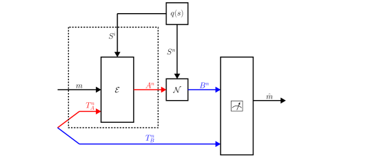
Figure 1: Coding for a quantum channel $\mathcal{N}_{SA\rightarrow B}$ that depends on a random parameter $S\sim q(s)$, with causal side information at the encoder. The quantum systems of Alice and Bob are marked in red and blue, respectively. In particular, the systems inside the dashed-line rectangle are only available at the encoder. Alice chooses a classical message $m$. At time $i$, given the parameter sequence $s^{i}$, she applies the encoding channel $\mathcal{E}^{m,s^{i}}_{T_{A,i}\rightarrow A_{i}}$ to her share of the entangled state $\Psi_{T_{A,i},T_{B,i}}$, and then transmits the system $A_{i}$ over the quantum channel $\mathcal{N}_{SA\rightarrow B}$. Bob receives the channel output systems $B^{n}$, combines them with the entangled system $T_{B}^{n}$, and performs a measurement. The outcome is the estimated message $\hat{m}$.

II-C Coding

We define a code to transmit classical information provided that the encoder and the decoder share unlimited entanglement. The entangled system pairs are denoted by $(T_{A}^{n},T_{B}^{n})=(T_{A,i},T_{B,i})_{i=1}^{n}$. With causal CSI, Alice knows the sequence of past and present random parameters, $S_{1},\ldots,S_{i}$, at $i\in[1:n]$.

Definition 1.

A $(2^{nR},n)$ entanglement-assisted classical code with causal CSI at the encoder consists of the following: a message set $[1:2^{nR}]$, where $2^{nR}$ is assumed to be an integer, a pure entangled state $\Psi_{T_{A}^{n},T_{B}^{n}}$, a sequence of $n$ encoding maps (channels) $\mathcal{E}^{m,s^{i}}_{T_{A,i}\rightarrow A_{i}}$, $m\in[1:2^{nR}]$, $s^{i}\in\mathcal{S}^{i}$, for $i\in[1:n]$, and a decoding POVM $\{\Lambda^{m}_{B^{n}T_{B}^{n}}\}_{m\in[1:2^{nR}]}$. We denote the code by $(\mathcal{E},\Psi,\Lambda)$.

The communication scheme is depicted in Figure 1. The sender Alice has the systems $T_{A}^{n},A^{n}$ and the receiver Bob has the systems $T_{B}^{n},B^{n}$, where $T_{A}^{n}$ and $T_{B}^{n}$ are entangled. Alice chooses a classical message $m\in[1:2^{nR}]$. At time $i\in[1:n]$, given the sequence of past and present parameters $s^{i}\in\mathcal{S}^{i}$, she applies the encoding channel $\mathcal{E}^{m,s^{i}}_{T_{A,i}\rightarrow A_{i}}$ to her share of the entangled state $\Psi_{T_{A,i},T_{B,i}}$, and then transmits the system $A_{i}$ over the channel. In other words, Alice uses an encoding channel $\overline{\mathcal{E}}^{m,s^{n}}_{T_{A}^{n}\rightarrow A^{n}}$ of the following form,

$$\overline{\mathcal{E}}^{m,s^{n}}\triangleq\mathcal{E}^{m,s_{1}}\otimes\mathcal{E}^{m,s_{1},s_{2}}\otimes\cdots\otimes\mathcal{E}^{m,s^{n}}\,,$$ (10)

and transmits the systems $A^{n}$ over $n$ channel uses of $\mathcal{N}_{SA\rightarrow B}$.

Bob receives the channel output systems $B^{n}$, combines them with the entangled system $T_{B}^{n}$, and performs the POVM $\{\Lambda^{m}_{B^{n}T_{B}^{n}}\}_{m\in[1:2^{nR}]}$. The conditional probability of error, given that the message $m$ was sent, is given by

$$P_{e|m}^{(n)}(\mathcal{E},\Psi,\Lambda)=\sum_{s^{n}\in\mathcal{S}^{n}}q^{n}(s^{n})\mathrm{Tr}\Big{[}(\text{1}-\Lambda^{m}_{B^{n}T_{B}})(\mathcal{N}^{(s^{n})}_{A^{n}\rightarrow B^{n}}\otimes\text{1})(\overline{\mathcal{E}}^{m,s^{n}}\otimes\text{1})(\Psi_{T_{A}^{n},T_{B}^{n}})\Big{]}\,.$$ (11)

A $(2^{nR},n,\varepsilon)$ entanglement-assisted classical code satisfies $P_{e|m}^{(n)}(\mathcal{E},\Psi,\Lambda)\leq\varepsilon$ for all $m\in[1:2^{nR}]$. A rate $R>0$ is called achievable if for every $\varepsilon>0$ and sufficiently large $n$, there exists a $(2^{nR},n,\varepsilon)$ code. The entanglement-assisted classical capacity $\mathbb{C}_{E,\text{caus}}(\mathcal{N})$ is defined as the supremum of achievable rates.

Next, we give a definition of an entanglement-assisted quantum code. A more general definition can be found in [67].

Definition 2.

A $(2^{nQ},n)$ entanglement-assisted quantum code with causal CSI consists of the following; A quantum state $\rho_{M}^{\otimes n}$, where $M$ is a system of dimension $2^{nQ}$; a pure entangled state $\Psi_{T_{A},T_{B}}$, a sequence of $n$ encoding channels $\mathcal{E}^{s^{i}}_{T_{A,i}M\rightarrow A_{i}}$, and a decoding channel $\mathcal{D}_{B^{n}T_{B}^{n}\rightarrow\hat{M}}$.

The sender Alice has the systems $T_{A}^{n},M,A^{n}$ and the receiver Bob has the systems $T_{B}^{n},B^{n},\hat{M}$, where $T_{A}^{n}$ and $T_{B}^{n}$ are entangled. Alice encodes the state $\rho_{M}$ by applying the encoding channel $\overline{\mathcal{E}}_{M,S^{n},T_{A}^{n}\rightarrow A^{n}}$ to $\rho_{M}^{\otimes n}$ and to her share of the entangled state $\Psi_{T_{A}^{n},T_{B}^{n}}$, where $\overline{\mathcal{E}}_{M,S^{n},T_{A}^{n}\rightarrow A^{n}}=\bigotimes_{i=1}^{n}\mathcal{E}_{M,S^{i},T_{A,i}\rightarrow A_{i}}$, and transmits the system $A^{n}$ over $n$ channel uses of $\mathcal{N}_{SA\rightarrow B}$. Bob receives the channel output systems $B^{n}$, combines them with the entangled system $T_{B}$, and applies the decoding channel $\mathcal{D}_{B^{n}T_{B}^{n}\rightarrow\hat{M}}$. The code is said to be a $(2^{nQ},n,\varepsilon)$ entanglement-assisted quantum code if the trace distance between the original state and the resulting state at the receiver is bounded by

$$\frac{1}{2}\left\lVert\rho_{M}-\mathcal{D}\left(\sum_{s^{n}\in\mathcal{S}^{n}}q^{n}(s^{n})(\mathcal{N}^{(s^{n})}_{A^{n}\rightarrow B^{n}}\otimes\text{1})(\overline{\mathcal{E}}^{s^{n}}\otimes\text{1})\left(\rho_{M}^{\otimes n}\otimes\Psi_{T_{A}^{n},T_{B}^{n}}\right)\right)\right\rVert_{1}\leq\varepsilon\,,$$ (12)

where $\left\lVert\cdot\right\rVert_{1}$ denotes the trace norm. A positive number $Q>0$ is said to be an achievable rate if for every $\varepsilon>0$ and sufficiently large $n$, there exists a $(2^{nQ},n,\varepsilon)$ code. The entanglement-assisted quantum capacity $\mathbb{Q}_{E,\text{caus}}$ is defined as the supremum of achievable rates.

We also discuss the non-causal setting, where Alice has the parameter sequence $S^{n}$ a priori, and can thus applies any encoding channel $\overline{\mathcal{E}}_{M,S^{n},T_{A}^{n}\rightarrow A^{n}}$. In addition, we consider the case where there is CSI at the decoder, i.e. when Bob receives both $B^{n}$ and $S^{n}$, and performs a POVM $\{\Lambda^{m}_{B^{n}S^{n}T_{B}}\}_{m\in[1:2^{nR}]}$. We note that for the decoder, causality is insignificant. We use the respective subscripts ‘$E$’, ‘$D$’ or ‘$ED$’ to indicate that CSI is available at either the encoder, the decoder, or both, and the subscripts ‘caus’ or ‘n-c’ to indicate whether CSI is available at the encoder in a causal or non-causal manner, respectively. The notation is summarized in the table in Figure 2.

	none	encoder	decoder	encoder$+$decoder	encoder (causal)
Classical	$\mathbb{C}(\mathcal{N})$	$\mathbb{C}_{E,\text{n-c}}(\mathcal{N})$	$\mathbb{C}_{D}(\mathcal{N})$	$\mathbb{C}_{ED,\text{n-c}}(\mathcal{N})$	$\mathbb{C}_{E,\text{caus}}(\mathcal{N})$
Quantum	$\mathbb{Q}(\mathcal{N})$	$\mathbb{Q}_{E,\text{n-c}}(\mathcal{N})$	$\mathbb{Q}_{D}(\mathcal{N})$	$\mathbb{Q}_{ED,\text{n-c}}(\mathcal{N})$	$\mathbb{Q}_{E,\text{caus}}(\mathcal{N})$

Figure 2: Notation of channel capacities with and without CSI. The columns correspond to the location where CSI is available, and the rows indicate the type of information capacity – classical or quantum.

II-D Related Work

We briefly review known results for a quantum channel that does not depend on a random parameter, i.e. $\mathcal{N}^{(s)}_{A\rightarrow B}=\mathcal{N}^{(0)}_{A\rightarrow B}$ for $s\in\mathcal{S}$. Define

$$\mathsf{C}(\mathcal{N}^{(0)})\triangleq\max_{|\phi\rangle_{AA^{\prime}}}I(A;B)_{\rho}$$ (13)

with $\rho_{AB}\equiv(\text{1}\otimes\mathcal{N}^{(0)})(|\phi\rangle\langle\phi|_{AA^{\prime}})$. Next, we give the respective capacity theorems for the entanglement-assisted classical capacity and the entanglement-assisted quantum capacity.

Theorem 1 (see [7, 8]).

The entanglement-assisted classical capacity of a quantum channel $\mathcal{N}_{A\rightarrow B}^{(0)}$ is given by

$$\mathbb{C}(\mathcal{N}^{(0)})=\mathsf{C}(\mathcal{N}^{(0)})\,.$$ (14)

Given an unlimited supply of entanglement, the teleportation protocol can send a qubit using two classical bits, while the super-dense coding protocol can send two classical bits using one qubit [53]. This implies the following.

Corollary 2 (see [7, 8]).

The entanglement-assisted quantum capacity of a quantum channel $\mathcal{N}_{A\rightarrow B}^{(0)}$ is given by

$$\mathbb{Q}(\mathcal{N}^{(0)})=\frac{1}{2}\mathsf{C}(\mathcal{N}^{(0)})\,.$$ (15)

Remark 1.

We note that the setting of a random-parameter quantum channel $\mathcal{N}_{SA\rightarrow B}$ without side information is equivalent to that of a channel that does not depend on a state, with $\mathcal{N}_{A\rightarrow B}^{(0)}=\sum_{s\in\mathcal{S}}q(s)\mathcal{N}_{A\rightarrow B}^{(s)}$ (see (9)). On the other hand, with side information at the encoder, this equivalence does not hold, as the channel input is correlated with the parameter sequence.

III Information Theoretic Tools

To derive our results, we use the quantum version of the method of types properties and techniques. The basic definitions and lemmas that are used in this paper are given below.

III-A Classical Types

The type of a classical sequence $x^{n}$ is defined as the empirical distribution $\hat{P}_{x^{n}}(a)=N(a|x^{n})/n$ for $a\in\mathcal{X}$, where $N(a|x^{n})$ is the number of occurrences of the symbol $a$ in the sequence $x^{n}$. The set of all types over $\mathcal{X}$ is then denoted by $\mathcal{P}_{n}(\mathcal{X})$. The type class associated with a type $\hat{P}\in\mathcal{P}_{n}(\mathcal{X})$ is defined as the set of sequences of that type, i.e.

$$\mathcal{T}(\hat{P})\equiv\left\{x^{n}\in\mathcal{X}^{n}\,:\;\hat{P}_{x^{n}}=\hat{P}\right\}\,.$$ (16)

For a pair of sequences $x^{n}$ and $y^{n}$, we give similar definitions in terms of the joint type $\hat{P}_{x^{n},y^{n}}(a,b)=N(a,b|x^{n},y^{n})/n$ for $a\in\mathcal{X}$, $b\in\mathcal{Y}$, where $N(a,b|x^{n},y^{n})$ is the number of occurrences of the symbol pair $(a,b)$ in the sequence $(x_{i},y_{i})_{i=1}^{n}$. Given a sequence $y^{n}\in\mathcal{Y}^{n}$, we further define the conditional type $\hat{P}_{x^{n}|y^{n}}(a|b)=N(a,b|x^{n},y^{n})/N(b|y^{n})$ and the conditional type class

$$\mathcal{T}(\hat{P}|y^{n})\equiv\left\{x^{n}\in\mathcal{X}^{n}\,:\;\hat{P}_{x^{n},y^{n}}(a,b)=\hat{P}_{y^{n}}(b)\hat{P}(a|b)\right\}\,.$$ (17)

Given a probability distribution $p_{X}\in\mathcal{P}(\mathcal{X})$, the $\delta$-typical set is defined as

$$\mathcal{A}^{\delta}(p_{X})\equiv\bigg{\{}x^{n}\in\mathcal{X}^{n}\,:\;\left|\hat{P}_{x^{n}}(a)-p_{X}(a)\right|\leq\delta\quad\text{if $\,p_{X}(a)>0$}$$

$$\hat{P}_{x^{n}}(a)=0\quad\text{if $\,p_{X}(a)=0$} ,\;\text{$\forall$ $a\in\mathcal{X}$}\bigg{\}}$$ (18)

The covering lemma is a powerful tool in classical information theory [16].

Lemma 3 (Classical Covering Lemma [16][27, Lemma 3.3]).

Let $X^{n}\sim\prod_{i=1}^{n}p_{X}(x_{i})$, $\delta>0$, and let $Z^{n}(m)$, $m\in[1:2^{nR}]$, be independent random sequences distributed according to $\prod_{i=1}^{n}p_{Z}(z_{i})$. Suppose that the sequence $X^{n}$ is pairwise independent of the sequences $Z^{n}(m)$, $m\in[1:2^{nR}]$. Then,

$$\Pr\left((Z^{n}(m),X^{n})\notin\mathcal{A}^{\delta}(p_{Z,X})\,\text{for all $m\in[1:2^{nR}]$}\right)\leq\exp\left(-2^{n(R-I(Z;X)-\varepsilon_{n}(\delta)}\right)$$ (19)

where $\varepsilon_{n}(\delta)$ tends to zero as $n\rightarrow\infty$ and $\delta\rightarrow 0$.

Let $X^{n}\sim\prod_{i=1}^{n}p_{X}(x_{i})$ be an information source sequence, encoded by an index $m$ at compression rate $R$. Based on the covering lemma above, as long as the compression rate is higher than $I(Z;X)$, a set of random codewords, $Z^{n}(m)\sim\prod_{i=1}^{n}p_{Z}(z_{i})$, contains with high probability at least one sequence that is jointly typical with the source sequence.

Though originally stated in the context of lossy source coding, the classical covering lemma is useful in a variety of scenarios [27], including the random-parameter channel with non-causal CSI. In this case, the parameter sequence $S^{n}\sim\prod_{i=1}^{n}q(s_{i})$ plays the role of the “source sequence”.

III-B Quantum Typical Subspaces

Moving to the quantum method of types, suppose that the state of a system is generated from an ensemble $\{p_{X}(x),|x\rangle\}_{x\in\mathcal{X}}$, hence, the average density operator is

$$\rho=\sum_{x\in\mathcal{X}}p_{X}(x)|x\rangle\langle x|\,.$$ (20)

Consider the subspace spanned by the vectors $|x^{n}\rangle$, $x^{n}\in\mathcal{T}(\hat{P})$, for a given type $\hat{P}\in\mathcal{P}_{n}(\mathcal{X})$. Then, the projector onto the subspace is given by

$$\Pi_{A^{n}}(\hat{P})\equiv\sum_{x^{n}\in\mathcal{T}(\hat{P})}|x^{n}\rangle\langle x^{n}|\,.$$ (21)

Note that the dimension of the subspace of type class $\hat{P}$ is given by $\mathrm{Tr}(\Pi_{A^{n}}(\hat{P}))=|\mathcal{T}(\hat{P})|$. By classical type properties [16, Lemma 2.3] (see also [67, Property 15.3.2]),

$$(n+1)^{|\mathcal{X}|}2^{nH(\rho)}\leq\mathrm{Tr}(\Pi_{A^{n}}(\hat{P}))\leq 2^{nH(\rho)}\,.$$ (22)

The projector onto the $\delta$-typical subspace is defined as

$$\Pi^{\delta}(\rho)\equiv\sum_{x^{n}\in\mathcal{A}^{\delta}(p_{X})}|x^{n}\rangle\langle x^{n}|\,.$$ (23)

Based on [55] [53, Theorem 12.5], for every $\varepsilon,\delta>0$ and sufficiently large $n$, the $\delta$-typical projector satisfies

$$\mathrm{Tr}(\Pi^{\delta}(\rho)\rho^{\otimes n})\geq 1-\varepsilon$$ (24)

$$2^{-n(H(\rho)+c\delta)}\Pi^{\delta}(\rho)\preceq \,\Pi^{\delta}(\rho)\,\rho^{\otimes n}\,\Pi^{\delta}(\rho)\,\preceq 2^{-n(H(\rho)-c\delta)}$$ (25)

$$\mathrm{Tr}(\Pi^{\delta}(\rho))\leq 2^{n(H(\rho)+c\delta)}$$ (26)

where $c>0$ is a constant.

To prove achievability for Theorem 1 above, one may invoke the quantum packing lemma [37, 67]. Suppose that Alice employs a quantum codebook that consists of $2^{nR}$ “codewords” $x(m)$, $m\in[1:2^{nR}]$, by which she chooses a state from an ensemble $\{\rho_{x}\}_{x\in\mathcal{X}}$. The proof is based on random codebook generation, where the codewords are drawn at random according to an input distribution $p_{X}(x)$. To recover the transmitted message, Bob may perform the square-root measurement [34, 57] using a code projector $\Pi$ and codeword projectors $\Pi_{x}$, $x\in\mathcal{X}$, which project onto subspaces of the Hilbert space $\mathcal{H}$.

The lemma below is a simplified, less general, version of the quantum packing lemma by Hsieh, Devetak, and Winter [37].

Lemma 4 (Quantum Packing Lemma [37, Lemma 2]).

Let $\sigma_{AB}$ be a joint state on the product Hilbert space $\mathcal{H}_{A}\otimes\mathcal{H}_{B}$, such that

$$\sigma_{B}=\sum_{x\in\mathcal{X}}p_{X}(x)\rho_{x}$$ (27)

where $\{p_{X}(x),\rho_{x}\}_{x\in\mathcal{X}}$ is a given random ensemble on $\mathcal{H}_{B}$. Furthermore, suppose that there is a code projector $\Pi$ and codeword projectors $\Pi_{x}$, $x\in\mathcal{X}$, that satisfy the following

$$\mathrm{Tr}(\Pi\rho_{x})\geq \,1-\alpha$$ (28)

$$\mathrm{Tr}(\Pi_{x}\rho_{x})\geq \,1-\alpha$$ (29)

$$\mathrm{Tr}(\Pi_{x})\leq \,2^{n(H(\sigma_{A,B})+\alpha)}$$ (30)

$$\Pi\sigma_{A}\Pi\preceq \,2^{-n(H(\sigma_{A})+H(\sigma_{B})-\alpha)}\Pi$$ (31)

for some $\alpha>0$. Then, there exist codewords $x(m)$, $m\in[1:2^{nR}]$, and a POVM $\{\Lambda_{m}\}_{m\in[1:2^{nR}]}$ such that

$$\mathrm{Tr}\left(\Lambda_{m}\rho_{x(m)}\right)\geq 1-2^{-n[I(A;B)_{\sigma}-R-\varepsilon_{n}(\alpha)]}$$ (32)

for all $m\in[1:2^{nR}]$, where $\varepsilon_{n}(\alpha)$ tends to zero as $n\rightarrow\infty$ and $\alpha\rightarrow 0$.

In our analysis, where there is non-causal CSI at the encoder, we apply the packing lemma such that the quantum ensemble encodes both the message $m$ and a compressed representation of the parameter sequence $s^{n}$.

IV Main Results

We give our results on the random-parameter quantum channel $\mathcal{N}_{SA\rightarrow B}$ with CSI at the encoder.

IV-A Causal Side Information at the Encoder

We begin with our main result on the random-parameter quantum channel with causal CSI. Define

$$\mathsf{C}_{\text{caus}}(\mathcal{N})\triangleq\max_{\theta_{KA^{\prime}}\,,\;\mathcal{F}_{K\rightarrow A}^{(s)}}I(K;B)_{\omega}$$ (33)

where the maximization is over the quantum state $\theta_{KA^{\prime}}$ and the set of quantum channels $\{\mathcal{F}^{(s)}_{K\rightarrow A}\}_{s\in\mathcal{S}}$, with

$$\omega^{s}_{AA^{\prime}}=(\mathcal{F}^{(s)}\otimes\text{1})(\theta_{KA^{\prime}})$$ (34)

$$\omega_{ASA^{\prime}}=\sum_{s\in\mathcal{S}}q(s)|s\rangle\langle s|\otimes\omega^{s}_{AA^{\prime}}$$ (35)

$$\omega_{AB}=(\text{1}\otimes\mathcal{N})(\omega_{ASA^{\prime}})\,.$$ (36)

Before we state the capacity theorem, we give the following lemma.

Lemma 5.

The maximization in (33) can be restricted to pure states $\theta_{KA^{\prime}}=|\xi_{KA^{\prime}}\rangle\langle\xi_{KA^{\prime}}|$.

Lemma 5 follows by state purification [67, Exercise 13.4.4]. The proof is given in Appendix A. Now, we give our main result.

Theorem 6.

The entanglement-assisted classical capacity of the random-parameter quantum channel $\mathcal{N}_{SA\rightarrow B}$ with causal CSI at the encoder is given by

$$\mathbb{C}_{\text{caus}}(\mathcal{N})=\mathsf{C}_{\text{caus}}(\mathcal{N})\,.$$ (37)

The proof of Theorem 6 is given in Appendix B. To prove achievability, we apply the random coding techniques from [7, 8] to the virtual channel $\mathcal{M}_{K\rightarrow B}$, defined by

$$\mathcal{M}(\rho_{K})=\sum_{s\in\mathcal{S}}q(s)\mathcal{N}^{(s)}\left(\mathcal{F}^{(s)}(\rho_{K})\right)\,.$$ (38)

As without side information, a qubit is exchangeable with two classical bits, given unlimited entanglement. This follows by applying the teleportation protocol and the super-dense coding protocol (see [53, Sections 1.3.7, 2.3] and also [67, Chapter 6]). As a consequence, we can characterize the entanglement-assisted quantum capacity as well.

Theorem 7.

The entanglement-assisted quantum capacity of the random-parameter quantum channel $\mathcal{N}_{SA\rightarrow B}$ with causal CSI at the encoder is given by

$$\mathbb{Q}_{\text{caus}}(\mathcal{N})=\frac{1}{2}\mathsf{C}_{\text{caus}}(\mathcal{N})\,.$$ (39)

IV-B Non-Causal Side Information at the Encoder

The entanglement-assisted capacity of a quantum channel with non-causal CSI was determined by Dupuis [25, 26]. Here, we use an alternative proof approach, which yields an equivalent formulation and further observations. Define

$$\mathsf{C}_{E,\text{n-c}}(\mathcal{N})\triangleq\max_{\theta_{KA^{\prime}}\,,\;\mathcal{F}_{K\rightarrow A}^{(s)}}\left[I(A;B)_{\omega}-I(A;S)_{\omega}\right]$$ (40)

where the maximization is over the quantum state $\theta_{KA^{\prime}}$ and the set of quantum channels $\{\mathcal{F}^{(s)}_{K\rightarrow A}\}_{s\in\mathcal{S}}$, with

$$\omega^{s}_{AA^{\prime}}=(\mathcal{F}^{(s)}\otimes\text{1})(\theta_{KA^{\prime}})$$ (41)

$$\omega_{ASA^{\prime}}=\sum_{s\in\mathcal{S}}q(s)|s\rangle\langle s|\otimes\omega^{s}_{AA^{\prime}}$$ (42)

$$\omega_{AB}=(\text{1}\otimes\mathcal{N})(\omega_{ASA^{\prime}})\,.$$ (43)

Before we state the capacity theorem, we give the following lemma.

Lemma 8.

The maximization in (40) can be restricted to pure states $\theta_{KA^{\prime}}=|\xi_{KA^{\prime}}\rangle\langle\xi_{KA^{\prime}}|$ and isometric channels $\mathcal{F}^{(s)}_{K\rightarrow A}(\rho_{A})=F^{(s)}\rho_{A}F^{(s)\,\dagger}$.

The proof of Lemma 8 is given in Appendix C, using state purification and isomeric channel extension. Not only Lemma 8 simplifies the calculation of the formula in (40), but it will also be useful in our proof for the theorem below.

Theorem 9 (also in [25, 26]).

The entanglement-assisted classical capacity of the random-parameter quantum channel $\mathcal{N}_{SA\rightarrow B}$ with non-causal CSI at the encoder is given by

$$\mathbb{C}_{E,\text{n-c}}(\mathcal{N})=\mathsf{C}_{E,\text{n-c}}(\mathcal{N})\,.$$ (44)

The proof of Theorem 9 is given in Appendix D. As we explained before, given unlimited entanglement, a qubit is exchangeable with two classical bits, implying the following.

Theorem 10 (also in [25, 26]).

The entanglement-assisted quantum capacity of the random-parameter quantum channel $\mathcal{N}_{SA\rightarrow B}$ with non-causal CSI at the encoder is given by

$$\mathbb{Q}_{E,\text{n-c}}(\mathcal{N})=\frac{1}{2}\mathsf{C}_{E,\text{n-c}}(\mathcal{N})\,.$$ (45)

In [25, 26], Dupuis applied the decoupling approach to prove Theorem 10, and then, obtained the classical capacity theorem, Theorem 9, as a consequence. The decoupling approach shows that qubits can be transmitted by decoupling between the encoder’s reference system and the output system. Here, we have taken a more direct approach and devised a coding scheme for the transmission of classical information.

IV-C Side Information at the Decoder

In this subsection, we consider a random-parameter quantum channel $\mathcal{N}_{SA\rightarrow B}$ with CSI at the decoder. That is, Bob receives both $B^{n}$ and $S^{n}$, and performs a POVM $\{\Lambda^{m}_{B^{n}S^{n}T_{B}}\}_{m\in[1:2^{nR}]}$. The results in this subsection are a straightforward consequence of the results above.

First, suppose that only Bob is aware of the channel parameter sequence, and define

$$\mathsf{C}_{D}(\mathcal{N})=\max_{|\phi\rangle_{AA^{\prime}}}I(A;B|S)_{\rho}$$ (46)

with

$$\rho_{SAB}\equiv\sum_{s\in\mathcal{S}}q(s)|s\rangle\langle s|\otimes(\text{1}\otimes\mathcal{N}^{(s)})(|\phi\rangle\langle\phi|_{AA^{\prime}})\,.$$ (47)

Corollary 11.

The entanglement-assisted classical capacity of the random-parameter quantum channel $\mathcal{N}_{SA\rightarrow B}$ with CSI at the decoder is given by

$$\mathbb{C}_{D}(\mathcal{N})=\mathsf{C}_{D}(\mathcal{N})$$ (48)

and the entanglement-assisted quantum capacity is given by $\mathbb{Q}_{D}(\mathcal{N})=\frac{1}{2}\mathsf{C}_{D}(\mathcal{N})$.

Corollary 11 is a straightforward consequence of Theorem 1, following the observation that the channel parameter $S$ can be thought of as part of the output system in this setting. That is, the capacity of a channel $\mathcal{N}_{SA\rightarrow B}$ with CSI at the decoder is the same as that of a channel $\mathcal{M}^{\prime}_{A\rightarrow S,B}$ without parameters, where

$$\mathcal{M}^{\prime}_{A\rightarrow S,B}(\rho_{A})=\sum_{s\in\mathcal{S}}q(s)|s\rangle\langle s|\otimes\mathcal{N}_{A\rightarrow B}^{(s)}(\rho_{A})\,.$$ (49)

Hence,

$$\mathbb{C}_{D}(\mathcal{N})=\mathbb{C}(\mathcal{M}^{\prime})=\max_{|\phi\rangle_{AA^{\prime}}}I(A;B,S)_{\rho}=\max_{|\phi\rangle_{AA^{\prime}}}I(A;B|S)_{\rho}$$ (50)

with $\rho_{SAB}$ as in (47), where the last equality holds by the chain rule and since $I(A;S)_{\rho}=0$ given that the Alice is not aware of the channel parameter.

Now, suppose that both Alice and Bob are aware of the channel parameter sequence. Then, as explained above, the channel parameter $S$ can be thought of as part of the channel output in this case. Thus, the corollary below immediately follows from Theorem 9. Define

$$\mathsf{C}_{ED,\text{n-c}}(\mathcal{N})\triangleq\max I(A;B|S)_{\omega}$$ (51)

where the maximization is as in (40).

Corollary 12.

The entanglement-assisted classical capacity of the random-parameter quantum channel $\mathcal{N}_{SA\rightarrow B}$ with non-causal CSI at both the encoder and the decoder is given by

$$\mathbb{C}_{ED,\text{n-c}}(\mathcal{N})=\mathsf{C}_{ED,\text{n-c}}(\mathcal{N})$$ (52)

and the entanglement-assisted quantum capacity is given by $\mathbb{Q}_{ED,\text{n-c}}(\mathcal{N})=\frac{1}{2}\mathsf{C}_{ED,\text{n-c}}(\mathcal{N})$.

Based on our result in Theorem 6, we observe that the same capacity formula if valid for causal CSI as well. To show achievability, set $\mathcal{F}^{(s)}$ to be clean, i.e. $\mathcal{F}^{(s)}(\rho)=\rho$ for $s\in\mathcal{S}$. The converse part follows from Corollary 12, since the capacity with non-causal CSI is always an upper bound on the capacity with causal CSI.

IV-D Discussion

We give a few remarks on the results above. There is clear similarity between the capacity formulas (2) and (40) given non-causal CSI. In particular, it can be seen that the classical variables $U$ and $X$ in (2) are replaced by the quantum systems $A$ and $A^{\prime}$ in (40), respectively. For the classical formula (2), as shown in [28, 33], the maximization can be restricted to distributions $p_{U,X|S}=p_{U|S}p_{X|U,S}$ such that $p_{X|U,S}$ is a $0$-$1$ probability law, based on simple convexity arguments. The property stated in Lemma 8 can thus be viewed as the quantum counterpart.

As for causal CSI, we observe that as in Shannon’s classical proof for a classical channel with causal CSI [59] [41, Section 3.1], our communication scheme can be interpreted as coding for a virtual channel $\mathcal{M}$, where the auxiliary plays the role of the channel input. Another similar trait is that at time $i$, the encoder applies a mapping that depends on the present $s_{i}$, while ignoring the sequence of past parameters, $s_{1},\ldots,s_{i-1}$. In the classical setting, the mapping is the Shannon strategy $T(s_{i})$, while in the quantum setting, it is the quantum channel $\mathcal{F}^{(s_{i})}_{K\rightarrow A}$.

The classical capacity formula (1) for a classical channel with causal CSI can also be expressed as in (2), constrained such that $U$ and $S$ are statistically independent [39, 41], and the direct part can be proved by modifying the proof for non-causal CSI accordingly [27, Section 7.6.3]. In analogy, for a quantum channel, the classical variable $U$ is replaced by the quantum system $K$ in (33), where $K$ and $S$ are in a product state. Nonetheless, we observe that in the analysis, the causality requirement also dictates that Alice applies the encoding operations in a different order compared to that of our coding scheme with non-causal CSI (see Remark 2).

Appendix A Proof of Lemma 5

Fix the quantum state $\theta_{KA^{\prime}}$ and channels $\mathcal{F}^{(s)}_{K\rightarrow A}$, $s\in\mathcal{S}$, such that

$$\mathsf{C}_{E,\text{caus}}(\mathcal{N})=I(K;B)_{\omega}$$ (53)

and consider the spectral decomposition,

$$\theta_{KA^{\prime}}=\sum_{x\in\mathcal{X}}\sum_{z\in\mathcal{Z}}p_{X,Z}(x,z)|x\rangle\langle x|\otimes|z\rangle\langle z|$$ (54)

where $P_{X,Z}(x,z)$ is a probability distribution, while $\{|x\rangle\}_{x\in\mathcal{X}}$ and $\{|z\rangle\}_{z\in\mathcal{Z}}$ are orthonormal bases of the Hilbert spaces $\mathcal{H}_{K}$ and $\mathcal{H}_{A^{\prime}}$, respectively.

To show that maximizing over pure states is sufficient, we perform purification of the state $\theta_{KA^{\prime}}$. Specifically, define the pure state

$$|\xi_{KJA^{\prime}}\rangle=\sum_{x\in\mathcal{X}}\sum_{z\in\mathcal{Z}}\sqrt{p_{X,Z}(x,z)}|x\rangle\otimes|\psi_{x}\rangle\otimes|z\rangle$$ (55)

where $J$ is a reference system and $|\psi_{x}\rangle$ are orthonormal vectors in $\mathcal{H}_{J}$. Observe that $|\xi_{KJA^{\prime}}\rangle$ is a purification of the mixed state $\theta_{KA^{\prime}}$, namely, $\theta_{KA^{\prime}}=\mathrm{Tr}_{J}(||\xi_{KJA^{\prime}}\rangle\rangle\langle|\xi_{KJA^{\prime}}\rangle|)$. Defining $\widetilde{\mathcal{F}}^{(s)}_{KJ\rightarrow A}=(\mathcal{F}^{(s)}_{K\rightarrow A}\otimes\text{1})$ and $\widetilde{K}=(K,J)$, we have that $\mathsf{C}_{E,\text{caus}}(\mathcal{N})\geq I(\widetilde{K};B)$ by the definition in (33). Yet, by the chain rule for the quantum mutual information [67, Theorem 11.7.1], $\mathsf{C}_{E,\text{caus}}(\mathcal{N})=$ $I(K;B)\leq$ $I(K,J;B)=$ $I(\widetilde{K};B)$. Hence, $\mathsf{C}_{E,\text{caus}}(\mathcal{N})=$ $I(\widetilde{K};B)$. Thereby, $\theta_{KA^{\prime}}$ can be replaced by the pure state $|\xi_{\widetilde{K}A^{\prime}}\rangle$. ∎

Appendix B Proof of Theorem 6

B-A Achievability Proof

We show that for every $\varepsilon_{0},\delta_{0}>0$, there exists a $(2^{nR},n,\varepsilon_{0})$ code for the random-parameter quantum channel $\mathcal{N}_{SA\rightarrow B}$ with causal CSI, provided that $R<\mathsf{C}_{\text{caus}}(\mathcal{N})-\delta_{0}$. Based on Lemma 5, it suffices to consider a pure entangled state. Hence, let $|\xi_{KB}\rangle$ be a pure entangled state, and $\mathcal{F}^{(s)}_{K\rightarrow A}(\rho_{K})$, $s\in\mathcal{S}$, be a set of isometric channels. Suppose that Alice and Bob share the joint state $|\xi_{KB}\rangle^{\otimes n}$. Define the channel $\mathcal{M}_{K\rightarrow B^{\prime}}$ by

$$\mathcal{M}(\rho_{K})= \sum_{s\in\mathcal{S}}q(s)\mathcal{N}^{(s)}\left(\mathcal{F}^{(s)}(\rho_{K})\right)$$ (56)

and consider the Schmidt decomposition of the state,

$$|\xi_{K,B}\rangle=\sum_{x\in\mathcal{X}}\sqrt{p_{X}(x)}|x\rangle\otimes|\psi_{x}\rangle$$ (57)

where $p_{X}$ is a probability distribution, $\{|x\rangle\}$ is an orthonormal basis of $\mathcal{H}_{A}$, and $|\psi_{x}\rangle$ are orthonormal vectors in $\mathcal{H}_{B}$.

The code construction, encoding and decoding procedures are described below.

B-A1 Code Construction

1. Select $2^{nR}$ independent sequences $x^{n}(m)$ at random, each according to $\prod_{i=1}^{n}p_{X}(x_{i})$.

2. Quantum Operators: Consider the Heisenberg-Weyl operators $\{\Sigma(a,b)=X(a)Z(b)\}$ of dimension $D$, given by

   $$X(a)= \sum_{j=0}^{D-1}|a\oplus j\rangle\langle j|$$ (58)

   $$Z(b)= \sum_{j=0}^{D-1}e^{2\pi ibj/D}|j\rangle\langle j|$$ (59)

   for $a,b\in\{0,1,\ldots,D-1\}$, where $a\oplus j=(a+j)\mod D\;$ and $i=\sqrt{-1}$. For every type class $\mathcal{T}_{n}(t)$ in $\mathcal{X}^{n}$, define the operators

   $$V_{t}(a_{t},b_{t},c_{t})=(-1)^{c_{t}}\Sigma(a_{t},b_{t})\,,\;a_{t},b_{t}\in\{0,1,\ldots,D_{t}-1\}\,,\;c_{t}\in\{0,1\}$$ (60)

   where $D_{t}=|\mathcal{T}_{n}(t)|$ is the size of type class of $t$. Define the operator

   $$U(\gamma)=\bigoplus_{t}\,V_{t}(a_{t},b_{t},c_{t})$$ (61)

   with $\gamma=\left((a_{t},b_{t},c_{t})_{t}\right)$, and let $\Gamma$ denote the set of all possible vectors $\gamma$. Then, choose $2^{nR}$ vectors $\gamma(m)$, $m\in[1:2^{nR}]$, uniformly at random.

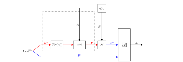
Figure 3: Coding scheme with causal CSI at the encoder, using generalized super-dense coding for the virtual channel $\mathcal{M}_{K\rightarrow B^{\prime}}$. The quantum systems of Alice and Bob are marked in red and blue, respectively. The blocks inside the dashed-line rectangle correspond to Alice’s operations.

B-A2 Encoding and Decoding

The coding scheme is depicted in Figure 3. To send a message $m\in[1:2^{nR}]$, given a parameter sequence $s^{n}\in\mathcal{S}^{n}$, Alice performs the following.

1. Apply the operator $U(\gamma(m))$ to $|\xi_{KB}\rangle^{\otimes n}$, which yields

   $$|\varphi_{K^{n}B^{n}}^{m}\rangle\equiv(U(\gamma(m)\otimes\text{1})|\xi_{KB}\rangle^{\otimes n}\,.$$ (62)

2. Then, at time $i\in[1:n]$, apply the channel $(\mathcal{F}^{(s_{i})}\otimes\text{1})$ to $|\varphi_{K_{i}B_{i}}^{m}\rangle$, and send the system $A_{i}$ through the channel.

Bob receives the systems $B^{\prime n}$ at state $\omega_{B^{\prime n}B^{n}}$ and decodes the message by applying a POVM $\{\Lambda_{m}\}_{m\in[1:2^{nR}]}$, which will be specified later.

B-A3 Code Properties

First, we write the entangled states as a combination of maximally entangled states over the typical subspaces, and then we can use the following useful identities. For a maximally entangled state $|\Phi_{AB}\rangle=\frac{1}{\sqrt{D}}\sum_{j=0}^{D-1}|j\rangle_{A}\otimes|j\rangle_{B}$,

$$\mathrm{Tr}_{B}\left(|\Phi_{AB}\rangle\langle\Phi_{AB}|\right)=\pi_{A}$$ (63)

where $\pi_{A}=\frac{1}{D}\sum_{x\in\mathcal{X}}|x\rangle\langle x|$ is the maximally mixed state. Furthermore, for every state $\rho$ of the system $A$,

$$\frac{1}{D^{2}}\sum_{a=0}^{D-1}\sum_{b=0}^{D-1}\Sigma(a,b)\,\rho\,\Sigma^{\dagger}(a,b)=\pi_{A}$$ (64)

(see e.g. [7] [67, Exercise 4.7.6])). Another useful identity is the “ricochet property” [37, Eq. (17)],

$$(U\otimes\text{1})|\Phi_{AB}\rangle=(\text{1}\otimes U^{T})|\Phi_{AB}\rangle\,.$$ (65)

Now,

$$|\xi_{K,B}\rangle^{\otimes n}= \sum_{x^{n}\in\mathcal{X}^{n}}\sqrt{p_{X^{n}}(x^{n})}|x^{n}\rangle\otimes|\psi_{x^{n}}\rangle$$ (66)

where $p_{X^{n}}(x^{n})=\prod_{i=1}^{n}p_{X}(x_{i})$ and $|\psi_{x^{n}}\rangle=|\psi_{x_{1}}\rangle\otimes|\psi_{x_{2}}\rangle\otimes\cdots\otimes|\psi_{x_{n}}\rangle$. As the space $\mathcal{X}^{n}$ can be partitioned into type classes, we may write

$$|\xi_{K,B}\rangle^{\otimes n}= \sum_{t\in\mathcal{P}_{n}(\mathcal{X})}\sum_{x^{n}\in\mathcal{T}_{n}(\hat{P})}\sqrt{p_{X^{n}}(x^{n})}|x^{n}\rangle\otimes|\psi_{x^{n}}\rangle$$

$$= \sum_{t\in\mathcal{P}_{n}(\mathcal{X})}\sqrt{p_{X^{n}}(x_{t}^{n})}\sum_{x^{n}\in\mathcal{T}_{n}(t)}|x^{n}\rangle\otimes|\psi_{x^{n}}\rangle$$ (67)

where $x_{t}^{n}$ is any sequence in the type class $\mathcal{T}_{n}(t)$. Therefore, we have that

$$|\xi_{K,B}\rangle^{\otimes n}= \sum_{t\in\mathcal{P}_{n}(\mathcal{X})}\sqrt{P(t)}|\Phi_{t}\rangle\,,$$ (68)

where

$$P(t)=d_{t}\cdot p_{X^{n}}(x_{t}^{n})\,,\;\text{with $d_{t}\equiv|\mathcal{T}_{n}(t)|$}$$

$$|\Phi_{t}\rangle=\frac{1}{\sqrt{d_{t}}}\sum_{x^{n}\in\mathcal{T}_{n}(t)}|x^{n}\rangle\otimes|\psi_{x^{n}}\rangle$$ (69)

We note that $P(t)$ is the probability of the type $\mathcal{T}_{n}(t)$ for a classical random sequence $X^{n}\sim p_{X^{n}}$.

Now, Alice applies the operator $U(\gamma(m))$ to the entangled states. Since the state $|\Phi_{t}\rangle$ is maximally entangled, we have by the “ricochet property” (65) that

$$|\varphi_{K^{n}B^{n}}^{m}\rangle\equiv(U(\gamma(m))\otimes\text{1})|\xi_{K,B}\rangle^{\otimes n}=(\text{1}\otimes U^{T}(\gamma(m)))|\xi_{K,B}\rangle^{\otimes n}\,.$$ (70)

That is, Alice’s unitary operations can be reflected and treated as if performed by Bob. Then, Alice applies the channels $\mathcal{F}^{(s_{i})}$ to her share of $|\varphi_{K_{i}B_{i}}^{m}\rangle$.

Subsequently, Bob receives the systems $B^{\prime n}$ at state

$$\rho^{\gamma(m)}_{B^{\prime n},B^{n}}= \sum_{s^{n}\in\mathcal{S}^{n}}q^{n}(s^{n})(\mathcal{N}^{(s^{n})}\otimes\text{1})(\mathcal{F}^{(s^{n})}\otimes\text{1})\left(\left(|\varphi_{K^{n}B^{n}}^{m}\rangle\langle\varphi_{K^{n}B^{n}}^{m}|\right)\right)$$ (71)

$$= (\mathcal{M}^{\otimes n}\otimes\text{1})\left((\text{1}\otimes U^{T}(\gamma(m)))(|\xi_{KB}\rangle\langle\xi_{KB}|)^{\otimes n}(\text{1}\otimes U^{*}(\gamma(m)))\right)$$ (72)

where the last line is due to (70). Since a quantum channel is a linear map, the above can be written as

$$\rho^{\gamma}_{B^{\prime n},B^{n}}= (\text{1}\otimes U^{T}(\gamma))\left[\left((\mathcal{M}\otimes\text{1})(|\xi_{KB}\rangle\langle\xi_{KB}|)\right)^{\otimes n}\right](\text{1}\otimes U^{*}(\gamma))$$

$$= (\text{1}\otimes U^{T}(\gamma))\omega_{B^{\prime}B}^{\otimes n}(\text{1}\otimes U^{*}(\gamma))$$ (73)

where we have defined

$$\omega_{B^{\prime}B}=(\mathcal{M}\otimes\text{1})(|\xi_{KB}\rangle\langle\xi_{KB}|)\,.$$ (74)

B-A4 Packing Lemma Requirements

Next, we use the quantum packing lemma. Consider the ensemble $\left\{p(\gamma)=\frac{1}{|\Gamma|},\rho^{\gamma}_{B^{\prime n},B^{n}}\right\}$, for which the expected density operator is

$$\sigma_{B^{\prime n},B^{n}}=\frac{1}{|\Gamma|}\sum_{\gamma\in\Gamma}\rho^{\gamma}_{B^{\prime n},B^{n}}\,.$$ (75)

Define the code projector and the codeword projectors by

$$\Pi\equiv \Pi^{\delta}(\omega_{B^{\prime}})\otimes\Pi^{\delta}(\omega_{B})$$ (76)

$$\Pi_{\gamma}\equiv (\text{1}\otimes U^{T}(\gamma))\Pi^{\delta}(\omega_{B^{\prime}B})(\text{1}\otimes U^{*}(\gamma))\,,\;\text{for $\gamma\in\Gamma$}$$ (77)

where $\Pi^{\delta}(\omega_{B^{\prime}B})$, $\Pi^{\delta}(\omega_{B^{\prime}})$ and $\Pi^{\delta}(\omega_{B})$ are the projectors onto the $\delta$-typical subspaces associated with the states $\omega_{B^{\prime}B}$, $\omega_{B^{\prime}}=\mathrm{Tr}_{B}(\omega_{B^{\prime}B})$ and $\omega_{B}=\mathrm{Tr}_{B^{\prime}}(\omega_{B^{\prime}B})$, respectively (see (74)). Now, we verify that the assumptions of Lemma 4 hold with respect to the ensemble and the projectors above.

First, we show that $\mathrm{Tr}(\Pi\rho^{\gamma}_{B^{\prime n},B^{n}})\geq\,1-\alpha$, where $\alpha>0$ is arbitrarilly small. Defining $\check{P}=\text{1}-P$, we have that

$$\Pi=(\text{1}-\check{\Pi}^{\delta}(\rho_{B^{\prime}}))\otimes(\text{1}-\check{\Pi}^{\delta}(\rho_{B}))\succeq(\text{1}\otimes\text{1})-(\check{\Pi}^{\delta}(\rho_{B^{\prime}})\times\text{1})-(\text{1}\otimes\check{\Pi}^{\delta}(\rho_{B}))$$ (78)

hence,

$$\mathrm{Tr}(\Pi\rho^{\gamma}_{B^{\prime n},B^{n}})\geq 1-\mathrm{Tr}\left((\check{\Pi}^{\delta}(\rho_{B^{\prime}})\otimes\text{1})\rho^{\gamma}_{B^{\prime n},B^{n}}\right)-\mathrm{Tr}\left((\text{1}\otimes\check{\Pi}^{\delta}(\rho_{B}))\rho^{\gamma}_{B^{\prime n},B^{n}}\right)$$

$$= 1-\mathrm{Tr}\left(\check{\Pi}^{\delta}(\rho_{B^{\prime}})\rho^{\gamma}_{B^{\prime n}}\right)-\mathrm{Tr}\left(\check{\Pi}^{\delta}(\rho_{B})\rho^{\gamma}_{B^{n}}\right)\,.$$ (79)

The first trace term in the RHS of (79) equals $\mathrm{Tr}\left(\check{\Pi}^{\delta}(\rho_{B^{\prime}})\omega_{B^{\prime}}^{\otimes n}\right)$ by (73), and the last term equals $\mathrm{Tr}\left(\check{\Pi}^{\delta}(\rho_{B})\omega_{B}^{\otimes n}\right)$ by (71) and (74). Therefore, we have by (24) that

$$\mathrm{Tr}(\Pi\rho^{\gamma}_{B^{\prime n},B^{n}})\geq 1-\mathrm{Tr}\left(\check{\Pi}^{\delta}(\rho_{B^{\prime}})\omega_{B^{\prime}}^{\otimes n}\right)-\mathrm{Tr}\left(\check{\Pi}^{\delta}(\rho_{B}))\omega_{B}^{\otimes n}\right)$$

$$\geq 1-2\varepsilon\,.$$ (80)

Similarly, the second requirement of the packing lemma holds since

$$\mathrm{Tr}(\Pi_{\gamma}\rho^{\gamma}_{B^{\prime n},B^{n}})= \mathrm{Tr}\left[(\text{1}\otimes U^{T}(\gamma))\Pi^{\delta}(\omega_{B^{\prime}B})(\text{1}\otimes U^{*}(\gamma))(\text{1}\otimes U^{T}(\gamma))\omega_{B^{\prime}B}^{\otimes n}(\text{1}\otimes U^{*}(\gamma))\right]$$

$$= \mathrm{Tr}(\Pi^{\delta}(\omega_{B^{\prime}B})\omega_{B^{\prime}B}^{\otimes n})\geq 1-\varepsilon$$ (81)

where the second equality follows from the cyclicity of the trace and the fact that $U^{*}U^{T}=(UU^{\dagger})^{*}=\text{1}$ for a unitary operator, and the last inequality is due to (24).

Moving to the third requirement in Lemma 4,

$$\mathrm{Tr}(\Pi_{\gamma})=\mathrm{Tr}\left((\text{1}\otimes U^{T}(\gamma))\Pi^{\delta}(\omega_{B^{\prime}B})(\text{1}\otimes U^{*}(\gamma))\right)=\mathrm{Tr}(\Pi^{\delta}(\omega_{B^{\prime}B}))\leq 2^{n(H(\omega_{B^{\prime}B})+c\delta)}$$ (82)

where the second equality holds by cyclicity of the trace and the last inequality is due to (26). It is left to verify that the last requirement of the packing lemma holds, i.e. $\Pi\sigma_{B^{\prime n},B^{n}}\Pi\preceq\,2^{-n(H(\sigma_{B^{\prime}})+H(\sigma_{B})-\alpha)}\Pi$. To this end, observe that by (72) and (75),

$$\sigma_{B^{\prime n},B^{n}}=(\mathcal{M}^{\otimes n}\otimes\text{1})\tau_{K^{n},B^{n}}$$ (83)

where we have defined

$$\tau_{K^{n},B^{n}}\equiv\frac{1}{|\Gamma|}\sum_{\gamma\in\Gamma}(\text{1}\otimes U^{T}(\gamma))(|\xi_{KB}\rangle\langle\xi_{KB}|)^{\otimes n}(\text{1}\otimes U^{*}(\gamma))\,.$$ (84)

Then, by (70) along with (60)-(61),

$$\tau_{K^{n},B^{n}}= \frac{1}{|\Gamma|}\sum_{\gamma\in\Gamma}(\text{1}\otimes U^{T}(\gamma))\left(\sum_{t}\sqrt{P(t|s^{n})}|\Phi_{t}\rangle\right)\left(\sum_{t^{\prime}}\sqrt{P(t^{\prime})}\langle\Phi_{t^{\prime}}|\right)(\text{1}\otimes U^{*}(\gamma))$$

$$= \frac{1}{|\Gamma|}\sum_{\gamma\in\Gamma}\left(\sum_{t}\sqrt{P(t)}(-1)^{c_{t}(\gamma)}(\text{1}\otimes\Sigma^{T}_{a_{t}(\gamma),b_{t}(\gamma)})|\Phi_{t}\rangle\right)$$

$$\quad\left(\sum_{t^{\prime}}\sqrt{P(t^{\prime})}(-1)^{c_{t^{\prime}}(\gamma)}\langle\Phi_{t^{\prime}}|(\text{1}\otimes\Sigma^{*}_{a_{t^{\prime}}(\gamma),b_{t^{\prime}}(\gamma)})\right)\,.$$ (85)

For $t^{\prime}=t$, the expression above becomes

$$\frac{1}{|\Gamma|}\sum_{\gamma\in\Gamma}\sum_{t}P(t)(\text{1}\otimes\Sigma^{T}_{a_{t}(\gamma),b_{t}(\gamma)})|\Phi_{t}\rangle\langle\Phi_{t}|(\text{1}\otimes\Sigma^{*}_{a_{t}(\gamma),b_{t}(\gamma)})$$

$$= \sum_{t}P(t|s^{n})\left[\frac{1}{D_{t}^{2}}\sum_{a_{t},b_{t}}(\text{1}\otimes\Sigma^{T}_{a_{t},b_{t}})|\Phi_{t}\rangle\langle\Phi_{t}|(\text{1}\otimes\Sigma^{*}_{a_{t},b_{t}})\right]=\sum_{t}P(t)\pi^{t}_{K^{n}}\times\pi^{t}_{B^{n}}$$ (86)

with

$$\pi^{t}_{K^{n}}\equiv\frac{\Pi_{K^{n}}(t)}{\mathrm{Tr}(\Pi_{K^{n}}(t))}\,,\;\pi^{t}_{B^{n}}\equiv\frac{\Pi_{B^{n}}(t)}{\mathrm{Tr}(\Pi_{B^{n}}(t))}$$ (87)

where $\Pi_{K^{n}}(t)$ is the projector of type $t$ as defined in (21). The last equality in (86) follows from (64). On the other hand, for $t^{\prime}\neq t$,

$$\frac{1}{|\Gamma|}\sum_{\gamma\in\Gamma}\sum_{t}\sum_{t^{\prime}\neq t}\sqrt{P(t)P(t^{\prime})}\frac{1}{4D_{t}^{2}D_{t^{\prime}}^{2}}\sum_{c_{t},c_{t^{\prime}}\in\{0,1\}}(-1)^{c_{t}+c_{t^{\prime}}}\sum_{a_{t},a_{t^{\prime}},b_{t},b_{t^{\prime}}}(\text{1}\otimes\Sigma^{T}_{a_{t},b_{t}})|\Phi_{t}\rangle\langle\Phi_{t^{\prime}}|(\text{1}\otimes\Sigma^{*}_{a_{t^{\prime}},b_{t^{\prime}}})=0\,.$$ (88)

We deduce from (85)-(88) that $\tau_{K^{n},B^{n}}=\sum_{t}P(t)\pi^{t}_{K^{n}}\otimes\pi^{t}_{B^{n}}$. Plugging this into (83) yields

$$\sigma_{B^{\prime n},B^{n}}=\sum_{t}P(t)\mathcal{M}^{\otimes n}(\pi^{t}_{K^{n}})\otimes\pi^{t}_{B^{n}}\,.$$ (89)

Now, we use the formula above in order to show that the last requirement in Lemma 4 holds. Consider that

$$\Pi\sigma_{B^{\prime n},B^{n}}\Pi= (\Pi^{\delta}(\omega_{B^{\prime}})\otimes\Pi^{\delta}(\omega_{B}))\sigma_{B^{\prime n},B^{n}}(\Pi^{\delta}(\omega_{B^{\prime}})\otimes\Pi^{\delta}(\omega_{B}))$$

$$= \sum_{t}P(t)\big{(}\Pi^{\delta}(\omega_{B^{\prime}})\mathcal{M}^{\otimes n}(\pi^{t}_{A^{n}})\Pi^{\delta}(\omega_{B^{\prime}})\big{)}\otimes\big{(}\Pi^{\delta}(\omega_{B})\pi^{t}_{B^{n}}\Pi^{\delta}(\omega_{B})\big{)}\,.$$ (90)

Using (87), this can be bounded by

$$\Pi\sigma_{B^{\prime n},B^{n}}\Pi= \sum_{t}P(t)\big{(}\Pi^{\delta}(\omega_{B^{\prime}})\mathcal{M}^{\otimes n}(\pi^{t}_{K^{n}})\Pi^{\delta}(\omega_{B^{\prime}})\big{)}\otimes\big{(}\Pi^{\delta}(\omega_{B})\frac{\Pi_{B^{n}}(t)}{\mathrm{Tr}(\Pi_{B^{n}}(t))}\Pi^{\delta}(\omega_{B})\big{)}$$

$$\preceq 2^{-n(H(\omega_{B})+\varepsilon_{1})}\sum_{t}P(t)\big{(}\Pi^{\delta}(\omega_{B^{\prime}})\mathcal{M}^{\otimes n}(\pi^{t}_{K^{n}})\Pi^{\delta}(\omega_{B^{\prime}})\big{)}\otimes\Pi^{\delta}(\omega_{B})$$ (91)

with arbitrarily small $\varepsilon_{1}>0$, following (22) and the fact that $\Pi^{\delta}(\omega_{B})\Pi_{B^{n}}(t)\Pi^{\delta}(\omega_{B})\preceq\Pi^{\delta}(\omega_{B})$. By linearity, this can also be written as

$$\Pi\sigma_{B^{\prime n},B^{n}}\Pi\preceq 2^{-n(H(\omega_{B})+\varepsilon_{1})}\Pi^{\delta}(\omega_{B^{\prime}})\left[\mathcal{M}^{\otimes n}\left(\sum_{t}P(t)\pi^{t}_{K^{n}}\right)\right]\Pi^{\delta}(\omega_{B^{\prime}})\otimes\Pi^{\delta}(\omega_{B})$$

$$= 2^{-n(H(\omega_{B})+\varepsilon_{1})}\Pi^{\delta}(\omega_{B^{\prime}})\left[\mathcal{M}^{\otimes n}\left(\omega_{K^{n}}\right)\right]\Pi^{\delta}(\omega_{B^{\prime}})\otimes\Pi^{\delta}(\omega_{B})$$ (92)

(see (68)). Since the expression in the square brackets equals $\omega_{B^{\prime}}^{\otimes n}$ (see (74)), we have by (25) that

$$\Pi\sigma_{B^{\prime n},B^{n}}\Pi\preceq 2^{-n(H(\omega_{B}^{\prime})+H(\omega_{B})+\varepsilon_{1}+\varepsilon_{2})}\Pi^{\delta}(\omega_{B^{\prime}})\otimes\Pi^{\delta}(\omega_{B})=2^{-n(H(\omega_{B}^{\prime})+H(\omega_{B})+\varepsilon_{1}+\varepsilon_{2})}\Pi$$ (93)

with arbitrarily small $\varepsilon_{2}>0$, where the last equality follows from the definition of $\Pi$ in (76). It follows that all of the requirements of the packing lemma are satisfied.

Hence, by Lemma 4, there exist deterministic vectors $\gamma(m)$, $m\in[1:2^{nR}]$, and a POVM $\{\Lambda_{m}\}_{m\in[1:2^{n\widetilde{R}}]}$ such that

$$\mathrm{Tr}\left(\Lambda_{m}\rho^{\gamma(m)}_{B^{\prime n},B^{n}}\right)\geq 1-2^{-n[I(B^{\prime};B)_{\omega}-R-\varepsilon^{\prime}]}$$ (94)

for all $m\in[1:2^{nR}]$, where $\varepsilon^{\prime}$ is arbitrarily small. That is, the probability of error is bounded by $2^{-n[I(B^{\prime};B)_{\omega}-R-\varepsilon_{n}(\alpha)]}$, which tends to zero if

$$R<I(B^{\prime};B)_{\omega}-\varepsilon^{\prime}\,.$$ (95)

Now, consider the systems $S,K_{1},A_{1},A_{1}^{\prime},B_{1}$ at state

$$\omega^{s}_{A_{1}A_{1}^{\prime}}=(\mathcal{F}_{1}^{(s)}\otimes\text{1})(|\xi_{K_{1},A_{1}^{\prime}}\rangle\langle\xi_{K_{1},A_{1}^{\prime}}|)$$ (96)

$$\omega_{A_{1}SA_{1}^{\prime}}=\sum_{s\in\mathcal{S}}q(s)|s\rangle\langle s|\otimes\omega^{s}_{A_{1}A_{1}^{\prime}}$$ (97)

$$\omega_{A_{1}B_{1}}=(\text{1}\otimes\mathcal{N})(\omega_{A_{1}SA_{1}^{\prime}})=(\text{1}\otimes\mathcal{M})(|\xi_{K_{1},A_{1}^{\prime}}\rangle\langle\xi_{K_{1},A_{1}^{\prime}}|)\,.$$ (98)

Observe that this is the same relation as in (74) where $A_{1}^{\prime}$, $K_{1}$ and $B_{1}$ take place with $A$, $B$, and $B^{\prime}$, respectively, where $\mathcal{F}_{1}^{(s)}$ is defined with Kraus operators $F_{1,j}^{(s)}\equiv(F_{j}^{(s)})^{T}$ for $s\in\mathcal{S}$, due to (68) and the “ricochet property” (65). Thus, the probability of error tends to zero as $n\rightarrow\infty$ provided that $R<I(K_{1};B_{1})_{\omega}-\varepsilon^{\prime}$. This completes the proof of the direct part.

B-B Converse Proof

Consider the converse part. Suppose that Alice and Bob are trying to distribute randomness. An upper bound on the rate at which Alice can distribute randomness to Bob also serves as an upper bound on the rate at which they can communicate. In this task, Alice and Bob share an entangled state $\Psi^{\otimes n}_{T_{A}T_{B}}$. Alice first prepares the maximally corrleated state

$$\overline{\Phi}_{MM^{\prime}}\equiv\frac{1}{2^{nR}}\sum_{m=1}^{2^{nR}}|m\rangle\langle m|\otimes|\phi_{m}\rangle\langle\phi_{m}|\,.$$ (99)

locally. We note that since $M$ and $M^{\prime}$ are classical, they can be copied.

Then, at time $i\in[1:n]$, Alice applies an encoding channel $\mathcal{E}^{s^{i}}_{M^{\prime}T_{Ai}\rightarrow A_{i}^{\prime}}$ to the classical system $M^{\prime}$ and her share $T_{Ai}$ of the entangled state $\Psi^{\otimes n}_{T_{A}T_{B}}$. The resulting state is $\omega_{S^{i}MA^{\prime}_{i}T_{Bi}}=\sum_{s^{i}\in\mathcal{S}^{i}}q^{i}(s^{i})|s^{i}\rangle\langle s^{i}|\otimes\rho^{s^{i}}_{MA^{\prime}_{i}T_{Bi}}$, with

$$\rho^{s^{i}}_{MA^{\prime}_{i}T_{Bi}}\equiv(\text{1}\otimes\mathcal{E}^{s^{i}}\otimes\text{1})(\overline{\Phi}_{MM^{\prime}}\otimes\Psi_{T_{Ai}T_{Bi}})\,,$$ (100)

for $i\in[1:n]$. After Alice sends the systems $A^{\prime n}$ through the channel, Bob receives the systems $B^{n}$ at state $\omega_{S^{n}MB^{n}T_{B}^{n}}=\sum_{s^{n}\in\mathcal{S}^{n}}q^{n}(s^{n})|s^{n}\rangle\langle s^{n}|\otimes\rho^{s_{1}}_{MB_{1}T_{B1}}\otimes\rho^{s_{1},s_{2}}_{MB_{2}T_{B2}}\otimes\cdots\otimes\rho^{s^{n}}_{MB_{n}T_{Bn}}$, with

$$\rho^{s^{i}}_{MB_{i}T_{Bi}}\equiv(\text{1}\otimes\mathcal{N}^{(s_{i})}\otimes\text{1})(\rho^{s^{i}}_{MA^{\prime}_{i}T_{Bi}})\,,$$ (101)

for $i\in[1:n]$. Then, Bob performs a decoding channel $\mathcal{D}_{B^{n}T_{B}^{n}\rightarrow\hat{M}}$, producing $\omega_{S^{n}M\hat{M}}^{\prime}=\sum_{s^{n}\in\mathcal{S}^{n}}q^{n}(s^{n})|s^{n}\rangle\langle s^{n}|\otimes\rho^{s^{n}}_{M\hat{M}}$ with

$$\rho^{s^{n}}_{M\hat{M}}\equiv(\text{1}\otimes\mathcal{D})\left(\bigotimes_{i=1}^{n}\rho^{s^{i}}_{MB_{i}T_{Bi}}\right)$$ (102)

Consider a sequence of codes $(\mathcal{E}_{n}^{s^{i}},\Psi_{n},\mathcal{D}_{n})$ for randomness distribution, such that

$$\frac{1}{2}\left\lVert\omega_{M\hat{M}}-\overline{\Phi}_{MM^{\prime}}\right\rVert_{1}\leq\alpha_{n}\,,$$ (103)

where $\omega_{M\hat{M}}$ is the reduced density operator of $\omega_{S^{n}M\hat{M}}$ and while $\alpha_{n}$ tends to zero as $n\rightarrow\infty$. By the Alicki-Fannes-Winter inequality [1, 69] [67, Theorem 11.10.3], this implies that

$$|H(M|\hat{M})_{\omega}-H(M|M^{\prime})_{\overline{\Phi}}|\leq n\varepsilon_{n}$$ (104)

while $\varepsilon_{n}$ tends to zero as $n\rightarrow\infty$. Now, observe that $H(\overline{\Phi}_{MM^{\prime}})=H(\overline{\Phi}_{M})=H(\overline{\Phi}_{M^{\prime}})=nR$, hence $I(M;\hat{M})_{\overline{\Phi}}=nR$. Also, $H(\omega_{M})=H(\overline{\Phi}_{M})=nR$ implies that $I(M;M^{\prime})_{\overline{\Phi}}-I(M;\hat{M})_{\omega}=H(M|\hat{M})_{\omega}-H(M|M^{\prime})_{\overline{\Phi}}$. Therefore, by (104),

$$nR= I(M;\hat{M})_{\overline{\Phi}}$$

$$\leq I(M;\hat{M})_{\omega}+n\varepsilon_{n}$$

$$\leq I(M;T_{B},B^{n})_{\omega}+n\varepsilon_{n}$$ (105)

where the last line follows from (102) and the quantum data processing inequality [53, Theorem 11.5].

As in the classical case, the chain rule for the quantum mutual information states that $I(A;B,C)_{\sigma}=I(A;B)_{\sigma}+I(A;C|B)_{\sigma}$ for all $\sigma_{ABC}$ (see e.g. [67, Property 11.7.1]). Hence,

$$nR\leq I(T_{B},M;B^{n})_{\omega}+I(M;T_{B})_{\omega}-I(T_{B};B^{n})_{\omega}+n\varepsilon_{n}$$

$$\leq I(T_{B},M;B^{n})_{\omega}+I(M;T_{B})_{\omega}+n\varepsilon_{n}$$

$$= I(T_{B},M;B^{n})_{\omega}+n\varepsilon_{n}$$ (106)

where the equality holds since the systems $M$ and $T_{B}$ are in a product state. The chain rule further implies that

$$I(T_{B},M;B^{n})_{\omega}= \sum_{i=1}^{n}I(T_{B},M;B_{i}|B^{i-1})_{\omega}$$

$$\leq \sum_{i=1}^{n}I(T_{B},M,S^{i-1},A^{\prime i-1},B^{i-1};B_{i})_{\omega}$$

$$= \sum_{i=1}^{n}[I(T_{B},M,S^{i-1},A^{\prime i-1};B_{i})_{\omega}+I(B^{i-1};B_{i}|T_{B},M,S^{i-1},A^{i-1})_{\omega}]$$

$$= \sum_{i=1}^{n}I(T_{B},M,S^{i-1},A^{\prime i-1};B_{i})_{\omega}$$ (107)

where the last line holds since the channel has a product form, i.e. $\mathcal{N}_{S^{i}A^{\prime i}\rightarrow B^{i}}=\mathcal{N}^{\otimes i}=\mathcal{N}_{S^{i-1}A^{\prime i-1}\rightarrow B^{i-1}}\otimes\mathcal{N}_{S_{i}A_{i}^{\prime}\rightarrow B_{i}}$. Defining $K_{i}=(M,M^{\prime},S^{i-1},A^{\prime i-1},T_{A},T_{B})$ and a quantum channel $\mathcal{F}^{(s_{i})}_{K_{i}\rightarrow A_{i}}$, we have by (106) and (107) that

$$R-\varepsilon_{n}\leq\frac{1}{n}\sum_{i=1}^{n}I(K_{i};B_{i})_{\omega}\leq\max_{\theta_{KA^{\prime}}\,,\;\mathcal{F}^{(s)}_{K\rightarrow A}}I(K;B)_{\omega}\,.$$ (108)

Observe that by (100), $K_{i}$ and $S_{i}$ are in a product state as required. This concludes the proof of Theorem 6. ∎

Appendix C Proof of Lemma 8

Fix the quantum state $\theta_{KA^{\prime}}$ and channels $\mathcal{F}^{(s)}_{K\rightarrow A}$, $s\in\mathcal{S}$, such that

$$\mathsf{C}_{E,\text{n-c}}(\mathcal{N})=I(A;B)_{\omega}-I(A;S)_{\omega}$$ (109)

and consider the spectral decomposition,

$$\theta_{KA^{\prime}}=\sum_{x\in\mathcal{X}}\sum_{z\in\mathcal{Z}}p_{X,Z}(x,z)|x\rangle\langle x|\otimes|z\rangle\langle z|$$ (110)

where $P_{X,Z}(x,z)$ is a probability distribution, while $\{|x\rangle\}_{x\in\mathcal{X}}$ and $\{|z\rangle\}_{z\in\mathcal{Z}}$ are orthonormal bases of the Hilbert spaces $\mathcal{H}_{K}$ and $\mathcal{H}_{A^{\prime}}$, respectively. Also, for every $s\in\mathcal{S}$, consider the Kraus representation of each channel

$$\mathcal{F}^{(s)}_{K\rightarrow A}(\rho_{K})=\sum_{j}F_{j}^{(s)}\rho_{A}F_{j}^{(s)\,\dagger}$$ (111)

with $\sum_{j}F_{j}^{(s)\,\dagger}F_{j}^{(s)}=\text{1}$ (see Subsection II-B).

First, we show that maximizing over pure states is sufficient. To this end, we perform purification of the state $\theta_{KA^{\prime}}$. Specifically, define the pure state

$$|\xi_{KJA^{\prime}}\rangle=\sum_{x\in\mathcal{X}}\sum_{z\in\mathcal{Z}}\sqrt{p_{X,Z}(x,z)}|x\rangle\otimes|\psi_{x}\rangle\otimes|z\rangle$$ (112)

where $J$ is a reference system and $|\psi_{x}\rangle$ are orthonormal vectors in $\mathcal{H}_{J}$. Observe that $|\xi_{KJA^{\prime}}\rangle$ is a purification of the mixed state $\theta_{KA^{\prime}}$, namely, $\theta_{KA^{\prime}}=\mathrm{Tr}_{J}(||\xi_{KJA^{\prime}}\rangle\rangle\langle|\xi_{KJA^{\prime}}\rangle|)$. Defining $\widetilde{\mathcal{F}}^{(s)}_{KJ\rightarrow A}=(\mathcal{F}^{(s)}_{K\rightarrow A}\otimes\text{1})$ and $\widetilde{K}=(K,J)$, we have that

$$\omega_{AA^{\prime}}=\widetilde{\mathcal{F}}^{(s)}_{\widetilde{K}\rightarrow A}(|\xi_{\widetilde{K}A^{\prime}}\rangle\langle\xi_{\widetilde{K}A^{\prime}}|)\,.$$ (113)

Then, observe that the mutual information difference $[I(A;B)_{\omega}-I(A;S)_{\omega}]$ depends on the state $\theta_{KA^{\prime}}$ and the channels $\mathcal{F}^{(s)}_{K\rightarrow A}$ only through $\omega_{AA^{\prime}}$, and thus, $\theta_{KA^{\prime}}$ can be replaced by the pure state $|\xi_{\widetilde{K}A^{\prime}}\rangle$.

To show that maximizing over isometric channels is sufficient, we use an isometric extension of the channels $\mathcal{F}_{K\rightarrow A}^{(s)}$, for $s\in\mathcal{S}$. Define the isometric channels $\overline{\mathcal{F}}_{K\rightarrow AE}^{(s)}$ by

$$\overline{\mathcal{F}}^{(s)}_{K\rightarrow AE}(\rho_{K})=\overline{F}^{(s)}\rho_{K}\overline{F}^{(s)\,\dagger}$$ (114a)

for all $$\rho_{K}$$, with

$$\overline{F}^{(s)}=\sum_{j}F_{j}^{(s)}\otimes|j\rangle$$ (114b)

where $E$ is a reference system and $\{|j\rangle\}$ is an orthonormal basis of $\mathcal{H}_{E}$. Observe that $\overline{\mathcal{F}}^{(s)}_{K\rightarrow AE}$ is an extension of the quantum channel $\mathcal{F}^{(s)}_{K\rightarrow A}$, namely, $\mathrm{Tr}_{E}\left(\overline{\mathcal{F}}^{(s)}_{K\rightarrow AE}(\rho_{K})\right)=\mathcal{F}^{(s)}_{K\rightarrow A}(\rho_{K})$ for every $\rho_{K}$.

Let

$$\sigma^{s}_{AEA^{\prime}}=(\overline{\mathcal{F}}^{(s)}_{K\rightarrow AE}\otimes\text{1})(\theta_{KA^{\prime}})$$ (115)

$$\sigma_{AESA^{\prime}}=\sum_{s\in\mathcal{S}}q(s)|s\rangle\langle s|\otimes\sigma^{s}_{AEA^{\prime}}$$ (116)

$$\sigma_{AEB}=(\text{1}\otimes\text{1}\otimes\mathcal{N})(\sigma_{AESA^{\prime}})\,.$$ (117)

Based on the definition in (40),

$$\mathsf{C}_{E,\text{n-c}}(\mathcal{N})\geq I(A,E;B)_{\sigma}-I(A,E;S)_{\sigma}\,.$$ (118)

On the other hand, by the quantum data processing theorem due to Schumacher and Nielsen [56][67, Theorem 11.9.4],

$$I(A;B)_{\omega}\leq I(A,E;B)_{\sigma}\,.$$ (119)

Furthermore, by (114), the systems $S$ and $E$ are in a product state given $A$, hence $I(E;S|A)_{\sigma}=0$. Thus,

$$I(A;S)_{\omega}=I(A;S)_{\sigma}=I(A;S)_{\sigma}+I(E;S|A)_{\sigma}=I(A,E;S)_{\sigma}$$ (120)

where the last equality is due to the chain rule for the quantum mutual information [67, Theorem 11.7.1]. Together, (119) and (120) imply that

$$\mathsf{C}_{E,\text{n-c}}(\mathcal{N})\leq I(A,E;B)_{\sigma}-I(A,E;S)_{\sigma}\,.$$ (121)

It thus follows that the channel $\mathcal{F}_{K\rightarrow A}^{(s)}$ in (40) can be replaced by its isometric extension $\overline{\mathcal{F}}^{(s)}_{K\rightarrow A_{0}}$, with $A_{0}=(A,E)$, for $s\in\mathcal{S}$. This completes the proof of the lemma. ∎

Appendix D Proof of Theorem 9

D-A Achievability Proof

We show that for every $\varepsilon_{0},\delta_{0}>0$, there exists a $(2^{nR},n,\varepsilon_{0})$ code for the random-parameter quantum channel $\mathcal{N}_{SA\rightarrow B}$ with non-causal CSI, provided that $R<\mathsf{C}_{E,\text{n-c}}(\mathcal{N})-\delta_{0}$. Based on Lemma 8, it suffices to consider a pure entangled state and isometric channels. Hence, let $|\xi_{AB}\rangle$ be a pure entangled state, and $\mathcal{F}^{(s)}_{K\rightarrow A}(\rho_{K})=F^{(s)}\rho_{K}F^{(s)\,\dagger}$, $s\in\mathcal{S}$, be a set of isometric channels. Suppose that Alice and Bob share the joint state $|\xi_{AB}\rangle^{\otimes n}$. Define

$$|\varphi^{s}_{AB}\rangle= (F^{(s)}\otimes\text{1})|\xi_{AB}\rangle$$ (122)

and consider the Schmidt decomposition of the state,

$$|\varphi_{A,B}^{s}\rangle=\sum_{x\in\mathcal{X}}\sqrt{p_{X|S}(x|s)}|x\rangle\otimes|\psi_{x,s}\rangle$$ (123)

where $p_{X|S}$ is a conditional probability distribution, $\{|x\rangle\}$ is an orthonormal basis of $\mathcal{H}_{A}$, and $|\psi_{x,s}\rangle$ are orthonormal vectors in $\mathcal{H}_{B}$. Observe that the quantum entropy of the system $B$ is the same as the Shannon entropy of the classical random variable $X$, i.e. $H(\omega_{SB})=H(S,X)$ and $H(\omega_{B})=H(X)$. Thus,

$$I(B;S)_{\varphi}= I(X;S)\,.$$ (124)

The code construction, encoding and decoding procedures are described below.

D-A1 Code Construction

Encoding is performed in two stages, first classical compression of the parameter sequence $S^{n}$, and then, application of quantum operators depending on the result in the first stage. The code construction is specified below.

1. Classical Compression: Let $\widetilde{R}>R$. We construct $2^{nR}$ sub-codebooks at random. For every message $m\in[1:2^{nR}]$, choose $2^{n(\widetilde{R}-R)}$ independent sequences $x^{n}(\ell)$ at random, each according to $\prod_{i=1}^{n}p_{X}(x_{i})$. Then, we have the following sub-codebooks,

   $$\mathscr{B}(m)=\{x^{n}(\ell)\,:\;\ell\in[(m-1)2^{n(\widetilde{R}-R)}+1:m2^{n(\widetilde{R}-R)}]\}\,,\;\text{for $m\in[1:2^{nR}]$}\,.$$ (125)

2. Quantum Operators: Consider the Heisenberg-Weyl operators $\{\Sigma(a,b)=X(a)Z(b)\}$ of dimension $D$, given by

   $$X(a)= \sum_{j=0}^{D-1}|a\oplus j\rangle\langle j|$$ (126)

   $$Z(b)= \sum_{j=0}^{D-1}e^{2\pi ibj/D}|j\rangle\langle j|$$ (127)

   for $a,b\in\{0,1,\ldots,D-1\}$, where $a\oplus j=(a+j)\mod D\;$ and $i=\sqrt{-1}$. For every $s^{n}\in\mathcal{S}^{n}$ and every conditional type class $\mathcal{T}_{n}(t|s^{n})$ in $\mathcal{X}^{n}$, define the operators

   $$V_{t}(a_{t},b_{t},c_{t})=(-1)^{c_{t}}\Sigma(a_{t},b_{t})\,,\;a_{t},b_{t}\in\{0,1,\ldots,D_{t}-1\}\,,\;c_{t}\in\{0,1\}$$ (128)

   where $D_{t}=|\mathcal{T}_{n}(t|s^{n})|$ is the size of type class associated with the conditional type $t$. Then, define the operator

   $$U(\gamma)=\bigoplus_{t}\,V_{t}(a_{t},b_{t},c_{t})$$ (129)

   with $\gamma=\left((a_{t},b_{t},c_{t})_{t}\right)$. Let $\Gamma$ denote the set of all possible vectors $\gamma$. Then, choose $2^{n\widetilde{R}}$ vectors $\gamma(\ell)$, $\ell\in[1:2^{n\widetilde{R}}]$, uniformly at random.

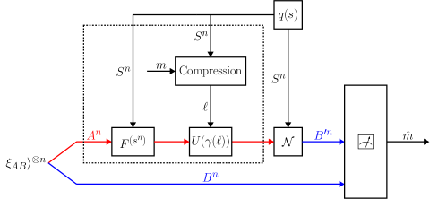
Figure 4: Coding scheme combining classical compression and generalized super-dense coding. The quantum systems of Alice and Bob are marked in red and blue, respectively. The blocks inside the dashed-line rectangle correspond to Alice’s operations.

D-A2 Encoding and Decoding

The coding scheme is depicted in Figure 4. To send a message $m\in[1:2^{nR}]$, given a parameter sequence $s^{n}\in\mathcal{S}^{n}$, Alice performs the following.

1. Find a sequence $x^{n}(\ell)\in\mathscr{B}(m)$ that is jointly typical with the parameter sequence, i.e. $(s^{n},x^{n}(\ell))\in\mathcal{A}^{\delta}(p_{S,X})$. If there is none, choose an arbitrary $\ell$.

2. Apply the operators $F^{(s_{1})},F^{(s_{2})},\ldots,F^{(s_{n})}$, and $U(\gamma(\ell))$, which yields

   $$|\varphi_{A^{n}B^{n}}^{\ell,s^{n}}\rangle\equiv(U(\gamma(\ell)F^{(s^{n})}\otimes\text{1})|\xi_{AB}\rangle^{\otimes n}=(U(\gamma(\ell)\otimes\text{1})|\varphi^{s^{n}}_{A^{n}B^{n}}\rangle$$ (130)

   with $F^{(s^{n})}\equiv F^{(s_{1})}\otimes\cdots\otimes F^{(s_{n})}$ and $|\varphi^{s^{n}}_{A^{n}B^{n}}\rangle\equiv|\varphi^{s_{1}}_{AB}\rangle\otimes\cdots\otimes|\varphi^{s_{n}}_{AB}\rangle$ (see (122)).

3. Send the systems $A^{n}$ through the channel.

Bob receives the systems $B^{\prime n}$ at state $\omega_{B^{\prime n}B^{n}}$ and applies a POVM $\{\Lambda_{\ell}\}_{\ell\in[1:2^{n\widetilde{R}}]}$, which will be specified later. Once Bob has a measurement result $\hat{\ell}$, he decodes the message as the corresponding sub-codebook. That is, Bob declares the message to be $\hat{m}\in[1:2^{nR}]$ such that $x^{n}(\hat{\ell})\in\mathscr{B}(\hat{m})$.

D-A3 Code Properties

First, we write the entangled states as a combination of maximally entangled states over the typical subspaces, and then we can use the following useful identities. For a maximally entangled state $|\Phi_{AB}\rangle=\frac{1}{\sqrt{D}}\sum_{j=0}^{D-1}|j\rangle_{A}\otimes|j\rangle_{B}$,

$$\mathrm{Tr}_{B}\left(|\Phi_{AB}\rangle\langle\Phi_{AB}|\right)=\pi_{A}$$ (131)

where $\pi_{A}=\frac{1}{D}\sum_{x\in\mathcal{X}}|x\rangle\langle x|$ is the maximally mixed state. Furthermore, for every state $\rho$ of the system $A$,

$$\frac{1}{D^{2}}\sum_{a=0}^{D-1}\sum_{b=0}^{D-1}\Sigma(a,b)\,\rho\,\Sigma^{\dagger}(a,b)=\pi_{A}$$ (132)

(see e.g. [7] [67, Exercise 4.7.6])). Another useful identity is the “ricochet property” [37, Eq. (17)],

$$(U\otimes\text{1})|\Phi_{AB}\rangle=(\text{1}\otimes U^{T})|\Phi_{AB}\rangle\,.$$ (133)

Now, for every $s^{n}\in\mathcal{S}^{n}$,

$$|\varphi^{s^{n}}_{A^{n},B^{n}}\rangle= \sum_{x^{n}\in\mathcal{X}^{n}}\sqrt{p_{X^{n}|S^{n}}(x^{n}|s^{n})}|x^{n}\rangle\otimes|\psi_{x^{n},s^{n}}\rangle$$ (134)

where $p_{X^{n}|S^{n}}(x^{n}|s^{n})=\prod_{i=1}^{n}p_{X|S}(x_{i}|s_{i})$ and $|\psi_{x^{n}}\rangle=|\psi_{x_{1}}\rangle\otimes|\psi_{x_{2}}\rangle\otimes\cdots\otimes|\psi_{x_{n}}\rangle$. As the space $\mathcal{X}^{n}$ can be partitioned into conditional type classes given $s^{n}$, we may write

$$|\varphi^{s^{n}}_{A^{n},B^{n}}\rangle= \sum_{t\in\mathcal{P}_{n}(\mathcal{X})}\sum_{x^{n}\in\mathcal{T}_{n}(\hat{P}|s^{n})}\sqrt{p_{X^{n}|S^{n}}(x^{n}|s^{n})}|x^{n}\rangle\otimes|\psi_{x^{n},s^{n}}\rangle$$

$$= \sum_{t\in\mathcal{P}_{n}(\mathcal{X})}\sqrt{p_{X^{n}|S^{n}}(x_{t}^{n}|s^{n})}\sum_{x^{n}\in\mathcal{T}_{n}(t|s^{n})}|x^{n}\rangle\otimes|\psi_{x^{n},s^{n}}\rangle$$ (135)

where $x_{t}^{n}$ is any sequence in the conditional type class $\mathcal{T}_{n}(t|s^{n})$. Therefore, we have that

$$|\varphi^{s^{n}}_{A^{n},B^{n}}\rangle= \sum_{t\in\mathcal{P}_{n}(\mathcal{X})}\sqrt{P(t|s^{n})}|\Phi_{t}\rangle\,,$$ (136)

where

$$P(t|s^{n})=d_{t}(s^{n})\cdot p_{X^{n}|S^{n}}(x_{t}^{n}|s^{n})\,,\;\text{with $d_{t}(s^{n})\equiv|\mathcal{T}_{n}(t|s^{n})|$}$$

$$|\Phi_{t}\rangle=\frac{1}{\sqrt{d_{t}(s^{n})}}\sum_{x^{n}\in\mathcal{T}_{n}(t|s^{n})}|x^{n}\rangle\otimes|\psi_{x^{n},s^{n}}\rangle$$ (137)

We note that $P(t|s^{n})$ is the conditional probability of the type $\mathcal{T}_{n}(t|s^{n})$ for a classical random sequence $X^{n}\sim p_{X^{n}|S^{n}=s^{n}}$.

Now, Alice applies the operator $U(\gamma(\ell))$ to the entangled states. Since the state $|\Phi_{t}\rangle$ is maximally entangled, we have by the “ricochet property” (133) that

$$|\varphi_{A^{n}B^{n}}^{\gamma(\ell),s^{n}}\rangle\equiv(U(\gamma(\ell))\otimes\text{1})|\varphi^{s^{n}}_{A^{n},B^{n}}\rangle=(\text{1}\otimes U^{T}(\gamma(\ell)))|\varphi^{s^{n}}_{A^{n},B^{n}}\rangle\,.$$ (138)

By the same considerations, we also have that

$$|\varphi^{s^{n}}_{A^{n},B^{n}}\rangle=(F^{(s^{n})}\otimes\text{1})|\xi_{AB}\rangle^{\otimes n}=(\text{1}\otimes(F^{(s^{n})})^{T})|\xi_{AB}\rangle^{\otimes n}\,.$$ (139)

That is, Alice’s unitary operations can be reflected and treated as if performed by Bob.

Bob then receives the systems $B^{\prime n}$ at state

$$\rho^{\gamma(\ell)}_{B^{\prime n},B^{n}}= \sum_{s^{n}\in\mathcal{S}^{n}}q^{n}(s^{n})(\mathcal{N}^{(s^{n})}\otimes\text{1})\left(\left(|\varphi_{A^{n}B^{n}}^{\gamma(\ell),s^{n}}\rangle\langle\varphi_{A^{n}B^{n}}^{\gamma(\ell),s^{n}}|\right)\right)$$ (140)

$$= \sum_{s^{n}\in\mathcal{S}^{n}}q^{n}(s^{n})(\mathcal{N}^{(s^{n})}\otimes\text{1})\left((\text{1}\otimes U^{T}(\gamma(\ell)))|\varphi_{A^{n}B^{n}}^{s^{n}}\rangle\langle\varphi_{A^{n}B^{n}}^{s^{n}}|(\text{1}\otimes U^{*}(\gamma(\ell)))\right)$$ (141)

where the last line is due to (138). Since a quantum channel is a linear map, the above can be written as

$$\rho^{\gamma}_{B^{\prime n},B^{n}}= (\text{1}\otimes U^{T}(\gamma))\left[\sum_{s^{n}\in\mathcal{S}^{n}}q^{n}(s^{n})(\mathcal{N}^{(s^{n})}\otimes\text{1})\left(|\varphi_{A^{n}B^{n}}^{s^{n}}\rangle\langle\varphi_{A^{n}B^{n}}^{s^{n}}|\right)\right](\text{1}\otimes U^{*}(\gamma))$$

$$= (\text{1}\otimes U^{T}(\gamma))\omega_{B^{\prime}B}^{\otimes n}(\text{1}\otimes U^{*}(\gamma))$$ (142)

where we have defined

$$\omega_{AB}^{s}=(\text{1}\otimes(F^{(s)})^{T})|\xi_{AB}\rangle\langle\xi_{AB}|(\text{1}\otimes(F^{(s)})^{*})$$ (143)

$$\omega_{SAB}=\sum_{s\in\mathcal{S}}q(s)|s\rangle\langle s|\otimes\omega_{AB}^{s}$$ (144)

$$\omega_{B^{\prime}B}=(\mathcal{N}\otimes\text{1})(\omega_{SAB})\,.$$ (145)

D-A4 Packing Lemma Requirements

Next, we use the quantum packing lemma. Consider the ensemble $\left\{p(\gamma)=\frac{1}{|\Gamma|},\rho^{\gamma}_{B^{\prime n},B^{n}}\right\}$, for which the expected density operator is

$$\sigma_{B^{\prime n},B^{n}}=\frac{1}{|\Gamma|}\sum_{\gamma\in\Gamma}\rho^{\gamma}_{B^{\prime n},B^{n}}\,.$$ (146)

Define the code projector and the codeword projectors by

$$\Pi\equiv \Pi^{\delta}(\omega_{B^{\prime}})\otimes\Pi^{\delta}(\omega_{B})$$ (147)

$$\Pi_{\gamma}\equiv (\text{1}\otimes U^{T}(\gamma))\Pi^{\delta}(\omega_{B^{\prime}B})(\text{1}\otimes U^{*}(\gamma))\,,\;\text{for $\gamma\in\Gamma$}$$ (148)

where $\Pi^{\delta}(\omega_{B^{\prime}B})$, $\Pi^{\delta}(\omega_{B^{\prime}})$ and $\Pi^{\delta}(\omega_{B})$ are the projectors onto the $\delta$-typical subspaces associated with the states $\omega_{B^{\prime}B}$, $\omega_{B^{\prime}}=\mathrm{Tr}_{B}(\omega_{B^{\prime}B})$ and $\omega_{B}=\mathrm{Tr}_{B^{\prime}}(\omega_{B^{\prime}B})$, respectively (see (145)). Now, we verify that the assumptions of Lemma 4 hold with respect to the ensemble and the projectors above.

First, we show that $\mathrm{Tr}(\Pi\rho^{\gamma}_{B^{\prime n},B^{n}})\geq\,1-\alpha$, where $\alpha>0$ is arbitrarilly small. Defining $\check{P}=\text{1}-P$, we have that

$$\Pi=(\text{1}-\check{\Pi}^{\delta}(\rho_{B^{\prime}}))\otimes(\text{1}-\check{\Pi}^{\delta}(\rho_{B}))\succeq(\text{1}\otimes\text{1})-(\check{\Pi}^{\delta}(\rho_{B^{\prime}})\times\text{1})-(\text{1}\otimes\check{\Pi}^{\delta}(\rho_{B}))$$ (149)

hence,

$$\mathrm{Tr}(\Pi\rho^{\gamma}_{B^{\prime n},B^{n}})\geq 1-\mathrm{Tr}\left((\check{\Pi}^{\delta}(\rho_{B^{\prime}})\otimes\text{1})\rho^{\gamma}_{B^{\prime n},B^{n}}\right)-\mathrm{Tr}\left((\text{1}\otimes\check{\Pi}^{\delta}(\rho_{B}))\rho^{\gamma}_{B^{\prime n},B^{n}}\right)$$

$$= 1-\mathrm{Tr}\left(\check{\Pi}^{\delta}(\rho_{B^{\prime}})\rho^{\gamma}_{B^{\prime n}}\right)-\mathrm{Tr}\left(\check{\Pi}^{\delta}(\rho_{B})\rho^{\gamma}_{B^{n}}\right)\,.$$ (150)

The first trace term in the RHS of (150) equals $\mathrm{Tr}\left(\check{\Pi}^{\delta}(\rho_{B^{\prime}})\omega_{B^{\prime}}^{\otimes n}\right)$ by (142), and the last term equals $\mathrm{Tr}\left(\check{\Pi}^{\delta}(\rho_{B})\omega_{B}^{\otimes n}\right)$ by (140) and (144). Therefore, we have by (24) that

$$\mathrm{Tr}(\Pi\rho^{\gamma}_{B^{\prime n},B^{n}})\geq 1-\mathrm{Tr}\left(\check{\Pi}^{\delta}(\rho_{B^{\prime}})\omega_{B^{\prime}}^{\otimes n}\right)-\mathrm{Tr}\left(\check{\Pi}^{\delta}(\rho_{B}))\omega_{B}^{\otimes n}\right)$$

$$\geq 1-2\varepsilon\,.$$ (151)

Similarly, the second requirement of the packing lemma holds since

$$\mathrm{Tr}(\Pi_{\gamma}\rho^{\gamma}_{B^{\prime n},B^{n}})= \mathrm{Tr}\left[(\text{1}\otimes U^{T}(\gamma))\Pi^{\delta}(\omega_{B^{\prime}B})(\text{1}\otimes U^{*}(\gamma))(\text{1}\otimes U^{T}(\gamma))\omega_{B^{\prime}B}^{\otimes n}(\text{1}\otimes U^{*}(\gamma))\right]$$

$$= \mathrm{Tr}(\Pi^{\delta}(\omega_{B^{\prime}B})\omega_{B^{\prime}B}^{\otimes n})\geq 1-\varepsilon$$ (152)

where the second equality follows from the cyclicity of the trace and the fact that $U^{*}U^{T}=(UU^{\dagger})^{*}=\text{1}$ for a unitary operator, and the last inequality is due to (24).

Moving to the third requirement in Lemma 4,

$$\mathrm{Tr}(\Pi_{\gamma})=\mathrm{Tr}\left((\text{1}\otimes U^{T}(\gamma))\Pi^{\delta}(\omega_{B^{\prime}B})(\text{1}\otimes U^{*}(\gamma))\right)=\mathrm{Tr}(\Pi^{\delta}(\omega_{B^{\prime}B}))\leq 2^{n(H(\omega_{B^{\prime}B})+c\delta)}$$ (153)

where the second equality holds by cyclicity of the trace and the last inequality is due to (26). It is left to verify that the last requirement of the packing lemma holds, i.e. $\Pi\sigma_{B^{\prime n},B^{n}}\Pi\preceq\,2^{-n(H(\sigma_{B^{\prime}})+H(\sigma_{B})-\alpha)}\Pi$. To this end, observe that by (141) and (146),

$$\sigma_{B^{\prime n},B^{n}}=\sum_{s^{n}\in\mathcal{S}^{n}}q^{n}(s^{n})(\mathcal{N}^{(s^{n})}\otimes\text{1})\tau^{s^{n}}_{A^{n},B^{n}}$$ (154)

where we have defined

$$\tau^{s^{n}}_{A^{n},B^{n}}\equiv\frac{1}{|\Gamma|}\sum_{\gamma\in\Gamma}(\text{1}\otimes U^{T}(\gamma))|\varphi_{A^{n}B^{n}}^{s^{n}}\rangle\langle\varphi_{A^{n}B^{n}}^{s^{n}}|(\text{1}\otimes U^{*}(\gamma))\,.$$ (155)

Then, by (138) along with (128)-(129),

$$\tau^{s^{n}}_{A^{n},B^{n}}= \frac{1}{|\Gamma|}\sum_{\gamma\in\Gamma}(\text{1}\otimes U^{T}(\gamma))\left(\sum_{t}\sqrt{P(t|s^{n})}|\Phi_{t}\rangle\right)\left(\sum_{t^{\prime}}\sqrt{P(t^{\prime}|s^{n})}\langle\Phi_{t^{\prime}}|\right)(\text{1}\otimes U^{*}(\gamma))$$

$$= \frac{1}{|\Gamma|}\sum_{\gamma\in\Gamma}\left(\sum_{t}\sqrt{P(t|s^{n})}(-1)^{c_{t}(\gamma)}(\text{1}\otimes\Sigma^{T}_{a_{t}(\gamma),b_{t}(\gamma)})|\Phi_{t}\rangle\right)$$

$$\quad\left(\sum_{t^{\prime}}\sqrt{P(t^{\prime}|s^{n})}(-1)^{c_{t^{\prime}}(\gamma)}\langle\Phi_{t^{\prime}}|(\text{1}\otimes\Sigma^{*}_{a_{t^{\prime}}(\gamma),b_{t^{\prime}}(\gamma)})\right)\,.$$ (156)

For $t^{\prime}=t$, the expression above becomes

$$\frac{1}{|\Gamma|}\sum_{\gamma\in\Gamma}\sum_{t}P(t|s^{n})(\text{1}\otimes\Sigma^{T}_{a_{t}(\gamma),b_{t}(\gamma)})|\Phi_{t}\rangle\langle\Phi_{t}|(\text{1}\otimes\Sigma^{*}_{a_{t}(\gamma),b_{t}(\gamma)})$$

$$= \sum_{t}P(t|s^{n})\left[\frac{1}{D_{t}^{2}}\sum_{a_{t},b_{t}}(\text{1}\otimes\Sigma^{T}_{a_{t},b_{t}})|\Phi_{t}\rangle\langle\Phi_{t}|(\text{1}\otimes\Sigma^{*}_{a_{t},b_{t}})\right]=\sum_{t}P(t|s^{n})\pi^{t}_{A^{n}}\times\pi^{t}_{B^{n}}$$ (157)

with

$$\pi^{t}_{A^{n}}\equiv\frac{\Pi_{A^{n}}(t)}{\mathrm{Tr}(\Pi_{A^{n}}(t))}\,,\;\pi^{t}_{B^{n}}\equiv\frac{\Pi_{B^{n}}(t)}{\mathrm{Tr}(\Pi_{B^{n}}(t))}$$ (158)

where $\Pi_{A^{n}}(t)$ is the projector of type $t$ as defined in (21). The last equality in (157) follows from (132). On the other hand, for $t^{\prime}\neq t$,

$$\frac{1}{|\Gamma|}\sum_{\gamma\in\Gamma}\sum_{t}\sum_{t^{\prime}\neq t}\sqrt{P(t|s^{n})P(t^{\prime}|s^{n})}\frac{1}{4D_{t}^{2}D_{t^{\prime}}^{2}}\sum_{c_{t},c_{t^{\prime}}\in\{0,1\}}(-1)^{c_{t}+c_{t^{\prime}}}\sum_{a_{t},a_{t^{\prime}},b_{t},b_{t^{\prime}}}(\text{1}\otimes\Sigma^{T}_{a_{t},b_{t}})|\Phi_{t}\rangle\langle\Phi_{t^{\prime}}|(\text{1}\otimes\Sigma^{*}_{a_{t^{\prime}},b_{t^{\prime}}})=0\,.$$ (159)

We deduce from (156)-(159) that $\tau^{s^{n}}_{A^{n},B^{n}}=\sum_{t}P(t|s^{n})\pi^{t}_{A^{n}}\otimes\pi^{t}_{B^{n}}$. Plugging this into (154) yields

$$\sigma_{B^{\prime n},B^{n}}=\sum_{s^{n}\in\mathcal{S}^{n}}q^{n}(s^{n})\sum_{t}P(t|s^{n})\mathcal{N}^{(s^{n})}(\pi^{t}_{A^{n}})\otimes\pi^{t}_{B^{n}}\,.$$ (160)

Now, we use the formula above in order to show that the last requirement in Lemma 4 holds. Consider that

$$\Pi\sigma_{B^{\prime n},B^{n}}\Pi= (\Pi^{\delta}(\omega_{B^{\prime}})\otimes\Pi^{\delta}(\omega_{B}))\sigma_{B^{\prime n},B^{n}}(\Pi^{\delta}(\omega_{B^{\prime}})\otimes\Pi^{\delta}(\omega_{B}))$$

$$= \sum_{s^{n}\in\mathcal{S}^{n}}q^{n}(s^{n})\sum_{t}P(t|s^{n})\big{(}\Pi^{\delta}(\omega_{B^{\prime}})\mathcal{N}^{(s^{n})}(\pi^{t}_{A^{n}})\Pi^{\delta}(\omega_{B^{\prime}})\big{)}\otimes\big{(}\Pi^{\delta}(\omega_{B})\pi^{t}_{B^{n}}\Pi^{\delta}(\omega_{B})\big{)}\,.$$ (161)

Using (158), this can be bounded by

$$\Pi\sigma_{B^{\prime n},B^{n}}\Pi= \sum_{s^{n}\in\mathcal{S}^{n}}q^{n}(s^{n})\sum_{t}P(t|s^{n})\big{(}\Pi^{\delta}(\omega_{B^{\prime}})\mathcal{N}^{(s^{n})}(\pi^{t}_{A^{n}})\Pi^{\delta}(\omega_{B^{\prime}})\big{)}\otimes\big{(}\Pi^{\delta}(\omega_{B})\frac{\Pi_{B^{n}}(t)}{\mathrm{Tr}(\Pi_{B^{n}}(t))}\Pi^{\delta}(\omega_{B})\big{)}$$

$$\preceq 2^{-n(H(\omega_{B})+\varepsilon_{1})}\sum_{s^{n}\in\mathcal{S}^{n}}q^{n}(s^{n})\sum_{t}P(t|s^{n})\big{(}\Pi^{\delta}(\omega_{B^{\prime}})\mathcal{N}^{(s^{n})}(\pi^{t}_{A^{n}})\Pi^{\delta}(\omega_{B^{\prime}})\big{)}\otimes\Pi^{\delta}(\omega_{B})$$ (162)

with arbitrarily small $\varepsilon_{1}>0$, following (22) and the fact that $\Pi^{\delta}(\omega_{B})\Pi_{B^{n}}(t)\Pi^{\delta}(\omega_{B})\preceq\Pi^{\delta}(\omega_{B})$. By linearity, this can also be written as

$$\Pi\sigma_{B^{\prime n},B^{n}}\Pi\preceq 2^{-n(H(\omega_{B})+\varepsilon_{1})}\Pi^{\delta}(\omega_{B^{\prime}})\left[\sum_{s^{n}\in\mathcal{S}^{n}}q^{n}(s^{n})\mathcal{N}^{(s^{n})}\left(\sum_{t}P(t|s^{n})\pi^{t}_{A^{n}}\right)\right]\Pi^{\delta}(\omega_{B^{\prime}})\otimes\Pi^{\delta}(\omega_{B})$$

$$= 2^{-n(H(\omega_{B})+\varepsilon_{1})}\Pi^{\delta}(\omega_{B^{\prime}})\left[\sum_{s^{n}\in\mathcal{S}^{n}}q^{n}(s^{n})\mathcal{N}^{(s^{n})}\left(\omega^{s^{n}}_{A^{n}}\right)\right]\Pi^{\delta}(\omega_{B^{\prime}})\otimes\Pi^{\delta}(\omega_{B})$$ (163)

(see (136)). Since the expression in the square brackets equals $\omega_{B^{\prime}}^{\otimes n}$ (see (145)), we have by (25) that

$$\Pi\sigma_{B^{\prime n},B^{n}}\Pi\preceq 2^{-n(H(\omega_{B}^{\prime})+H(\omega_{B})+\varepsilon_{1}+\varepsilon_{2})}\Pi^{\delta}(\omega_{B^{\prime}})\otimes\Pi^{\delta}(\omega_{B})=2^{-n(H(\omega_{B}^{\prime})+H(\omega_{B})+\varepsilon_{1}+\varepsilon_{2})}\Pi$$ (164)

with arbitrarily small $\varepsilon_{2}>0$, where the last equality follows from the definition of $\Pi$ in (147). It follows that all of the requirements of the packing lemma are satisfied.

Hence, by Lemma 4, there exist deterministic vectors $\gamma(\ell)$, $\ell\in[1:2^{n\widetilde{R}}]$, and a POVM $\{\Lambda_{\ell}\}_{\ell\in[1:2^{n\widetilde{R}}]}$ such that

$$\mathrm{Tr}\left(\Lambda_{\ell}\rho^{\gamma(\ell)}_{B^{\prime n},B^{n}}\right)\geq 1-2^{-n[I(B^{\prime};B)_{\omega}-\widetilde{R}-\varepsilon^{\prime}]}$$ (165)

for all $\ell\in[1:2^{n\widetilde{R}}]$, where $\varepsilon^{\prime}$ is arbitrarily small.

D-A5 Error Probability Analysis

Observe that Bob can only decode the message $m$ correctly if Alice chooses $\ell$ such that $\ell\in\mathscr{B}(m)$. Due to the symmetry, we may assume without loss of generality that Alice chose the message $m=1$ and compressed the state sequence using $\ell=1$. Hence, the error event is bounded by the union of the following events

$$\mathscr{F}_{1}= \{(S^{n},X^{n}(\ell^{\prime}))\notin\mathcal{A}^{\delta}(p_{S,X})\;\text{for all $\ell^{\prime}\in[1:2^{n(\widetilde{R}-R)}]$}\}$$ (166)

$$\mathscr{F}_{2}= \{\hat{\ell}\neq 1\}\,.$$ (167)

Thus, by the union of events bound

$$P_{e|m=1}^{(n)}(\mathcal{E},\phi_{KB},\Lambda)\leq \Pr\left(\mathscr{F}_{1}\cup\mathscr{F}_{2}\right)\leq\Pr\left(\mathscr{F}_{1}\right)+\Pr\left(\mathscr{F}_{2}\right)$$

$$= \Pr\left(\mathscr{F}_{1}\right)+\mathrm{Tr}\left((\text{1}-\Lambda_{\ell})\rho^{\gamma(\ell)}_{B^{\prime n},B^{n}}\right)\,,$$ (168)

where the conditioning on $m=1$ and $\ell=1$ is omitted for convenience of notation. By the classical covering lemma (see Lemma 3), we have that $\Pr\left(\mathscr{F}_{1}\right)\leq\exp\big{(}-2^{n(\widetilde{R}-R-I(X;S)-\varepsilon^{\prime})}\big{)}$. We also have that $I(X;S)=I(B;S)_{\varphi}=I(B;S)_{\omega}$ by (124) and (144). Hence, the first term in the RHS of (168) tends to zero as $n\rightarrow\infty$ provided that

$$R<\widetilde{R}-I(B;S)_{\omega}-\varepsilon^{\prime}\,.$$ (169)

Based on (165), the second term in the RHS of (168) is bounded by $2^{-n[I(B^{\prime};B)_{\omega}-\widetilde{R}-\varepsilon_{n}(\alpha)]}$, which tends to zero if

$$\widetilde{R}<I(B^{\prime};B)_{\omega}-\varepsilon^{\prime}\,,$$ (170)

for sufficiently large $n$ and small $\alpha>0$. Therefore, the probability of error tends to zero as $n\rightarrow\infty$ for $\widetilde{R}=R+\varepsilon^{\prime}$ and $R<I(B;B^{\prime})_{\omega}-I(B;S)_{\omega}-3\varepsilon^{\prime}$.

Now, consider the systems $S,A_{1},A_{1}^{\prime},B_{1}$ at state

$$|\varphi^{s}_{A_{1}A_{1}^{\prime}}\rangle=(F_{1}^{(s)}\otimes\text{1})|\xi_{A_{1},A_{1}^{\prime}}\rangle$$ (171)

$$\omega_{A_{1}SA_{1}^{\prime}}=\sum_{s\in\mathcal{S}}q(s)|s\rangle\langle s|\otimes\varphi^{s}_{A_{1}A_{1}^{\prime}}$$ (172)

$$\omega_{A_{1}B_{1}}=(\text{1}\otimes\mathcal{N})(\omega_{A_{1}SA_{1}^{\prime}})\,.$$ (173)

Observe that those are the same relations as in (145) where $A_{1}^{\prime}$, $A_{1}$ and $B_{1}$ take place with $A$, $B$, and $B^{\prime}$, respectively, with $F_{1}^{(s)}\equiv(F^{(s)})^{T}$ for $s\in\mathcal{S}$. Thus, the probability of error tends to zero as $n\rightarrow\infty$ provided that $R<I(A_{1};B_{1})_{\omega}-I(A_{1};S)_{\omega}-3\varepsilon^{\prime}$. This completes the proof of the direct part.

Remark 2.

At a first glance, it may seem that we can modify the proof above to prove Theorem 6 for causal CSI by simply removing the compression stage of the encoding procedure, and continuing the analysis without conditioning on the state sequence. However, such coding scheme would still violate the causality requirement, since Alice cannot apply the operator $U(\gamma)$ to the entire sequence of input systems (see Figure 4). Instead, in the proof of Theorem 6 in Appendix B, Alice applies the encoding operations in a reversed order, i.e. first $U(\gamma)$ is applied to a sequence of auxiliary systems $K^{n}$, which do not depend on the state sequence, and only then $\mathcal{F}^{(s_{i})}$ are applied (see Figure 3).

D-B Converse Proof

Consider the converse part. Suppose that Alice and Bob are trying to distribute randomness. An upper bound on the rate at which Alice can distribute randomness to Bob also serves as an upper bound on the rate at which they can communicate. In this task, Alice and Bob share an entangled state $\Psi_{T_{A}^{n}T_{B}^{n}}$. Alice first prepares the maximally corrleated state

$$\overline{\Phi}_{MM^{\prime}}\equiv\frac{1}{2^{nR}}\sum_{m=1}^{2^{nR}}|m\rangle\langle m|\otimes|\phi_{m}\rangle\langle\phi_{m}|\,.$$ (174)

locally. Then, Alice applies an encoding channel $\mathcal{E}^{s^{n}}_{M^{\prime}T_{A}^{n}\rightarrow A^{\prime n}}$ to the classical system $M^{\prime}$ and her share $T_{A}^{n}$ of the entangled state $\Psi_{T_{A}^{n}T_{B}^{n}}$. The resulting state is $\omega_{S^{n}MA^{\prime n}T_{B}^{n}}=\sum_{s^{n}\in\mathcal{S}^{n}}q^{n}(s^{n})|s^{n}\rangle\langle s^{n}|\otimes\rho^{s^{n}}_{MA^{\prime n}T_{B}^{n}}$, with

$$\rho^{s^{n}}_{MA^{\prime n}T_{B}^{n}}\equiv(\text{1}\otimes\mathcal{E}^{s^{n}}\otimes\text{1})(\overline{\Phi}_{MM^{\prime}}\otimes\Psi_{T_{A}^{n}T_{B}^{n}})\,.$$ (175)

After Alice sends the systems $A^{\prime n}$ through the channel, Bob receives the systems $B^{n}$ at state $\omega_{S^{n}MA^{\prime n}T_{B}^{n}}=\sum_{s^{n}\in\mathcal{S}^{n}}q^{n}(s^{n})|s^{n}\rangle\langle s^{n}|\otimes\rho^{s^{n}}_{MB^{n}T_{B}^{n}}$, with

$$\rho^{s^{n}}_{MB^{n}T_{B}^{n}}\equiv(\text{1}\otimes\mathcal{N}^{(s^{n})}\otimes\text{1})(\rho^{s^{n}}_{MA^{\prime n}T_{B}^{n}})\,.$$ (176)

Then, Bob performs a decoding channel $\mathcal{D}_{B^{n}T_{B}^{n}\rightarrow\hat{M}}$, producing $\omega_{S^{n}M\hat{M}}^{\prime}=\sum_{s^{n}\in\mathcal{S}^{n}}q^{n}(s^{n})|s^{n}\rangle\langle s^{n}|\otimes\rho^{s^{n}}_{M\hat{M}}$ with

$$\rho^{s^{n}}_{M\hat{M}}\equiv(\text{1}\otimes\mathcal{D})(\rho^{s^{n}}_{MB^{n}T_{B}^{n}})$$ (177)

Consider a sequence of codes $(\mathcal{E}_{n}^{s^{n}},\Psi_{n},\mathcal{D}_{n})$ for randomness distribution, such that

$$\frac{1}{2}\left\lVert\omega_{M\hat{M}}-\overline{\Phi}_{MM^{\prime}}\right\rVert_{1}\leq\alpha_{n}\,,$$ (178)

where $\omega_{M\hat{M}}$ is the reduced density operator of $\omega_{S^{n}M\hat{M}}$ and while $\alpha_{n}$ tends to zero as $n\rightarrow\infty$. By the Alicki-Fannes-Winter inequality [1, 69] [67, Theorem 11.10.3], this implies that

$$|H(M|\hat{M})_{\omega}-H(M|M^{\prime})_{\overline{\Phi}}|\leq n\varepsilon_{n}$$ (179)

while $\varepsilon_{n}$ tends to zero as $n\rightarrow\infty$. Now, observe that $H(\overline{\Phi}_{MM^{\prime}})=H(\overline{\Phi}_{M})=H(\overline{\Phi}_{M^{\prime}})=nR$, hence $I(M;\hat{M})_{\overline{\Phi}}=nR$. Also, $H(\omega_{M})=H(\overline{\Phi}_{M})=nR$ implies that $I(M;M^{\prime})_{\overline{\Phi}}-I(M;\hat{M})_{\omega}=H(M|\hat{M})_{\omega}-H(M|M^{\prime})_{\overline{\Phi}}$. Therefore, by (179),

$$nR= I(M;\hat{M})_{\overline{\Phi}}$$

$$\leq I(M;\hat{M})_{\omega}+n\varepsilon_{n}$$

$$\leq I(M;T_{B}^{n},B^{n})_{\omega}+n\varepsilon_{n}$$ (180)

where the last line follows from (177) and the quantum data processing inequality [53, Theorem 11.5].

As in the classical case, the chain rule for the quantum mutual information states that $I(A;B,C)_{\sigma}=I(A;B)_{\sigma}+I(A;C|B)_{\sigma}$ for all $\sigma_{ABC}$ (see e.g. [67, Property 11.7.1]). As a straightforward consequence, this leads to the Ciszár sum identity,

$$\sum_{i=1}^{n}I(A_{i+1}^{n};B_{i}|B^{i-1})_{\sigma}=\sum_{i=1}^{n}I(B^{i-1};A_{i}|A_{i+1}^{n})_{\sigma}$$ (181)

for every sequence of systems $A^{n}$ and $B^{n}$. Returning to (180), we apply the chain rule and rewrite the inequality as

$$nR\leq I(T_{B}^{n},M;B^{n})_{\omega}+I(M;T_{B}^{n})_{\omega}-I(T_{B}^{n};B^{n})_{\omega}+n\varepsilon_{n}$$

$$\leq I(T_{B}^{n},M;B^{n})_{\omega}+I(M;T_{B}^{n})_{\omega}+n\varepsilon_{n}$$

$$= I(T_{B}^{n},M;B^{n})_{\omega}+n\varepsilon_{n}$$ (182)

where the equality holds since the systems $M$ and $T_{B}^{n}$ are in a product state. The chain rule further implies that

$$I(T_{B},M;B^{n})_{\omega}= \sum_{i=1}^{n}I(T_{B}^{n},M;B_{i}|B^{i-1})_{\omega}$$

$$\leq \sum_{i=1}^{n}I(T_{B}^{n},M,B^{i-1};B_{i})_{\omega}$$

$$= \sum_{i=1}^{n}I(T_{B}^{n},M,B^{i-1},S_{i+1}^{n};B_{i})_{\omega}-\sum_{i=1}^{n}I(B_{i};S_{i+1}^{n}|T_{B}^{n},M,B^{i-1})_{\omega}$$

$$= \sum_{i=1}^{n}I(T_{B}^{n},M,B^{i-1},S_{i+1}^{n};B_{i})_{\omega}-\sum_{i=1}^{n}I(B^{i-1};S_{i}|T_{B}^{n},M,S_{i+1}^{n})_{\omega}$$ (183)

where the last line follows from the quantum version of the Csiszár sum identity in (181). Since the systems $S_{i}$ and $(T_{B}^{n},M,S_{i+1}^{n})$ are in a product state, $I(B^{i-1};S_{i}|T_{B}^{n},M,S_{i+1}^{n})_{\omega}=I(T_{B}^{n},M,S_{i+1}^{n},B^{i-1};S_{i})_{\omega}$. Defining $K_{i}=(M,M^{\prime},S^{i-1},S_{i+1}^{n},T_{A}^{n},T_{B}^{n})$ and a quantum channel $\mathcal{F}^{(s_{i})}_{K_{i}\rightarrow A_{i}}$ such that $A_{i}=(M,B^{i-1},S_{i+1}^{n},T_{B}^{n})$, we have by (182) and (183) that

$$R-\varepsilon_{n}\leq\frac{1}{n}\sum_{i=1}^{n}[I(A_{i};B_{i})_{\omega}-I(A_{i};S_{i})_{\omega}]\leq\max_{\theta_{KA^{\prime}}\,,\;\mathcal{F}^{(s)}_{K\rightarrow A}}[I(A;B)_{\omega}-I(A;S)_{\omega}]\,.$$ (184)

This concludes the proof of Theorem 9. ∎

References

- Alicki and Fannes [2004] R. Alicki and M. Fannes. Continuity of quantum conditional information. J. Phys. A: Math. General, 37(5):L55–L57, Jan 2004.
- Anshu et al. [2017] A. Anshu, R. Jain, and N. A. Warsi. One shot entanglement assisted classical and quantum communication over noisy quantum channels: A hypothesis testing and convex split approach. arXiv:1702.01940, 2017.
- Anshu et al. [2019] A. Anshu, R. Jain, and N. A. Warsi. On the near-optimality of one-shot classical communication over quantum channels. J. Math. Phys., 60(1):012204, 2019.
- Barnum et al. [1998] H. Barnum, M. A. Nielsen, and B. Schumacher. Information transmission through a noisy quantum channel. Phys. Rev. A, 57(6):4153, June 1998.
- Becerra et al. [2015] F. E. Becerra, J. Fan, and A. Migdall. Photon number resolution enables quantum receiver for realistic coherent optical communications. Nature Photonics, 9(1):48, 2015.
- Bennett and Brassard [2014] C. H. Bennett and G. Brassard. Quantum cryptography: public key distribution and coin tossing. Theor. Comput. Sci., 560(12):7–11, 2014.
- Bennett et al. [1999] C. H. Bennett, P. W. Shor, J. A. Smolin, and A. V. Thapliyal. Entanglement-assisted classical capacity of noisy quantum channels. Phys. Rev. Lett., 83(15):3081, Oct 1999.
- Bennett et al. [2002] C. H. Bennett, P. W. Shor, J. A. Smolin, and A. V. Thapliyal. Entanglement-assisted capacity of a quantum channel and the reverse shannon theorem. IEEE Trans. Inf. Theory, 48(10):2637–2655, Oct 2002.
- Boche et al. [2016] H. Boche, N. Cai, and J. Nötzel. The classical-quantum channel with random state parameters known to the sender. J. Physics A: Math. and Theor., 49(19):195302, April 2016.
- Bouwmeester and Zeilinger [2000] D. Bouwmeester and A. Zeilinger. The physics of quantum information: basic concepts. In The physics of quantum information, pages 1–14. Springer, 2000.
- Cacciapuoti et al. [2019] A. S. Cacciapuoti, M. Caleffi, R. Van Meter, and L. Hanzo. When entanglement meets classical communications: Quantum teleportation for the quantum internet. arXiv:1907.06197, 2019.
- Chen and Wornell [2001] B. Chen and G. W. Wornell. Quantization index modulation: A class of provably good methods for digital watermarking and information embedding. IEEE Trans. Inf. Theory, 47(4):1423–1443, May 2001.
- Cheng et al. [2018] H. C. Cheng, E. P. Hanson, N. Datta, and M. H. Hsieh. Duality between source coding with quantum side information and cq channel coding. arXiv:1809.11143, 2018.
- Cheng et al. [2019] H. C. Cheng, E. P. Hanson, N. Datta, and M. H. Hsieh. Duality between source coding with quantum side information and cq channel coding. In Proc. IEEE Int. Symp. Inf. Theory (ISIT’2019), pages 1142–1146, Paris, France, July 2019.
- Choudhuri et al. [2013] C. Choudhuri, Y. H. Kim, and U. Mitra. Causal state communication. IEEE Trans. Inf. Theory, 59(6):3709–3719, June 2013.
- Csiszár and Körner [2011] I. Csiszár and J. Körner. Information Theory: Coding Theorems for Discrete Memoryless Systems. Cambridge University Press, 2 edition, 2011.
- Datta and Hsieh [2013] N. Datta and M. Hsieh. One-shot entanglement-assisted quantum and classical communication. IEEE Trans. Inf. Theory, 59(3):1929–1939, March 2013.
- Datta et al. [2018] N. Datta, C. Hirche, and A. Winter. Convexity and operational interpretation of the quantum information bottleneck function. arXiv:1810.03644, 2018.
- Datta et al. [2019] N. Datta, C. Hirche, and A. Winter. Convexity and operational interpretation of the quantum information bottleneck function. In Proc. IEEE Int. Symp. Inf. Theory (ISIT’2019), pages 1157–1161, Paris, France, July 2019.
- Devetak [2005] I. Devetak. The private classical capacity and quantum capacity of a quantum channel. IEEE Trans. Inf. Theory, 51(1):44–55, 2005.
- Devetak and Shor [2005] I. Devetak and P. W. Shor. The capacity of a quantum channel for simultaneous transmission of classical and quantum information. Commun. in Math. Phys., 256(2):287–303, June 2005.
- Devetak and Winter [2003] I. Devetak and A. Winter. Classical data compression with quantum side information. Phys. Rev. A, 68:042301, Oct 2003.
- Devetak et al. [2008] I. Devetak, A. W. Harrow, and A. J. Winter. A resource framework for quantum shannon theory. IEEE Trans. Inf. Theory, 54(10):4587–4618, Oct 2008.
- Dowling and Milburn [2003] J. P. Dowling and G. J. Milburn. Quantum technology: the second quantum revolution. Philos. Trans. Royal Soc. London. Series A: Math., Phys. and Eng. Sciences, 361(1809):1655–1674, 2003.
- Dupuis [2008] F. Dupuis. Coding for quantum channels with side information at the transmitter. arXiv preprint arXiv:0805.3352, 2008.
- Dupuis [2009] F. Dupuis. The capacity of quantum channels with side information at the transmitter. In Proc. IEEE Int. Symp. Inf. Theory (ISIT’2009), pages 948–952, June 2009.
- El Gamal and Kim [2011] A. El Gamal and Y. Kim. Network Information Theory. Cambridge University Press, 2011.
- Gel’fand and Pinsker [1980] S. I. Gel’fand and M. S. Pinsker. Coding for channel with random parameters. Probl. Control Inform. Theory, 9(1):19–31, Jan 1980.
- Goldsmith et al. [2009] A. Goldsmith, S. A. Jafar, I. Maric, and S. Srinivasa. Breaking spectrum gridlock with cognitive radios: An information theoretic perspective. Proc. of the IEEE, 97(5):894–914, May 2009.
- Gyongyosi et al. [2018] L. Gyongyosi, S. Imre, and H. V. Nguyen. A survey on quantum channel capacities. IEEE Commun. Surveys Tutorials, 20(2):1149–1205, 2018.
- Hastings [2009] M. B. Hastings. Superadditivity of communication capacity using entangled inputs. Nature Physics, 5(4):255, March 2009.
- Haykin [2005] S. Haykin. Cognitive radio: brain-empowered wireless communications. IEEE J. selected areas in communications, 23(2):201–220, Feb 2005.
- Heegard and Gamal [1983] C. Heegard and A. E. Gamal. On the capacity of computer memory with defects. IEEE Trans. Inf. Theory, 29(5):731–739, Sep 1983.
- Holevo [1998] A. S. Holevo. The capacity of the quantum channel with general signal states. IEEE Trans. Inf. Theory, 44(1):269–273, Jan 1998.
- Holevo [2002] A. S. Holevo. On entanglement-assisted classical capacity. J. Math. Phys., 43(9):4326–4333, 2002.
- Hsieh and Watanabe [2016] M. Hsieh and S. Watanabe. Channel simulation and coded source compression. IEEE Trans. Inf. Theory, 62(11):6609–6619, Nov 2016.
- Hsieh et al. [2008] M. Hsieh, I. Devetak, and A. Winter. Entanglement-assisted capacity of quantum multiple-access channels. IEEE Trans. Inf. Theory, 54(7):3078–3090, July 2008.
- Imre and Gyongyosi [2012] S. Imre and L. Gyongyosi. Advanced quantum communications: an engineering approach. John Wiley & Sons, 2012.
- Jafar [2006] S. Jafar. Capacity with causal and noncausal side information: A unified view. IEEE Trans. Inf. Theory, 52(12):5468–5474, Dec 2006.
- Jouguet et al. [2013] P. Jouguet, S. Kunz-Jacques, A. Leverrier, P. Grangier, and E. Diamanti. Experimental demonstration of long-distance continuous-variable quantum key distribution. Nature Photonics, 7(5):378, 2013.
- Keshet et al. [2007] G. Keshet, Y. Steinberg, and N. Merhav. Channel coding in the presence of side information. Foundations and Trends in Communications and Information Theory, 4(6):445–586, Jan 2007.
- Khanian and Winter [2018] Z. B. Khanian and A. Winter. Distributed compression of correlated classical-quantum sources or: the price of ignorance. arXiv:1811.09177, 2018.
- Khanian and Winter [2019a] Z. B. Khanian and A. Winter. Entanglement-assisted quantum data compression. arXiv:1901.06346, 2019a.
- Khanian and Winter [2019b] Z. B. Khanian and A. Winter. Entanglement-assisted quantum data compression. In Proc. IEEE Int. Symp. Inf. Theory (ISIT’2019), pages 1147–1151, Paris, France, July 2019b.
- Khanian and Winter [2019c] Z. B. Khanian and A. Winter. Distributed compression of correlated classical-quantum sources or: the price of ignorance. In Proc. IEEE Int. Symp. Inf. Theory (ISIT’2019), pages 1152–1156, Paris, France, July 2019c.
- Khanmohammadi et al. [2015] A. Khanmohammadi, R. Enne, M. Hofbauer, and H. Zimmermanna. A monolithic silicon quantum random number generator based on measurement of photon detection time. IEEE Photon. J., 7(5):1–13, Oct 2015.
- Kitaev [1997] A. Y. Kitaev. Quantum error correction with imperfect gates. In Quantum Communication, Computing, and Measurement, pages 181–188. Springer, 1997.
- Kuznetsov and Tsybakov [1974] A. V. Kuznetsov and B. S. Tsybakov. Coding in a memory with defective cells. Problemy peredachi informatsii, 10(2):52–60, 1974.
- Liao et al. [2017] Q. Liao, Y. Guo, and D. Huang. Cancelable remote quantum fingerprint templates protection scheme. Chinese Phys. B, 26(9):090302, 2017.
- Lloyd [1997] S. Lloyd. Capacity of the noisy quantum channel. Phys. Rev. A, 55(3):1613, March 1997.
- Luo and Devetak [2009] Z. Luo and I. Devetak. Channel simulation with quantum side information. IEEE Trans. Inf. Theory, 55(3):1331–1342, March 2009.
- Moulin and O’Sullivan [2003] P. Moulin and J. A. O’Sullivan. Information-theoretic analysis of information hiding. IEEE Trans. Inf. Theory, 49(3):563–593, Mar 2003.
- Nielsen and Chuang [2002] M. A. Nielsen and I. Chuang. Quantum computation and quantum information, 2002.
- Qian and Zhang [2018] J. Qian and L. Zhang. On mds linear complementary dual codes and entanglement-assisted quantum codes. Designs, Codes and Cryptography, 86(7):1565–1572, 2018.
- Schumacher [1995] B. Schumacher. Quantum coding. Phys. Rev. A, 51(4):2738, 1995.
- Schumacher and Nielsen [1996] B. Schumacher and M. A. Nielsen. Quantum data processing and error correction. Phys. Rev. A, 54(4):2629, 1996.
- Schumacher and Westmoreland [1997] B. Schumacher and M. D. Westmoreland. Sending classical information via noisy quantum channels. Phys. Rev. A, 56(1):131, July 1997.
- [58] C. Shannon. A mathematical theory of communication. Bell Syst. Tech. J, 27:379–423, 623–656, Jul 1948.
- Shannon [1958] C. E. Shannon. Channels with side information at the transmitter. IBM J. Res. Dev., 2(4):289–293, Oct 1958.
- Shirokov [2012] M. E. Shirokov. Conditions for coincidence of the classical capacity and entanglement-assisted capacity of a quantum channel. Problems. Inform. Transm., 48(2):85–101, 2012.
- Shor [2002a] P. W. Shor. The quantum channel capacity and coherent information. In Lecture notes, MSRI Workshop Quant. Comput., 2002a.
- Shor [2002b] P. W. Shor. Additivity of the classical capacity of entanglement-breaking quantum channels. J. Math. Phys., 43(9):4334–4340, May 2002b.
- Smith and Yard [2008] G. Smith and J. Yard. Quantum communication with zero-capacity channels. Science, 321(5897):1812–1815, 2008.
- Somekh-Baruch et al. [2008] A. Somekh-Baruch, S. Shamai, and S. Verdú. Cognitive interference channels with state information. In Proc. IEEE Int. Symp. Inf. Theory (ISIT’2008), pages 1353–1357, Toronto, Canada, July 2008.
- Steinberg and Merhav [2001] Y. Steinberg and N. Merhav. Identification in the presence of side information with application to watermarking. IEEE Trans. Inf. Theory, 47(4):1410–1422, May 2001.
- Warsi and Coon [2017] N. A. Warsi and J. P. Coon. Coding for classical-quantum channels with rate limited side information at the encoder: information-spectrum approach. IEEE Trans. Inf. Theory, 63(5):3322–3331, May 2017.
- Wilde [2017] M. M. Wilde. Quantum information theory. Cambridge University Press, 2 edition, 2017.
- Wilde et al. [2014] M. M. Wilde, M. Hsieh, and Z. Babar. Entanglement-assisted quantum turbo codes. IEEE Trans. Inf. Theory, 60(2):1203–1222, Feb 2014.
- Winter [2016] A. Winter. Tight uniform continuity bounds for quantum entropies: conditional entropy, relative entropy distance and energy constraints. Commun. in Math. Phys., 347(1):291–313, 2016.
- Wyner and Ziv [1976] A. Wyner and J. Ziv. The rate-distortion function for source coding with side information at the decoder. IEEE Trans. Inf. Theory, 22(1):1–10, Jan 1976.
- Yard and Devetak [2009] J. T. Yard and I. Devetak. Optimal quantum source coding with quantum side information at the encoder and decoder. IEEE Trans. Inf. Theory, 55(11):5339–5351, Nov 2009.
- Yin et al. [2017] J. Yin, Y. Cao, Y. H. Li, S. K. Liao, L. Zhang, J. G. Ren, W. Q. Cai, W. Y. Liu, B. Li, H. Dai, G. B. Li, Q. M. Lu, Y. H. Gong, Y. Xu, S. L. Li, F. Z. Li, Y. Y. Yin, Z. Q. Jiang, M. Li, J. J. Jia, G. Ren, D. He, Y. L. Zhou, X. X. Zhang, N. Wang, X. Chang, Z. C. Zhu, N. L. Liu, Y. A. Chen, C. Y. Lu, R. Shu, C. Z. Peng, J. Y. Wang, and J. W. Pan. Satellite-based entanglement distribution over 1200 kilometers. Science, 356(6343):1140–1144, 2017.
- Zhang et al. [2017] W. Zhang, D. S. Ding, Y. B. Sheng, L. Zhou, B. S. Shi, and G. C. Guo. Quantum secure direct communication with quantum memory. Phys. Rev. Lett., 118(22):220501, 2017.