Distributed Dual Gradient Tracking for Resource Allocation in Unbalanced Networks
Abstract
This paper proposes a distributed dual gradient tracking algorithm (DDGT) to solve resource allocation problems over an unbalanced network, where each node in the network holds a private cost function and computes the optimal resource by interacting only with its neighboring nodes. Our key idea is the novel use of the distributed push-pull gradient algorithm (PPG) to solve the dual problem of the resource allocation problem. To study the convergence of the DDGT, we first establish the sublinear convergence rate of PPG for non-convex objective functions, which advances the existing results on PPG as they require the strong-convexity of objective functions. Then we show that the DDGT converges linearly for strongly convex and Lipschitz smooth cost functions, and sublinearly without the Lipschitz smoothness. Finally, experimental results suggest that DDGT outperforms existing algorithms.
Index Terms:
distributed resource allocation, unbalanced graphs, dual problem, distributed optimization, push-pull gradient.I Introduction
Distributed resource allocation problems (DRAPs) are concerned with optimally allocating resources to multiple nodes that are connected via a directed peer-to-peer network. Each node is associated with a local private objective function to measure the cost of its allocated resource, and the global goal is to jointly minimize the total cost. The key feature of the DRAPs is that each node computes its optimal amount of resources by interacting only with its neighboring nodes in the network. A typical application is the economic dispatch problem, where the local cost function is often quadratic [1]. See [2, 3, 4, 5] for other applications.
I-A Literature review
Existing works on DRAPs can be categorized depending on whether the underlying network is balanced or not. A balanced network means that the “amount” of information to any node is equal to that from this node, which is crucial to the algorithm design. Most of early works on DRAPs focus on balanced networks and the recent interest is shifted to the unbalanced case.
The central-free algorithm (CFA) in [2] is the first documented result on DRAPs in balanced networks where at each iteration every node updates its decision variables using the weighted error between the gradient of its local objective function and those of its neighbors, and it can be accelerated by designing an optimal weighting matrix [3]. It is proved that the CFA achieves a linear convergence rate for strongly convex and Lipschitz smooth cost functions. For time-varying networks, the CFA is shown to converge sublinearly in the absence of strong convexity [4]. This rate is further improved in [6] by optimizing its dependence on the number of nodes. In addition, there are also several ADMM-based methods that only work for balanced networks [7, 8, 9]. By exploiting the mirror relationship between the distributed optimization and distributed resource allocation, several accelerated distributed algorithms are proposed in [10, 11]. Moreover, [12] and [13] study continuous-time algorithms for DRAPs by using the machinery of control theory.
For unbalanced networks, the algorithm design for DRAPs is much more complicated, which has been widely acknowledged in the distributed optimization literature [14, 15]. In this case, a consensus based algorithm that adopts the celebrated surplus idea [15] is proposed in [1] and [16]. However, their convergence results are only for quadratic cost functions where the analyses rely on the linear system theory. The extension to general convex functions is performed in [17] by adopting the nonnegative surplus method, at the expense of a slower convergence rate. The ADMM-based algorithms are developed in [18, 19], and algorithms that aim to handle communication delay in time-varying networks and perform event-triggered updates are respectively studied in [20] and [21]. We note that all the above-mentioned works [1, 16, 17, 20, 21, 18, 19] do not provide explicit convergence rates for their algorithms. In contrast, the algorithm proposed in this work is proved to achieve a linear convergence rate for strongly convex and Lipschitz smooth cost functions, and has a sublinear convergence rate without the Lipschitz smoothness.
There are several recent works with convergence rate analyses of their algorithms over unbalanced networks. Most of them leverage the dual relationship between DRAPs and distributed optimization problems. For example, the algorithms in [22] and [23] use stochastic gradients and diminishing stepsize to solve the dual problem of DRAPs, and thus their convergence rates are limited to an order of for Lipschitz smooth cost functions. [23] also shows a rate of if the cost function is strongly convex. An algorithm with linear convergence rate is recently proposed in [24] for strongly convex and Lipschitz smooth cost functions. However, its convergence rate is unclear if either the strongly convexity or the Lipschitz smoothness is removed. In [9], a push-sum-based algorithm is proposed by incorporating the alternating direction method of multipliers (ADMM). Although it can handle time-varying networks, the convergence rate is even for strongly convex and Lipschitz smooth functions.
I-B Our contributions
In this work, we propose a distributed dual gradient tracking algorithm (DDGT) to solve DRAPs over unbalanced networks. The DDGT exploits the duality of DRAPs and distributed optimization problems, and takes advantage of the distributed push-pull gradient algorithm (PPG) [25], which is also called algorithm in [26]. If the cost function is strongly convex and Lipschitz smooth, we show that the DDGT converges at a linear rate . If the Lipschitz smoothness is not satisfied, we show the convergence of the DDGT and establish an convergence rate . To our best knowledge, these convergence results are only reported for undirected or balanced networks in [10]. Although a distributed algorithm for directed networks is also proposed in [10], there is no convergence analysis. The advantages of the DDGT over existing algorithms are also validated by numerical experiments.
To characterize the sublinear convergence of the DDGT, we first show that PPG converges sublinearly to a stationary point even for non-convex objective functions. Clearly, this advances existing works [25, 26, 27] as their convergence results are only for strongly-convex objective functions. In fact, the convergence proofs for PPG in [25, 26, 27] require constructing a complicated 3-dimensional matrix and then derive the linear convergence rate where is the spectral radius of this matrix. This approach is no longer applicable since a linear convergence rate is usually not attainable for general non-convex functions [28] and hence the spectral radius of such a matrix cannot be strictly less than one.
I-C Paper organization and notations
The rest of this paper is organized as follows. In Section II, we formulate the constrained DRAPs with some standard assumptions. Section III firstly derives the dual problem of DRAPs which is amenable to distributed optimization, and then introduces the PPG. The DDGT is then obtained by applying PPG to the dual problem and improving the initialization. In Section IV, the convergence result of the DDGT is derived by establishing the convergence of PPG for non-convex objective functions. Section V performs numerical experiments to validate the effectiveness of the DDGT. Finally, we draw conclusive remarks in Section VI.
We use a lowercase , bold letter and uppercase to denote a scalar, vector, and matrix, respectively. denotes the transpose of the vector . denotes the element in the -th row and -th column of the matrix . For vectors we use to denote the -norm. For matrices we use and to denote respectively the spectral norm and the Frobenius norm. denotes the cardinality of set . denotes the set of -dimensional real vectors. denotes the vector with all ones, the dimension of which depends on the context. denotes the gradient of a differentiable function at . We say a nonnegative matrix is row-stochastic if , and column-stochastic if is row-stochastic. denotes the big-O notation.
II Problem formulation
Consider the distributed resource allocation problems (DRAPs) with nodes, where each node has a local private cost function . The goal is to solve the following optimization problem in a distributed manner:
| (1) | ||||||
where is the local decision vector of node , representing the resources allocated to . is a local convex and closed constraint set. denotes the resource demand of node . Both and are only known to node . Let , then represents the constraint on total available resources, showing the coupling among nodes.
Remark 1
Problem (LABEL:obj) covers many forms of DRAPs considered in the literature. For example, the standard local constraint for some constants and is a one-dimensional special case of (LABEL:obj), see e.g. [17, 16, 1, 20, 24]. Moreover, the coupling constraint can be given in a weighted form , which can be transformed into (LABEL:obj) by defining a new variable and a local constraint set . In addition, many works only consider quadratic cost functions[16, 1].
Solving (LABEL:obj) in a distributed manner means that each node can only communicate and exchange information with a subset of nodes via a communication network, which is modeled by a directed graph . Here denotes the set of nodes, denotes the set of edges, and if node can send information to node . Note that does not necessarily imply that . Define and as the set of in-neighbors and out-neighbors of node , respectively. That is, node can only receive messages from its in-neighbors and send messages to its out-neighbors. Let be the weight associated to edge . is balanced if for all . Note that balancedness is a relatively strong condition, since it can be difficult or even impossible to find weights satisfying it for a general directed graph [29].
The following assumptions are made throughout the paper.
Assumption 1 (Strong convexity and Slater’s condition)
-
1.
The local cost function is -strongly convex for all , i.e., for any and ,
(2) -
2.
The constraint is satisfied for some point in the relative interior of the Cartesian product .
Assumption 2 (Strongly connected network)
is strongly connected, i.e., there exists a directed path from any node to any node .
Assumption 1 is common in the literature. Note that we do not assume the differentiability of . Under Assumption 1, the optimal point of (LABEL:obj) is unique. Let and denote respectively its optimal value and optimal point, i.e., . Assumption 2 is also common and necessary for the information mixing over a network.
III The Distributed Dual Gradient Tracking Algorithm
This section introduces our distributed dual gradient tracking algorithm (DDGT) to solve (LABEL:obj) over an unbalanced network. We start with the dual problem of (LABEL:obj) and transform it as a form of distributed optimization. Then, the DDGT is obtained by using the push-pull gradient method (PPG [25, 26]) on the dual problem, which is an efficient distributed optimization algorithm over unbalanced networks.
III-A The dual problem of (LABEL:obj) and PPG
Define the Lagrange function of (LABEL:obj) as
| (3) |
where and is the Lagrange multiplier. Then, the dual problem of (LABEL:obj) is given by
| (4) |
Under Assumption 1, the strong duality holds [30], [31, Exercise 5.2.2]. The objective function in (4) is written as
| (5) | ||||
where
| (6) |
is the convex conjugate function corresponding to the pair [31, Section 5.4]. Thus, the dual problem (4) can be rewritten as a convex optimization problem
| (7) |
or equivalently,
| (8) | ||||||
Recall that strong duality holds, and therefore problem (LABEL:obj2) is equivalent to problem in the sense that the optimal value of (LABEL:obj2) is and the optimal point of (LABEL:obj2) satisfies . Hence, we can simply focus on solving the dual problem (LABEL:obj2).
The strong convexity of implies that is differentiable with Lipschitz continuous gradients [30], and the supremum in (6) is attainable. By Danskin’s theorem [31], the gradient of is given by Thus, it follows from (7) that
| (9) | ||||
The dual form (LABEL:obj2) allows us to take advantage of recent advances in distributed optimization to solve DRAPs over unbalanced networks. For example, distributed algorithms are proposed in [32, gradient-push], [33, Push-DIGing], [34, ExtraPush], [35, DEXTRA], [36] to solve (LABEL:obj2) over general directed and unbalanced graphs. Asynchronous algorithms are also studied in [37, 38, 39, 40]. In particular, [25] and [26] propose PPG algorithm (or called in [26]) by using the idea of gradient tracking, which achieves a linear convergence rate if the objective function is strongly convex and Lipschitz smooth for all . Moreover, PPG has an empirically faster convergence speed than its competitors (e.g. [33]), and its linear update rule is an advantage for implementation. The compact form of PPG is given as
| (10) | ||||
where for any and , for any and , is a positive stepsize, and and are initialized such that . Intuitively, the update for aims to asymptotically track the global gradient and the update for enforces it to converge to while performing an inexact gradient descent step, where is the mean of nodes’ states. We refer interested readers to [25, 26] for more discussions on PPG.
III-B The DDGT algorithm
We are ready to present the DDGT algorithm. Plugging the gradient (9) into (10) and noticing that the term is cancelled in , we have
| (11a) | ||||
| (11b) | ||||
| (11c) | ||||
where notations have been changed to keep consistency with the primal problem (LABEL:obj), i.e., and .
The DDGT is summarized in Algorithm 1 and we now elaborate on it. After initialization, each node iteratively updates three vectors and . In particular, at each iteration node receives and from each of its in-neighbors , and updates according to (11a), where is positive for any such that as with (10), and is a positive stepsize. The update of in (11c) is similar, where for any and . This process repeats until terminated. We set for any for convenience. Define two matrices and , then is a row-stochastic matrix and is a column-stochastic matrix. Clearly, the directed network associated with and can be unbalanced.
Remark 2
Notably, the initialization for DDGT exploits the structure of the DRAPs and improves that of PPG. By PPG, and should be exactly set as and , where is a local minimizer. In DDGT, the computation of is actually not necessary since the update without in and and the update with it become equivalent after the first iteration due to the special form of . Clearly, the former is simpler and is adopted in DDGT.
The update of in (11b) requires finding an optimal point of an auxiliary local optimization problem, which can be obtained by standard algorithms, e.g., projected (sub)gradient method or Newton’s method, and can even be given in an explicit form for some special cases. Note that solving sub-problems per iteration is common in many duality-based optimization algorithms, including the dual ascent method and proximal method [41].
Remark 3
An interesting feature of DDGT lies in the way to handle the coupling constraint . Notice that DDGT is simply initialized such that and . By summing (11c) over , we obtain that . Thus, if converges to 0, the constraint is satisfied asymptotically, which is essential to the convergence proof of the DDGT.
By strong duality, the convergence of DDGT can be established by showing the convergence of PPG. However, existing results, e.g.,[25, 26, 42, 27] for the convergence of PPG are established only if is strongly convex and Lipschitz smooth. Note that in (LABEL:obj2) is often not strongly convex due to the introduction of convex conjugate function , though in (LABEL:obj) is strongly convex [30]. This is indeed the case if includes exponential term [43] or logarithmic term [44]. Without Lipschitz smoothness for , we can only obtain that is differentiable and -Lipschitz smooth [45, Theorem 4.2.1], i.e.,
| (12) |
Thus, we still need to prove the convergence of PPG for non-strongly convex objective functions . Particularly, a crucial step in the convergence proof of PPG in [25, 26] uses a complicated 3-dimensional matrix whose spectral radius is strictly less than one for a sufficiently small stepsize. Then, PPG converges at a linear rate. This does not work here since the spectral radius of such a matrix cannot be strictly less than one if is not strongly convex. In fact, we cannot expect a linear convergence rate for the non-strongly convex case [28].
Next, we shall prove that PPG converges to a stationary point at a rate of even for non-convex objective functions, based on which we show the convergence and evaluate the convergence rate of DDGT.
IV Convergence Analysis
In this section, we first establish the convergence result of PPG in (10) for non-convex , which is of independent interest as the existing results on PPG only apply to the strongly convex case. Then, we show the convergence of the DDGT and evaluate the convergence rate for a special case.
IV-A Convergence analysis of PPG without convexity
Consider PPG given in (10). With a slight abuse of notation, let be a general differentiable function in the rest of this subsection. Denote
| (13) | ||||
and
| (14) |
Note that is row-stochastic and is column-stochastic. The starting points of all nodes are set to the same point for simplicity.
Then, (10) can be written in the following compact form
| (15a) | ||||
| (15b) | ||||
The convergence result of PPG for non-strongly convex or even non-convex functions are given in the following result.
Theorem 1 (Convergence of PPG without convexity)
Suppose Assumption 2 holds and in (LABEL:obj2) is differentiable and -Lipschitz smooth (c.f. (12)). If the stepsize is sufficiently small, i.e., satisfies (51) and (LABEL:eq_alpha), then generated by (10) satisfies that
| (16) | ||||
where , is the normalized left Perron vector of , and are positive constants given in (50), (55), (79), (80) of Appendix, respectively.
Moreover, it holds that
| (17) |
and if is convex, converges to .
The proof of Theorem 1 is deferred to the Appendix. Theorem 1 shows that PPG converges to a stationary point of at a rate of for non-convex functions. The order of convergence rate is consistent with the centralized gradient descent algorithm [41]. Generally, the network size affects the convergence rate in a complicated way since it closely relates to the network topology and the two weighting matrices and . If and in Lemmas 2 and 3 of Appendix do not vary with , which holds, e.g., by setting in some undirected graphs such as complete graphs and star graphs, then it follows from (50), (51), (55) and (79) that , , and . Then, (LABEL:eq1_theo1) ensures a convergence rate , which is reasonable since the Lipschitz constant is defined in terms of local objective functions, and the global Lipschitz constant generally increases linearly with , implying a convergence rate even for the centralized gradient descent method [41, Section 6.1].
IV-B Convergence of the DDGT
We now establish the convergence and quantify the convergence rate of the DDGT.
Theorem 2 (Convergence of the DDGT)
Proof:
Under Assumption 1, the strong duality holds between the original problem (LABEL:obj) and its dual problem (LABEL:obj2). Recall the relation between the DDGT (11) and PPG (10). We obtain that converges to by the convexity of the dual problem and Theorem 1, and for any . Moreover,
| (18) | ||||
where is the Lagrange function in (3), and . The first inequality follows from the strong convexity of by Assumption 1 and the second inequality uses the first-order necessary condition for a constrained minimization problem. The convergence of is obtained immediately from (18).
IV-C Convergence rate of the DDGT
As in [4] and [10], this subsection focuses on the special case that and is differentiable for all for the convergence rate characterization, since the constrained case involves more complicated concepts and notations such as subdifferential.
Under Assumption 1, it follows from [30] that the Karush-Kuhn-Tucker (KKT) condition of (LABEL:obj)
| (19a) | |||
| (19b) | |||
is a necessary and sufficient condition for optimality. The convergence rate of the DDGT is in terms of (19).
Theorem 3 (Convergence rate of the DDGT)
Suppose that , is differentiable for all , and the conditions in Theorem 2 are satisfied. Let , then generated by the DDGT satisfies that
| (20) | ||||
where all the constants are defined in Theorem 1.
Moreover, if has Lipschitz continuous gradients, then converges linearly, i.e., for some .
Proof:
Since , it follows from (11b) that . Thus,
| (21) | ||||
where is defined in (13), and are defined in Theorem 1. The first inequality uses the relation , and the last inequality follows from .
On the other hand, it follows from (9) and (11b) that
| (22) | ||||
Taking the norm on both sides yields that
| (23) | ||||
| (24) | ||||
| (25) | ||||
| (26) |
where we use again and the Cauchy-Schwarz inequality to obtain the first inequality, and the second inequality follows from (12). Combining (LABEL:eq1_thm3) and (23) implies that
| (27) | ||||
The desired result then follows from Theorem 1.
Theorem 3 shows that the DDGT converges at a sublinear rate for strongly convex objective functions, and achieves a linear convergence rate if Lipschitz smoothness is further satisfied. In view of Theorem 1, the explicit form of the term corresponding to in Theorem 3 can be obtained after tedious computations.
V Numerical Experiments
This section validates our theoretical results and compares the DDGT with existing algorithms via simulation. More precisely, we compare the DDGT with the algorithms in [17, 24] and [10, Mirror-Push-DIGing]. Note that [10] does not provide convergence guarantee for Mirror-Push-DIGing, [17] has no convergence rate results, and [24] only shows the convergence rate for strongly convex and Lipschitz smooth cost functions. Moreover, the algorithm in [24] involves solving a subproblem similar to (11b) per iteration and [17] adopts the update in (9b′′) which is a special case of (11b), and hence the computational complexities of the two algorithms are similar to DDGT per iteration. In contrast, Mirror-Push-DIGing [10] requires computing a proximal operator, which may have higher computational costs.
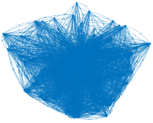
We test these algorithms over nodes connected via a directed network, which is a real Email network [46, 47]. Each node is associated with a local quadratic cost function where and are randomly sampled. Note that the quadratic cost function is commonly used in the literature [17, 24, 10]. The global constraint is .
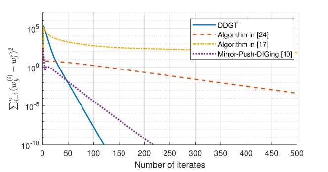
We first test the case without local constraints by setting . The stepsize used for each algorithm is tuned via a grid search222The grid search scheme works as follows. For each algorithm, we select a “good” stepsize by inspection, and then gradually increase and decrease stepsizes around the selected one with an equal grid size, respectively. Then, we find the fastest one among all the tried stepsizes. , and all initial conditions are randomly set. Fig. 2 depicts the decay of distance between and the optimal solution with respect to the number of iterations. It clearly shows that the DDGT has a linear convergence rate and converges faster than algorithms in [17, 24] and [10].
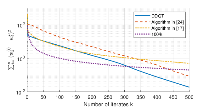
To validate the theoretical result for strongly convex cost functions without Lipschitz smoothness, we test the algorithms with a quartic local cost function , where and are randomly sampled. Clearly, this function is strongly convex but not Lipschitz smooth. All other settings remain the same and the result is plotted in Fig. 3, where the Mirror-Push-DIGing [10] is not included because its proximal operator is very time-consuming, and an approximate solution for the proximal operator often leads to a poor performance of the algorithm. The dotted line in Fig. 3 is the sequence with the number of iterations. We can observe that the convergence rates of all algorithms are slower than that in Fig. 2, but the DDGT still outperforms the other two algorithms. Moreover, it is interesting to observe that the DDGT and the algorithm in [24] have near-linear convergence rate, though the theoretical convergence rate for the DDGT is .
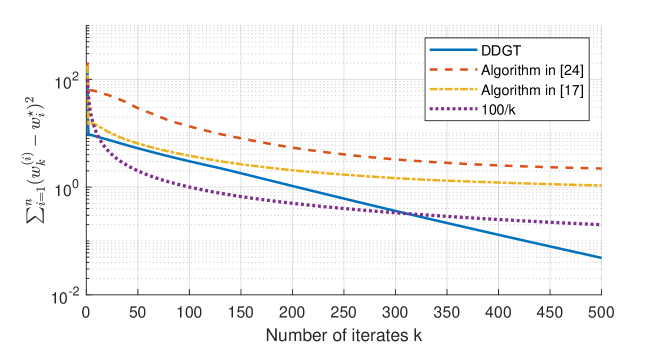
Finally, we study the effect of local constraints on the convergence rate. To this end, we assign each node a local constraint , and test all algorithms with the setting of Fig. 3. The result is depicted in Fig. 4, which shows that the convergence of the DDGT is essentially not affected, while the algorithm in [24] is heavily slowed compared with that in Fig. 3.
VI Conclusion
We proposed the DDGT for distributed resource allocation problems (DRAPs) over directed unbalanced networks. Convergence results are provided by exploiting the strong duality of DRAPs and distributed optimization problems, and taking advantage of the PPG algorithm. We studied the convergence and convergence rate of PPG for non-convex problems and obtained that the DDGT converges linearly for strongly convex and Lipschitz smooth objective functions, and sub-linearly without the Lipschitz smoothness. Future works are to provide tighter bounds for the convergence rate, design asynchronous versions [37, 38], study quantized communication [48], and design accelerated algorithms [49]. In particular, an interesting idea to accelerate the DDGT is to add a vanishing strongly convex regularization term to the dual problems of DRAPs, which may allow a larger stepsize in the early stage and hence possibly lead to faster convergence.
Acknowledgment
The authors would like to thank the Associate Editor and anonymous reviewers for their very constructive comments, which greatly improved the quality of this work.
-A Preliminary results on stochastic matrices
Lemma 1 ([26, 42])
Suppose Assumption 2 holds. The matrix has a unique unit nonnegative left eigenvector w.r.t. eigenvalue 1, i.e., and . The matrix has a unique unit right eigenvector w.r.t. eigenvalue 1, i.e., and .
Lemma 2 ([50],[25, 26])
Suppose Assumption 2 holds. There exist matrix norms and such that and . Moreover, and can be arbitrarily close to the second largest absolute value of the eigenvalues of and , respectively.
A method to construct such matrix norms can be found in the proof of Lemma 5.6.10 in [50].
Lemma 3 is a direct result of the norm equivalence theorem. If and are symmetric, which means the network is undirected, then and .
Note that the norm defined in Lemma 2 is only for matrices in . To facilitate presentation, we slightly abuse the notation and define a vector norm for any , where the norm in the right-hand-side is the matrix norm defined in Lemma 2. Then, we have
| (29) |
where the first equality is by definition and the inequality follows from the sub-multiplicativity of matrix norms. Moreover, for any matrix , define the matrix norm . Recall that is the dimension of and hence the definition is distinguished from that in Lemma 2. We have
| (30) | ||||
Therefore, for any , , and , the following relation holds
| (31) |
Similarly, we can obtain such a relation based on the matrix norm defined in Lemma 2.
Next, we define three important auxiliary variables:
| (32) |
where is a weighted average of that is identical to the one defined in Theorem 1, is a weighted average of , and is the sum of .
Finally, for any , let
| (33) |
and let denote the spectral radius of matrix .
-B Proof of Theorem 1
Step 1: Bound and
It follows from (11) that
| (34) | ||||
| (35) | ||||
| (36) | ||||
| (37) | ||||
| (38) | ||||
| (39) | ||||
| (40) | ||||
| (41) |
where we use Lemma 2 and (31) to obtain the first inequality, the second inequality is from Lemma 3 and (32), and the last inequality follows from the -Lipschitz smoothness.
Now we bound . From (15) we have
| (42) | ||||
where the last inequality follows from , which can be readily obtained from the construction of the norm [50, Lemma 5.6.10]. Moreover, it follows from (15a) that
| (43) | ||||
where we used . The above relation combined with (LABEL:eq2_s1) yields
| (44) | ||||
Combing (34) and (LABEL:eq1_s1) implies the following linear matrix inequality
| (45) | ||||
where denotes the element-wise less than or equal sign and
| (46) | ||||||
Note that for sufficiently small , since
| (47) |
has spectral radius smaller than 1.
The linear matrix inequality (LABEL:eq_lmi) implies that
| (48) |
Let and be the two eigenvalues of such that , and , then can be diagonalized as
| (49) |
Let Note that the analysis so far holds if is replaced by any value in (similar for ), and hence we assume without loss of generality that to simplify presentation. In that case, is lower bounded by some positive value that is independent of , say . With some tedious calculations, we have
| (50) | ||||
To let , it is sufficient for to satisfy
| (51) |
Moreover, and in (49) can be expressed in an explicit form
| (52) |
It then follows from (49) that
| (53) | ||||
where we used , and the bound (51) to obtain the inequality.
Combining (LABEL:eq_lmi), (48) and (LABEL:eq4_s1) yields that
| (54) | ||||
where and are constants given as follows
| (55) | ||||
Step 2: Bound
From (15) and the -Lipschitz smoothness, we have
| (56) |
Note that
| (57) | ||||
where we used the relation and . Then, we have
| (58) | ||||
where we used , and the Lipschitz smoothness to obtain the last inequality.
Moreover, it follows from (57) and the relation that
| (59) | ||||
Step 3: Bound and
Then, define
| (61) | ||||
| (62) | ||||
| (63) | ||||
| (64) |
where is defined in (50). Note that and , which combined with the relation and (LABEL:eq2_s3) yields
| (65) | ||||
The last term in (LABEL:eq7_s2) can be bounded by
| (66) |
where the last inequality follows from Thus, we have from (LABEL:eq7_s2) that
| (67) | ||||
Similarly, we can bound as follows,
| (68) | ||||
Next, we bound and . We first consider . For any , define
| (69) | ||||
where the elements are defined in (50) and (55). Clearly, is nonnegative and positive semi-definite. We have from (54) that , and hence
| (70) |
To bound , let be the element in the -th row and -th column of . For any , we have
| (71) | ||||
Since is symmetric, it holds that
| (72) | ||||
and we have from the Gershgorin circle theorem that
| (73) |
It then follows from (70) that
| (74) | ||||
Step 4: Bound
Summing both sides of (LABEL:eq3_s2) over , we have
| (76) | ||||
| (77) | ||||
where the last inequality follows from (LABEL:eq8_s2) and (LABEL:eq7_s4).
We can move the terms related to in the right-hand-side of (LABEL:eq2_s4) to the left-hand-side to bound . To this end, the stepsize should satisfy
| (78) | ||||
which is followed by
| (79) | ||||
If , i.e.,
| (80) |
then it follows from (LABEL:eq2_s4) that
| (81) | ||||
Thus, we have
| (82) | ||||
which is (LABEL:eq1_theo1) in Theorem 1. The inequality (17) follows from (LABEL:eq7_s4) immediately.
Now we look back at (LABEL:eq3_s2). Jointly with (LABEL:eq1_theo1), (LABEL:eq8_s2), (LABEL:eq7_s4) and (LABEL:eq3_s2), it follows from the supermartingale convergence theorem [41, Proposition A.4.4] that converges. If is further convex, it follows from the convergence of that converges to .
References
- [1] S. Yang, S. Tan, and J.-X. Xu, “Consensus based approach for economic dispatch problem in a smart grid,” IEEE Transactions on Power Systems, vol. 28, no. 4, pp. 4416–4426, 2013.
- [2] Y. Ho, L. Servi, and R. Suri, “A class of center-free resource allocation algorithms,” IFAC Proceedings Volumes, vol. 13, no. 6, pp. 475–482, 1980.
- [3] L. Xiao and S. Boyd, “Optimal scaling of a gradient method for distributed resource allocation,” Journal of optimization theory and applications, vol. 129, no. 3, pp. 469–488, 2006.
- [4] H. Lakshmanan and D. P. De Farias, “Decentralized resource allocation in dynamic networks of agents,” SIAM Journal on Optimization, vol. 19, no. 2, pp. 911–940, 2008.
- [5] C. Zhao, J. Chen, J. He, and P. Cheng, “Privacy-preserving consensus-based energy management in smart grids,” IEEE Transactions on Signal Processing, vol. 66, no. 23, pp. 6162–6176, 2018.
- [6] T. T. Doan and A. Olshevsky, “Distributed resource allocation on dynamic networks in quadratic time,” Systems & Control Letters, vol. 99, pp. 57–63, 2017.
- [7] T.-H. Chang, M. Hong, and X. Wang, “Multi-agent distributed optimization via inexact consensus ADMM,” IEEE Transactions on Signal Processing, vol. 63, no. 2, pp. 482–497, 2014.
- [8] T.-H. Chang, “A proximal dual consensus ADMM method for multi-agent constrained optimization,” IEEE Transactions on Signal Processing, vol. 64, no. 14, pp. 3719–3734, 2016.
- [9] N. S. Aybat and E. Y. Hamedani, “A Distributed ADMM-like Method for Resource Sharing over Time-Varying Networks,” SIAM Journal on Optimization, vol. 29, no. 4, pp. 3036–3068, 2019.
- [10] A. Nedić, A. Olshevsky, and W. Shi, “Improved convergence rates for distributed resource allocation,” in 2018 IEEE Conference on Decision and Control (CDC). IEEE, 2018, pp. 172–177.
- [11] J. Xu, S. Zhu, Y. C. Soh, and L. Xie, “A dual splitting approach for distributed resource allocation with regularization,” IEEE Transactions on Control of Network Systems, vol. 6, no. 1, pp. 403–414, 2018.
- [12] S. Liang, X. Zeng, G. Chen, and Y. Hong, “Distributed sub-optimal resource allocation via a projected form of singular perturbation,” arXiv preprint arXiv:1906.03628, 2019.
- [13] Y. Zhu, W. Ren, W. Yu, and G. Wen, “Distributed resource allocation over directed graphs via continuous-time algorithms,” IEEE Transactions on Systems, Man, and Cybernetics: Systems, 2019.
- [14] P. Xie, K. You, R. Tempo, S. Song, and C. Wu, “Distributed convex optimization with inequality constraints over time-varying unbalanced digraphs,” IEEE Transactions on Automatic Control, vol. 63, no. 12, pp. 4331–4337, 2018.
- [15] K. Cai and H. Ishii, “Average consensus on general strongly connected digraphs,” Automatica, vol. 48, no. 11, pp. 2750–2761, 2012.
- [16] Y. Xu, K. Cai, T. Han, and Z. Lin, “A fully distributed approach to resource allocation problem under directed and switching topologies,” in 2015 10th Asian Control Conference (ASCC). IEEE, 2015, pp. 1–6.
- [17] Y. Xu, T. Han, K. Cai, Z. Lin, G. Yan, and M. Fu, “A distributed algorithm for resource allocation over dynamic digraphs,” IEEE Transactions on Signal Processing, vol. 65, no. 10, pp. 2600–2612, 2017.
- [18] P. Li and J. Hu, “An ADMM based distributed finite-time algorithm for economic dispatch problems,” IEEE Access, vol. 6, pp. 30 969–30 976, 2018.
- [19] A. Falsone, I. Notarnicola, G. Notarstefano, and M. Prandini, “Tracking-ADMM for distributed constraint-coupled optimization,” arXiv preprint arXiv:1907.10860, 2019.
- [20] T. Yang, J. Lu, D. Wu, J. Wu, G. Shi, Z. Meng, and K. H. Johansson, “A distributed algorithm for economic dispatch over time-varying directed networks with delays,” IEEE Transactions on Industrial Electronics, vol. 64, no. 6, pp. 5095–5106, 2017.
- [21] X. Shi, Y. Wang, S. Song, and G. Yan, “Distributed optimisation for resource allocation with event-triggered communication over general directed topology,” International Journal of Systems Science, vol. 49, no. 6, pp. 1119–1130, 2018.
- [22] H. Zhang, H. Li, Y. Zhu, Z. Wang, and D. Xia, “A distributed stochastic gradient algorithm for economic dispatch over directed network with communication delays,” International Journal of Electrical Power & Energy Systems, vol. 110, pp. 759–771, 2019.
- [23] Y. Yuan, H. Li, J. Hu, and Z. Wang, “Stochastic gradient-push for economic dispatch on time-varying directed networks with delays,” International Journal of Electrical Power & Energy Systems, vol. 113, pp. 564–572, 2019.
- [24] H. Li, Q. Lü, and T. Huang, “Convergence analysis of a distributed optimization algorithm with a general unbalanced directed communication network,” IEEE Transactions on Network Science and Engineering, vol. 6, no. 3, pp. 237–248, 2019.
- [25] S. Pu, W. Shi, J. Xu, and A. Nedic, “Push-pull gradient methods for distributed optimization in networks,” IEEE Transactions on Automatic Control, pp. 1–1, 2020.
- [26] R. Xin and U. A. Khan, “A linear algorithm for optimization over directed graphs with geometric convergence,” IEEE Control Systems Letters, vol. 2, no. 3, pp. 315–320, July 2018.
- [27] F. Saadatniaki, R. Xin, and U. A. Khan, “Decentralized optimization over time-varying directed graphs with row and column-stochastic matrices,” IEEE Transactions on Automatic Control, pp. 1–1, 2020.
- [28] Y. Nesterov, Introductory lectures on convex optimization: A basic course. Springer Science & Business Media, 2013, vol. 87.
- [29] B. Gharesifard and J. Cortés, “When does a digraph admit a doubly stochastic adjacency matrix?” in American Control Conference, 2010. IEEE, 2010, pp. 2440–2445.
- [30] S. Boyd and L. Vandenberghe, Convex optimization. Cambridge university press, 2004.
- [31] D. Bertsekas, Nonlinear programming. Belmont, Massachusetts: Athena Scientific, 2016.
- [32] A. Nedić and A. Olshevsky, “Distributed optimization over time-varying directed graphs,” IEEE Transactions on Automatic Control, vol. 60, no. 3, pp. 601–615, 2015.
- [33] A. Nedić, A. Olshevsky, and W. Shi, “Achieving geometric convergence for distributed optimization over time-varying graphs,” SIAM Journal on Optimization, vol. 27, no. 4, pp. 2597–2633, 2017.
- [34] J. Zeng and W. Yin, “Extrapush for convex smooth decentralized optimization over directed networks,” Journal of Computational Mathematics, vol. 35, no. 4, pp. 383–396, 2017.
- [35] C. Xi and U. A. Khan, “DEXTRA: A fast algorithm for optimization over directed graphs,” IEEE Transactions on Automatic Control, vol. 62, no. 10, pp. 4980–4993, 2017.
- [36] V. S. Mai and E. H. Abed, “Distributed optimization over weighted directed graphs using row stochastic matrix,” in 2016 American Control Conference (ACC). IEEE, 2016, pp. 7165–7170.
- [37] J. Zhang and K. You, “AsySPA: An exact asynchronous algorithm for convex optimization over digraphs,” IEEE Transactions on Automatic Control, vol. 65, no. 6, pp. 2494–2509, 2020.
- [38] J. Zhang and K. You, “Asynchronous decentralized optimization in directed networks,” arXiv preprint arXiv:1901.08215, 2019.
- [39] X. Zhao and A. H. Sayed, “Asynchronous adaptation and learning over networks-Part I: Modeling and stability analysis,” IEEE Transactions on Signal Processing, vol. 63, no. 4, pp. 811–826, 2015.
- [40] T. Wu, K. Yuan, Q. Ling, W. Yin, and A. H. Sayed, “Decentralized consensus optimization with asynchrony and delays,” IEEE Transactions on Signal and Information Processing over Networks, vol. 4, no. 2, pp. 293–307, 2018.
- [41] D. P. Bertsekas, Convex Optimization Algorithms. Athena Scientific Belmont, 2015.
- [42] S. Pu and A. Nedić, “A distributed stochastic gradient tracking method,” in 2018 IEEE Conference on Decision and Control (CDC). IEEE, 2018, pp. 963–968.
- [43] Y. Zhao, X. He, and L. Chen, “A distributed strategy based on ADMM for dynamic economic dispatch problems considering environmental cost function with exponential term,” in IECON 2017-43rd Annual Conference of the IEEE Industrial Electronics Society. IEEE, 2017, pp. 7387–7392.
- [44] L. Zheng and C. W. Tan, “Optimal algorithms in wireless utility maximization: Proportional fairness decomposition and nonlinear perron-frobenius theory framework,” IEEE Transactions on Wireless Communications, vol. 13, no. 4, pp. 2086–2095, 2014.
- [45] J.-B. Hiriart-Urruty and C. Lemaréchal, Conjugacy in Convex Analysis. Berlin, Heidelberg: Springer Berlin Heidelberg, 1993, pp. 35–90. [Online]. Available: https://doi.org/10.1007/978-3-662-06409-2_2
- [46] “Manufacturing emails network dataset – KONECT,” Sep. 2016. [Online]. Available: http://konect.uni-koblenz.de/networks/radoslaw_email
- [47] J. Kunegis, “KONECT – The Koblenz Network Collection,” in Proc. Int. Conf. on World Wide Web Companion, 2013, pp. 1343–1350. [Online]. Available: http://userpages.uni-koblenz.de/~kunegis/paper/kunegis-koblenz-network-collection.pdf
- [48] J. Zhang, K. You, and T. Başar, “Distributed discrete-time optimization in multiagent networks using only sign of relative state,” IEEE Transactions on Automatic Control, vol. 64, no. 6, pp. 2352–2367, 2018.
- [49] G. Qu and N. Li, “Accelerated distributed Nesterov gradient descent,” IEEE Transactions on Automatic Control, pp. 1–1, 2019.
- [50] R. A. Horn and C. R. Johnson, Matrix analysis. Cambridge university press, 2012.
![[Uncaptioned image]](/html/1909.09937/assets/x5.png) |
Jiaqi Zhang received the B.S. degree in electronic and information engineering from the School of Electronic and Information Engineering, Beijing Jiaotong University, Beijing, China, in 2016. He is currently pursuing the Ph.D. degree at the Department of Automation, Tsinghua University, Beijing, China. His research interests include networked control systems, distributed or decentralized optimization and their applications. |
![[Uncaptioned image]](/html/1909.09937/assets/x6.png) |
Keyou You (SM’17) received the B.S. degree in Statistical Science from Sun Yat-sen University, Guangzhou, China, in 2007 and the Ph.D. degree in Electrical and Electronic Engineering from Nanyang Technological University (NTU), Singapore, in 2012. After briefly working as a Research Fellow at NTU, he joined Tsinghua University in Beijing, China where he is now a tenured Associate Professor in the Department of Automation. He held visiting positions at Politecnico di Torino, Hong Kong University of Science and Technology, University of Melbourne and etc. His current research interests include networked control systems, distributed optimization and learning, and their applications. Dr. You received the Guan Zhaozhi award at the 29th Chinese Control Conference in 2010 and the ACA (Asian Control Association) Temasek Young Educator Award in 2019. He was selected to the National 1000-Youth Talent Program of China in 2014 and received the National Science Fund for Excellent Young Scholars in 2017. He is serving as an Associate Editor for the IEEE Transactions on Cybernetics, IEEE Control Systems Letters(L-CSS), Systems & Control Letters. |
![[Uncaptioned image]](/html/1909.09937/assets/x7.png) |
Kai Cai (S’08-M’12-SM’17) received the B.Eng. degree in Electrical Engineering from Zhejiang University, Hangzhou, China, in 2006; the M.A.Sc. degree in Electrical and Computer Engineering from the University of Toronto, Toronto, ON, Canada, in 2008; and the Ph.D. degree in Systems Science from the Tokyo Institute of Technology, Tokyo, Japan, in 2011. He is currently an Associate Professor at Osaka City University. Previously, he was an Assistant Professor at the University of Tokyo (2013-2014), and a postdoctoral Fellow at the University of Toronto (2011-2013). Dr. Cai’s research interests include distributed control of discrete-event systems and cooperative control of networked multi-agent systems. He is the co-author (with W.M. Wonham) of Supervisory Control of Discrete-Event Systems (Springer 2019) and Supervisor Localization (Springer 2016). He is serving as an Associate Editor for the IEEE Transactions on Automatic Control. |