Structured Binary Neural Networks for Image Recognition

Abstract

In this paper, we propose to train binarized convolutional neural networks (CNNs) that are of significant importance for deploying deep learning to mobile devices with limited power capacity and computing resources. Previous works on quantizing CNNs often seek to approximate the floating-point information of weights and/or activations using a set of discrete values. Such methods, termed value approximation here, typically are built on the same network architecture of the full-precision counterpart. Instead, we take a new “structured approximation” view for network quantization — it is possible and valuable to exploit flexible architecture transformation when learning low-bit networks, which can achieve even better performance than the original networks in some cases. In particular, we propose a “group decomposition” strategy, termed GroupNet, which divides a network into desired groups. Interestingly, with our GroupNet strategy, each full-precision group can be effectively reconstructed by aggregating a set of homogeneous binary branches. We also propose to learn effective connections among groups to improve the representation capability. To improve the model capacity, we propose to dynamically execute sparse binary branches conditioned on input features while preserving the computational cost. More importantly, the proposed GroupNet shows strong flexibility for a few vision tasks. For instance, we extend the GroupNet for accurate semantic segmentation by embedding the rich context into the binary structure. The proposed GroupNet also shows strong performance on object detection. Experiments on image classification, semantic segmentation, and object detection tasks demonstrate the superior performance of the proposed methods over various quantized networks in the literature. Moreover, the speedup and runtime memory cost evaluation comparing with related quantization strategies is analyzed on GPU platforms, which serves as a strong benchmark for further research.

1 Introduction

Deep convolutional neural networks have achieved significant breakthroughs in many machine learning tasks, such as image classification he2016deep , object segmentation long2015fully ; chen2018encoder and object detection tian2019fcos . However, deep models often require billions of FLOPs for inference, which makes them infeasible for many real-time applications especially on resource constrained mobile platforms. To solve this, existing works focus on network pruning zhuang2018discrimination ; he2017channel ; lin2019towards , low-bit quantization zhuang2018towards ; jacob2017quantization and/or efficient architecture design chollet2017xception ; howard2017mobilenets . Among them, quantization approaches seek to represent the weights and/or activations with low bitwidth fixed-point integers. Thus, the dot product can be computed by several XNOR-popcount bitwise operations. Binarization hubara2016binarized ; rastegari2016xnor , which is an extreme quantization approach, seeks to represent the weights and activations by a single bit (e.g., $+1$ or $-1$). Binarization has gained great attention recently since the XNOR of two bits can be executed extremely fast ehliar2014area ; govindu2004analysis . In this paper, we aim to design highly accurate binary neural networks (BNNs) from a new quantization perspective.

Existing fixed-point quantization methods, including binarization, seek to quantize weights and/or activations by preserving most of the representational ability of the original network. In this sense, these methods are based on the idea of value approximation, which can be mainly divided into two categories. The first category design effective optimization algorithms to find better local minima for quantized weights. These works either introduce knowledge distillation zhuang2018towards ; polino2018model ; mishra2018apprentice or use loss-aware objectives hou2018loss ; hou2017loss . The second category approaches focus on improving the quantizer zhou2016dorefa ; Cai_2017_CVPR ; zhang2018lq , by learning suitable mappings between discrete values and their floating-point counterparts.

Note that, these value approximation based approaches may have a natural limitation as it is merely a sub-optimal approximation to the original network. Moreover, designing a good quantization function is highly non-trivial especially for BNNs, since the quantization process essentially is non-differentiable and the gradients can only be roughly approximated. Last, these methods often lack of adaptive ability for other vision tasks beyond image classification. Often these methods may work well on image classification tasks, but may not achieve promising quantization performance on segmentation and detection tasks.

In this paper, we investigate the task of quantization from a new perspective of structured approximation. We observe that, instead of directly approximating the original network, it is possible, and valuable to learn an ensemble of a set of binary bases that can match the representational capability of the floating-point model. In particular, we propose a “group decomposition” strategy termed GroupNet, which partitions a full-precision model into groups. For the sake of exposition, we use terminology for network architectures as comprising layers, blocks and groups. A layer is a standard single parameterized layer in a network such as a dense or convolutional layer, except with binary weights and activations. A block is a collection of layers in which the output of end layer is connected to the input of the next block (e.g., a residual block). A group is a collection of blocks. In particular, one of the key points is, based on the proposed GroupNet strategy, we are able to use a set of binary bases to well approximate the floating-point model. This design shows three benefits.

First, GroupNet enables more flexible trade-off between computational complexity and accuracy. Specifically, GroupNet enables fine-grained quantization levels that can be any positive integers (except 1) while fixed-point methods zhuang2018towards ; zhou2016dorefa require the quantization levels to be exponential power of 2. As a result, GroupNet can achieve the fine-grained bit-width by directly controlling the number of bases, which works better for balancing the efficiency and accuracy of the overall network.

Second, skip connections have been shown to be important in increasing representational power and improving gradient backpropagation as demonstrated in BNNs literature Liu_2018_ECCV . In this sense, our group-wise design enjoys $K$ times more skip connections than value approximation, where $K$ is the number of bases.

Third, the higher-level structural information can be better utilized than the value approximation approaches. In practice, while the value approximation based approaches show promising performance on image classification tasks, they often perform poorly on more challenging tasks such as semantic segmentation and object detection. Relying on the proposed group decomposition strategy, we are able to exploit task-specific information or structures and further design flexible binary structures according to specific tasks to compensate the quantization loss for general tasks.

Specifically, for semantic segmentation, we are motivated by Atrous Spatial Pyramid Pooling (ASPP) chen2017rethinking ; chen2018encoder , which is built on top of extracted features of the backbone network. To capture the multi-scale context, we propose to directly apply different atrous rates on parallel binary bases in the backbone network, which is equivalent to absorbing ASPP into the feature extraction stage. As will be shown, our strategy significantly boosts the performance on semantic segmentation without increasing much computational complexity of the binary convolutions. Moreover, we further extend the proposed approach to building quantized networks for object detection. Building low-precision networks for object detection is more challenging since detection needs the network to output richer information, locations and categories of bounding boxes. Several works in literature address quantized object detection jacob2017quantization ; li2019fully ; wei2018quantization . There is still a considerable performance gap between quantized object detectors and their full-precision counterparts. To tackle this problem, we apply our GroupNet and propose a new design modification to better accommodate the quantized object detector and achieve improved detection accuracy. Last, it is worth mentioning that our structured approximation strategy and the value approximation strategy are complementary rather than contradictory. In fact, both are important and should be exploited to obtain highly accurate BNNs.

In this paper, we propose to redesign binary network architectures from the quantization view. We highlight that while most existing quantization works focus on directly quantizing the full-precision architecture, we begin to explore alternative architectures that shall be better suited for dealing with binary weights and activations. In particular, apart from decomposing each group into several binary bases, we also propose to learn the connections between each group by introducing a soft fusion gate. To further increase model capacity while preserving the computational cost, we propose to tailor conditional computing to binary networks by learning to select informative bases for each group conditioned on input features.

Our main contributions are summarized as follows.

• We propose to design accurate BNNs structures from the structured approximation perspective. Specifically, we divide the network into groups and approximate each group using a set of binary bases. We also propose to automatically learn the decomposition by introducing soft connections.

• We explore ideas from conditional computing to learn adaptive, conditional binary bases, which are dynamically selected during inference conditioned on the input features. This strategy significantly increases the model capacity of GroupNet without increasing computational complexity during inference.

• The proposed GroupNet has strong flexibility and can be easily extended to tasks other than image classification. For instance, we propose Binary Parallel Atrous Convolution (BPAC), which embeds rich multi-scale context into BNNs for semantic segmentation. GroupNet with BPAC significantly improves the performance while maintaining the complexity compared to employ GroupNet only.

• To our knowledge, we are among the pioneering approaches to apply binary neural networks to general semantic segmentation and object detection tasks.

• We develop implementations to evaluate the execution speed and runtime memory cost of GroupNet and make comparison with other bit configurations on various platforms.

• We evaluate our models on ImageNet, PASCAL VOC and COCO datasets based on various architectures. Experiments show that the proposed GroupNet achieves the state-of-the-art trade-off between accuracy and computational complexity.

This paper extends our preliminary results in zhuang2019structured in several aspects. 1) In the conference version, we propose to employ the soft routing mechanism to learn group-wise connections. Nevertheless, all the branches still need to be executed at test time. In this paper, we further explore more advanced structured approximation for BNNs. As opposed to static ones, we adapt the structures to the input during inference, with enlarged parameter space and improved model capacity. In particular, we employ conditional computation by optimizing data-dependent binary gates to decide the execution of branches in each group. 2) We develop the acceleration code on resource constrained platforms and evaluate speedup and runtime memory cost comparing with various quantization methods. 3) We make more analysis on differences and advantages of GroupNet over other related quantization strategies. 4) In addition to image classification and semantic segmentation, we further extend GroupNet to object detection. In particular, we propose several modifications to quantized object detection and our GroupNet outperforms the comparison methods. 5) For image classification, we conduct more ablation studies and experiments on more architectures and provide detailed analysis. 6) For semantic segmentation, we develop models based on DeepLabv3 and provide useful instructions.

2 Related Work

Network quantization. The recent increasing demand for implementing fixed-point deep neural networks on embedded devices motivates the study of low-bit network quantization. Quantization based methods represent the network weights and/or activations with very low precision, thus yielding highly compact DNN models compared to their floating-point counterparts. BNNs hubara2016binarized ; rastegari2016xnor propose to constrain both weights and activations to binary values (i.e., $+1$ and $-1$), where the multiplication-accumulations can be replaced by purely $\rm xnor(\cdot)$ and $\rm popcount(\cdot)$ operations, which are in general much faster. However, BNNs still suffer from significant accuracy decrease compared with the full precision counterparts. To narrow this accuracy gap, ternary networks li2016ternary ; zhu2016trained and even higher bit fixed-point quantization zhou2016dorefa ; zhou2017incremental methods are proposed.

In general, quantization approaches target at tackling two main problems. On one hand, some works target at designing a more accurate quantizer to minimize information loss. For the uniform quantizer, works in choi2018pact ; jung2019learning explicitly parameterize and optimize the upper and/or lower bound of the activation and weights. To reduce the quantization error, non-uniform approaches park2017weighted ; zhang2018lq are proposed to better approximate the data distribution. In particular, LQ-Net zhang2018lq proposes to jointly optimize the quantizer and the network parameters. On the other hand, because of the non-differentiable quantizer, some literature focuses on relaxing the discrete optimization problem. A typical approach is to train with regularization ding2019regularizing ; bai2019proxquant , where the optimization problem becomes continuous while gradually adjusting the data distribution towards quantization level. Moreover, Hou et al.  hou2017loss ; hou2018loss propose the loss-aware quantization by directly optimizing the discrete objective function.

To well balance accuracy and complexity, several works guo2017network ; li2017performance ; lin2017towards ; fromm2018heterogeneous ; tang2017train propose to employ a linear combination of binary tensors to approximate the filters and/or activations while still possessing the advantage of binary operations. In particular, Guo et al.  guo2017network recursively perform residual quantization on pretrained full-precision weights and do convolution on each binary weight base. Similarly, Li et al.  li2017performance propose to expand the input feature maps into binary bases in the same manner. Lin et al.  lin2017towards further expand both weights and activations with a simple linear approach. Unlike the previous local tensor approximation approaches, we propose to design BNNs from a structured approximation perspective and show strong generalization on a few mainstream computer vision tasks.

There also have been several works that employ neural architecture search (NAS) for BNNs bulat2020bats ; zhu2020nasb ; chen2020binarized ; ding2020bnas to explore a high-performance binary neural architecture. Note that our GroupNet is orthogonal to these approaches, where we explore how to ensemble the binary bases effectively to approximate the original full-precision network. Based on an advanced binary base architecture, our GroupNet can achieve better performance.

Hardware Implementation. In addition to the quantization algorithms design, the implementation frameworks and acceleration libraries ignatov2018ai ; chen2018tvm ; umuroglu2017finn ; jacob2017quantization ; yang2017bmxnet are indispensable to expedite the quantization technique to be deployed on energy-efficient edge devices. For example, TBN Wan_2018_ECCV focuses on the implementation of ternary activation and binary weight networks. daBNN zhang2019dabnn targets at the inference optimization of BNNs on ARM CPU devices. GXNOR-Net deng2018gxnor treats TNNs as sparse BNNs and propose an acceleration solution on dedicated hardware platforms. In this paper, we develop the acceleration code for BNNs, GroupNet and fixed-point quantization on GPU platforms. We also compare the accuracy and efficiency trade-offs between them.

Dynamic networks. Dynamic networks, as opposed to static ones, can adapt their structures or parameters to the input during inference, and therefore enjoy desired trade-off between accuracy and efficiency for dealing with varying computational budgets on the fly. In particular, closely related to our paper, mixture of experts (MoE) jacobs1991adaptive ; jordan1994hierarchical build multiple network branches as experts in parallel. For example, HydraNet mullapudi2018hydranets replaces the convolutional blocks in the last stage of a CNN by multiple branches, and selectively execute these branches at test time. The recent Switch Transformer fedus2021switch proposes to dynamically activate a FFN layer from experts, leading to trillion parameter models with constant computational cost. In this paper, we tailor conditional computing to GroupNet by learning to select data-specific bases for each group. Related to our GroupNet, High-capacity Expert BNNs (HCE) bulat2021high proposes to automatically search for optimal binary network architectures, equipped with multiple experts to increase model capacity. During inference, HCE only selects one expert, while our GroupNet enables Top-$N$ selection for larger model capacity. Moreover, our GroupNet focuses on structured experts, while the scope of HCE is on designing layer-wise experts for binary convolutions.

Semantic segmentation. Deep learning based semantic segmentation is popularized by the Fully Convolutional Networks (FCNs) long2015fully . Recent prominent directions have emerged: using the encoder-encoder structure zhang2018exfuse ; chen2018encoder ; relying on dilated convolutions to keep the reception fields without downsampling the spatial resolution too much chen2017rethinking ; mehta2018espnet ; employing multi-scale feature fusion lin2017refinenet ; chen2018deeplab ; employment of probabilistic graphical models lin2016efficient ; chandra2016fast .

However, these approaches typically focus on designing complex modules for improving accuracy while sacrificing the inference efficiency to some extent. To make semantic segmentation applicable, several methods have been proposed to design real-time semantic segmentation models. Recently, works of liu2019auto ; nekrasov2019fast apply neural architecture search for exploring more accurate models with less Multi-Adds operations. Yu et al.  yu2018bisenet propose BiSeNet, where a spatial path extracts high resolution features and a context path obtains sufficient receptive fields to achieve high speed and accuracy. ESPNet mehta2018espnet ; mehta2018espnetv2 design efficient spatial pyramid for real-time semantic segmentation under resource constraints. In contrast, we instead propose to accelerate semantic segmentation frameworks from the quantization perspective, which is parallel to the above approaches. Given a pretrained full-precision model, we can replace multiplication-accumulations by the XNOR-popcount operations, which would bring great benefits for embedded platforms. We may be the first to apply binary neural networks on semantic segmentation and achieve promising results.

Object detection. Object detection has shown great success with deep neural networks. As one of the dominant detection framework, two-stage detection methods girshick2015fast ; girshick2014rich ; ren2015faster first generate region proposals and then refine them by subsequent networks. The popular method Faster-RCNN ren2015faster first proposes an end-to-end detection framework by introducing a region proposal network (RPN). Another main category is the one-stage methods which are represented by YOLO redmon2016you ; redmon2017yolo9000 ; redmon2018yolov3 , SSD liu2016ssd and FCOS tian2019fcos . The objective is to improve the detection efficiency by directly classifying and regressing the pre-defined anchors without the proposal generation step. RetinaNet lin2017focal proposes a new focal loss to tackle the extreme foreground-background class imbalance encountered during training in one-stage detectors. Moreover, Tian et al.  tian2019fcos propose a simple fully convolutional anchor-free one-stage detector that achieves on par performance with the anchor-based one-stage detectors.

In addition, designing light-weight detection frameworks is crucial since mobile applications usually require real-time, low-power and fully embeddable. For example, the work of chen2017learning and wei2018quantization propose to train a tiny model by distilling knowledge from a deeper teacher network. MNasNet tan2018mnasnet proposes to automatically search for mobile CNNs which achieve improved mAP quality than MobileNets for object detection. In this paper, we explore to design efficient detectors from the quantization view. Note that, we are probably the first to train a binary object detection model.

3 Proposed Method

Most previous methods in the literature have focused on value approximation by designing accurate binarization functions for weights and activations (e.g., multiple binarizations lin2017towards ; tang2017train ; guo2017network ; li2017performance ; fromm2018heterogeneous ). In this paper, we seek to binarize both weights and activations of CNNs from a “group-wise approximation” view. In the following, we first define the research problem and present some basic knowledge about binarization in Section 3.1. Then, we explain our binary architecture design strategy in Section 3.2 and introduce how to learn architectures automatically and dynamically in Section 3.3. In Section 3.4, we further provide the complexity analysis. Finally, in Section 3.5 and Section 3.6, we describe how to use task-specific attributes to generalize our approach to semantic segmentation and object detection, respectively.

3.1 Problem definition

For a convolutional layer, we define the input feature ${\bf{x}}\in{\mathbb{R}^{{c_{in}}\times{w_{in}}\times{h_{in}}}}$, weight tensor ${\bf{w}}\in{\mathbb{R}^{{c_{in}}\times{c_{out}}\times w\times h}}$ and the output ${\bf{y}}\in{\mathbb{R}^{{c_{out}}\times{w_{out}}\times{h_{out}}}}$, respectively.

Binarization of weights: Following  rastegari2016xnor , we approximate the floating-point weight ${\bf{w}}$ by a binary weight filter ${{\bf{b}}^{w}}$ and a scaling factor $\alpha\in{\mathbb{R}^{+}}$ such that ${\bf{w}}\approx\alpha{{\bf{b}}^{w}}$, where ${{\bf{b}}^{w}}$ is the sign of ${\bf{w}}$ and $\alpha$ calculates the mean of absolute values of ${\bf{w}}$. In general, $\rm sign(\cdot)$ is non-differentiable and so we adopt the straight-through estimator bengio2013estimating (STE) to approximate the gradient calculation. Formally, the forward and backward processes can be written as follows:

$$\begin{split}&\mbox{Forward}:{{\bf{b}}^{w}}={\rm{sign}}({\bf{w}}),\\ &\mbox{Backward}:\frac{{\partial\ell}}{{\partial{\bf{w}}}}=\frac{{\partial\ell}}{{\partial{{\bf{b}}^{w}}}}\cdot\frac{{\partial{{\bf{b}}^{w}}}}{{\partial{\bf{w}}}}\approx\frac{{\partial\ell}}{{\partial{{\bf{b}}^{w}}}},\\ \end{split}$$ (1)

where $\ell$ is the loss.

Binarization of activations: For activation binarization, we utilize the piecewise polynomial function to approximate the sign function as in Liu_2018_ECCV . The forward and backward can be written as:

$$\begin{array}[]{l}\mbox{Forward}:{b^{a}}={\rm{sign}}(x),\\ \mbox{Backward}:\frac{{\partial\ell}}{{\partial x}}=\frac{{\partial\ell}}{{\partial{b^{a}}}}\cdot\frac{{\partial{b^{a}}}}{{\partial x}},\\ \mbox{where}\quad\frac{{\partial{b^{a}}}}{{\partial x}}=\left\{\begin{array}[]{l}2+2x:-1\leq x<0\\ 2-2x:0\leq x<1\\ 0:\rm{otherwise}\end{array}\right..\end{array}$$ (2)

3.2 Binary Network Decomposition

In this paper, we want to design a new structural representation of a network for quantization. First of all, note that a float number in computer is represented by a fixed-number of binary digits. Motivated by this, rather than directly doing the quantization via “value decomposition”, we propose to decompose a network into binary structures while preserving its representability.

Specifically, given a floating-point residual network $\Phi(\cdot)$ with $N$ blocks, we decompose $\Phi(\cdot)$ into $P$ binary fragments $[{{\cal F}_{1}},...,{{\cal F}_{P}}]$, where ${{\cal F}_{i}}(\cdot)$ can be any binary structure. Note that each ${{\cal F}_{i}}(\cdot)$ can be different. A natural question arises: can we find some simple methods to decompose the network with binary structures so that the representability can be exactly preserved? To answer this question, we here explore two kinds of architectures for ${{\cal F}}(\cdot)$, namely layer-wise decomposition and group-wise decomposition in Section 3.2.1 and Section 3.2.2, respectively. Then we present a novel strategy for automatic decomposition in Section 3.3.

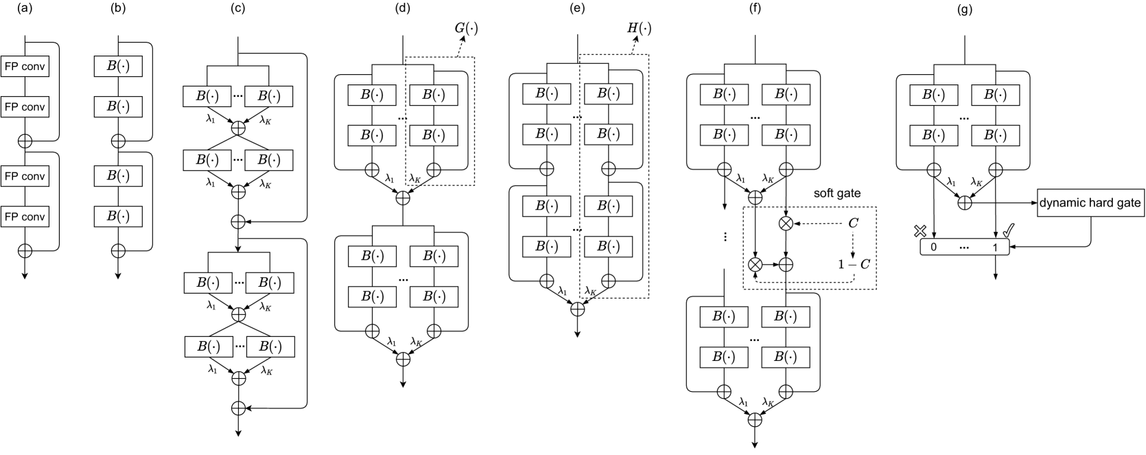
Figure 1: Illustration of the proposed method. We take one residual block with two convolutional layers for illustration. For convenience, we omit batch normalization and nonlinearities. (a): The floating-point residual block. (b): Direct binarization of a full-precision block. (c): Layer-wise binary decomposition in Eq. (3), where we use a set of binary convolutional layers $B(\cdot)$ to approximate a floating-point convolutional layer. (d): Basic group-wise binary decomposition in Eq. (5), where we approximate a whole block with a linear combination of binary blocks $G(\cdot)$. (e): We approximate a whole group with homogeneous binary bases $H(\cdot)$, where each group consists of several blocks. This corresponds to Eq. (6). (f): Illustration of the soft connection between two neighbouring blocks. (g): Hard gating mechanism for dynamically selecting branches.

3.2.1 Layer-wise binary decomposition

The key challenge of binary decomposition is how to reconstruct or approximate the floating-point structure. The simplest way is to approximate in a layer-wise manner. Let $B(\cdot)$ be a binary convolutional layer and ${\bf{b}}_{i}^{w}$ be the binarized weights for the $i$-th base. In Figure 1(c), we illustrate the layer-wise feature reconstruction for a single block. Specifically, for each layer, we aim to fit the full-precision structure using a set of binarized homogeneous branches ${\cal F(\cdot)}$ given a floating-point input tensor $\bf{x}$:

$${{\cal F}}({\bf{x}})=\frac{1}{K}\sum\limits_{i=1}^{K}{B_{i}}({\bf{x}})=\frac{1}{K}\sum\limits_{i=1}^{K}({\bf{b}}_{i}^{w}\oplus{\rm{sign}}({\bf{x}})),$$ (3)

where $\oplus$ is bitwise operations $\rm xnor(\cdot)$ and $\rm popcount(\cdot)$, $K$ is the number of branches. During the training, the structure is fixed and each binary convolutional kernel ${\bf{b}}_{i}^{w}$ is directly updated with end-to-end optimization. The scale scalar can be absorbed into batch normalization when doing inference. Note that all ${{B_{i}}}$’s in Eq. (3) have the same topology as the original floating-point counterpart. Each binary branch gives a rough approximation and all the approximations are aggregated to achieve more accurate reconstruction to the original full precision convolutional layer. Note that when $K=1$, it corresponds to directly binarize the floating-point convolutional layer (Figure 1 (b)). However, with more branches (a larger $K$), we are expected to achieve more accurate approximation with more complex transformations.

Different from zhuang2019structured , we remove the floating-point scales for two reasons. First, the scales can be absorbed into batch normalization layers. Second, we empirically observe that the learnt scales for different branches differ a little and removing them does not influence the performance.

During the inference, the homogeneous $K$ bases can be parallelizable and thus the structure is hardware friendly. This will bring significant gain in speed-up of the inference. Specifically, the bitwise XNOR operation and bit-counting can be performed in a parallel of 64 by the current generation of CPUs rastegari2016xnor ; Liu_2018_ECCV . We only need to calculate $K$ binary convolutions and $K$ full-precision additions. As a result, the speed-up ratio $\sigma$ for a convolutional layer can be calculated as:

$$\sigma=\frac{{64{c_{{in}}}\cdot w\cdot h\cdot{w_{in}}\cdot{h_{in}}}}{K({{c_{{in}}}\cdot w\cdot h\cdot{w_{in}}\cdot{h_{in}}+64{w_{out}}\cdot{h_{out}}})}.$$ (4)

We take one layer in ResNet for example. If we set ${c_{in}}=256$, $w\times h=3\times 3$, ${w_{in}}={h_{in}}={w_{out}}={h_{out}}=28$, $K=5$, then it can reach 12.45$\times$ speedup. In practice, the actual speedup ratio is also influenced by the process of memory read and thread communication. We extensively evaluate the on-device speedup in Section 6.

3.2.2 Group-wise binary decomposition

In the layer-wise approach, we approximate each layer with multiple branches of binary layers. Note each branch will introduce a certain amount of error and the error may accumulate due to the aggregation of multi-branches. As a result, this strategy may incur severe quantization errors and bring large deviation for gradients during back-propagation. To alleviate the above issue, we further propose a more flexible decomposition strategy called group-wise binary decomposition, to preserve more structural information during approximation.

To explore the group-structure decomposition, we first consider a simple case where each group consists of only one block. Then, the layer-wise approximation strategy can be easily extended to the group-wise case. As shown in Figure 1 (d), similar to the layer-wise case, each floating-point group is decomposed into multiple binary groups. However, each group ${G_{i}(\cdot)}$ is a binary block which consists of several binary convolutions and fixed-point operations (i.e., AddTensor). For example, we can set ${G_{i}(\cdot)}$ as the basic residual block he2016deep which is shown in Figure 1 (a). Considering the residual architecture, we can decompose ${\cal F}({\bf{x}})$ by extending Eq. (3) as:

$${\cal F}({\bf{x}})=\frac{1}{K}\sum\limits_{i=1}^{K}{G_{i}}({\bf{x}}).$$ (5)

In Eq. (5), we use a linear combination of homogeneous binary bases to approximate one group, where each base ${G_{i}}$ is a binarized block. Thus, we effectively keep the original residual structure in each base to preserve the network capacity. As shown in Section 5.2.2, the group-wise decomposition strategy performs much better than the simple layer-wise approximation.

Furthermore, the group-wise approximation is flexible. We now analyze the case where each group may contain different number of blocks. Suppose we partition the network into $P$ groups and it follows a simple rule that each group must include one or multiple complete residual building blocks. For the $p$-th group, we consider the blocks set $T\in\{{T_{p-1}}+1,...,{T_{p}}\}$, where the index ${T_{p-1}}=0$ if $p=1$. We can extend Eq. (5) into multiple blocks format:

$$\begin{array}[]{l}{\cal F}({{\bf{x}}_{{T_{p-1}}+1}})=\frac{1}{K}\sum\limits_{i=1}^{K}{H_{i}}({\bf{x}}),\\ =\frac{1}{K}\sum\limits_{i=1}^{K}{G_{i}^{{T_{p}}}(G_{i}^{{T_{p}}-1}(...(G_{i}^{{T_{p-1}}+1}({{\bf{x}}_{{T_{p-1}}+1}}))...)}),\end{array}$$ (6)

where $H(\cdot)$ is a cascade of consequent blocks which is shown in Figure 1 (e). Based on ${\cal{F(\cdot)}}$, we can efficiently construct a network by stacking these groups and each group may consist of one or multiple blocks. Different from Eq. (5), we further expose a new dimension on each base, which is the number of blocks. This greatly increases the structure space and the flexibility of decomposition. We explore the effect of the structure space in Section 5.2.2 and further describe how to learn the decomposition in Section 3.3.

3.3 Learning for decomposition

There is a significant challenge involved in Eq. (6). Note that the network has $N$ blocks and the possible number of connections is ${2^{N}}$. Clearly, it is not practical to enumerate all possible structures during the training. Here, we propose to solve this problem by learning the structures for decomposition automatically.

3.3.1 Learned soft gating

We introduce in a fusion gate as the soft connection between blocks $G(\cdot)$. To this end, we first define the input of the $i$-th branch for the $n$-th block as:

$$C_{i}^{n} =\mathrm{sigmoid}({\theta^{n}_{i}}),$$ (7)

$${\bf{x}}_{i}^{n} ={C^{n}_{i}}\odot G_{i}^{n-1}({\bf{x}}_{i}^{n-1})$$

$$+(1-{C^{n}_{i}})\odot\sum\limits_{j=1}^{K}G_{j}^{n-1}({\bf{x}}_{j}^{n-1}),$$

where $\mbox{{\boldmath$\theta$}}\in{\mathbb{R}^{K}}$ is a learnable parameter vector, $C_{i}^{n}$ is a gate scalar and $\odot$ is the Hadamard product. And we empirically observe that using a learnable scale $\theta$ that shares among branches does not influence the performance and it can be absorbed into batch normalization (BN) layers during inference.

Here, the branch input ${\bf{x}}_{i}^{n}$ is a weighted combination of two paths. The first path is the output of the corresponding $i$-th branch in the $(n-1)$-th block, which is a direct connection. The second path is the aggregation output of the $(n-1)$-th block. The detailed structure is shown in Figure 1 (f). In this way, we make more information flow into the branch and increase the gradient paths for improving the convergence of BNNs.

Remarks: For the extreme case when $\sum\nolimits_{i=1}^{K}{C_{i}^{n}}=0$, Eq. (7) will be reduced to Eq. (5) which means we approximate the $(n-1)$-th and the $n$-th block independently. When $\sum\nolimits_{i=1}^{K}{{C_{i}^{n}}}=K$, Eq. (7) is equivalent to Eq. (6) and we set $H(\cdot)$ to be two consequent blocks and approximate the group as a whole. Interestingly, when $\sum\nolimits_{n=1}^{N}{\sum\nolimits_{i=1}^{K}{C_{i}^{n}}}=NK$, it corresponds to set $H(\cdot)$ in Eq. (6) to be a whole network and directly ensemble $K$ binary models.

Note that the group-wise decomposition has $K\times$ more skip connections than the layer-wise decomposition, implying the improved representational power and gradient backpropagation of the model.

3.3.2 Dynamic hard gating

The soft gating regime in Section 3.3.1 adopts real-valued weights to dynamically rescale the representations obtained from different branches. In this way, all the branches still need to be executed, and the computation cannot be reduced at test time. To improve the inference efficiency, we propose to learn dynamic hard gates, allowing the models to adaptively allocate the computation dependent on the input features with only a fraction of activated branches. Such a design is shown in Figure 1 (g). Formally, the gating mechanism is applied to the output of the preceding group and can be formulated as

$$g_{i}=\begin{cases}1,&\text{ if }\psi({\bf x})_{i}\geq f(\psi({\bf x}),N)\\ 0,&\text{ otherwise }\end{cases}$$ (8)

where $g_{i}$ is the $i$-th element of a $K$-dimensional binary vector ${\bf g}$ which is used to select the $N$ activated branches, $\psi(\cdot)$ is a learned mapping function of the input ${\bf x}$ and $f(\psi({\bf x}),N)$ returns the $N$-th largest element in $\psi({\bf x})$.

The light-weight projection $\psi(\cdot)$ is defined as:

$$\psi({\bf x})=\mathrm{mean}({\bf x})\boldsymbol{\nu},$$ (9)

where $\mathrm{mean}(\cdot)$ is the channel-wise average pooling for feature summary and $\boldsymbol{\nu}\in\mathbb{R}^{c_{in}\times K}$ is a trainable linear transformation.

Nevertheless, during training, the selection process in Eq. (8) is non-differentiable. Moreover, it is crucial to update the parameters of the non-selective branches. To address this, we use $\text{Softmax}(\cdot)$ to approximate the gradients of ${\bf g}$ for the back propagation:

$$\frac{{\partial{\bf g}}}{{\partial{\bf x}}}\approx\frac{{\partial\text{Softmax}({\bf x})}}{{\partial{\bf x}}}.$$ (10)

In this way, we effectively address the gradient mismatch between the forward and backward, while allowing all experts are updated properly during training.

3.4 Complexity and model size analysis

Table 1: Computational complexity and static storage comparison of different quantization approaches. $F$: full-precision, $B$: binary, $Q_{K}$: $K$-bit quantization.

Model	Weights	Activations	Operations	Model Size Saving	Computation Saving
Full-precision DNN	$F$	$F$	+, $-$, $\times$	1	1
hubara2016binarized ; rastegari2016xnor	$B$	$B$	XNOR-popcount	$\sim 32\times$	$\sim 64\times$
courbariaux2015binaryconnect ; hou2017loss	$B$	$F$	+, $-$	$\sim 32\times$	$\sim 2\times$
zhu2016trained ; zhou2017incremental	$Q_{K}$	$F$	+, $-$, $\times$	$\sim\frac{{32}}{K}\times$	$<2\times$
zhuang2018towards ; zhou2016dorefa	$Q_{K}$	$Q_{K}$	+, $-$, $\times$	$\sim\frac{{32}}{K}\times$	$<\frac{{64}}{{{K^{2}}}}\times$
lin2017towards ; li2017performance	$K\times B$	$K\times B$	+, $-$, XNOR-popcount	$\sim\frac{{32}}{K}\times$	$<\frac{{64}}{{{K^{2}}}}\times$
GroupNet	$K\times(B,B)$		+,$-$, XNOR-popcount	$\sim\frac{{32}}{K}\times$	$<\frac{{64}}{K}\times$

A comprehensive comparison of various quantization approaches over complexity and model size is shown in Table 1. For example, in some previous multiple binarization approaches liu2019circulant ; lin2017towards , each convolutional layer is approximated using $K$ weight bases and $K$ activation bases, which needs to calculate $K^{2}$ times binary convolution. In contrast, we just need to approximate several groups with $K$ structural bases. As reported in Section 5.1, we save approximate $K$ times computational complexity while still achieving comparable Top-1 accuracy. Since we use $K$ structural bases, the number of parameters increases by $K$ times in comparison to the full-precision counterpart. But we still save the model size by $\sim 32/K$ times since the weights for convolutional layers are binary in our GroupNet, except for the 8-bit first and last layers, and the 8-bit $1\times 1$ downsampling layers in some GroupNet variants. For our approach, there exists element-wise operations between each group, so the computational complexity saving is slightly less than $\frac{{64}}{K}\times$.

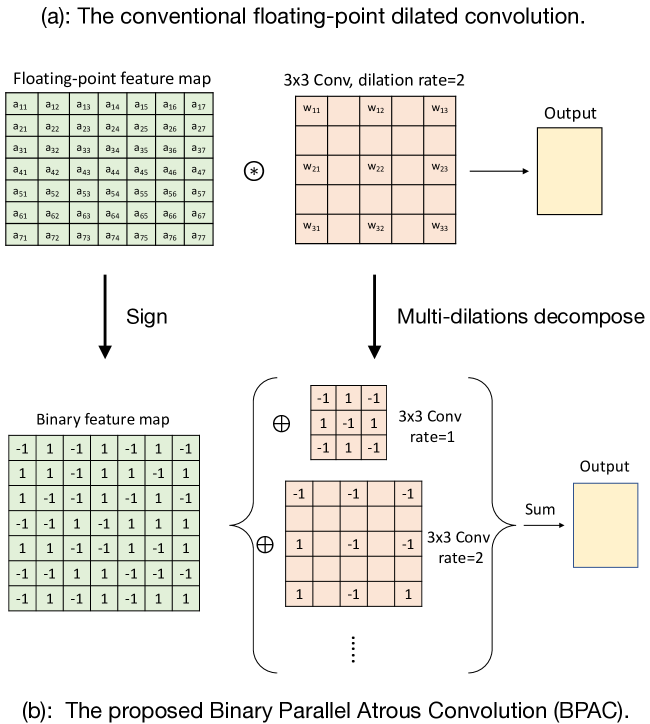
Figure 2: The comparison between conventional dilated convolution and BPAC. For expression convenience, the group only has one convolutional layer. $\circledast$ is the convolution operation and $\oplus$ indicates the XNOR-popcount operations. (a): The original floating-point dilated convolution. (b): We decompose the floating-point atrous convolution into a combination of binary bases, where each base uses a different dilated rate. We sum the output features of each binary branch as the final representation.

3.5 Extension to semantic segmentation

The key message conveyed in the proposed method is that, although each binary branch has a limited modeling capability, aggregating them together leads to a powerful model. In this section, we show that this principle can be applied to tasks other than image classification. In particular, we consider semantic segmentation which can be deemed as a dense pixel-wise classification problem. In the state-of-the-art semantic segmentation network, the atrous convolutional layer chen2017rethinking is an important building block, which performs convolution with a certain dilation rate. To directly apply the proposed method to such a layer, one can construct multiple binary atrous convolutional branches with the same structure and aggregate results from them. However, we choose not to do this but propose an alternative strategy: we use different dilation rates for each branch. In this way, the model can leverage multiscale information as a by-product of the network branch decomposition. It should be noted that this scheme does not incur any additional model parameters and computational complexity compared with the naive binary branch decomposition. The idea is illustrated in Figure 2 and we term this strategy Binary Parallel Atrous Convolution (BPAC).

In this work, we use the same ResNet backbone in chen2017rethinking ; chen2018encoder with output stride=8, where the last two stages employ atrous convolution. In BPAC, we keep $rates=\{2,...,K+1\}$ and $rates=\{6,...,K+5\}$ for $K$ bases in the last two blocks, respectively. Intriguingly, as will be shown in Section 5.3, our strategy brings so much benefit that using five binary bases with BPAC achieves similar performance as the original full precision network despite the fact that it saves considerable computational cost.

3.6 Extension to object detection

We further generalize GroupNet to the object detection task. We work on the one-stage detector, which consists of backbone, feature pyramid and heads. We directly use the backbone network pretrained on the ImageNet classification task to initialize the detection backbone. For the feature pyramid, it attaches a $1\times 1$ and $3\times 3$ convolutional layer at each resolution to adapt the feature maps. Since it lacks of structural information like the backbone network, we therefore apply the layer-wise binary decomposition in Section 3.2.1. Furthermore, the detection heads occupy a large portion of complexity in the whole detection framework. And each head is comprised of several consequent layers which is similar to a basic residual block. To preserve the structural information, following the spirit of group-wise binary decomposition strategy in Section 3.2.2, we propose to approximate each head as a whole. The structure is illustrated in Figure 3.

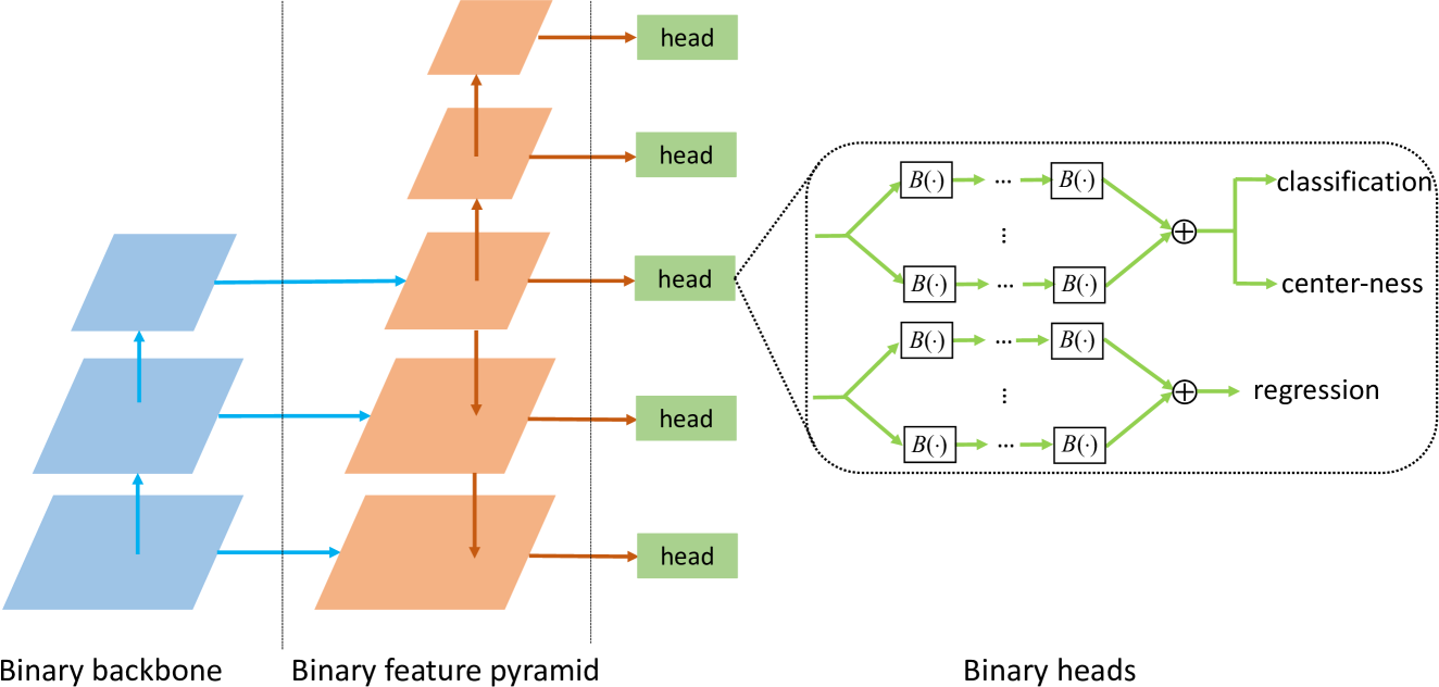
Figure 3: Illustration of the proposed binary detection framework. We partition the whole framework into three parts, namely, binary backbone, binary feature pyramid and binary heads.

We note that except the last layers for classification, center-ness and regression, other parameters of the heads are not shared across all feature pyramid levels which is the opposite of the full-precision counterpart. Such a design is motivated by the observation in chen2021aqd that there is a large divergence of activation distributions across different feature pyramid levels. To capture accurate batch statistics, we privatize BN layers for each pyramid level. Moreover, as a single binary convolutional layer has worse representational capability than the fixed-point one, we also use separate convolutional weights to ensure the model capacity. More optimization details are explained in Section 5.4.

4 Discussions

Differences from fixed-point quantization approaches. Our GroupNet is different from fixed-point quantization approaches zhang2018lq ; zhuang2018towards ; zhou2016dorefa ; mishra2018apprentice in both the quantization algorithm and its underlying inference implementation.

Note that in conventional fixed-point methods, the inner product between fixed-point weights and activations can be computed by bitwise operations. Let ${{\bf w}}\in{\mathbb{R}^{M}}$ and ${\bf a}\in{\mathbb{R}^{M}}$ be the weights and activations, respectively. they can be encoded by a linear combination of binary bases, respectively. In particular, ${\bf w}$ and ${\bf a}$ can be encoded by ${\bf{b}}_{i}^{w}\in{\{-1,1\}^{M}}$ and ${\bf{b}}_{i}^{a}\in{\{-1,1\}^{M}}$, where $i=1,...,P$, respectively. Let $Q_{P}(\cdot)$ be any quantization function, and for simplicity, we here consider uniform quantization only. Then, the inner product of ${\bf w}$ and ${\bf a}$ can be approximated by

$${Q_{P}}({{\bf{w}}^{\mathrm{T}}}){Q_{P}}({\bf{a}})=\sum\limits_{i=0}^{P-1}{\sum\limits_{j=0}^{P-1}{{2^{i+j}}}}({\bf{b}}_{i}^{w}\mathbin{\oplus}{\bf{b}}_{j}^{a}).$$ (11)

where $\mathbin{\oplus}$ indicates the binary inner product, which can be efficiently implemented by $\rm popcount$ and $\rm xnor$ bit-wise instructions that are commonly equipped in modern computers. According to Eq. (11), the computational complexity is $O(MP^{2})$ for the fixed-point inner product. Bearing the group-wise binary decomposition in Section 3.2 in mind, it can be easily realized that the proposed GroupNet with $K$ bases has the same computational complexity with the conventional $P$-bit fixed point quantization when $K=2^{P}$. However, compared with the $P$-bit fixed point quantization, the proposed GroupNet with $2^{P}$ bases introduces extra additions from the fusion of decomposition branches. It is worth noting that the convolution is implemented with two steps: $\rm im2col$ and $\rm GEMM$. The high-precision additions can be efficiently merged into the $\rm im2col$ operation of the succeeding layer during implementation. For $\rm im2col$ operation, most of the time is spend on data rearrangement, an extra tensor addition will have a very limited influence on its execution time. Moreover, the extra additions only account for a small portion of the overall network complexity, which intrinsically limits the impact on the overall speed. To justify our analysis, we provide speedup evaluations in Section 6.1. We also provide the analysis of the runtime training and inference memory cost in Section 6.2.

To emphasize, the proposed GroupNet enables much more flexible design of the quantization algorithm. Benefiting from the group-wise binary decomposition, the proposed GroupNet allows more fine-grained exploration space, where the quantization levels can be chosen from the continuous positive integer domain. In contrast, conventional fixed-point quantization requires the quantization levels to be the power of 2. For example, the bit-width of GroupNet with 5 bases is between 2-bit and 3-bit. Thus, GroupNet enjoys a flexible trade-off between complexity and accuracy by setting appropriate $K$. Moreover, as introduced in Section 3.5 and Section 3.6, our GroupNet is demonstrated to be more efficient in exploiting task-specific information or structures to compensate the quantization information loss.

Moreover, we define the model size of the full-precision model as $\Omega$. Then, the model size for GroupNet with $K$ bases becomes $K\Omega/32$ and the one for $P$-bit fixed-point quantization is $P\Omega/32$.

Based on the above analysis, we summarize that the proposed GroupNet introduces small additional run-time cost caused by the extra addition operations, however, provides benefits in algorithm flexibility and performance.

Differences between GroupNet and other multiple binarizations methods. In lin2017towards , a linear combination of binary weight/activations bases are obtained from the full-precision weights or activations without being directly learned. In contrast, we directly design the binary network structure, where binary weights are end-to-end optimized.  fromm2018heterogeneous ; tang2017train ; guo2017network ; li2017performance propose to recursively approximate the residual error and obtain a series of binary maps corresponding to different quantization scales. However, it is a sequential process which cannot be paralleled. Also, all previous multiple binarizations methods belong to local tensor approximation. In contrast to value approximation, we propose a group decomposition approach to approximate the full-precision network. Moreover, tensor-based methods are tightly designed to local value approximation and may be hardly generalized to other tasks accordingly. In addition, our group decomposition strategy achieves much better performance than tensor-level approximation as shown in Section 5.2.2.

5 Experiments

We define several methods for comparison as follows: GroupNet-A: It implements the full model with learnt soft connections described in Section 3.3. Following Bi-Real Net liu2020bi , we apply skip connection bypassing every binary convolution to improve the convergence. Note that due to the binary convolution, skip connections are high-precision which can be efficiently implemented using fixed-point addition. GroupNet-B: Based on GroupNet-A, we keep the $1\times 1$ downsampling skip connections to high-precision (i.e., 8-bit) similar to bethge2018training ; Liu_2018_ECCV . GroupNet-C: Based on GroupNet-B, we replace the soft routing mechanism with the dynamic hard gating. By default, we train 8 bases and dynamically select 4 bases during inference.

5.1 Evaluation on ImageNet

5.1.1 Experimental settings

Table 2: Performance comparisons of different binarization methods on ImageNet. We use operations count (OPs) to measure the computational cost. “-” denotes that the results are not reported. “W” and “A” refer to the weight and activation bitwidth respectively. We use the customized MobileNetV1 structure following ReActNet.

Network	Method	Bitwidth (W/A)	#Parameters (Mbit)	OPs ($\times 10^{8}$)	Top-1 Acc. (%)	Top-5 Acc. (%)
ResNet-18	Full-precision	32/32	374.0	18.17	69.7	89.4
2-7	BNNs hubara2016binarized	1/1	27.2	1.47	42.2	67.1
	XNOR-Net rastegari2016xnor	1/1	33.7	1.67	51.2	73.2
	Bi-RealNet Liu_2018_ECCV	1/1	33.6	1.63	56.4	79.5
	Real-to-Binary Net martinez2020training	1/1	44.6	1.83	65.4	86.2
	HCE bulat2021high	1/1	293.7	1.37	67.5	87.5
2-7	BitSplit kim2020algorithm	(1/1) $\times$ 4	-	2.47	58.4	80.6
	BENN zhu2019binary	(1/1) $\times$ 6	168.9	8.70	61.0	-
	Circulant CNN liu2019circulant	(1/1) $\times$ 4	-	2.47	61.4	82.8
2-7	GroupNet-A	(1/1) $\times$ 4	50.0	2.25	65.2	85.7
	GroupNet-B	(1/1) $\times$ 4	54.8	2.43	67.3	87.6
	GroupNet-C	(1/1) $\times$ 4	105.5	2.43	68.2	88.3
ResNet-34	Full-precision	32/32	697.5	36.68	73.2	91.4
2-7	Bi-RealNet Liu_2018_ECCV	1/1	43.8	1.93	62.2	83.9
	BENN zhu2019binary	(1/1) $\times$ 6	230.9	10.44	64.7	84.4
	GroupNet-A	(1/1) $\times$ 4	103.7	3.40	68.7	88.3
	GroupNet-B	(1/1) $\times$ 4	108.5	3.58	70.7	89.6
	GroupNet-C	(1/1) $\times$ 4	188.2	3.58	72.2	90.5
ResNet-50	Full-precision	32/32	817.8	41.00	76.0	92.9
2-7	Bi-RealNet Liu_2018_ECCV	1/1	176.8	5.36	62.6	83.9
	BENN zhu2019binary	(1/1) $\times$ 6	545.9	10.93	66.2	85.8
	GroupNet-A	(1/1) $\times$ 4	117.0	3.68	69.8	88.0
	GroupNet-B	(1/1) $\times$ 4	194.6	7.05	71.3	90.2
	GroupNet-C	(1/1) $\times$ 4	217.6	7.05	73.4	91.0
MobileNetV1	Full-precision	32/32	937.2	48.33	72.4	-
2-7	Bi-RealNet Liu_2018_ECCV	1/1	72.5	1.90	58.2	81.0
	ReActNet-C∗ liu2020reactnet	1/1	83.4	2.14	70.0	-
	BENN zhu2019binary	(1/1) $\times$ 6	370.5	5.32	63.0	84.0
	GroupNet-A	(1/1) $\times$ 4	124.0	3.19	66.8	86.2
	GroupNet-B	(1/1) $\times$ 4	133.8	4.16	70.8	89.5
	GroupNet-C	(1/1) $\times$ 4	259.3	4.16	72.1	90.3

• ^∗ denotes that we remove the knowledge distillation loss for fair comparison.

Dataset. The proposed method is first evaluated on ImageNet (ILSVRC2012) russakovsky2015imagenet dataset. ImageNet is a large-scale dataset which has $\sim$1.2M training images from 1K categories and 50K validation images. Several representative networks are tested: ResNet-18 he2016deep , ResNet-34, ResNet-50 and MobileNetV1 howard2017mobilenets . As discussed in Section 4, we compare the proposed approach with binary neural networks in Table 2 and fixed-point approaches in Table 3, respectively.

Implementation details. As in rastegari2016xnor ; Cai_2017_CVPR ; zhou2016dorefa ; zhuang2018towards , we binarize the weights and activations of all convolutional layers, except that the first and the last layers are quantized to 8-bit. In all ImageNet experiments, training images are resized to $256\times 256$, and a $224\times 224$ crop is randomly sampled from an image or its horizontal flip, with the per-pixel mean subtracted. We do not use any further data augmentation in our implementation. We use a simple single-crop testing for standard evaluation. No bias term is utilized. Following martinez2020training , training is divided into two stages. In the first stage, we train a network with binary activations and real-valued weights from scratch. In the second stage, we inherit the weights from the first step as the initial value and fine-tune the network with weights and activations both being binary. For both stages, we use the Adam optimizer with a linear learning rate decay scheduler, an initial learning rate of 5e-4 and a batch size of 256. We optimize the network for maximum 90 epochs in each stage. The weight decay is set to 1e-5 for the first stage and 0 for the second stage. Following Cai_2017_CVPR ; zhuang2018towards , no dropout is used due to binarization itself can be treated as a regularization. We initialize the dynamic hard gating parameters $\boldsymbol{\nu}$ using Kaiming initialization he2015delving and optimize them in conjunction with other network parameters using backpropagation. We apply layer-reordering to the networks as: $\rm Sign$ $\to$ $\rm Conv$ $\to$ $\rm PReLU$ $\to$ $\rm BN$. Inserting $\rm PReLU(\cdot)$ after convolution is important for convergence. We follow the BN folding literature jacob2017quantization ; chen2021aqd to fuse BN parameters into convolutional weights during inference. During training, the BN parameters and the convolutional weights are updated separately. Our simulation implementation is based on PyTorch paszke2017automatic .

OPs calculation. We follow the calculation method in martinez2020training , where we count the binary operations (BOPs) and floating point operations (FLOPs) separately. Then the total operations (OPs) is calculated by OPs = BOPs/64 + FLOPs, following the literature liu2020reactnet ; Liu_2018_ECCV ; rastegari2016xnor in BNNs.

Model size calculation. Following the common practise in the literature rastegari2016xnor ; Liu_2018_ECCV , the model size is calculated by $32\times N_{f}+P\times N_{P}+N_{b}$, where $N_{f}$, $N_{P}$ and $N_{b}$ are the number of full-precision, $P$-bit fixed-point and binary weights, respectively.

5.1.2 Comparison with binary neural networks

Since we employ binary weights and binary activations, we directly compare to the previous state-of-the-art binary approaches, including standard binary neural networks BNN hubara2016binarized , XNOR-Net rastegari2016xnor , Bi-RealNet Liu_2018_ECCV , ReActNet liu2020reactnet , Real-to-Binary Net martinez2020training , HCE bulat2021high ; and multiple binarization methods BitSplit kim2020algorithm , Circulant CNN liu2019circulant , BENN zhu2019binary . We report the results in Table 2 and summarize the following points. 1): When comparing with other multiple binarizations methods, our GroupNet shows better performance with comparable complexity. In comparison to directly binarizing networks, GroupNet also achieves better performance with moderate complexity increase. In summary, our approach achieves an improved trade-off between computational complexity and prediction accuracy. 2): We observe that GroupNet-B outperforms GroupNet-A by a large margin. It justifies keeping $1\times 1$ downsampling skip connections to high-precision is crucial for achieving high performance. 3): For Bottleneck structure in ResNet-50, we find larger quantization error than the counterparts using basic blocks with $3\times 3$ convolutions in ResNet-18 and ResNet-34. The similar observation is also found by bethge2018learning . We assume that this is mainly attributable to the $1\times 1$ convolutions in Bottleneck. The reason is $1\times 1$ filters are limited to two states only (either 1 or $-1$) and they have very limited learning power. Moreover, the bottleneck structure reduces the number of filters significantly, which implies the gradient paths are greatly reduced, leading to increased optimization difficulty.

5.1.3 Comparison with fixed-point approaches

Table 3: Performance comparisons of different methods on ImageNet. We use operations count (OPs) to measure the computational cost. “-” denotes that the results are not reported. “W” and “A” refer to the weight and activation bitwidth respectively.

Network	Method	Bitwidth (W/A)	#Parameters (Mbit)	OPs ($\times 10^{8}$)	Top-1 Acc. (%)	Top-5 Acc. (%)
ResNet-18	Full-precision	32/32	374.0	18.17	69.8	89.1
2-7	GroupNet-C	(1/1) $\times$ 4	105.5	2.43	68.2	88.3
	LSQ esser2020learned	2/2	61.6	2.25	67.6	87.6
	QIL jung2019learning	2/2	61.6	2.25	65.7	-
	PACT choi2018pact	2/2	61.6	2.25	64.4	-
	LQ-Net zhang2018lq	2/2	61.6	2.25	64.9	85.9
ResNet-34	Full-precision	32/32	697.5	36.68	73.3	91.4
2-7	GroupNet-C	(1/1) $\times$ 4	188.2	3.58	72.2	90.5
	LSQ esser2020learned	2/2	102.3	3.40	71.6	90.3
	QIL jung2019learning	2/2	102.3	3.40	70.6	-
	PACT choi2018pact	2/2	102.3	3.40	-	-
	LQ-Net zhang2018lq	2/2	102.3	3.40	69.8	89.1

Table 4: Performance of GroupNet and the width multiplier on ImageNet.

Model	Top-1 %	Top-5 %
GroupNet-A	65.2	85.7
Width multiplier	63.5	85.2

Table 5: Comparisons between several group-wise decomposition strategies. Top-1 and Top-5 accuracy (%) gaps to the corresponding full-precision ResNet-18 network are also reported.

Model	Bases	Top-1	Top-5	Top-1 gap	Top-5 gap
Full-precision	1	69.7	89.4	-	-
GroupNet-A	4	65.2	85.7	4.5	3.7
GBD v1	4	63.7	85.2	6.0	4.2
GBD v2	4	62.9	84.7	6.8	4.7
GBD v3	4	59.8	82.7	9.9	6.7
LBD	4	57.8	80.1	11.9	9.3

Since we use $K$ binary group bases, we compare our approach with at least $\sqrt{K}$-bit fixed-point approaches. In Table 3, we compare our approach with the state-of-the-art fixed-point approaches LSQ esser2020learned , QIL jung2019learning , PACT choi2018pact and LQ-Nets zhang2018lq .

All the comparison results are directly cited from the corresponding papers. From the results, we observe that with comparable computational complexity, the proposed GroupNet surpasses the state-of-the-art fixed-point methods, which demonstrates the flexibility and effectiveness of our method.

5.1.4 Extension on MobileNetV1

We further propose to apply GroupNet based on ReActNet. Specifically, ReActNet customizes the MobileNetV1 structure as the binarization backbone and GroupNet-C treats the ReActNet as the base structure. Following ReActNet, we make three modifications. 1): The $3\times 3$ depth-wise and the $1\times 1$ point-wise convolutional blocks in the MobileNetV1 are replaced by the $3\times 3$ and $1\times 1$ vanilla convolutions in parallel with shortcuts respectively. 2): For the reduction block, we duplicate the input activation and concatenate two blocks with the same inputs to address the channel number difference, permitting to add identity skip connections. 3): We also replace $\rm Sign$ and $\rm ReLU$ to $\rm RSign$ and $\rm RPReLU$ following ReActNet, respectively.

The empirical results show that our GroupNet is complementary to high-performance binary architectures ($K=1$) by exploring how to ensemble the binary bases ($K>1$) effectively to approximate the original full-precision network. Based on an advanced binary base architecture, our GroupNet can achieve better performance.

5.2 Ablation study on ImageNet classification

5.2.1 Width multiplier vs. structured approximation

We further compare the “structured approximation” with the width multiplier baseline howard2017mobilenets , which simply multiplies the channel number by a fixed ratio. To make the two settings directly comparable, we set $K=4$ and the width multiplier to 2. The results are shown in Table 4.

We observe that GroupNet outperforms the width multiplier baseline on ResNet-18. This further justifies the group-wise approximation can better preserve the information.

5.2.2 Effect of the group space

To show the importance of the space design, we define more methods for comparison as follows: LBD: It implements the layer-wise binary decomposition strategy described in Section 3.2.1. GBD v1: We implement with the group-wise binary decomposition strategy, where each base consists of one block. It corresponds to the approach described in Eq. (5) and is illustrated in Figure 1 (d). GBD v2: Similar to GBD v1, the only difference is that each group base has two blocks. It is illustrated in Figure 1 (e) and is explained in Eq. (6). GBD v3: It is an extreme case where each base is a whole network, which can be treated as an ensemble of a set of binary networks.  We present the results in Table 5.

From the results, we have two main observations and analysis. 1): The group-wise decomposition strategies (GBD v1-v3, GroupNet-A) outperform the layer-wise counterpart (LBD) by a large margin. Our speculation is that skip connections have been demonstrated to play an important role in increasing representational capability and improving gradient backpropagation in BNNs literature Liu_2018_ECCV . In this sense, group-wise variants have $K$ times more skip connections than LBD, which explains to some extent why the group-wise approximation performs much better. 2): As shown in product quantization jegou2011product , a fine quantization granularity is theoretically guaranteed to reduce the approximation error. Therefore, approximating one block as a whole is able to achieve the best trade-off since it simultaneously keeps the most skip connections at the fine granularity. This is reflected by the empirical results that the block-wise approximation (e.g., GroupNet-A and GBD v1) achieves the highest accuracy.

5.2.3 Effect of the number of bases

Table 6: Validation accuracy (%) of Group-Net on ImageNet with different number of bases. All cases are based on the ResNet-18 network with binary weights and activations.

Model	Bases	Top-1	Top-5	Top-1 gap	Top-5 gap
Full-precision	1	69.7	89.4	-	-
GroupNet-A	1	58.1	80.8	11.6	8.6
GroupNet-A	3	63.8	84.9	5.9	4.5
GroupNet-A	4	65.2	85.7	4.5	3.7
GroupNet-A	5	66.0	86.2	3.7	3.2

We further explore the influence of number of bases $K$ to the final performance in Table 6. When the number is set to 1, it corresponds to directly binarize the original full-precision network and we observe apparent accuracy drop compared to its full-precision counterpart. With more bases employed, we can find the performance steadily increases. The reason can be attributed to the better approximation of the floating-point network, which is a trade-off between accuracy and complexity. It can be expected that with enough bases, the network should has the capacity to approximate the full-precision network precisely.

5.2.4 Effect of the soft gate

Table 7: The effect of soft gates on ImageNet.

Model		Full	GroupNet-A (w/o softgates)	GroupNet-A
ResNet-18	Top-1 %	69.7	64.1	65.2
	Top-5 %	89.4	85.0	85.7
ResNet-34	Top-1 %	73.2	66.4	68.7
	Top-5 %	91.4	86.2	88.3
ResNet-50	Top-1 %	76.0	67.7	69.8
	Top-5 %	92.9	86.7	88.0

In this section, we further analysis the effect of soft gate described in Section 3.3.1. We show the quantitative results in Table 7. From the results, we can observe consistent accuracy improvement for various architectures. This shows that increasing the gradient paths and learning the information flow within BNNs is important for maintaining the performance. For instance, on ResNet-34, learning the soft gates can improve the Top-1 accuracy by $2.1\%$.

5.3 Evaluation on semantic segmentation

In this section, we further evaluate GroupNet on the PASCAL VOC 2012 semantic segmentation benchmark everingham2010pascal which contains 20 foreground object classes and one background class. The original dataset contains 1,464 (train), 1,449 (val) and 1,456 (test) images. The dataset is augmented by the extra annotations from hariharan2011semantic , resulting in 10,582 training images. The performance is measured in terms of averaged pixel intersection-over-union (mIOU) over 21 classes.

Implementation details. Our experiments are based on FCN long2015fully , where we adjust the dilation rates of the last two stages in ResNet with atrous convolution to make the output stride equal to 8. We empirically set dilation rates to be (4, 8) in last two stages. Similar to the structure of FCN-32s and FCN-16s, we define our modified baselines as FCN-8s-C5 and FCN-8s-C4C5, where C4 and C5 denote extracting features from the final convolutional layer of the 4-th and 5-th stage, respectively. We first pretrain the binary backbone on ImageNet dataset and fine-tune it on PASCAL VOC. During fine-tuning, we use Adam with initial learning rate=1e-4, weight decay=0 and batch size=16. We set the number of bases $K=4$ in experiments. We train 40 epochs in total and decay the learning rate by a factor of 10 at 20 and 30 epochs. We do not add any auxiliary loss and ASPP.

5.3.1 Experiments on FCN

Table 8: Performance of GroupNet on the PASCAL VOC 2012 validation set with FCN.

Backbone	Model	mIOU	$\Delta$
ResNet-18, FCN-8s-C5	Full-precision	64.9	-
	LSQ (2-bit)	60.8	4.1
	GroupNet-C	61.5	3.4
ResNet-18, FCN-8s-C4C5	Full-precision	67.3	-
	LSQ (2-bit)	62.9	4.4
	GroupNet-C	63.6	3.7
ResNet-34, FCN-8s-C5	Full-precision	72.7	-
	LSQ (2-bit)	68.5	4.2
	GroupNet-C	69.3	3.4
ResNet-50, FCN-8s-C5	Full-precision	73.1	-
	LSQ (2-bit)	69.6	3.5
	GroupNet-C	70.0	3.1

Table 9: Performance of GroupNet-C with BPAC on PASCAL VOC 2012 validation set with FCN.

Backbone	Model	mIOU
ResNet-18, FCN-8s-C5	Full-precision (multi-dilations)	67.6
	LSQ (2-bit)	64.0
	GroupNet-C + BPAC	66.2
ResNet-18, FCN-8s-C4C5	Full-precision (multi-dilations)	70.1
	LSQ (2-bit)	66.5
	GroupNet-C + BPAC	69.0
ResNet-34, FCN-8s-C5	Full-precision (multi-dilations)	75.0
	LSQ (2-bit)	71.3
	GroupNet-C + BPAC	73.9
ResNet-50, FCN-8s-C5	Full-precision (multi-dilations)	75.5
	LSQ (2-bit)	72.6
	GroupNet-C + BPAC	74.4

The main results are reported in Table 8 and Table 9. From the results in Table 8, we can observe that when all bases using the same dilation rate, there is an obvious performance gap with the full-precision counterpart. This performance drop is consistent with the classification results on ImageNet dataset in Table 3. It proves that the quality of extracted features has a great impact on the segmentation performance. Moreover, we also quantize the network to 2-bit using the state-of-the-art fixed-point quantization method LSQ. Compared with LSQ, we achieve better performance with comparable computational cost.

To reduce performance loss, we further employ diverse dilated rates on parallel binary bases to capture the multi-scale information without increasing any computational complexity. This formulates our final approach GroupNet-C + BPAC in Table 9, which shows significant improvement over the GroupNet-C counterpart. Moreover, the performance of GroupNet-C + BPAC outperforms the full-precision baseline in Table 8, which strongly justifies the flexibility of GroupNet.

5.3.2 Experiments on DeepLabv3

For training the DeepLabv3 chen2017rethinking baseline, we use Adam as the optimizer. The initial learning rate for training backbone network is set to 1e-4, and is multiplied by 10 for ASPP module. Similar to image classification, we keep the first layer and last classification layer to 8-bit. We employ the layer-wise approximation in quantizing the ASPP module. We set $K=4$ for both backbone and ASPP. The training details are the same with those in FCN except that we use the polynomial decay of learning rate. The results are provided in Table 11.

Moreover, a problem still exists in training binary DeepLabv3. The ASPP module uses large dilation rates for the three $3\times 3$ convolutions with $rates=\{12,24,36\}$ when output_stride=8. For training BNNs with Eq. (2), we apply one-paddings to constrain activations to $\{-1,1\}$. However, for atrous convolution with large rates, padding ones can introduce high bias and make the optimization difficult. To solve this problem, we instead binarize the activations to $\{0,1\}$ following the quantizer in zhou2016dorefa . Note that the numerical difference is only a scalar whether activations are represented by $\{-1,1\}$ or $\{0,1\}$ in bitwise operations to accelerate the dot products zhou2016dorefa ; zhang2018lq . The importance for binarizing activations to $\{0,1\}$ is shown in Table 10.

Table 10: The difference for binarizing ASPP with $\{-1,1\}$ and $\{0,1\}$. The metric is mIOU.

Model	full-precision	$\{0,1\}$	$\{-1,1\}$
ResNet-18	72.1	64.0	51.6

It is worth noting that the comparable counterpart of DeepLabv3 is the GroupNet-C + BPAC with FCN-8s-C5 in Table 9. The main difference is that in the proposed BPAC module, we directly incorporate the multiple dilation rates in the backbone network to capture multi-scale context. In contrast, DeepLabv3 embeds the ASPP module on top of the backbone network. With the same output_stride, the computational complexity of FCN is lower than DeepLabv3 since no additional ASPP is needed. With the simpler quantized FCN framework with BPAC, we can achieve comparable or even better performance than quantized DeepLabv3. For example, with the ResNet-34 backbone, GroupNet-C + BPAC outperforms DeepLabv3 by 5.9 w.r.t.  mIOU. It also shows that binarization on ASPP is sensitive to the final performance, since the binarization process constrains the feature magnitude to $\{0,1\}$ which causes the multi-scale information loss.

Table 11: Performance on the PASCAL VOC 2012 validation set with DeepLabv3.

Backbone	Model	mIOU	$\Delta$
ResNet-18	Full-precision	72.1	-
	Backbone	68.6	3.5
	Backbone + ASPP	65.0	7.1
ResNet-34	Full-precision	74.4	-
	Backbone	71.9	2.5
	Backbone + ASPP	68.0	6.4
ResNet-50	Full-precision	76.9	-
	Backbone	73.6	3.3
	Backbone + ASPP	70.2	6.7

5.4 Evaluation on object detection

In this section, we evaluate GroupNet on the general object detection task. Our experiments are conducted on the large-scale detection benchmark COCO lin2014microsoft . Following lin2017feature ; lin2017focal , we use the COCO trainval35k split (115K images) for training and minival split (5K images) for validation. We also report our results on the test_dev split (20K images) by uploading our detection results to the evaluation server. Our experiments are based on FCOS tian2019fcos and RetinaNet lin2017focal . In all settings, we set $K=4$.

Implementation details. In specific, the backbone is initialized by the pretrained weights on ImageNet classification. GroupNet is then fine-tuned with Adam with the initial learning rate of 5e-4 and the batch size of 16 for 90,000 iterations. The learning rate is decayed by 10 at iteration 60,000 and 80,000, respectively. Note that we keep updating the BN layers rather than fix them during training. Other hyper-parameters are kept the same with tian2019fcos ; lin2017focal .

5.4.1 Performance evaluation

Table 12: Performance on COCO validation set with different binarized components.

Model	AP	AP50	AP75	APS	APM	APL
Full-precision	33.8	51.8	36.1	19.3	36.4	44.4
Backbone	33.7	51.6	36.2	19.0	36.3	44.5
Backbone + Pyramid	32.9	50.3	35.7	18.8	35.1	42.8
Backbone + Pyramid + Heads (shared)	19.3	36.6	18.4	10.5	23.0	28.8
Backbone + Pyramid + Heads (w/o shared)	30.1	47.5	33.2	16.0	31.2	39.2

We report the performance on FCOS in Tables 13 and 14, as well as RetinaNet in Table 15, respectively. We can observe that GroupNet achieves promising results over all ResNet architectures. For instance, with the ResNet-18 backbone, the gap of AP is only 3.7 on FCOS while we save considerable computational complexity. This strongly shows that the proposed GroupNet is a general approach that can be extended on many fundamental computer vision tasks. Furthermore, we highlight that we are among the pioneering approaches to explore binary neural networks on object detection in the literature.

We compare with the state-of-the-art quantized object detector FQN li2019fully , and also quantize the detector with LQ-Net using the proposed training strategy. We observe that GroupNet-C outperforms the two comparing methods. It shows that learning independent heads is more effective than freezing batch normalization layers in FQN to stabilize the optimization. Moreover, the better low-precision feature quality of GroupNet also contributes to superiority of the performance.

Table 13: Performance on the COCO validation set based on FCOS.

Backbone	Model	#Parameters (Mbit)	FLOPs ($\times 10^{10}$)	AP	AP50	AP75	APS	APM	APL
ResNet-18	Full-precision	617.4	15.5	33.8	51.8	36.1	19.3	36.4	44.4
	FQN	86.2	1.01	26.2	43.5	26.7	13.3	29.5	35.7
	LQ-Net	86.2	1.01	28.0	45.0	30.6	15.0	29.8	36.6
	GroupNet-C	165.0	1.03	30.1	47.5	33.2	16.0	31.2	39.2
ResNet-34	Full-precision	940.8	19.3	37.5	55.9	40.3	22.6	40.8	47.4
	FQN	124.5	1.25	28.8	46.3	30.0	14.8	31.0	38.8
	LQ-Net	124.5	1.25	30.8	47.8	33.4	16.2	32.5	40.0
	GroupNet-C	245.8	1.27	32.8	49.8	35.6	17.4	34.0	41.8
ResNet-50	Full-precision	1034.0	20.4	38.6	57.4	41.4	22.3	42.5	49.8
	FQN	137.2	1.32	29.7	47.1	30.8	15.3	31.8	39.3
	LQ-Net	137.2	1.32	32.1	49.6	34.8	17.6	33.2	40.6
	GroupNet-C	260.4	1.64	33.9	51.2	37.3	18.3	35.0	42.5

Table 14: Performance on the COCO test set based on FCOS.

Backbone	Model	AP	AP50	AP75	APS	APM	APL
ResNet-18	Full-precision	33.9	51.9	36.4	19.4	35.6	42.2
	FQN	26.3	43.8	26.8	13.5	29.4	35.4
	LQ-Net	28.2	45.3	30.7	15.1	29.6	36.1
	GroupNet-C	30.2	47.7	33.3	15.9	31.4	39.4
ResNet-34	Full-precision	37.8	56.3	41.0	22.1	40.1	46.7
	FQN	28.9	46.6	30.1	14.5	31.5	37.8
	LQ-Net	30.9	47.5	33.5	16.0	32.3	39.5
	GroupNet-C	32.6	49.4	35.7	17.3	34.2	41.7
ResNet-50	Full-precision	38.8	57.9	41.9	22.4	41.5	48.0
	FQN	29.9	47.4	31.0	14.9	31.7	39.0
	LQ-Net	32.0	49.5	35.1	17.4	32.7	40.0
	GroupNet-C	33.8	51.4	37.5	18.0	35.1	42.4

Table 15: Performance on the COCO validation set based on RetinaNet.

Backbone	Model	#Parameters (Mbit)	FLOPs ($\times 10^{10}$)	AP	AP50	AP75	APS	APM	APL
ResNet-18	Full-precision	685.8	18.8	32.9	52.7	34.8	19.8	35.6	41.7
	FQN (2-bit)	135.7	1.43	28.2	46.5	29.2	15.6	30.0	37.7
	GroupNet-C	182.1	1.44	30.7	48.0	32.8	16.4	32.2	39.8
ResNet-34	Full-precision	1008.6	22.6	36.2	56.6	38.7	22.1	39.6	45.1
	FQN (2-bit)	175.8	1.66	31.5	50.4	33.2	17.1	34.3	41.4
	GroupNet-C	262.4	1.68	33.4	52.1	36.4	18.0	35.2	42.5
ResNet-50	Full-precision	1215.6	23.9	37.8	58.5	40.7	22.8	41.3	48.3
	FQN (2-bit)	203.1	1.74	31.9	51.1	33.5	17.9	35.1	40.3
	GroupNet-C	305.7	2.06	34.2	52.5	37.5	18.9	35.6	43.3

5.4.2 Detection components analysis

We further analysis the affect of quantizing the backbone, feature pyramid and heads to the final performance, respectively. The results are reported in Table 12.

From Table 12, binarizing the backbone and the feature pyramid only downgrades the performance by a small margin. However, binarizing heads causes an obvious AP drop. It can be attributed to that heads are responsible for adapting the extracted multi-level features to the classification and regression objectives. As a result, its representability is crucial for robust detectors. However, the multi-level information is undermined when being constrained to $\{-1,1\}$. This shows that the detection modules other than the backbone are sensitive to quantization, and we leave it as our future work.

By comparing the results with respect to weight sharing, we observe the original sharing heads strategy that widely used in full-precision detection frameworks performs extremely bad in the binary setting. In specific, with ResNet-18 backbone, the AP gap between with and without weight sharing reaches by 10.8. It is worth noting that separating the parameters does not increase any additional computational complexity. Even though the number of parameters are increased (i.e., by $\sim 4$ times in heads), the memory consumption is still significantly reduced due to the 1-bit storage.

6 Acceleration on hardware

Figure 4: Example code to implement binary GEMM with GPU instructions. The following kernel will be executed in SIMD (single instruction, multiple data stream) manner on the GPU.

⬇

__kernel void gemm_v1(

__global half *dst, // GEMM result buffer, in dimension of [M * N]

__global uchar *src, // activation, in dimension of [M * K]

__global uchar *weight, // weight parameters, in dimension of [N, K]

__global half *bias, // bias parameters

int M, int N, int K,

half alpha // quantization scale factor

)

{

int x = get_global_id(0); // thread id

int y = get_global_id(1); // thread id

x = min(x, M-1);

y = min(y, N-1);

uchar buffer;

uchar filter;

short result;

result = 0;

short i;

for(i=0; i<K; i++) {

buffer = src[i*M + x];

filter = weight[i*N + y];

result += popcount(buffer ^ filter); // obtain count of ones

}

result = (short)(K*8) - result * (short)2; // obtain binary inner product result

half save;

save = result * alpha;

dst[y*M + x] = save + bias[y];

return;

}

Table 16: The execution time (us) of a single layer with different configurations.

Device	model	case1	case2	case3	case4	case5	case6	case7	case8	case9	case10	case11
Qualcomm 821	2-bit	1928	3543	7968	24914	93069	1512	2348	3546	7188	21187	75486
	GroupNet	2014	3621	8163	25376	94550	1613	2487	3627	7311	21362	75982
2-13	Relative	4.4%	2.2%	2.4%	1.8%	1.6%	6.6%	5.9%	2.3%	1.7%	0.8%	0.7%
Qualcomm 835	2-bit	2076	2969	6463	20528	73967	1600	1900	2852	5646	15822	69803
	GroupNet	2255	3206	6930	21776	75010	1754	1998	2982	5746	17676	71140
2-13	Relative	8.6%	8.0%	7.2%	6.1%	1.4%	9.6%	5.1%	4.6%	1.8%	11.7%	1.9%
Kirin 970	2-bit	900	2234	2544	8040	31027	1048	1594	2415	2390	6750	24087
	GroupNet	1017	2603	2550	8030	31145	1060	1594	2535	2478	6764	24326
2-13	Relative	13.0%	16.5%	0.2%	-0.1%	0.4%	1.1%	0.0%	5.0%	3.7%	0.2%	1.0%

Table 17: Exact execution time ($\rm ms$) and speedup ratios for overall quantized layers. We run 5 times and report the results with mean and standard deviation.

Device	Network	Binary	GroupNet-C	2-bit	Binary vs. GroupNet-C	Binary vs. 2-bit	GroupNet-C vs. 2-bit
Q835	ResNet-18	12.1$\pm$0.2	48.8$\pm$0.3	44.8$\pm$0.2	4.03	3.70	0.92
	ResNet-34	25.3$\pm$0.3	98.0$\pm$0.5	90.6$\pm$0.4	3.87	3.58	0.93
Q821	ResNet-18	15.7$\pm$0.3	55.4$\pm$1.6	52.5$\pm$1.0	3.45	3.34	0.95
	ResNet-34	32.3$\pm$0.6	110.3$\pm$2.6	105.2$\pm$2.1	3.41	3.26	0.95

To investigate the real execution speed and memory cost of the proposed GroupNet and other related counterparts such as fixed-point quantization, we develop the acceleration code (GPU version only) on resource constrained platforms and provide the benchmark results. Experimental platforms include HiSilicon Kirin 970, Qualcomm 821 as well as Qualcomm 835. For fair comparison, we fix the frequency of the sub-systems (such as the CPU, GPU and DDR) if possible in order to prevent interference from the DVFS (dynamic voltage and frequency scaling) on the modern operating system. We fuse the batch normalization layers into the corresponding convolutional layers following jacob2017quantization ; chen2021aqd . Multiple rounds of experiments are conducted and the profiling data is averaged for statistic stability.

6.1 Execution speed benchmarks

Implementation details. We employ OpenCL (similar with CUDA and is a common programming language on the embedded platforms) to implement the GPU acceleration. Arithmetic and bit-wise logical operations, such as $\rm popcount$ and $\rm xor$ are supported in the OpenCL language. Dedicated software is developed for the proposed neural network acceleration. As explained in Sec. 4, the binary convolution is implemented with two steps: $\rm im2col$ and $\rm GEMM$. We provide the example implementation in Figure 4.

Results analysis. We first compare the layer-wise execution time between GroupNet (refer to Eq. (3)) with 4 bases and 2-bit models. The results are listed in Table 16. A total of 11 cases are included in this experiment. All cases are with convolutions of $3\times 3$ kernel, padding 1 and stride 1. For convenience, we configure the input and output feature maps to have the same shape, where input channels/width/height = output channels/width/height, respectively. For the first five cases, we fix the channel number to be 64 and increase the resolution from 28 to 448 with a multiplier 2. For the last six cases, we fix the resolution to be $56\times 56$ and double the channel number from 16 to 512. From the results, we observe that the inference speed of GroupNet is slighter slower than that of the $2$-bit model due to the extra addition operations discussed in Section 4. We set the batch size to 1 in all scenarios. We also report the overall speed for all quantized layers in Table 17 of BNNs, GroupNet-C (4 bases) and 2-bit models. From Table 17, we first observe that the real execution time of GroupNet-C and 2-bit models is less than $4\times$ slower than the binary case. Moreover, we also report the speedup of the 4 bases GroupNet-C against the $2$-bit model. Specifically, the relative speedup ranges from 0.92 to 0.95 across different architectures (ResNet-18 and ResNet-34) on various devices (Qualcomm 821 and 835). It implies the extra addition operations analyzed in Section 4 has small impact on the overall inference speed. In summary, the group-wise approximation is still hardware-friendly but more flexible and accurate.

We finally report the inference time of binary convolutions and high-precision additions respectively in Table 18, where we can observe that “hAdd” executes much faster than “bConv”.

Table 18: Comparison on the inference time of the binary convolution and high-precision addition. ‘bConv’ and ‘hAdd’ indicate the binary convolution and the high-precision addition, respectively.

Device	Mode	case1	case2	case3	case4	case5	case6	case7	case8	case9	case10	case11
Qualcomm 821	bConv	588	1227	2634	8265	31106	476	737	1249	2259	6000	19914
	hAdd	191	510	832	1769	5592	187	366	510	677	1038	1311
Qualcomm 835	bConv	652	918	1915	6053	23718	526	692	946	1790	4839	17394
	hAdd	98	209	375	1051	3899	114	122	210	262	362	577
Kirin 970	bConv	337	742	849	2617	9762	317	465	698	693	1898	6292
	hAdd	73	113	272	957	3811	107	113	162	219	333	522

Table 19: Memory consumption ($\rm MB$) with ResNet-18 for the proposed method and fixed-point quantization scheme. For memory during training, we set the training batch size to be 64 and measure the GPU memory cost. For storage needed in the inference mode, we report the consumption by the activations and weights, respectively, in a format of ‘a + w’ (we do not include the memory consumption of the input layer and the output layer).

Mode	GroupNet-C			Fixed-point
	base			a/w
	2	3	4	1/1	2/2	4/4	FP32/FP32
training	3953	5117	6275	4969	4969	4969	-
inference	2.06 + 4.59	2.06 + 6.89	2.06 + 9.18	1.43 + 2.30	1.65 + 4.59	2.11 + 9.18	9.70 + 73.44

6.2 Runtime memory consumption

We further explore the actual training and inference memory consumption of GroupNet-C and the fixed-point quantization scheme. Note that we focus more on the runtime memory footprint in practice because energy consumption is dominated by memory access han2016deep . We measure the runtime memory consumption with ResNet-18 on ImageNet, as illustrated in Table 19.

Implementation details. When developing the acceleration code with OpenCL on the target platforms, we find the memory allocation is quite time consuming. Therefore, we leverage the compilation phase allocation strategy. Specifically, we build up the computation graph for the network inference and record the lifetime of each tensor. Only one static memory pool is allocated, where tensors are mapped into sub-buffers of this memory pool. When the lifetime of a tensor ends, the buffer is marked free and can be re-used by the following tensors. The mapping pattern is pre-determined at the compilation stage and hard-coded into the program, thus negligible time is introduced by the memory mapping during runtime.

Results analysis. In the training phase, we use “fake quantization”, where we simulate the quantization by rounding the tensors into binary ones, however still represent the data with floating-point. Each extra branch would introduce an extra memory cost (memory can not be re-used among different branches, as the tensors are saved for back-propagation). Thus, the training memory increases linearly with the number of bases $K$ in GroupNet. In contrast, the fixed-point solution has a fixed amount of memory consumption for all bit quantization training ($K=1$).

For the runtime memory footprint at the testing time, we count the activation storage and weight storage separately. In particular, the activation storage of our GroupNet only brings a fixed amount of memory cost. It is because after the computation of each branch, the buffer is freed and re-used in the next branch. Specifically, a memory pool is allocated with the capacity being dependent by the largest buffer in the network. In practice, we found the largest buffer is occupied by the $\rm im2col$ result of the input convolutional layer (this layer has a large kernel size of $\rm 7\times 7$) for ResNet. However, for the fixed-point quantization scheme, the activation memory consumption increases with the bitwidth configuration. In other words, a fixed-point method needs to be pre-allocated memory for $P$-bit while GroupNet only needs a buffer for 1-bit (1 base). Note that accumulation is required for our GroupNet, which might not be freed when handling different branches. As a result, the preliminary size of the memory pool of our GroupNet ($2.06$ MB) is generally larger than that of the fixed-point solution ($1.43$ MB for $1/1$).

Moreover, for weight parameters storage during inference, the memory consumption is directly decided by the base number $K$ or quantization bitwidth.

In summary, under comparable FLOPs, GroupNet-C (base $=4$) consumes higher runtime memory footprint than 2-bit fixed-point models, i.e., 11.24 MB vs. 6.24MB, where both are much less than the full-precision one, 83.14MB. The gap mainly comes from storing more parameters in our GroupNet.

7 Conclusion

In this paper, we have explored highly efficient and accurate CNN architectures with binary weights and activations. Specifically, we have proposed to directly decompose the full-precision network into multiple groups and each group is approximated using a set of binary bases which can be optimized in an end-to-end manner. We have also proposed to learn the decomposition automatically. To increase model capacity, we have introduced conditional computing to binary networks, where the bases in each group are dynamically executed. Experimental results have proved the effectiveness of the proposed approach on the ImageNet classification task. More importantly, we have generalized the proposed GroupNet approach from image classification tasks to more challenging fundamental computer vision tasks, namely dense prediction tasks such as semantic segmentation and object detection. We highlight that we may be among the first few approaches to apply binary neural networks on general semantic segmentation and object detection tasks, and achieve encouraging performance on the PASCAL VOC and COCO datasets with binary networks. Last, we have developed the underlying acceleration code and speedup evaluation comparing with other quantization strategies is analyzed on several platforms, which serves as a strong benchmark for further research. In the future, we will employ the latent-free optimizer helwegen2019latent for BNNs that directly update the binary weights, to reduce the memory consumption during training. We will also develop acceleration code on X86, ARMs and FPGA platforms.

References

- (1) K. He, X. Zhang, S. Ren, and J. Sun, “Deep residual learning for image recognition,” in Proc. IEEE Conf. Comp. Vis. Patt. Recogn., 2016, pp. 770–778.
- (2) J. Long, E. Shelhamer, and T. Darrell, “Fully convolutional networks for semantic segmentation,” in Proc. IEEE Conf. Comp. Vis. Patt. Recogn., 2015, pp. 3431–3440.
- (3) L.-C. Chen, Y. Zhu, G. Papandreou, F. Schroff, and H. Adam, “Encoder-decoder with atrous separable convolution for semantic image segmentation,” in Proc. Eur. Conf. Comp. Vis., 2018, pp. 801–818.
- (4) Z. Tian, C. Shen, H. Chen, and T. He, “Fcos: Fully convolutional one-stage object detection,” in Proc. IEEE Int. Conf. Comp. Vis., 2019.
- (5) Z. Zhuang, M. Tan, B. Zhuang, J. Liu, Y. Guo, Q. Wu, J. Huang, and J. Zhu, “Discrimination-aware channel pruning for deep neural networks,” in Proc. Adv. Neural Inf. Process. Syst., 2018, pp. 883–894.
- (6) Y. He, X. Zhang, and J. Sun, “Channel pruning for accelerating very deep neural networks,” in Proc. IEEE Int. Conf. Comp. Vis., vol. 2, 2017, p. 6.
- (7) S. Lin, R. Ji, C. Yan, B. Zhang, L. Cao, Q. Ye, F. Huang, and D. Doermann, “Towards optimal structured cnn pruning via generative adversarial learning,” in Proc. IEEE Conf. Comp. Vis. Patt. Recogn., 2019, pp. 2790–2799.
- (8) B. Zhuang, C. Shen, M. Tan, L. Liu, and I. Reid, “Towards effective low-bitwidth convolutional neural networks,” in Proc. IEEE Conf. Comp. Vis. Patt. Recogn., 2018, pp. 7920–7928.
- (9) B. Jacob, S. Kligys, B. Chen, M. Zhu, M. Tang, A. Howard, H. Adam, and D. Kalenichenko, “Quantization and training of neural networks for efficient integer-arithmetic-only inference,” in Proc. IEEE Conf. Comp. Vis. Patt. Recogn., 2018.
- (10) F. Chollet, “Xception: Deep learning with depthwise separable convolutions,” in Proc. IEEE Conf. Comp. Vis. Patt. Recogn., 2017, pp. 1251–1258.
- (11) A. G. Howard, M. Zhu, B. Chen, D. Kalenichenko, W. Wang, T. Weyand, M. Andreetto, and H. Adam, “Mobilenets: Efficient convolutional neural networks for mobile vision applications,” arXiv preprint arXiv:1704.04861, 2017.
- (12) I. Hubara, M. Courbariaux, D. Soudry, R. El-Yaniv, and Y. Bengio, “Binarized neural networks,” in Proc. Adv. Neural Inf. Process. Syst., 2016, pp. 4107–4115.
- (13) M. Rastegari, V. Ordonez, J. Redmon, and A. Farhadi, “Xnor-net: Imagenet classification using binary convolutional neural networks,” in Proc. Eur. Conf. Comp. Vis., 2016, pp. 525–542.
- (14) A. Ehliar, “Area efficient floating-point adder and multiplier with ieee-754 compatible semantics,” in 2014 International Conference on Field-Programmable Technology (FPT). IEEE, 2014, pp. 131–138.
- (15) G. Govindu, L. Zhuo, S. Choi, and V. Prasanna, “Analysis of high-performance floating-point arithmetic on fpgas,” in Parallel and Distributed Processing Symposium, 2004. Proceedings. 18th International. IEEE, 2004, p. 149.
- (16) A. Polino, R. Pascanu, and D. Alistarh, “Model compression via distillation and quantization,” in Proc. Int. Conf. Learn. Repren., 2018.
- (17) A. Mishra and D. Marr, “Apprentice: Using knowledge distillation techniques to improve low-precision network accuracy,” in Proc. Int. Conf. Learn. Repren., 2018.
- (18) L. Hou and J. T. Kwok, “Loss-aware weight quantization of deep networks,” in Proc. Int. Conf. Learn. Repren., 2018.
- (19) L. Hou, Q. Yao, and J. T. Kwok, “Loss-aware binarization of deep networks,” in Proc. Int. Conf. Learn. Repren., 2017.
- (20) S. Zhou, Y. Wu, Z. Ni, X. Zhou, H. Wen, and Y. Zou, “Dorefa-net: Training low bitwidth convolutional neural networks with low bitwidth gradients,” arXiv preprint arXiv:1606.06160, 2016.
- (21) Z. Cai, X. He, J. Sun, and N. Vasconcelos, “Deep learning with low precision by half-wave gaussian quantization,” in Proc. IEEE Conf. Comp. Vis. Patt. Recogn., 2017, pp. 5918–5926.
- (22) D. Zhang, J. Yang, D. Ye, and G. Hua, “Lq-nets: Learned quantization for highly accurate and compact deep neural networks,” in Proc. Eur. Conf. Comp. Vis., 2018, pp. 365–382.
- (23) Z. Liu, B. Wu, W. Luo, X. Yang, W. Liu, and K.-T. Cheng, “Bi-real net: Enhancing the performance of 1-bit cnns with improved representational capability and advanced training algorithm,” in Proc. Eur. Conf. Comp. Vis., 2018, pp. 722–737.
- (24) L.-C. Chen, G. Papandreou, F. Schroff, and H. Adam, “Rethinking atrous convolution for semantic image segmentation,” arXiv preprint arXiv:1706.05587, 2017.
- (25) R. Li, Y. Wang, F. Liang, H. Qin, J. Yan, and R. Fan, “Fully quantized network for object detection,” in Proc. IEEE Conf. Comp. Vis. Patt. Recogn., 2019, pp. 2810–2819.
- (26) Y. Wei, X. Pan, H. Qin, W. Ouyang, and J. Yan, “Quantization mimic: Towards very tiny cnn for object detection,” in Proc. Eur. Conf. Comp. Vis., 2018, pp. 267–283.
- (27) B. Zhuang, C. Shen, M. Tan, L. Liu, and I. Reid, “Structured binary neural network for accurate image classification and semantic segmentation,” in Proc. IEEE Conf. Comp. Vis. Patt. Recogn., 2019, pp. 413–422.
- (28) F. Li, B. Zhang, and B. Liu, “Ternary weight networks,” arXiv preprint arXiv:1605.04711, 2016.
- (29) C. Zhu, S. Han, H. Mao, and W. J. Dally, “Trained ternary quantization,” in Proc. Int. Conf. Learn. Repren., 2017.
- (30) A. Zhou, A. Yao, Y. Guo, L. Xu, and Y. Chen, “Incremental network quantization: Towards lossless cnns with low-precision weights,” in Proc. Int. Conf. Learn. Repren., 2017.
- (31) J. Choi, Z. Wang, S. Venkataramani, P. I.-J. Chuang, V. Srinivasan, and K. Gopalakrishnan, “Pact: Parameterized clipping activation for quantized neural networks,” arXiv preprint arXiv:1805.06085, 2018.
- (32) S. Jung, C. Son, S. Lee, J. Son, J.-J. Han, Y. Kwak, S. J. Hwang, and C. Choi, “Learning to quantize deep networks by optimizing quantization intervals with task loss,” in Proc. IEEE Conf. Comp. Vis. Patt. Recogn., 2019, pp. 4350–4359.
- (33) E. Park, J. Ahn, and S. Yoo, “Weighted-entropy-based quantization for deep neural networks,” in Proc. IEEE Conf. Comp. Vis. Patt. Recogn., 2017, pp. 5456–5464.
- (34) R. Ding, T.-W. Chin, Z. Liu, and D. Marculescu, “Regularizing activation distribution for training binarized deep networks,” in Proc. IEEE Conf. Comp. Vis. Patt. Recogn., 2019, pp. 11 408–11 417.
- (35) Y. Bai, Y.-X. Wang, and E. Liberty, “Proxquant: Quantized neural networks via proximal operators,” in Proc. Int. Conf. Learn. Repren., 2019.
- (36) Y. Guo, A. Yao, H. Zhao, and Y. Chen, “Network sketching: Exploiting binary structure in deep cnns,” in Proc. IEEE Conf. Comp. Vis. Patt. Recogn., 2017, pp. 5955–5963.
- (37) Z. Li, B. Ni, W. Zhang, X. Yang, and W. Gao, “Performance guaranteed network acceleration via high-order residual quantization,” in Proc. IEEE Int. Conf. Comp. Vis., 2017, pp. 2584–2592.
- (38) X. Lin, C. Zhao, and W. Pan, “Towards accurate binary convolutional neural network,” in Proc. Adv. Neural Inf. Process. Syst., 2017, pp. 344–352.
- (39) J. Fromm, S. Patel, and M. Philipose, “Heterogeneous bitwidth binarization in convolutional neural networks,” in Proc. Adv. Neural Inf. Process. Syst., 2018, pp. 4006–4015.
- (40) W. Tang, G. Hua, and L. Wang, “How to train a compact binary neural network with high accuracy?” in Proc. AAAI Conf. on Arti. Intel., 2017, pp. 2625–2631.
- (41) A. Bulat, B. Martinez, and G. Tzimiropoulos, “Bats: Binary architecture search,” in Proc. Eur. Conf. Comp. Vis., 2020, pp. 309–325.
- (42) B. Zhu, Z. Al-Ars, and H. P. Hofstee, “Nasb: Neural architecture search for binary convolutional neural networks,” in International Joint Conference on Neural Networks (IJCNN). IEEE, 2020, pp. 1–8.
- (43) H. Chen, B. Zhang, X. Zheng, J. Liu, D. Doermann, R. Ji et al., “Binarized neural architecture search,” in Proc. AAAI Conf. on Arti. Intel., vol. 34, no. 07, 2020, pp. 10 526–10 533.
- (44) Z. Ding, Y. Chen, N. Li, D. Zhao, Z. Sun, and C. Chen, “Bnas: An efficient neural architecture search approach using broad scalable architecture,” arXiv preprint arXiv:2001.06679, 2020.
- (45) A. Ignatov, R. Timofte, W. Chou, K. Wang, M. Wu, T. Hartley, and L. Van Gool, “Ai benchmark: Running deep neural networks on android smartphones,” in Proc. Eur. Conf. Comp. Vis., 2018, pp. 0–0.
- (46) T. Chen, T. Moreau, Z. Jiang, L. Zheng, E. Yan, H. Shen, M. Cowan, L. Wang, Y. Hu, L. Ceze et al., “TVM: An automated end-to-end optimizing compiler for deep learning,” in USENIX Symp. Operating Systems Design & Implementation, 2018, pp. 578–594.
- (47) Y. Umuroglu, N. Fraser, G. Gambardella, M. Blott, P. Leong, M. Jahre, and K. Vissers, “Finn: A framework for fast, scalable binarized neural network inference,” in Proc. ACM/SIGDA Int. Symp. Field-Programmable Gate Arrays. ACM, 2017, pp. 65–74.
- (48) H. Yang, M. Fritzsche, C. Bartz, and C. Meinel, “Bmxnet: An open-source binary neural network implementation based on mxnet,” in Proc. of the ACM Int. Conf. on Multimedia. ACM, 2017, pp. 1209–1212.
- (49) D. Wan, F. Shen, L. Liu, F. Zhu, J. Qin, L. Shao, and H. T. Shen, “TBN: Convolutional neural network with ternary inputs and binary weights,” in Proc. Eur. Conf. Comp. Vis., 2018.
- (50) J. Zhang, Y. Pan, T. Yao, H. Zhao, and T. Mei, “dabnn: A super fast inference framework for binary neural networks on arm devices,” in Proc. of the ACM Int. Conf. on Multimedia., 2019, pp. 2272–2275.
- (51) L. Deng, P. Jiao, J. Pei, Z. Wu, and G. Li, “Gxnor-net: Training deep neural networks with ternary weights and activations without full-precision memory under a unified discretization framework,” Neural Networks, vol. 100, pp. 49–58, 2018.
- (52) R. A. Jacobs, M. I. Jordan, S. J. Nowlan, and G. E. Hinton, “Adaptive mixtures of local experts,” Neural computation, vol. 3, no. 1, pp. 79–87, 1991.
- (53) M. I. Jordan and R. A. Jacobs, “Hierarchical mixtures of experts and the em algorithm,” Neural computation, vol. 6, no. 2, pp. 181–214, 1994.
- (54) R. T. Mullapudi, W. R. Mark, N. Shazeer, and K. Fatahalian, “Hydranets: Specialized dynamic architectures for efficient inference,” in Proc. IEEE Conf. Comp. Vis. Patt. Recogn., 2018, pp. 8080–8089.
- (55) W. Fedus, B. Zoph, and N. Shazeer, “Switch transformers: Scaling to trillion parameter models with simple and efficient sparsity,” arXiv preprint arXiv:2101.03961, 2021.
- (56) A. Bulat, B. Martinez, and G. Tzimiropoulos, “High-capacity expert binary networks,” in Proc. Int. Conf. Learn. Repren., 2021.
- (57) Z. Zhang, X. Zhang, C. Peng, X. Xue, and J. Sun, “Exfuse: Enhancing feature fusion for semantic segmentation,” in Proc. Eur. Conf. Comp. Vis., 2018, pp. 269–284.
- (58) S. Mehta, M. Rastegari, A. Caspi, L. Shapiro, and H. Hajishirzi, “Espnet: Efficient spatial pyramid of dilated convolutions for semantic segmentation,” in Proc. Eur. Conf. Comp. Vis., 2018, pp. 552–568.
- (59) G. Lin, A. Milan, C. Shen, and I. Reid, “Refinenet: Multi-path refinement networks for high-resolution semantic segmentation,” in Proc. IEEE Conf. Comp. Vis. Patt. Recogn., 2017, pp. 1925–1934.
- (60) L.-C. Chen, G. Papandreou, I. Kokkinos, K. Murphy, and A. L. Yuille, “Deeplab: Semantic image segmentation with deep convolutional nets, atrous convolution, and fully connected crfs,” IEEE Trans. Pattern Anal. Mach. Intell., vol. 40, no. 4, pp. 834–848, 2018.
- (61) G. Lin, C. Shen, A. Van Den Hengel, and I. Reid, “Efficient piecewise training of deep structured models for semantic segmentation,” in Proc. IEEE Conf. Comp. Vis. Patt. Recogn., 2016, pp. 3194–3203.
- (62) S. Chandra and I. Kokkinos, “Fast, exact and multi-scale inference for semantic image segmentation with deep gaussian crfs,” in Proc. Eur. Conf. Comp. Vis., 2016, pp. 402–418.
- (63) C. Liu, L.-C. Chen, F. Schroff, H. Adam, W. Hua, A. Yuille, and L. Fei-Fei, “Auto-deeplab: Hierarchical neural architecture search for semantic image segmentation,” in Proc. IEEE Conf. Comp. Vis. Patt. Recogn., 2019, pp. 82–92.
- (64) V. Nekrasov, H. Chen, C. Shen, and I. Reid, “Fast neural architecture search of compact semantic segmentation models via auxiliary cells,” in Proc. IEEE Conf. Comp. Vis. Patt. Recogn., 2019, pp. 9126–9135.
- (65) C. Yu, J. Wang, C. Peng, C. Gao, G. Yu, and N. Sang, “Bisenet: Bilateral segmentation network for real-time semantic segmentation,” in Proc. Eur. Conf. Comp. Vis., 2018, pp. 325–341.
- (66) S. Mehta, M. Rastegari, L. Shapiro, and H. Hajishirzi, “Espnetv2: A light-weight, power efficient, and general purpose convolutional neural network,” arXiv preprint arXiv:1811.11431, 2018.
- (67) R. Girshick, “Fast r-cnn,” in Proc. IEEE Int. Conf. Comp. Vis., 2015, pp. 1440–1448.
- (68) R. Girshick, J. Donahue, T. Darrell, and J. Malik, “Rich feature hierarchies for accurate object detection and semantic segmentation,” in Proc. IEEE Conf. Comp. Vis. Patt. Recogn., 2014, pp. 580–587.
- (69) S. Ren, K. He, R. Girshick, and J. Sun, “Faster r-cnn: Towards real-time object detection with region proposal networks,” in Proc. Adv. Neural Inf. Process. Syst., 2015, pp. 91–99.
- (70) J. Redmon, S. Divvala, R. Girshick, and A. Farhadi, “You only look once: Unified, real-time object detection,” in Proc. IEEE Conf. Comp. Vis. Patt. Recogn., 2016, pp. 779–788.
- (71) J. Redmon and A. Farhadi, “Yolo9000: better, faster, stronger,” in Proc. IEEE Conf. Comp. Vis. Patt. Recogn., 2017, pp. 7263–7271.
- (72) ——, “Yolov3: An incremental improvement,” arXiv preprint arXiv:1804.02767, 2018.
- (73) W. Liu, D. Anguelov, D. Erhan, C. Szegedy, S. Reed, C.-Y. Fu, and A. C. Berg, “Ssd: Single shot multibox detector,” in Proc. Eur. Conf. Comp. Vis., 2016, pp. 21–37.
- (74) T.-Y. Lin, P. Goyal, R. Girshick, K. He, and P. Dollár, “Focal loss for dense object detection,” in Proc. IEEE Int. Conf. Comp. Vis., 2017, pp. 2980–2988.
- (75) G. Chen, W. Choi, X. Yu, T. Han, and M. Chandraker, “Learning efficient object detection models with knowledge distillation,” in Proc. Adv. Neural Inf. Process. Syst., 2017, pp. 742–751.
- (76) M. Tan, B. Chen, R. Pang, V. Vasudevan, M. Sandler, A. Howard, and Q. V. Le, “Mnasnet: Platform-aware neural architecture search for mobile,” in Proc. IEEE Conf. Comp. Vis. Patt. Recogn., 2019, pp. 2820–2828.
- (77) Y. Bengio, N. Léonard, and A. Courville, “Estimating or propagating gradients through stochastic neurons for conditional computation,” arXiv preprint arXiv:1308.3432, 2013.
- (78) M. Courbariaux, Y. Bengio, and J.-P. David, “Binaryconnect: Training deep neural networks with binary weights during propagations,” in Proc. Adv. Neural Inf. Process. Syst., 2015, pp. 3123–3131.
- (79) C. Liu, W. Ding, X. Xia, B. Zhang, J. Gu, J. Liu, R. Ji, and D. Doermann, “Circulant binary convolutional networks: Enhancing the performance of 1-bit dcnns with circulant back propagation,” in Proc. IEEE Conf. Comp. Vis. Patt. Recogn., 2019, pp. 2691–2699.
- (80) P. Chen, J. Liu, B. Zhuang, M. Tan, and C. Shen, “Aqd: Towards accurate quantized object detection,” in Proc. IEEE Conf. Comp. Vis. Patt. Recogn., 2021, pp. 104–113.
- (81) Z. Liu, W. Luo, B. Wu, X. Yang, W. Liu, and K.-T. Cheng, “Bi-real net: Binarizing deep network towards real-network performance,” Int. J. Comp. Vis., vol. 128, no. 1, pp. 202–219, 2020.
- (82) J. Bethge, M. Bornstein, A. Loy, H. Yang, and C. Meinel, “Training competitive binary neural networks from scratch,” arXiv preprint arXiv:1812.01965, 2018.
- (83) B. Martinez, J. Yang, A. Bulat, and G. Tzimiropoulos, “Training binary neural networks with real-to-binary convolutions,” in Proc. Int. Conf. Learn. Repren., 2020.
- (84) H. Kim, Y. Kim, S. Ryu, and J.-J. Kim, “Algorithm/hardware co-design for in-memory neural network computing with minimal peripheral circuit overhead,” in 57th ACM/IEEE Design Automation Conference (DAC), 2020, pp. 1–6.
- (85) S. Zhu, X. Dong, and H. Su, “Binary ensemble neural network: More bits per network or more networks per bit?” in Proc. IEEE Conf. Comp. Vis. Patt. Recogn., 2019, pp. 4923–4932.
- (86) Z. Liu, Z. Shen, M. Savvides, and K.-T. Cheng, “Reactnet: Towards precise binary neural network with generalized activation functions,” in Proc. Eur. Conf. Comp. Vis. Springer, 2020, pp. 143–159.
- (87) O. Russakovsky, J. Deng, H. Su, J. Krause, S. Satheesh, S. Ma, Z. Huang, A. Karpathy, A. Khosla, M. Bernstein et al., “Imagenet large scale visual recognition challenge,” Int. J. Comp. Vis., vol. 115, no. 3, pp. 211–252, 2015.
- (88) K. He, X. Zhang, S. Ren, and J. Sun, “Delving deep into rectifiers: Surpassing human-level performance on imagenet classification,” in Proc. IEEE Int. Conf. Comp. Vis., 2015, pp. 1026–1034.
- (89) A. Paszke, S. Gross, S. Chintala, G. Chanan, E. Yang, Z. DeVito, Z. Lin, A. Desmaison, L. Antiga, and A. Lerer, “Automatic differentiation in pytorch,” in Proc. Adv. Neural Inf. Process. Syst. Workshops, 2017.
- (90) J. Bethge, H. Yang, C. Bartz, and C. Meinel, “Learning to train a binary neural network,” arXiv preprint arXiv:1809.10463, 2018.
- (91) S. K. Esser, J. L. McKinstry, D. Bablani, R. Appuswamy, and D. S. Modha, “Learned step size quantization,” in Proc. Int. Conf. Learn. Repren., 2020.
- (92) H. Jegou, M. Douze, and C. Schmid, “Product quantization for nearest neighbor search,” IEEE Trans. Pattern Anal. Mach. Intell., vol. 33, no. 1, pp. 117–128, 2011.
- (93) M. Everingham, L. Van Gool, C. K. Williams, J. Winn, and A. Zisserman, “The pascal visual object classes (voc) challenge,” Int. J. Comp. Vis., vol. 88, no. 2, pp. 303–338, 2010.
- (94) B. Hariharan, P. Arbeláez, L. Bourdev, S. Maji, and J. Malik, “Semantic contours from inverse detectors,” in Proc. IEEE Int. Conf. Comp. Vis., 2011, pp. 991–998.
- (95) T.-Y. Lin, M. Maire, S. Belongie, J. Hays, P. Perona, D. Ramanan, P. Dollár, and C. L. Zitnick, “Microsoft coco: Common objects in context,” in Proc. Eur. Conf. Comp. Vis., 2014, pp. 740–755.
- (96) T.-Y. Lin, P. Dollár, R. Girshick, K. He, B. Hariharan, and S. Belongie, “Feature pyramid networks for object detection,” in Proc. IEEE Conf. Comp. Vis. Patt. Recogn., 2017, pp. 2117–2125.
- (97) S. Han, H. Mao, and W. J. Dally, “Deep compression: Compressing deep neural networks with pruning, trained quantization and huffman coding,” in Proc. Int. Conf. Learn. Repren., 2016.
- (98) K. Helwegen, J. Widdicombe, L. Geiger, Z. Liu, K.-T. Cheng, and R. Nusselder, “Latent weights do not exist: Rethinking binarized neural network optimization,” in Proc. Adv. Neural Inf. Process. Syst., 2019.