Efficient Surface-Aware Semi-Global Matching with Multi-View Plane-Sweep Sampling

Abstract

Online augmentation of an oblique aerial image sequence with structural information is an essential aspect in the process of 3D scene interpretation and analysis. One key aspect in this is the efficient dense image matching and depth estimation. Here, the Semi-Global Matching (SGM) approach has proven to be one of the most widely used algorithms for efficient depth estimation, providing a good trade-off between accuracy and computational complexity. However, SGM only models a first-order smoothness assumption, thus favoring fronto-parallel surfaces. In this work, we present a hierarchical algorithm that allows for efficient depth and normal map estimation together with confidence measures for each estimate. Our algorithm relies on a plane-sweep multi-image matching followed by an extended SGM optimization that allows to incorporate local surface orientations, thus achieving more consistent and accurate estimates in areas made up of slanted surfaces, inherent to oblique aerial imagery. We evaluate numerous configurations of our algorithm on two different datasets using an absolute and relative accuracy measure. In our evaluation, we show that the results of our approach are comparable to the ones achieved by refined Structure-from-Motion (SfM) pipelines, such as COLMAP, which are designed for offline processing. In contrast, however, our approach only considers a confined image bundle of an input sequence, thus allowing to perform an online and incremental computation at 1Hz$-$2Hz.

1 INTRODUCTION

Dense image matching is one of the most important and intensively studied task in photogrammetric computer vision. It allows to estimate dense depth maps which, in turn, alleviate the processes of dense 3D reconstruction and model generation (Musialski et al., , 2013; Rothermel et al., , 2014; Blaha et al., , 2016; Bulatov et al., , 2011), navigation of autonomous vehicles such as robots, cars and unmanned aerial vehicles (UAVs) (Menze and Geiger, , 2015; Scaramuzza et al., , 2014; Barry et al., , 2015), as well as scene interpretation and analysis (Taneja et al., , 2015; Weinmann, , 2016). Especially in combination with small commercial off-the-shelf (COTS) UAVs it allows for a cost-effective monitoring of man-made structures from aerial viewpoints.

In general, dense image matching algorithms can be grouped into two categories, namely local and global methods (Scharstein and Szeliski, , 2002). Since local methods only consider a confined neighborhood by aggregating a matching cost in a local aggregation window, they can be computed very efficiently, allowing to achieve real-time processing. However, their smoothness assumptions are restricted to the local support region and therefore the accuracies achieved by these methods are typically not in the order of those achieved by global methods.

First introduced by Hirschmueller, (2005, 2008), Semi-Global Matching (SGM) combines the benefits of both local and global methods. The use of dynamic programming to approximate the energy minimization, by independently aggregating along numerous concentric one-dimensional paths, provides a good trade-off between accuracy and computational complexity. Thus, SGM is still one of the most widely used algorithms for efficient image-based depth estimation from both two-view and multiple-view setups. Furthermore, recent studies show that the SGM algorithm can be adapted to allow for real-time stereo depth estimation solely on a desktop CPU (Gehrig and Rabe, , 2010; Spangenberg et al., , 2014) or embedded hardware (Banz et al., , 2011; Hofmann et al., , 2016; Ruf et al., 2018a, ).

However, SGM only models a first-order smoothness assumption, thus favoring fronto-parallel surfaces. This is sufficient for applications, in which the existence of a reconstructed 3D object is more important than its detailed appearance, such as robot navigation. Nonetheless, when it comes to a visually accurate 3D reconstruction of slanted surfaces, which are inherent to oblique aerial imagery, a second-order smoothness assumption is desirable. To overcome this restriction, Scharstein et al., (2017) propose to incorporate priors, such as normal maps, to dynamically adjust SGM to the surface orientation of the object that is to be reconstructed.

In this work, we propose an algorithm that extends SGM to a multi-image matching, which allows for online augmentation of an aerial image sequence with structural information and focuses on oblique imagery captured from small UAVs. Thus, our contribution is an approach for image-based depth estimation, that

• relies on a hierarchical multi-image semi-global stereo matching,

• favors not only fronto-parallel surfaces but incorporates a regularization based on local surface normals, and

• allows for efficient depth and normal map estimation with confidence measures from aerial imagery.

This paper is structured as follows: In Section 2, we briefly summarize the related work on algorithms that rely on SGM and allow for efficient image-based depth estimation. We specifically focus on the use of non-fronto-parallel smoothness assumptions allowing for slanted surface reconstruction. In Section 3, we give a detailed overview on our methodology, focusing on our adaptation of SGM to be used with multi-image matching for dense depth estimation from oblique aerial imagery, together with the estimation of surface normals and confidence measures. We evaluate our approach on two datasets (Section 4) and present our achieved results in Section 4.1, which is followed by a discussion in Section 4.2. Finally, we provide a summary, concluding remarks, and a short outlook on future improvements in Section 5.

2 RELATED WORK

In recent years, a number of software suites to address accurate dense 3D reconstruction have been released. These include the Structure-from-Motion (SfM) pipelines SURE (Rothermel et al., , 2012; Wenzel et al., , 2013) and COLMAP (Schönberger et al., , 2016; Schönberger and Frahm, , 2016), that enable the creation of detailed 3D models from a large set of input images. While the focus of these pipelines lies on the accuracy and completeness of the resulting 3D model, they are designed for offline processing, in which computation time is not a critical factor and all input images are available at the time of reconstruction. However, since our work focuses on online processing, computation time is a critical factor for us and we cannot assume that the complete input sequence is available for the process of 3D reconstruction. In addition, since we aim at methods that generate a dense field of depth estimates, we use a direct dense image matching for the computation of depth maps, instead of sparse feature matching.

When it comes to efficient dense image matching, the Semi-Global Matching (SGM) algorithm (Hirschmueller, , 2005, 2008) has evolved to a suitable and widely used approach. The accuracy achieved with respect to the computation time needed makes SGM very appealing for both offline and online processing. In their work, Spangenberg et al., (2014) as well as Gehrig and Rabe, (2010) show that, when using a fixed stereo setup, SGM can be optimized to run at 16 fps and 14 fps, respectively, on a conventional desktop CPU when utilizing SIMD instructions and using input images at VGA resolution. The most common optimization strategy for the SGM algorithm, however, is to utilize the massively parallel computation infrastructure of modern GPUs, achieving real-time frame rates (Banz et al., , 2011). An alternative is to allow for dense image matching from aerial imagery with large disparities by encapsulating the SGM approach in a hierarchical processing scheme (Rothermel et al., , 2012; Wenzel et al., , 2013). Even in the field of embedded stereo processing, real-time performance with high accuracies can be achieved by optimizing the SGM approach for FPGA architectures (Hofmann et al., , 2016; Barry et al., , 2015; Ruf et al., 2018a, ).

In more recent work, Scharstein et al., (2017) have proposed an improvement to the accuracy of the SGM approach by including available surface priors to better cope with slanted surfaces and untextured regions. Similarly, Hermann et al., (2009) and Ni et al., (2018) propose to extend SGM by incorporating a second-order smoothness assumption, that also allows to favor non-fronto-parallel surfaces.

The so-called plane-sweep sampling for true multi-image matching was first introduced by Collins, (1996) and was adopted in a great amount of studies aiming at real-time depth estimation and 3D reconstruction from image sequences. Among many are the work of Gallup et al., (2007) and Sinha et al., (2014). Gallup et al., (2007) introduced an extension to the plane-sweep algorithm that does not only consider a fronto-parallel sweeping direction but also incorporates other plane orientations that align with the scene geometry, e.g. ground plane. Sinha et al., (2014) further extend the plane-sweep approach for multi-image matching by identifying different plane configurations for local image regions in contrast to using the same plane orientations for the whole image. Furthermore, Sinha et al., (2014) also propose to use the semi-global optimization strategy to extract the final disparity image from the result of the local plane-sweep sampling.

In our work, we incorporate and evaluate the strengths of multiple approaches by using a hierarchical multi-view image matching and considering surface normals to better handle non-fronto-parallel surfaces in the semi-global optimization scheme.

3 METHODOLOGY

Figure 1 depicts the processing pipeline of our approach for a hierarchical multi-image matching followed by a surface-aware and edge-preserving SGM optimization together with a computation of surface normals and confidence measures. We first give a brief overview on all processing steps before we provide a detailed description of our extensions of the SGM algorithm, the computation of confidence measures, as well as a detailed explanation on the computation of surface normals.

Figure 1: Overview of the proposed methodology. Given five images $I_{i}$ of an input sequence, we perform hierarchical SfM to estimate a depth, confidence and normal map ($\hat{D},\hat{C},\hat{N})$.

As input to our processing pipeline, we choose a bundle of five images $I_{i}$ of an input sequence which depict the scene that is to be reconstructed from five slightly different viewpoints. We select the center image of the input bundle as reference image $I_{\mathrm{ref}}$ for which the depth, normal and confidence maps are to be computed. To this end, we assume that the camera poses $\mathbf{P}_{i}=\mathbf{K}\left[\mathbf{R}_{i}^{\mathrm{T}}\ \ -\mathbf{R}_{i}^{\mathrm{T}}\mathrm{C}_{i}\right]$ are given together with the input images. Here, $\mathrm{C}_{i}\in\mathbb{R}^{3}$ and $\mathbf{R}^{\mathrm{T}}_{i}\in SO(3)$ denote the locations of the camera centers and the orientations of the cameras relative to a given reference coordinate system. Since we assume the input images to belong to the same image sequence, we set the intrinsic calibration matrix $\mathbf{K}$ equal for all images.

Given the input bundle, we first compute image pyramids for each input image, which allow for a hierarchical processing in the subsequent steps. Assuming that the lowest level of each pyramid is the original input image, we perform a Gaussian blurring, with $\sigma=1$ and a $3\times 3$ kernel, before reducing the image size of each pyramid level by a factor of two in both image directions with respect to the previous level when successively moving up the pyramid. This yields a bundle of five image pyramids corresponding to the five input images with $L$ pyramid levels. We initialize our algorithm to start off at the coarsest pyramid level $l=0,l\in L$, i.e. the level with the smallest image dimensions, and a full sampling range between $\left[d^{\,0}_{\,\mathrm{min}},d^{\,0}_{\,\mathrm{max}}\right]$.

For each pyramid level $l$, we first compute a three-dimensional matching cost volume $\mathcal{S}$ by employing a real-time plane-sweep multi-image matching (Collins, , 1996), sampling the scene space for each pixel $\mathrm{p}$ between two fronto-parallel bounding planes $\Pi_{\,\mathrm{p,\,max}}$ and $\Pi_{\mathrm{\,\mathrm{p,\,min}}}$ located at $d^{\,l}_{\,\mathrm{p,\,max}}$ and $d^{\,l}_{\,\mathrm{p,\,min}}$ respectively. For this, we adopt the approach presented by Ruf et al., (2017) to select the set of sampling planes such that, when considering one of the corner pixels in $I_{\mathrm{ref}}$, two consecutive planes cause a maximum pixel displacement of 1 on the corresponding epipolar line in the matching image with the largest distance to $I_{\mathrm{ref}}$. Note that the parameters for plane-induced homographies are different for each pyramid level, since the change in image size affects the intrinsic camera matrix $\mathbf{K}$. Furthermore, at the first pyramid level, we sample within the full sampling range for each pixel, while adopting a pixel-wise sampling range in the successive steps according to the previously predicted depth map.

As a similarity measure for the multi-image matching, we use and evaluate the Hamming distance of the Census Transform (CT) (Zabih and Woodfill, , 1994), as well as a negated, truncated and scaled form of the normalized cross correlation (NCC) as described in (Scharstein et al., , 2017). To account for occlusions, we adopt the approach presented by Kang et al., (2001), selecting the minimum aggregated matching costs of the left and right subset with respect to the reference image $I_{\mathrm{ref}}.$ The resulting cost volume $\mathcal{S}^{l}$ corresponding to pyramid level $l$ is of size $\mathcal{W}^{l}\times\mathcal{H}^{l}\times\mathcal{D}^{l}$, where $\mathcal{W}^{l}$ and $\mathcal{H}^{l}$ denote the image size and $\mathcal{D}^{l}$ is the number of planes with which the scene is sampled at the current pyramid level. Since the per-pixel sampling range at pyramid levels $l>0$ differ, we employ a dynamic cost volume (Wenzel et al., , 2013).

In the next step, $\mathcal{S}^{l}$ is regularized with a semi-global optimization scheme, yielding a dense depth map $D^{l}$ together with pixel-wise confidence measures of the estimated depth stored in a confidence map $C^{l}$. In this work, we propose three different optimization schemes (SGM^x) that extend the SGM approach initially presented by Hirschmueller, (2005, 2008). These include a straight-forward extension used together with a plane-sweep sampling favoring fronto-parallel surfaces (Ruf et al., , 2017), as well as adopting the approach of Scharstein et al., (2017) to use available surface normal information in order to also favor slanted surfaces. Furthermore, we incorporate two strategies to adapt the penalties of the smoothness term of SGM, thus preserving edges at object boundaries in the depth maps. A detailed description on our SGM optimization and the confidence measures used can be found in Section 3.2 and Section 3.4.

Given the estimated depth map, we compute a normal map $N^{l}$, which is not only an additional output of our algorithm but is also needed to adapt our SGM^x optimization to the surface normals in the following iteration of our hierarchical processing scheme. Here, we employ an appearance-based weighted Gaussian smoothing, which we call Gestalt-Smoothing, that regularizes the normal map while preserving discontinuities based on the appearance between neighboring pixels. Details on our approach for the extraction of surface normals from a single depth map are given in Section 3.5.

If the lowest level of the image pyramids has not yet been reached within our hierarchical processing envelope, we use the depth map $D^{l}$ and normal map $N^{l}$ to initialize and regularize the depth map estimation at the next pyramid level $l+1$. In doing so, $D^{l}$ and $N^{l}$ are first upscaled with nearest neighbor interpolation to the image size of the next pyramid level, yielding $\bar{D}^{l}$ and $\bar{N}^{l}$. The upscaled depth map is used to reinitialize the homography-based plane-sweep sampling by restricting the sampling range for each pixel $\mathrm{p}$. For this, we use the predicted depth value $\bar{d}^{\,l}_{\,\mathrm{p}}=\bar{D}^{\,l}(\mathrm{p})$ and set the per-pixel sampling range to $\left[d^{\,l+1}_{\,\mathrm{p,\,min}}=\bar{d}^{\,l}_{\,\mathrm{p}}-\Delta d,d^{\,l+1}_{\,\mathrm{p,\,max}}=\bar{d}^{\,l}_{\,\mathrm{p}}+\Delta d\right]$. Since the homographic mappings are precomputed, we select the per-pixel bounding planes $\Pi_{\,\mathrm{p,max}}^{\,l+1}$ and $\Pi_{\,\mathrm{p,min}}^{\,l+1}$ as the closest planes to $d^{\,l+1}_{\,\mathrm{p,\,max}}$ and $d^{\,l+1}_{\,\mathrm{p,\,min}}$. The upscaled normal map $\bar{N}^{l}$ is used by one of the proposed extensions to account for non-fronto-parallel surfaces in the SGM optimization. In this, we reinitialize the subsequent steps and compute the depth, confidence and normal map corresponding to the next pyramid level. We denote the final depth, confidence and normal map, which are predicted at the lowest and finest pyramid level, as $\hat{D}$, $\hat{C}$ and $\hat{N}$, respectively.

A final Difference of Gaussian (DoG) filter (Wenzel, , 2016) is used to unmask image regions, which do not provide enough texture to perform a reliable matching.

3.1 Semi-Global Matching

The Semi-Global Matching (SGM) algorithm (Hirschmueller, , 2005, 2008) uses dynamic programming to efficiently approximate energy minimization of a two-dimensional Markov Random Field (MRF) by independently aggregating the matching costs along numerous concentric one-dimensional paths. Along each path of direction $\mathrm{r}$, SGM recursively aggregates the matching costs $L_{\mathrm{r}}(\mathrm{p},s)$ for a given pixel $\mathrm{p}$ and disparity $s\in\mathcal{T}=\{s_{min},...,s_{max}\}$ according to

$$L_{\mathrm{r}}(\mathrm{p},s)=\mathcal{S}(\mathrm{p},s)+\min\limits_{s^{\prime}\in\mathcal{T}}\left(L_{\mathrm{r}}(\mathrm{p-r},s^{\prime})+\mathcal{V}(s,s^{\prime})\right).$$ (1)

Here, $\mathcal{S}(\mathrm{p},s)$ denotes the unary data term, holding the matching cost stored inside the cost volume $\mathcal{S}$, while $\mathcal{V}(s,s^{\prime})$ represents a smoothness term that penalizes deviations in the disparity $s$ of the pixel $\mathrm{p}$ and the disparity $s^{\prime}$ of a neighboring pixel to $\mathrm{p}$ along the path, i.e. the disparity of the previously considered pixel:

$$\mathcal{V}(s,s^{\prime}) =\begin{cases}0&,\ \text{if}\ s=s^{\prime}\\ P_{1}&,\ \text{if}\ \left|s-s^{\prime}\right|=1\\ P_{2}&,\ \text{if}\ \left|s-s^{\prime}\right|>1.\end{cases}$$ (2)

At each pixel, the individual path costs are summed up, resulting in an aggregated cost volume

$$\bar{\mathcal{S}}(\mathrm{p},s) =\sum\limits_{r}{L_{\mathrm{r}}(\mathrm{p},s)}$$ (3)

from which the pixel-wise winning disparities are extracted according to

$$S(\mathrm{p})=\operatorname*{arg\,min}\limits_{s}{\bar{\mathcal{S}}(\mathrm{p},s)}.$$ (4)

3.2 Extensions of the Semi-Global Matching Algorithm (SGM^x)

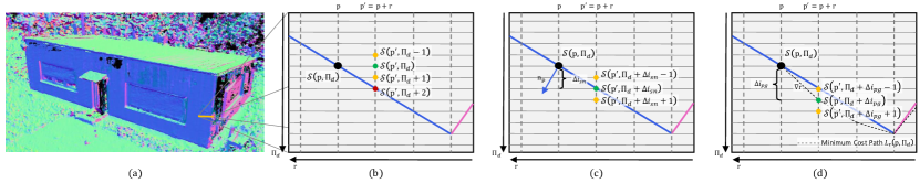
Figure 2: Illustration of the SGM^x path aggregation along one path direction $\mathrm{r}$. (a) Normal map of a building. The yellow line indicates the area for which the SGM^x path aggregation is shown. (b) Illustration of the SGM^fp path aggregation. The blue and pink lines correspond to blue and pink surface orientations on the building facade. When aggregating the path costs for pixel $\mathrm{p}$ at plane $\Pi_{d}$, SGM^fp will incorporate the previous costs at the same plane position (green) without additional penalty. The previous path costs at $\Pi_{d}\,\pm 1$ (yellow) will be penalized with $P_{1}$. The previous path costs located at $\Pi_{d}+2$ (red), which is actually located on the corresponding surface, will be penalized with the highest penalty $P_{2}$. (c) SGM^sn uses the normal vector $\mathrm{n_{p}}$, encoding the surface orientation at pixel $\mathrm{p}$, and computes a discrete index jump $\Delta i_{sn}$, which adjusts the zero cost transition, causing the previous path costs at $\Pi_{d}+2$ to not be penalized. (d) Similar to SGM^sn, SGM^pg adjusts the zero cost transition. However, the discrete index jump $\Delta i_{pg}$ is derived from the running gradient $\nabla\mathrm{r}$ of the minimum cost path. As illustrated, however, this can overcompensate the shift of the zero cost transition.

The first of the proposed SGM^x extensions, which at the same time serves as a basis to the other two extensions, is a straight-forward adaptation of the standard SGM approach to the use of a fronto-parallel multi-view plane-sweep sampling as part of the work flow presented in Figure 1. It is thus denoted as fronto-parallel SGM (SGM^fp) and was already used in (Ruf et al., , 2017) and (Ruf et al., 2018b, ). The recursive aggregation of the matching costs along each path is adjusted to

$$L_{\mathrm{r}}(\mathrm{p},\Pi_{d})= \mathcal{S}(\mathrm{p},\Pi_{d})\ +\$$ (5)

$$\min\limits_{d^{\prime}\in\mathcal{D}}\left(L_{\mathrm{r}}(\mathrm{p-r},\Pi_{d^{\prime}})+\mathcal{V}_{fp}(\Pi_{d},\Pi_{d^{\prime}})\right),$$

with $\Pi_{d}$ being the sampling plane at depth $d$ used to perform the multi-image matching. Here, instead of penalizing the deviations in neighboring disparities, the smoothness term $\mathcal{V}_{fp}$ penalizes different planes between adjacent pixels along the path $L_{\mathrm{r}}$:

$$\mathcal{V}_{fp}(\Pi_{d},\Pi_{d^{\prime}}) =\begin{cases}0&,\ \text{if}\ \Gamma(\Pi_{d})=\Gamma(\Pi_{d^{\prime}})\\ P_{1}&,\ \text{if}\ \left|\Gamma(\Pi_{d})-\Gamma(\Pi_{d^{\prime}})\right|=1\\ P_{2}&,\ \text{if}\ \left|\Gamma(\Pi_{d})-\Gamma(\Pi_{d^{\prime}})\right|>1,\end{cases}$$ (6)

with $\Gamma(\cdot)$ being a function that returns the index of $\Pi_{d}$ within the set of sampling planes (cf. Figure 2(b)).

In our second extension, namely surface normal SGM (SGM^sn), we adopt the approach presented by Scharstein et al., (2017) to use surface normals to adjust the zero-cost transition to coincide with the surface orientation. We use a normal map $N$ corresponding to $I_{\mathrm{ref}}$ that holds the surface normals of the scene that is to be reconstructed. We assume $N$ to be given or use the normal map that has been predicted in the previous iteration of our hierarchical work flow (cf. Figure 1). Assuming that a surface normal vector $\mathrm{n}_{\mathrm{p}}=N(\mathrm{p})$ corresponding to the surface orientation at pixel $\mathrm{p}$ is given, we compute the discrete index jump ${\Delta i}_{sn}$ through the set of sampling planes that is caused by the tangent plane to $\mathrm{n}_{\mathrm{p}}$ at the scene point $\mathrm{X_{p}}$, in which the ray through $\mathrm{p}$ intersects $\Pi_{d}$. As also stated by Scharstein et al., (2017), these discrete index jumps can be computed once for each pixel $\mathrm{p}$ and each path direction $\mathrm{r}$ (cf. Figure 2(c)). Given ${\Delta i}_{sn}$, we adjust the smoothness term used in SGM^sn according to

$$\mathcal{V}_{sn}(\Pi_{d},\Pi_{d^{\prime}})=\mathcal{V}_{fp}(\Pi_{d}+{\Delta i}_{sn},\Pi_{d^{\prime}}).$$ (7)

The third extension does not consider any additional information, such as surface normals $N$, while computing the aggregating path costs $L_{\mathrm{r}}(\mathrm{p},\Pi_{d})$. Instead, it relies on the gradient $\nabla\mathrm{r}$ in scene space corresponding to the minimal path costs and is therefore denoted as path gradient SGM (SGM^pg). Here, we again consider $\mathrm{X_{p}}$ as the scene point corresponding to the intersection between the ray through $\mathrm{p}$ and $\Pi_{d}$. Furthermore, we denote $\mathrm{p^{\prime}}=\mathrm{p+r}$ as predecessor of $\mathrm{p}$ along the path $\mathrm{r}$ and $\mathrm{\hat{X}_{p^{\prime}}}$ as the scene point parameterized by $\mathrm{p^{\prime}}$ and the plane $\Pi_{\hat{d}}$. The latter represents the plane at depth $\hat{d}=\operatorname*{arg\,min}_{d^{\prime}\in\mathcal{D}}{L_{\mathrm{r}}(\mathrm{p^{\prime}},\Pi_{d^{\prime}})}$ associated with the previous minimal path costs. From this, we dynamically compute a gradient vector $\nabla\mathrm{r}=\mathrm{X_{p}}-\mathrm{\hat{X}_{p^{\prime}}}$ in scene space while traversing along the path $\mathrm{r}$. Given $\nabla\mathrm{r}$, we again compute a discrete index jump ${\Delta i}_{pg}$ through the set of sampling planes and use

$$\mathcal{V}_{pg}(\Pi_{d},\Pi_{d^{\prime}})=\mathcal{V}_{fp}(\Pi_{d}+{\Delta i}_{pg},\Pi_{d^{\prime}})$$ (8)

to dynamically adjust the zero-cost transition to possibly slanted surfaces in scene space (cf. Figure 2(d)). This allows us to implicitly penalize deviations from the running gradient vector in scene space between two consecutive pixels along the path $\mathrm{r}$.

Since our extensions SGM^x only affect the path-wise aggregation of the matching costs, we extract the depth map $D$ analogously to Equation 3 and Equation 4, substituting the disparity by the depths corresponding to the set of sampling planes. Note that, since our sampling set consists of fronto-parallel planes, we can directly extract the depth from their parameterization. If slanted planes are used for sampling, a pixel-wise intersection of the viewing rays with the winning planes is to be performed in order to extract $D$.

Finally, for each of the extensions, a median filter with a kernel size of $5\times 5$ is used to further reduce noise.

3.3 Adaptive smoothness penalty

Hirschmueller, (2005, 2008) suggests to adaptively adjust the penalty $P_{2}$ to the image gradient along path $\mathrm{r}$ in order to preserve depth discontinuities at object boundaries. In this work, we evaluate two different strategies to adjust $P_{2}$. The first strategy fully relies on the absolute intensity difference ($|\Delta I|$) between consecutive pixels:

$$P_{2}^{\Delta I}=P_{1}\left(1+\alpha\exp\left(-\frac{|\Delta I|}{\beta}\right)\right)$$ (9)

with $\alpha=8$ and $\beta=10$ according to Scharstein et al., (2017).

A second strategy that has been proposed by Ruf et al., 2018b relies on the use of a line segment detector (Grompone von Gioi et al., , 2010) to generate a binary line image of the reference image $I_{\mathrm{ref}}^{line}$ and reduce $P_{2}^{line}$ to $P_{1}$ at a detected line segment:

$$P_{2}^{line} =\begin{cases}P_{1}&,\ \text{if}\ I^{line}_{\mathrm{ref}}(\mathrm{p})=1\\ P_{2}&,\ \text{otherwise}.\end{cases}$$ (10)

Ruf et al., 2018b argue that this allows to enforce strong discontinuities at object boundaries while increasing the smoothness within objects.

3.4 Confidence measure

We additionally compute a confidence map $C$, holding per-pixel confidence measures of the depth estimates in the range of $\left[0,1\right]$. For this, we model two confidence measures that solely rely on the results of the SGM path aggregation. With our first measure $U_{p}$, we adopt the observation of Drory et al., (2014), that the sum of the individual minimal path costs at pixel $\mathrm{p}$ is a lower bound of the winning aggregated costs:

$$U_{p} =\min\limits_{d}{\bar{\mathcal{S}}(\mathrm{p},\Pi_{d})}-\sum\limits_{\mathrm{r}}{\min\limits_{d}{L_{\mathrm{r}}(\mathrm{p},\Pi_{d})}}.$$ (11)

The second confidence measure $U_{u}$ models the uniqueness of the winning aggregated costs, i.e. the difference between the lowest and second-lowest aggregated costs for each pixel in $\bar{\mathcal{S}}$:

$$U_{u}= \min\limits_{d}\left(\bar{\mathcal{S}}(\mathrm{p},\Pi_{d})\backslash\min\limits_{d}{\bar{\mathcal{S}}(\mathrm{p},\Pi_{d})}\right)-$$ (12)

$$\min\limits_{d}{\bar{\mathcal{S}}(\mathrm{p},\Pi_{d})}.$$

Given the above measures, we compute the final pixel-wise confidence value according to

$$C(\mathrm{p})=\exp\left(-\frac{U_{p}}{\varphi}\right)\cdot\min\left\{\exp\left(U_{u}-\tau\right),1\right\}.$$ (13)

In this equation, the first term will resolve to 1, if $U_{p}=0$, i.e. the winning costs equal the sum of the minimal path costs. If this is not the case, the rate of the exponential decay of the confidence is controlled by the parameter $\varphi$.

The parameter $\tau$ represents the uniqueness threshold of the winning solution. If the absolute difference between the lowest and second-lowest pixel-wise aggregated costs in $\bar{\mathcal{S}}$ is above the threshold $\tau$, the second term of Equation 13 will resolve to 1.

In our evaluation, this confidence measure is used to plot the accuracy of the predicted depth maps with respect to their completeness, where the latter is computed by thresholding the corresponding confidence map (cf. Figure 3(b)).

3.5 Normal map estimation

The third output of our algorithm is a normal map $N$ that holds the surface orientation in the depth map $D$ at pixel $\mathrm{p}$. For the computation of the surface normal, we reproject the depth map into a point cloud and compute the cross product $\mathrm{n_{p}}=\mathrm{h_{p}}\times\mathrm{v_{p}}$. Here, $\mathrm{h_{p}}$ denotes a vector between the scene points of two neighboring pixels to $\mathrm{p}$ in horizontal direction, while $\mathrm{v_{p}}$ is the vector between the scene points of two vertical neighboring pixels.

Since the computation of $N$ does not contain any smoothness assumption, we apply an a-posteriori smoothing to the normal map, the so-called Gestalt-Smoothing. In particular, we perform an appearance-based weighted Gaussian smoothing in a local two-dimensional neighborhood $\mathcal{N}_{\mathrm{p}}$ around $\mathrm{p}$:

$$N(\mathrm{p})=\frac{\bar{\mathrm{n}}_{\mathrm{p}}}{\left|\bar{\mathrm{n}}_{\mathrm{p}}\right|},$$ (14)

with

$$\bar{\mathrm{n}}_{\mathrm{p}}=\mathrm{n_{p}}+\sum\limits_{\mathrm{q}\in\mathcal{N}_{\mathrm{p}}}\left[\mathrm{n_{q}}\cdot\frac{1}{\sqrt{2\pi\sigma^{2}}}\exp\left(-\frac{\left(\mathrm{q}-\mathrm{p}\right)^{2}}{2\sigma^{2}}\right)\right.$$ (15)

$$\left.\cdot\exp\left(-\frac{|I_{\mathrm{q}}-I_{\mathrm{p}}|}{\beta}\right)\right],$$

where $\beta=10$ in accordance with Equation 9, and $\sigma$ is fixed to the radius of the local smoothing neighborhood.

4 EVALUATION

4.1 Experiments

	DTU		TMB
Configuration Name	mL1-abs	mL1-rel	mL1-abs	mL1-rel
SGMfp-CT-$P_{2}^{\Delta I}$	10.362 $\pm$11.867	0.014 $\pm$0.015	0.392 $\pm$0.336	0.712 $\pm$0.486
SGMfp-CT-$P_{2}^{line}$	10.392 $\pm$12.065	0.014 $\pm$0.015	0.406 $\pm$0.358	0.713 $\pm$0.485
SGMfp-NCC-$P_{2}^{\Delta I}$	9.859 $\pm$11.781	0.014 $\pm$0.015	0.406 $\pm$0.347	0.704 $\pm$0.480
SGMfp-NCC-$P_{2}^{line}$	12.588 $\pm$13.493	0.017 $\pm$0.017	0.492 $\pm$0.435	0.704 $\pm$0.461
SGMsn-CT-$P_{2}^{\Delta I}$	10.106 $\pm$11.532	0.014 $\pm$0.015	0.401 $\pm$0.349	0.717 $\pm$0.489
SGMsn-CT-$P_{2}^{line}$	10.292 $\pm$12.068	0.014 $\pm$0.016	0.412 $\pm$0.367	0.718 $\pm$0.489
SGMsn-NCC-$P_{2}^{\Delta I}$	9.770 $\pm$11.850	0.013 $\pm$0.015	0.411 $\pm$0.351	0.705 $\pm$0.479
SGMsn-NCC-$P_{2}^{line}$	12.402 $\pm$13.405	0.017 $\pm$0.017	0.491 $\pm$0.434	0.704 $\pm$0.460
SGMpg-CT-$P_{2}^{\Delta I}$	10.612 $\pm$11.919	0.015 $\pm$0.015	0.401 $\pm$0.339	0.718 $\pm$0.493
SGMpg-CT-$P_{2}^{line}$	10.529 $\pm$12.014	0.015 $\pm$0.015	0.413 $\pm$0.359	0.712 $\pm$0.492
SGMpg-NCC-$P_{2}^{\Delta I}$	10.010 $\pm$11.739	0.014 $\pm$0.015	0.417 $\pm$0.344	0.710 $\pm$0.481
SGMpg-NCC-$P_{2}^{line}$	12.598 $\pm$13.358	0.017 $\pm$0.017	0.495 $\pm$0.432	0.706 $\pm$0.461
COLMAP	3.309 $\pm$4.156	0.005 $\pm$0.006	-	-

(a) Quantitative results of all twelve configurations which are evaluated on the DTU and TMB dataset. For each dataset, the mean absolute L1 error (mL1-abs) as well as the mean relative L1 error (mL1-rel) are evaluated. The configuration name encodes the different configuration settings. Here, the first part represents the extension used, the middle section holds the cost function which was applied in the multi-image matching, and the third portion represents the strategy, which was adopted to adapt the $P_{2}$ penalty. The last row denotes the results achieved by the offline SfM pipeline COLMAP (Schönberger et al., , 2016; Schönberger and Frahm, , 2016).

(b) ROC curves plotting normalized mean L1-rel over the confidence threshold which is used to mask the depth map. The top graph depicts the results achieved by three SGM^x configurations on the DTU dataset. The bottom graph shows the results achieved on the TMB dataset.

Figure 3: Quantitative evaluation of twelve different SGM^x configurations.

We have evaluated our approach on two different datasets, namely the DTU Robot Multi-View Stereo (MVS) dataset (Jensen et al., , 2014) and a private dataset, which is henceforth referred to as the TMB dataset.

From the DTU dataset, we have selected 21 scans of the different building models, in which each model was captured from 49 locations and with eight different lighting conditions. For our evaluation, we have used the already undistorted images with a resolution of 1600$\times$1200 pixels, captured under the most diffuse lighting. As ground truth to our approach, we have extracted depth maps from the structured light scans, which are included in the dataset, given the camera poses of the reference image.

Our privately captured TMB dataset consists of three different scenes captured with a DJI Phantom 3 Professional from multiple different aerial viewpoints. The images were captured while flying around the objects of interest at three different altitudes (8 m, 10 m and 15 m). Each image was resized to 1920$\times$1080 pixels before used for our evaluation. We compare the results achieved by the proposed approach to data from an offline SfM pipeline for accurate and dense 3D image matching. For this, we have used COLMAP (Schönberger et al., , 2016; Schönberger and Frahm, , 2016) to reconstruct the considered scenes of the dataset. As a required input to our algorithm, we have used the camera poses computed by the sparse reconstruction. In the evaluation, we have compared the depth maps predicted by our algorithm against the geometric depth maps from the dense reconstruction of COLMAP.

As an accuracy measure between the estimates and the ground truth, we have used an absolute and relative L1 measure, which is computed pixel-wise and averaged over the number of estimates in the depth map:

$$\text{L1-abs}(d,\hat{d})=\frac{1}{m}\sum\limits_{i}{|d_{i}-\hat{d}_{i}|},$$ (16)

$$\text{L1-rel}(d,\hat{d})=\frac{1}{m}\sum\limits_{i}{\frac{|d_{i}-\hat{d}_{i}|}{\hat{d}_{i}}},$$ (17)

with $d$ and $\hat{d}$ denoting the predicted and ground truth depth values respectively, and with $m$ being the number of pixels for which both $d$ and $\hat{d}$ exists. Here, the depth values denote the fronto-parallel distances of the corresponding scene points from the image center of the reference camera. Both measures are only evaluated for pixels which contain a predicted and ground truth depth value. While L1-abs denotes the average absolute difference between the prediction and the ground truth, L1-rel computes the depth error relative to the ground truth depth. This reduces the influence of a high absolute error where the ground truth depth is large and increases the influence of measurements close to the camera. This is important, as the uncertainty of the depth measurements typically increases with the distance from the camera.

The parameterization of our algorithms was determined empirically based on the results, which were achieved on the DTU dataset. For our hierarchical processing scheme, we have used $L=3$ pyramid levels and have set $\Delta d=6$ for the computation of the per-pixel sampling range, yielding the best trade-off between accuracy and runtime. The support region of the normalized cross correlation (NCC) and the Census Transform (CT) was set to 5$\times$5 and 9$\times$7, respectively, where the latter is the maximum size for which the CT bit string still fits into a 64 bit integer. In the computation of the normal map, we have used a smoothing kernel of size 21$\times$21 for the Gestalt-Smoothing.

Due to the different range of values in the cost functions, the parameterization of the penalty functions and the confidence measures need to be chosen accordingly. For the NCC similarity measure, we have set $P_{1}=150$ when using $P_{2}^{\Delta I}$ and $P_{1}=60,P_{2}=220$ when using $P_{2}^{line}$. In case of the CT, we have set $P_{1}=15$ when using $P_{2}^{\Delta I}$ and $P_{1}=10,P_{2}=55$ when using $P_{2}^{line}$. For the computation of the confidence measure (cf. Equation 13), we have set $\varphi=80,\tau=10$ when using the NCC, and $\varphi=650,\tau=80$ when using the CT.

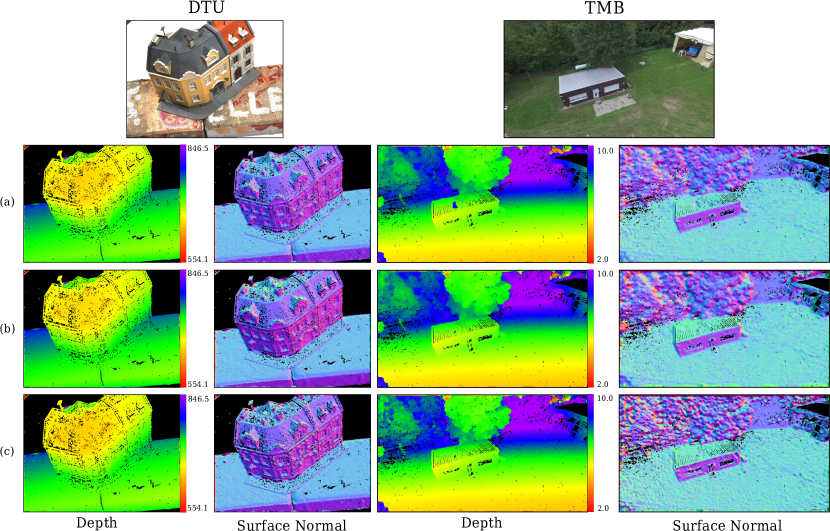
Figure 4: Qualitative comparison between the results achieved by the SGM^fp-NCC-$P_{2}^{\Delta I}$ (Row (a)), SGM^sn-NCC-$P_{2}^{\Delta I}$ (Row (b)) and SGM^pg-NCC-$P_{2}^{\Delta I}$ (Row (c)). Note that the depth and normal maps are filtered by the DoG filter and according to the available data in the ground truth.

All experiments were performed on a desktop hardware with an Intel Core i7-5820K CPU 3.3GHz and a NVIDIA GeForce GTX 1070 GPU. The computationally expensive part of our algorithm, such as depth and normal map estimation, is optimized with CUDA to run on the GPU, achieving a frame rate of 1Hz$-$2Hz for full HD imagery, depending on the configuration and parameterization used.

In the scope of this work, we have evaluated twelve different configurations of our SGM^x extensions. The results achieved by these configurations on the two datasets are listed in Figure 3(a). The configuration names denote the corresponding setups. In comparison, the results achieved by the offline SfM pipeline COLMAP are listed in the last row of Figure 3(a). The values in the depth maps are in the range of $\left[554.1,846.5\right]$ in case of the DTU dataset, and $\left[2.0,10\right]$ in the depth maps corresponding to the TMB dataset (cf. Figure 4). Since the datasets do not have any metric system, the errors are without any unit. However, the given ranges of values in the depth maps allow to draw conclusions on these error values with respect to the estimates.

For each of the three SGM^x extensions, we have chosen one configuration, namely the one with the lowest average error (underlined values), and plotted ROC curves for both datasets (cf. Figure 3(b)). These curves represent the mean relative L1 error, normalized by the density, over the confidence threshold, which is used to mask the corresponding depth map. A qualitative comparison between the three different SGM^x extensions is done on one example image from each of the two datasets (cf. Figure 4). Here, the depth and normal maps are filtered by the DoG filter and according to available data in the ground truth. A discussion of the experimental results is given in the section below.

4.2 Discussion of the experimental results

The experimental results listed in Figure 3 reveal a number of strengths and weaknesses of the proposed SGM^x extensions. Starting off with the strengths, the numbers in Figure 3(a) show similar accuracies between all three extensions. Especially when considering the value ranges in the depth maps one can argue that, with an absolute error of 1%$-$4% of the maximum depth range, all SGM^x approaches achieve a high accuracy with respect to the ground truth. The differences in accuracy between the two datasets can be attributed to the fact that the parameters of our approach were fine-tuned with respect to the DTU dataset. Furthermore, since the ranges of depth values in the TMB dataset are much smaller than the ones in the DTU dataset, a minor difference between the estimate and the ground truth has a greater influence on the resulting error, which opposes the implication of a possible parametric over-fitting with respect to the DTU dataset.

A comparison between the three SGM^x extensions, solely based on the values listed in Figure 3(a), does not allow to conclude that the consideration of surface normals significantly increases the accuracy of the resulting depth map. In fact, looking at the results from the TMB dataset, the mean errors achieved by SGM^fp are lower than the ones achieved by SGM^sn and SGM^pg. However, the ROC curves in Figure 3(b) reveal that the use of surface normals increases the ratio between the accuracy of the measurements and their confidence. This assumption is also encouraged by a qualitative comparison based on the results depicted in Figure 4. The use of surface normals yields a slightly more consistent normal map, in particular when comparing the roof of the buildings. This supports the claims of Scharstein et al., (2017).

However, the qualitative comparison also reveals that the depth discontinuities at object boundaries are less concise when considering surface normals in the SGM optimization. While this could result from the adjustment of the zero transition in the path aggregation, it cannot be ruled out that this is due to less appropriate parameterization of the penalty functions. Furthermore, the evaluation reveals that the results achieved by SGM^pg are inferior to the ones of SGM^fp and SGM^sn as the normal maps are more noisy compared to the other results. While a cause of this effect could not be fully resolved in the scope of this work, we believe that this might be attributed to an overcompensation in the extraction of the zero transition shift from the gradient of the minimal cost path.

An evaluation of the different cost functions and different penalty configurations used has not revealed a clear winner. In fact, it depends on the nature of the dataset and the parameterization of the algorithm. Nonetheless, the values in Figure 3(a) suggest that, in most cases, the use of NCC in the image matching and $P_{2}^{\Delta I}$ in the SGM optimization is an appropriate choice.

Lastly, in this work, we have only considered the use of fronto-parallel plane orientation while performing the plane-sweep multi-image matching. Yet, Gallup et al., (2007) and Sinha et al., (2014) suggest to use multiple sweeping directions for the plane-sweep sampling. Doing so would not require to incorporate surface orientations in the SGM optimization, but allow to use the standard SGM (cf. SGM^fp) in its adaption to plane-sweep stereo as done by Sinha et al., (2014). An evaluation of this is an interesting direction for future work.

5 CONCLUSION & FUTURE WORK

In conclusion, this work proposes a hierarchical algorithm for efficient depth and normal map estimation from oblique aerial imagery based on plane-sweep multi-image matching followed by a semi-global matching optimization for cost aggregation and regularization. Our approach allows to additionally consider local surface orientations in the computation of the depth map.

Both the standard SGM optimization and the adjustment of the same with respect to local surface normals, achieve results with high accuracies. However, our experiments support the claims of Scharstein et al., (2017) that the consideration of surface normals achieves more consistent results with higher confidence in homogeneous areas. Furthermore, the quantitative evaluation reveals that our results are comparable to the ones achieved by sophisticated SfM pipelines such as COLMAP. In contrast, however, our approach only considers a confined image bundle of an input sequence allowing to perform an online computation at 1Hz$-$2Hz.

Nonetheless, the experimental results have also revealed a number of improvements and considerations that are promising options for future work. An example is the mentioned incorporation of multiple plane orientations in the process of plane-sweep multi-image matching. Another aspect, which is to be considered in future work, is the computation and evaluation of the normal map. We have extracted the normal map solely based on the geometric information in the depth map with an a-posteriori smoothing. However, the use of a more sophisticated method would greatly improve the results.

REFERENCES

- Banz et al., (2011) Banz, C., Blume, H. and Pirsch, P., 2011. Real-time semi-global matching disparity estimation on the GPU. In: Proc. IEEE Int. Conf. on Computer Vision Workshops, pp. 514–521.
- Barry et al., (2015) Barry, A. J., Oleynikova, H., Honegger, D., Pollefeys, M. and Tedrake, R., 2015. FPGA vs pushbroom stereo vision for UAVs. In: Proc. IROS Workshop on Vision-based Control and Navigation of Small Lightweight UAVs.
- Blaha et al., (2016) Blaha, M., Vogel, C., Richard, A., Wegner, J. D., Pock, T. and Schindler, K., 2016. Large-scale semantic 3d reconstruction: an adaptive multi-resolution model for multi-class volumetric labeling. In: Proc. IEEE Conf. on Computer Vision and Pattern Recognition, pp. 3176–3184.
- Bulatov et al., (2011) Bulatov, D., Wernerus, P. and Heipke, C., 2011. Multi-view dense matching supported by triangular meshes. ISPRS Journal of Photogrammetry and Remote Sensing 66(6), pp. 907–918.
- Collins, (1996) Collins, R. T., 1996. A space-sweep approach to true multi-image matching. In: Proc. IEEE Conf. on Computer Vision and Pattern Recognition, pp. 358–363.
- Drory et al., (2014) Drory, A., Haubold, C., Avidan, S. and Hamprecht, F. A., 2014. Semi-global matching: a principled derivation in terms of message passing. In: Proc. German Conf. on Pattern Recognition, pp. 43–53.
- Gallup et al., (2007) Gallup, D., Frahm, J.-M., Mordohai, P., Yang, Q. and Pollefeys, M., 2007. Real-time plane-sweeping stereo with multiple sweeping directions. In: Proc. IEEE Conf. on Computer Vision and Pattern Recognition, pp. 1–8.
- Gehrig and Rabe, (2010) Gehrig, S. K. and Rabe, C., 2010. Real-time semi-global matching on the CPU. In: Proc. IEEE Conf. on Computer Vision and Pattern Recognition Workshops, pp. 85–92.
- Grompone von Gioi et al., (2010) Grompone von Gioi, R., Jakubowicz, J., Morel, J.-M. and Randall, G., 2010. LSD: A fast line segment detector with a false detection control. IEEE Transactions on Pattern Analysis and Machine Intelligence 32(4), pp. 722–732.
- Hermann et al., (2009) Hermann, S., Klette, R. and Destefanis, E., 2009. Inclusion of a second-order prior into semi-global matching. In: Proc. Pacific-Rim Symposium on Image and Video Technology, pp. 633–644.
- Hirschmueller, (2005) Hirschmueller, H., 2005. Accurate and efficient stereo processing by semi-global matching and mutual information. In: Proc. IEEE Conf. on Computer Vision and Pattern Recognition, Vol. 2, pp. 807–814.
- Hirschmueller, (2008) Hirschmueller, H., 2008. Stereo processing by semiglobal matching and mutual information. IEEE Transactions on Pattern Analysis and Machine Intelligence 30(2), pp. 328–341.
- Hofmann et al., (2016) Hofmann, J., Korinth, J. and Koch, A., 2016. A scalable high-performance hardware architecture for real-time stereo vision by semi-global matching. In: Proc. IEEE Conf. on Computer Vision and Pattern Recognition Workshops, pp. 27–35.
- Jensen et al., (2014) Jensen, R., Dahl, A., Vogiatzis, G., Tola, E. and Aanæs, H., 2014. Large scale multi-view stereopsis evaluation. In: Proc. IEEE Conf. on Computer Vision and Pattern Recognition, pp. 406–413.
- Kang et al., (2001) Kang, S. B., Szeliski, R. and Chai, J., 2001. Handling occlusions in dense multi-view stereo. In: Proc. IEEE Conf. on Computer Vision and Pattern Recognition, Vol. 1, pp. 103–110.
- Menze and Geiger, (2015) Menze, M. and Geiger, A., 2015. Object scene flow for autonomous vehicles. In: Proc. IEEE Conf. on Computer Vision and Pattern Recognition, pp. 3061–3070.
- Musialski et al., (2013) Musialski, P., Wonka, P., Aliaga, D. G., Wimmer, M., van Gool, L. and Purgathofer, W., 2013. A survey of urban reconstruction. Computer Graphics Forum 32(6), pp. 146–177.
- Ni et al., (2018) Ni, J., Li, Q., Liu, Y. and Zhou, Y., 2018. Second-order semi-global stereo matching algorithm based on slanted plane iterative optimization. IEEE Access 6, pp. 61735–61747.
- Rothermel et al., (2014) Rothermel, M., Haala, N., Wenzel, K. and Bulatov, D., 2014. Fast and robust generation of semantic urban terrain models from UAV video streams. In: Proc. Int. Conf. on Pattern Recognition, pp. 592–597.
- Rothermel et al., (2012) Rothermel, M., Wenzel, K., Fritsch, D. and Haala, N., 2012. SURE: Photogrammetric surface reconstruction from imagery. In: Proc. LowCost3D Workshop, Berlin, Germany, Vol. 8.
- Ruf et al., (2017) Ruf, B., Erdnuess, B. and Weinmann, M., 2017. Determining plane-sweep sampling points in image space using the cross-ratio for image-based depth estimation. Int. Archives of the Photogrammetry, Remote Sensing and Spatial Information Sciences XLII-2/W6, pp. 325–332.
- (22) Ruf, B., Monka, S., Kollmann, M. and Grinberg, M., 2018a. Real-time on-board obstacle avoidance for UAVs based on embedded stereo vision. Int. Archives of the Photogrammetry, Remote Sensing and Spatial Information Sciences XLII-1, pp. 363–370.
- (23) Ruf, B., Thiel, L. and Weinmann, M., 2018b. Deep cross-domain building extraction for selective depth estimation from oblique aerial imagery. ISPRS Annals of Photogrammetry, Remote Sensing and Spatial Information Sciences IV-1, pp. 125–132.
- Scaramuzza et al., (2014) Scaramuzza, D., Achtelik, M. C., Doitsidis, L., Friedrich, F., Kosmatopoulos, E., Martinelli, A., Achtelik, M. W., Chli, M., Chatzichristofis, S., Kneip, L. et al., 2014. Vision-controlled micro flying robots: from system design to autonomous navigation and mapping in GPS-denied environments. IEEE Robotics & Automation Magazine 21(3), pp. 26–40.
- Scharstein and Szeliski, (2002) Scharstein, D. and Szeliski, R., 2002. A taxonomy and evaluation of dense two-frame stereo correspondence algorithms. Int. Journal of Computer Vision 47(1-3), pp. 7–42.
- Scharstein et al., (2017) Scharstein, D., Taniai, T. and Sinha, S. N., 2017. Semi-global stereo matching with surface orientation priors. In: Proc. Int. Conf. on 3D Vision, pp. 215–224.
- Schönberger and Frahm, (2016) Schönberger, J. L. and Frahm, J.-M., 2016. Structure-from-motion revisited. In: Proc. IEEE Conf. on Computer Vision and Pattern Recognition, pp. 4104–4113.
- Schönberger et al., (2016) Schönberger, J. L., Zheng, E., Frahm, J.-M. and Pollefeys, M., 2016. Pixelwise view selection for unstructured multi-view stereo. In: Proc. Europ. Conf. on Computer Vision, pp. 501–518.
- Sinha et al., (2014) Sinha, S. N., Scharstein, D. and Szeliski, R., 2014. Efficient high-resolution stereo matching using local plane sweeps. In: Proc. IEEE Conf. on Computer Vision and Pattern Recognition, pp. 1582–1589.
- Spangenberg et al., (2014) Spangenberg, R., Langner, T., Adfeldt, S. and Rojas, R., 2014. Large scale semi-global matching on the CPU. In: Proc. IEEE Intelligent Vehicles Symposium, pp. 195–201.
- Taneja et al., (2015) Taneja, A., Ballan, L. and Pollefeys, M., 2015. Geometric change detection in urban environments using images. IEEE Transactions on Pattern Analysis and Machine Intelligence 37(11), pp. 2193–2206.
- Weinmann, (2016) Weinmann, M., 2016. Reconstruction and analysis of 3D scenes – From irregularly distributed 3D points to object classes. Springer, Cham, Switzerland.
- Wenzel, (2016) Wenzel, K., 2016. Dense image matching for close range photogrammetry. PhD thesis, University of Stuttgart, Germany.
- Wenzel et al., (2013) Wenzel, K., Rothermel, M., Haala, N. and Fritsch, D., 2013. SURE – the IFP software for dense image matching. In: Proc. Photogrammetric Week, pp. 59–70.
- Zabih and Woodfill, (1994) Zabih, R. and Woodfill, J., 1994. Non-parametric local transforms for computing visual correspondence. In: Proc. Europ. Conf. on Computer Vision, pp. 151–158.