Construction of wavelet dictionaries for ECG modelling

Abstract

Background and Objective: The purpose of sparse modelling of ECG signals is to represent an ECG record, given by sample points, as a linear combination of as few elementary components as possible. This can be achieved by creating a redundant set, called a dictionary, from where the elementary components are selected. The success in sparsely representing an ECG record depends on the nature of the dictionary being considered. In this paper we focus on the construction of different families of wavelet dictionaries, which are appropriate for the purpose of reducing dimensionality of ECG signals through sparse representation modelling.

Method: The suitability of wavelet dictionaries for ECG modelling, applying the Optimized Orthogonal Matching Pursuit approach for the selection process, was demonstrated in a previous work on the MIT-BIH Arrhythmia database consisting of 48 records each of which of 30 min length. This paper complements the previous one by presenting the technical details, methods, algorithms, and MATLAB software facilitating the construction of different families of wavelet dictionaries. The implementation allows for straightforward further extensions to include additional wavelet families.

Results: The sparsity in the representation of an ECG record significantly improves in relation to the sparsity produced by the corresponding wavelet basis. This result holds true for the 17 wavelet families considered here.

Conclusions: Wavelet dictionaries contribute to the representation of an ECG record as a superposition of fewer components than those needed by the wavelet basis. The software for the construction of wavelet dictionaries, which has been made available to support the material in this paper, could be of assistance to a broad range of application relying on dimensionality reduction as a first step of further ECG signal analysis.

1 Introduction

The electrocardiogram (ECG) is a routine test for clinical medicine. It plays a crucial role in the diagnosis of a broad range of anomalies in the human heart; from arrythmias to myocardial infarction.

The widely available digital ECG data has facilitated the development of algorithms for ECG processing and interpretation. In particular, the literature for computerized arrhythmia detection and classification is extensive. Useful review matterial [23, 24] can help with the introduction to state of the art techniques, which nonetheless keeps growing [1, 5, 7, 22, 29].

A common first step in ECG modeling consists in reducing the dimensionality of the signal. This entails to represent the informational content of the record by means of significantly fewer parameters than the number of samples in the digital ECG. When the aim is to reproduce the original signal at low level distortion, the step is frequently realized through transformations such as the Wavelet Transform and the Discrete Cosine Transform. In the last few years alternative approaches, falling within the category of sparse representation of ECG signals, have been considered.

Within the sparse representation framework, an ECG record is represented as a linear combination of elementary components, called atoms, which are selected from a redundant set, called a dictionary. The success of the methods developed within this framework depends on both, the selection technique and the proposed dictionary. The selection techniques which are widely applied for sparse representation of general signals are either greedy pursuit strategies [26, 30, 33], or strategies based on minimization of the 1-norm as a cost function [10]. Suitable dictionaries depend on the class of signals being processed. These can be designed at hoc or be learned from training data. Sparse representation of ECG signals has been tackled by both these approaches, e.g. [2] learns dictionaries using some part of the records for ECG compression and [31] uses Gabor dictionaries for structuring features for classification.

In a recent publication [32] we have shown that wavelet dictionaries, derived from known wavelet families, are suitable for representing an ECG record as a linear combination of fewer elementary components than those required by a wavelet basis. The model was shown to be successful for dimensionality reduction and lossy compression. As far as compression is concerned the method advanced in [32] produces compression results improving upon previously reported benchmarks [21, 25, 28, 37] for the MIT-BIH Arrhythmia data set without pre-processing. With regard to dimensionality reduction, wavelet dictionaries considerably improve upon the results achieved with the wavelet basis of the same family [32, 35]. This result motivated the present Communication. While in [32] the dictionaries have been used to demonstrate their suitability for dimensionality reduction of ECG signals at low level distortion, the details of their numerical construction were not given. This paper complements the previous work by presenting the algorithms for building dictionaries from the following mother wavelet prototypes:

1. Chui-Wang linear spline wavelet [11]

2. Chui-Wang quadratic spline wavelet [11]

3. Chui-Wang cubic spline wavelet [11]

4. primal CDF97 wavelet [6]

5. dual CDF97 wavelet [6]

6. primal CDF53 wavelet [6]

7. linear spline wavelet with short support and 2 vanishing moments [9, 20]

8. quadratic spline wavelet with short support and 3 vanishing moments [9, 20]

9. cubic spline wavelet with short support and 4 vanishing moments [9, 20]

10. Daubechies wavelet with $3$ vanishing moments [16]

11. Daubechies wavelet with $4$ vanishing moments [16]

12. Daubechies wavelet with $5$ vanishing moments [16]

13. symlet with $3$ vanishing moments [17]

14. symlet with $4$ vanishing moments [17]

15. symlet with $5$ vanishing moments [17]

16. coiflet with 2 vanishing moments and support of length 6 which is the most regular [17]

17. coiflet with 3 vanishing moments and support of length 8 [17]

The method proposed in [32] for modelling a given ECG signal proceeds as follows. Assuming that the signal is given as an $N$-dimensional array, this array is partitioned into $Q$ cells $\mathbf{f}^{\rm{c}}\{q\},q=1,\ldots,Q$. Thus, each cell $\mathbf{f}^{\rm{c}}\{q\}$ is an $N_{b}$-dimensional vector, which is modeled by an atomic decomposition of the form

$$\mathbf{f}^{\rm{a}}\{q\}=\sum_{n=1}^{k(q)}\mathbf{c}\{q\}(n)\mathbf{d}_{\ell\{q\}(n)}.$$ (1)

For each cell $q$, the atoms $\mathbf{d}_{\ell_{\{q\}(n)}},\,n=1,\ldots,k(q)$ are selected from a dictionary through the greedy Optimized Orthogonal Matching Pursuit (OOMP) algorithm [33, 34]. The array $\boldsymbol{\ell}\{q\}$ is a vector whose components $\ell\{q\}(n),\,n=1,\ldots,k(q)$ contain the indices of the selected atoms for decomposing the $q$-th cell in the signal partition. The OOMP method, for selecting these indices and computing the corresponding coefficients $\mathbf{c}\{q\},\,n=1,\ldots,k(q)$ in (1), is fully implemented by the OOMP function included as a tool of the software.

Each of the proposed dictionaries consists of two components. One of the components contains a few elements, say $M_{c}$, from a discrete cosine basis. This component of the dictionary allows for the fact that ECG signals are normally superimposed to a smooth background. It is given as a $N_{b}\times M_{c}$ matrix $\mathbf{D}^{C}$. The other component is the wavelet-based dictionary, which is given as a $N_{b}\times M_{w}$ matrix $\mathbf{D}^{W}$. Thus, the whole dictionary $\mathbf{D}$ is an $N_{b}\times(M_{c}+M_{w})$ matrix obtained by the horizontal concatenation of $\mathbf{D}^{C}$ and $\mathbf{D}^{W}$. The next section is dedicated to the construction of $\mathbf{D}^{W}$.

The paper is organized as follows. Sec. 2 gives all the details for the construction of different wavelet prototypes and the concomitant wavelet dictionaries generated by those prototypes. Secs 3 and 4 deliver details and examples demonstrating the use of the MATLAB software for modelling ECG signals within the proposed framework.

The software has been made available on a dedicated webpage [15]. The implementation allows for straightforward further extension of the options for wavelet types.

2 Method

In this section we produce all the pseudo-codes for the construction of wavelets dictionaries, which can be used to achieve the model of every segment in a signal partition. As already mentioned, each dictionary is obtained by taking the prototypes from a wavelet basis and translating them within a shorter step than that corresponding to the wavelet basis.

Throughout the paper we adopt the following notation. Boldface fonts are used to indicate Euclidean vectors and matrices. Standard mathematical fonts are used to indicate components, e.g., $\mathbf{d}\in\mathbb{R}^{N}$ is a vector of $N$-components $d(i)\in\mathbb{R},\,i=1,\ldots,N$ and $\mathbf{D}\in\mathbb{R}^{N\times M}$ is a matrix of elements $D(i,j),\,i=1\ldots,N,j=1,\ldots,M$. The symbol $L^{2}(\mathbb{R})$ denotes the space of square integrable functions.

Wavelets are usually constructed starting from a multiresolution analysis, which is a sequence $\left\{V_{j}\right\}_{j=j_{0}}^{\infty}$ of closed subspaces of the space $L^{2}\left(\mathbb{R}\right)$ which are nested and their union is dense in $L^{2}\left(\mathbb{R}\right)$, i.e.,

$$V_{j}\subset V_{j+1}\quad\forall\,j\geq j_{0},\quad\overline{\bigcup_{j=j_{0}}^{\infty}V_{j}}=L^{2}\left(\mathbb{R}\right).$$ (2)

We assume that there exists a function $\phi\in L^{2}\left(\mathbb{R}\right)$ such that for $j\geq j_{0}$ functions

$$\phi_{j,k}\left(x\right)=2^{j/2}\phi\left(2^{j}x-k\right),\quad k\in\mathbb{Z},$$ (3)

form uniformly stable bases of the spaces $V_{j}$, i.e., the bases are Riesz bases with bounds independent of the level $j$, see e.g. [8]. The functions $\phi_{j,k}$ are called scaling functions and the function $\phi$ is called a generator of scaling functions. Next we present a method for the actual construction of the scaling functions.

2.1 Generation of scaling functions

We assume that $\phi$ has a compact support $\left[0,K\right]$ for some $K\in\mathbb{N}$. From the nestedness of the multiresolution spaces $V_{j}$, it follows that there exists a scaling filter $\mathbf{h}=\left(h(1),\ldots,h(K+1)\right)$ such that

$$\phi\left(x\right)=\sum_{k=1}^{K+1}h\left(k\right)\phi\left(2x+1-k\right)\quad\forall\ x\in\mathbb{R}.$$ (4)

If $\int_{0}^{K}\phi\left(x\right)dx=c\neq 0$ then, integrating (4), we obtain

$$c=\sum_{k=1}^{K+1}h\left(k\right)\frac{c}{2}$$ (5)

which implies that $\mathbf{h}$ has to be normalized such that

$$\sum_{k=1}^{K+1}h\left(k\right)=2.$$ (6)

The scaling equation (4) enables computing values of the scaling function $\phi$ at points $k/2^{u}$ for $k=0,\ldots,K2^{u}$, $u\in\mathbb{N}$. First we compute values of $\phi$ at integer points. Since $\text{supp}\,\phi=\left[0,K\right]$, we have $\phi\left(k\right)=0$ for $k\neq\left(0,K\right)$. Let us define a vector

$$\Phi=\left(\phi\left(0\right),\ldots,\phi\left(K-1\right)\right)^{T},$$ (7)

where the $(.)^{T}$ indicates the transpose operation. Substituting $x=0,\ldots,K-1,$ into (4), we obtain

$$\Phi\left(i\right) = \phi\left(i-1\right)=\sum_{k=1}^{K+1}h\left(k\right)\phi\left(2i-1-k\right)$$

$$= \sum_{j=2i-1}^{2i-K-1}h\left(2i-j\right)\phi\left(j-1\right)=\sum_{j=2i-1}^{2i-K-1}h\left(2i-j\right)\Phi\left(j\right).$$

We set $h(k)=0$ for $k<1$ and $k>K+1$ and define a matrix $\mathbf{A}$ by

$$A\left(i,j\right)=h\left(2i-j\right),\quad i,j=1,\ldots,K.$$ (9)

Then, (2.1) is equivalent to

$$\Phi=\mathbf{A}\Phi.$$ (10)

This means that $\Phi$ is an eigenvector corresponding to the eigenvalue $1$ of the matrix $\mathbf{A}$. If the multiplicity of this eigenvalue is $1$, then $\Phi$ is given uniquely up to a multiplication by a constant. Our aim is to compute a vector $\mathbf{phi}$ such that

$$\text{phi}\left(m\right)=\phi\left(\frac{m-1}{2^{u}}\right),\quad m=1,\ldots,K\,2^{u}+1,$$ (11)

for a chosen level $u\in\mathbb{N}$. From (7) and (11) we have

$$\text{phi}\left(2^{u}\left(l-1\right)+1\right)=\phi\left(l-1\right)=\Phi\left(l\right),\quad l=1,\ldots,K.$$ (12)

We compute values of $\phi$ at points $l/2$. Note that for $l$ even we already know these values. Using (4) and (12) we obtain

$$\text{phi}\left(l2^{u-1}+1\right) = \phi\left(\frac{l}{2}\right)=\sum_{k=1}^{K+1}h\left(k\right)\phi\left(l+1-k\right)$$

$$= \sum_{k=1}^{K+1}h\left(k\right)\text{phi}\left(\left(l+1-k\right)2^{u}+1\right)$$

for $l=1,3,\ldots,2N-1$. Similarly, we compute values of $\phi$ at points $l/4$, and thus we continue until we determine values at points $l/2^{u}$. More precisely, for $i=1,\ldots,u$ we assume that we know values of $\phi$ at $l/2^{i-1}$, $l=0,\ldots,K2^{i-1}+1,$ and we compute the values

$$\text{phi}\left(m\right)=\phi\left(x\right),\quad m=x2^{u}+1,\quad x=l/2^{i-1}+1/2^{i}.$$ (14)

Using (4) we obtain

$$\text{phi}\left(m\right) = \phi\left(x\right)=\sum_{k=1}^{K+1}h\left(k\right)\phi\left(2x+1-k\right)$$

$$= \sum_{k=1}^{K+1}h\left(k\right)\text{phi}\left(\left(2x+1-k\right)2^{u}+1\right).$$

Remark 1.

Some scaling functions such as spline scaling functions are known in an explicit form and their values can be evaluated directly. However, an advantage of our approach is that it is more general and can be used for a large class of wavelet families.

2.2 Construction of wavelet generators from scaling functions

Let $W_{j}$ be complement spaces such that $V_{j+1}=V_{j}\oplus W_{j}$, where $\oplus$ denotes a direct sum. Wavelet functions $\psi_{j,k}$ are constructed in the form:

$$\psi_{j,k}\left(x\right)=2^{j/2}\psi\left(2^{j}x-k\right),\quad k\in\mathbb{Z},$$ (16)

to be a basis for $W_{j}$ and such that

$$\mathcal{B}=\left\{\phi_{j_{0},k},k\in\mathbb{Z}\right\}\cup\left\{\psi_{j,k},k\in\mathbb{Z},j\geq j_{0}\right\}$$ (17)

called a wavelet basis, is a Riesz basis of the space $L^{2}\left(\mathbb{R}\right)$.

Since $W_{j}\subset V_{j+1}$ there exists a vector $\mathbf{g}=\left(g(1),\ldots,g(M+1)\right)$ such that

$$\psi\left(x\right)=\sum_{k=1}^{M+1}g\left(k\right)\phi\left(2x+1-k\right).$$ (18)

The vector $\mathbf{g}$ is called a wavelet filter. From (18) we have

$$\text{supp}\,\psi=\left[0,\frac{M+K}{2}\right].$$ (19)

In Algorithm 1 we compute a vector $\mathbf{psi}$ such that

$$\text{psi}\left(m\right)=\psi\left(\frac{m-1}{2^{u}}\right),\quad m=1,\ldots,\left(M+K\right)2^{u-1}+1,$$ (20)

in the following way. Due to (18) and (20), we have

$$\text{psi}\left(m\right) = \psi\left(\frac{m-1}{2^{u}}\right)=\sum_{k=1}^{M+1}g\left(k\right)\phi\left(\left(m-1\right)\,2^{1-u}+1-k\right)$$ (21)

$$= \sum_{k=1}^{M+1}g\left(k\right)\text{phi}\left(2m-1+\left(1-k\right)\,2^{u}\right).$$

The sum in the last equation is computed as a cyclic sum. For

$$m=1,\ldots,(M+K)2^{u-1}+1$$ (22)

we set $\text{psi}\left(m\right)=0$ and for $k=1,\ldots,M+1$ we do

$$\text{psi}\left(m\right)=\text{psi}\left(m\right)+g\left(k\right)\text{phi}\left(2m-1+\left(1-k\right)\,2^{u}\right),$$ (23)

if $1\leq 2m-1+\left(1-k\right)\,2^{u}\leq K2^{u}+1$. Using the substitution

$$2m-1+\left(1-k\right)\,2^{u}\ =2i-1,$$ (24)

for $i=1,\ldots,K2^{u-1}+1$, we obtain

$$\text{psi}\left(i+\left(k-1\right)2^{u-1}\right)=\text{psi}\left(i+\left(k-1\right)2^{u-1}\right)+g\left(k\right)\text{phi}\left(2i-1\right).$$ (25)

Algorithm 1 computes vectors $\mathbf{phi}$ and $\mathbf{psi}$ for given scaling and wavelet filters. The filters corresponding to the wavelet families supported by the software are given in Appendix A (Algorithm 8).

Algorithm 1
Procedure [$\mathbf{phi}$,$\mathbf{psi}$] = WaveletGen($\mathbf{h}$,$\mathbf{g}$,u)

   Input:  

$\mathbf{h}$	scaling filter
$\mathbf{g}$	wavelet filter
$u$	level (integer) that determines points $l/2^{u}$

   Output: 

$\mathbf{phi}$	vector of scaling function values (c.f. (11))
$\mathbf{psi}$	vector of wavelet values (c.f. (20))

   $K=\text{length}(\mathbf{h})-1$ {support length of $\phi$}

   $\mathbf{h}=2\,\mathbf{h}/\text{sum}\left(\mathbf{h}\right)$ {normalization of $\mathbf{h}$ (c.f. (6))}

  {Compute a matrix $\mathbf{A}$ using (9)}

   $\mathbf{A}=\text{zeros}(K)$

  for  $i=1:K$  do

     for  $j=1:K$  do

        if $1\leq 2i-j\leq K+1$ then

           $A\left(i,j\right)=h\left(2i-j\right)$

        end if

     end for

  end for

  {Compute eigenvalues and eigenvectors of the matrix $\mathbf{A}$}

  [V,D]=eig($\mathbf{A}$)

  {Find an index of a column corresponding to eigenvalue 1}

  $k=0$ {$k$ is the multiplicity of eigenvalue 1}

  for  $i=1:K$  do

     if  $\left|(D(i,i)-1\right|<10^{-7}$ then

         column=$i$; $k=k+1$

     end if

  end for

  if  $k\neq 1$  then

      error(‘Impossible to construct scaling function: eigenvalue 1 must have multiplicity 1’)

  else

      $\mathbf{phi}=\text{zeros}(K2^{u}+1,1)$

     {Eigenvector $V(:,\text{column})$ represents values of $\phi$ at integer points}

      $\text{phi}(1:2^{u}:(K-1)2^{u}+1)=V(:,\text{column})$ {c.f. (12)} {Compute values of $\phi$ at points $l/2^{u}$}

     for  $i=1:u$  do

        for  $l=1:K2^{i-1}$  do

            $x=2^{-i}+(l-1)\,2^{-i+1}$; $m=x\,2^{u}+1$ {c.f. (14)}

           for  $k=1:K+1$  do

              if  $0\leq 2x-k+1\leq K$ then

                  $\text{phi}(m)=\text{phi}(m)+h(k)\text{phi}((2x-k+1)\,2^{u}+1)$ {c.f. (2.1)}

              end if

           end for

        end for

     end for

     $M=\text{length}(\mathbf{g})-1$ {Compute $\mathbf{psi}$ containing values of $\psi$ at points $l/2^{u}$}

     $\mathbf{psi}=\text{zeros}((K+M)\,2^{u-1}+1,1)$

     for  $k=1:M+1$  do

         $i_{1}=(k-1)\,2^{u-1}+1$; $i_{2}=(k-1)\,2^{u-1}+1+K\,2^{u-1}$

         $\text{psi}(i_{1}:i_{2})=\text{psi}(i_{1}:i_{2})+g(k)\,\text{phi}(1:2:K\,2^{u}+1)$ {c.f. (25)}

     end for

  end if

2.3 Construction of wavelet bases and dictionaries

Hereafter we drop all normalization factors and normalize all the vectors once they have been constructed. Note that in (17) we used a translation parameter $k\in\mathbb{Z}$ and since $\mathcal{B}$ is a Riesz basis the functions from $\mathcal{B}$ are linearly independent. Now, we choose a parameter $b$ such that $b=2^{-m}$ for some integer $m$. We define functions

$$\phi_{j_{0},k,b}\left(x\right)=\phi\left(2^{j_{0}}x-bk\right),\quad k\in\mathbb{Z},$$ (26)

and

$$\psi_{j,k,b}\left(x\right)=\psi\left(2^{j}x-bk\right),\quad k\in\mathbb{Z},\quad j\geq j_{0},$$ (27)

which form a redundant dictionary [3, 4, 36]. Obviously, $b=1$ corresponds to a basis.

The left graph of Figure 1 shows two consecutive wavelet functions taken from a linear spline bases [11]. The right graph of Figure 1 corresponds to two consecutive wavelet functions taken from the dictionary spanning the same space which corresponds to $b=1/4$.

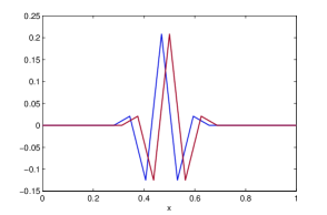
Figure 1: Wavelet functions taken from a basis (left) and a dictionary (right) corresponding to a linear spline-wavelet prototype from [11].

Algorithm 2 constructs a discrete dictionary, i.e., a matrix $\mathbf{D}^{W}$ which contains values of functions from (26) and (27) at $N_{b}$ equidistant points for some chosen levels determined by the vector $\mathbf{j}$. Since Algorithm 1 enables us to construct values at points of the form $l/2^{u}$, we evaluate functions (26) and (27) at the points

$$x=\frac{l}{2^{r}},\quad l=0,\ldots,N_{b}-1,\quad r=\left\lceil\frac{\log\left(N_{b}-1\right)}{\log\left(2\right)}\right\rceil,$$ (28)

where $\left\lceil y\right\rceil$ denotes the smallest integer number larger than $y$.

For a chosen vector of levels $\mathbf{j}$, we define a vector of indices $\mathbf{ind}$ such that $\text{ind}(1)$ is the number of scaling functions at level $j(1)$, and $\text{ind}(l)$ is the number of wavelets at level $j(l-1)$ for $l=1,\ldots,J$, where $J$ is the length of $\mathbf{j}$. We have

$$\text{supp}\,\phi_{j(1),k,b}=\left[\frac{bk}{2^{j(1)}},\frac{bk+K}{2^{j(1)}}\right],\quad\text{supp}\,\psi_{j,k,b}=\left[\frac{bk}{2^{j}},\frac{bk+\frac{K+M}{2}}{2^{j}}\right].$$ (29)

Comparing the supports of these functions and the interval

$$I=\left[0,\frac{N_{b}-1}{2^{r}}\right]$$ (30)

which contains the points from (28), we find that the number of inner scaling functions, i.e., scaling functions with the whole support in $I$, is

$$n_{i}=\left\lfloor\frac{\left(N_{b}-1\right)\,2^{j(1)-r}-K}{b}\right\rfloor+1,$$ (31)

where the symbol $\left\lfloor y\right\rfloor$ denotes the largest integer number smaller than $y$. The number of left boundary scaling functions, i.e., functions that have only a part of the support in the interior of $I$ and their support contains $0$, is

$$n_{1}=Ka-1,\quad a=1/b,$$ (32)

and similarly the number of right boundary scaling functions is

$$n_{2}=\left\lceil\frac{\left(N_{b}-1\right)\,2^{j(1)-r}}{b}\right\rceil-\left\lfloor\frac{\left(N_{b}-1\right)\,2^{j(1)-r}-K}{b}\right\rfloor-1.$$ (33)

Hence, we have

$$\text{ind}\left(1\right)=n_{1}+n_{i}+n_{2}=Ka-1-\left\lceil\frac{\left(N_{b}-1\right)\,2^{j(1)-r}}{b}\right\rceil.$$ (34)

Similarly, the number of wavelet functions on the level $j(l)$ is

$$\text{ind}\left(1+l\right)=sa-1+\left\lceil\frac{\left(N_{b}-1\right)\,2^{j(l)-r}}{b}\right\rceil.$$ (35)

The first $\text{ind}(1)$ columns of $\mathbf{D}^{W}$ contain values of scaling functions (26), which restricted to $I$ are not identically zero, at points given in (28), i.e.,

$$D^{W}\left(k,l\right)=\phi\left(2^{j(1)}\frac{k-1}{2^{r}}-b\left(l-Ka\right)\right)$$ (36)

for $k=1,\ldots,N_{b}$, $l=1,\ldots,\text{ind}(1)$. The above equation can be recast:

$$D^{W}\left(k,l\right) = \phi\left(\frac{\left(k-1\right)-b\left(l-Ka\right)2^{r-j(1)}}{2^{r-j(1)}}\right)$$

$$= \text{phi}\left(k-b\left(l-Ka\right)2^{r-j(1)}\right),$$

where $\mathbf{phi}$ is defined by (11) for the level $u=r-j(1)$. Using the substitution $m=k-b\left(l-Ka\right)2^{r-j(1)}$, we obtain

$$D^{W}\left(m+b\left(l-Ka\right)2^{r-j(1)},l\right)=\text{phi}(m),\quad m=1,\ldots,K2^{r-j(1)}+1,$$ (38)

under the assumption that $1\leq m+b\left(l-Ka\right)2^{r-j(1)}\leq N_{b}$.

The other columns of $\mathbf{D}^{W}$ contain values of wavelet functions (27) for levels $j=j(1),\ldots,j(J)$ at points (28), i.e.,

$$D^{W}\left(k,n_{p}+l\right)=\psi\left(2^{j}\frac{k-1}{2^{r}}-b\left(l-sa\right)\right),\quad s=\frac{M+K}{2},$$ (39)

for $k=1,\ldots,N_{b}$, $l=1,\ldots,\text{ind}(j+1)$, and $n_{p}=\sum_{p=j(1)}^{j}\text{ind}(p+1-j(1))$. Similarly as above we obtain

$$D^{W}\left(m+b\left(l-sa\right)\,2^{r-j(l)},l+n_{p}\right)=\text{psi}(m),$$ (40)

where $1\leq m+b\left(l-sa\right)2^{r-j(1)}\leq N_{b}$ and $\mathbf{psi}$ is defined by (20) for the level $u=r-j(1)$.

The following procedure WaveletDict computes a wavelet dictionary.

Algorithm 2
Procedure [$\mathbf{D}^{W},\mathbf{ind},\mathbf{col}$] = WaveletDict(namef, $N_{b}$, $\mathbf{j}$, $b$)

  Input: 

namef	name of a wavelet family, for available choices see Appendix A
$N_{b}$	number of points
$\mathbf{j}$	vector of levels
$b$	translation factor $b=2^{-r_{b}}$ for some integer $r_{b}$

  Output: 

$\mathbf{D}^{W}$	wavelet dictionary
$\mathbf{ind}$	$\text{ind}(1)$ is the number of scaling functions at level $j(1)$, and $\text{ind}(k)$ for $k>1$ is the number of wavelets at level $j(k-1)$
$\mathbf{col}$	cell array such that $\text{col}\!\left\{n\right\}=\left\{j,k,\text{type},\text{function}\right\}$ if the $n$-th column of $\mathbf{D}^{W}$ corresponds to values of a scaling function $\phi(2^{j}x-bk)$ or a wavelet $\psi(2^{j}x-bk)$; type=‘inner’ or ‘boundary’ characterizes type of a function; function=‘scaling’ or ‘wavelet’ indicates whether the column corresponds to the values of a scaling function or a wavelet

  {Compute scaling and wavelet filters using Algorithm 8 from Appendix A}

   [$\mathbf{h}$,$\mathbf{g}$,correct_name] = Filters(namef)

  {Test if a wavelet family namef is available}

  if  correct_name$=0$ then

     $\mathbf{D}^{W}=[\,];\,\mathbf{ind}=[\,];\,\mathbf{col}=[\,];\,\text{return}$

  end if

   $K=\text{length}(\mathbf{h})-1$ {support length of $\phi$}

   $s=(K+\text{length}(\mathbf{g})-1)/2$ {support length of $\psi$}

  $r=\left\lceil\log(N_{b}-1)/\log(2)\right\rceil$ {level characterizing $N_{b}$ (c.f. (28)}

  {Remove levels from $\mathbf{j}$ that contain no inner function}

  $j_{min}=\left\lceil\log(s\,2^{r}/(N_{b}-1))/\log(2))\right\rceil$ {coarsest possible level}

   $\mathbf{j}=\mathbf{j}(\mathbf{j}>=j_{min})$ {removing the levels smaller than $j_{min}$} {Test of parameters}

  $d_{j}=\text{length}(\mathbf{j});\quad r_{b}=\left\lceil\log(1/b)/\log(2)\right\rceil$ {parameter $r_{b}$ from $b=1/2^{r_{b}}$}

  if $d_{j}=0$ then

      fprintf(‘no inner functions for these values of levels $\mathbf{j}$, increase $\mathbf{j}$’)

     $\mathbf{D}^{W}=[\,];\,\mathbf{ind}=[\,];\,\mathbf{col}=[\,];\,\text{return}$

  else if $r<\max(\mathbf{j})+r_{b}$ then

      fprintf(‘small number of points $N_{b}$ for these values of $\mathbf{j}$ and $b$’)

     $\mathbf{D}^{W}=[\,];\,\mathbf{ind}=[\,];\,\mathbf{col}=[\,];\,\text{return}$

  end if

  {Compute scaling and wavelet generators using Algorithm 1}

  [$\mathbf{phi},\mathbf{psi}$]=WaveletGen($\mathbf{h},\mathbf{g},r-j(1)$)

   {Compute number of scaling functions at level $j(1)$}

  $\mathbf{ind}=\text{zeros}(d_{j}+1,1)$

  $\text{ind}(1)=Ka-1+\left\lceil(N_{b}-1)\,2^{j(1)-r}/b\right\rceil$ {c.f. (34)}

  {Compute number of wavelets for level $l$}

  for $l=1:d_{j}$ do

     $\text{ind}\left(1+l\right)=sa-1+\left\lceil(N_{b}-1)\,2^{j(l)-r}/b\right\rceil$ {c.f. (35)}

  end for{Compute columns of $\mathbf{D}^{W}$ corresponding to scaling functions}

  $n_{f}=\text{sum}(\mathbf{ind});\,\mathbf{D}^{W}=\text{zeros}(N_{b},n_{f});\,\mathbf{col}=\text{cell}(n_{f},1)$

  $l_{s}=\text{length}(\mathbf{phi});\ n_{1}=Ka-1$ {c.f. (32)}

  $n_{2}=\left\lceil\left(N_{b}-1\right)\,2^{j(1)-r}/b\right\rceil-\left\lfloor\left(\left(N_{b}-1\right)\,2^{j(1)-r}-K\right)/b\right\rfloor-1$ {c.f. (33)}

  {Compute columns corresponding to inner scaling functions (c.f. (38)}

  for $i=n_{1}+1:\text{ind}(1)-n_{2}$ do

     $D^{W}(b(i-Ka)2^{r-j(1)}+1:b(i-Ka)\,2^{r-j(1)}+K\,2^{r-j(1)}+1,i)=\mathbf{phi}$

     $\text{col}\left\{i\right\}=\left\{j(1),\,i-Ka,\,\text{`inner'},\,\text{`scaling'}\right\}$

  end for

  {Compute columns corresponding to boundary scaling functions (c.f. (38)}

  for $i=1:n_{1}$ do

     $D^{W}(1:l_{s}-b\,(n_{1}-i+1)\,2^{r-j(1)},i)=\text{phi}((n_{1}-i+1)\,b2^{r-j(1)}+1:l_{s})$

     $\text{col}\left\{i\right\}=\left\{j(1),-n_{1}+i-1,\text{`boundary'},\,\text{`scaling'}\right\}$

  end for

  for  $i=1:n_{2}$  do

     $p=\text{ind}(1)-n_{2}+i$ {index of column}

     $D^{W}(b\,(p-Ka)2^{r-j(1)}+1:N_{b},p)=\text{phi}(1:N_{b}-b(p-Ka)2^{r-j(1)})$

      $\text{col}\left\{p\right\}=\left\{j(1),-n_{1}+p-1,\text{ `boundary'},\,\text{`scaling'}\right\}$

  end for{Compute columns of $\mathbf{D}^{W}$ corresponding to wavelets (c.f. (40))}

  $n_{p}=\text{ind}(1)$ {number of functions on previous levels}

  for $l=1:d_{j}$ do

     $n_{1}=sa-1$

     $k_{1}=\left\lfloor((N_{b}-1)2^{j(l)-r}-s)/b\right\rfloor,\,k_{2}=\left\lceil((N_{b}-1)2^{j(l)-r)}/b)-1\right\rceil$

      $n_{2}=k_{2}-k_{1};\,n_{f}=n_{1}+n_{2}+k_{1}+1;\,l_{w}=\text{length}(\mathbf{psi})$

     for $i=n_{1}+1:n_{f}-n_{2}$ do

        $D^{W}(b(i-sa)2^{r-j(l)}+1:b(i-sa)2^{r-j(l)}+s2^{r-j(l)}+1,i+n_{p})=\mathbf{psi}$

         $\text{col}\left\{i+n_{p}\right\}=\left\{j(l),i-sa,\text{`inner'},\,\text{`wavelet'}\right\}$

     end for

     for $i=1:n_{1}$ do

        $D^{W}(1:l_{w}-b(n_{1}-i+1)2^{r-j(l)},i+n_{p})=\text{psi}((n_{1}-i+1)b2^{r-j(l)}+1:l_{w})$

         $\text{col}\left\{i+n_{p}\right\}=\left\{j(l),-n_{1}+i-1,\text{`boundary'},\,\text{`wavelet'}\right\}$

     end for

     for $i=1:n_{2}$ do

        $p=n_{f}-n_{2}+i$

         $D^{W}(b(p-sa)2^{r-j(l)}+1:N_{b},p+n_{p})=\text{psi}(1:N_{b}-b(p-sa)2^{r-j(l)})$

        $\text{col}\left\{n_{p}+p\right\}=\left\{j(l),-n_{1}+p-1,\text{`boundary'},\,\text{`wavelet'}\right\}$

     end for

      $\mathbf{psi}=\text{psi}(1:2:\text{length}(\mathbf{psi})),\,n_{p}=n_{p}+\text{ind}(l+1)$

  end for

The main procedure GenDict validates input parameters, generates dictionaries $\mathbf{D}^{W}$ and normalizes their columns.

Algorithm 3
Procedure [$\mathbf{D}^{W},\mathbf{ind},\mathbf{col}$]= GenDict(name,pars)

  Input: 

name	name of a wavelet family, for available choices see Appendix A
pars	parameters in the form pars = $\left\{N_{b},\mathbf{j},b\right\}$

  Description of the parameters:

$N_{b}$	number of points
$\mathbf{j}$	vector of levels
$b$	translation factor $b=2^{-r_{b}}$ for some integer $r_{b}$

  Output: 

$\mathbf{D}^{W}$	wavelet dictionary
$\mathbf{ind}$	$\text{ind}(1)$ is the number of scaling functions at level $j(1)$, and $\text{ind}(k)$ for $k>1$ is the number of wavelets at level $j(k-1)$
$\mathbf{col}$	cell array such that $\text{col}\left\{n\right\}=\left\{j,k,\text{type},\text{function}\right\}$, if the $n$-th column of $\mathbf{D}^{W}$ corresponds to values of scaling function $\phi(2^{j}x-bk)$ or wavelet $\psi(2^{j}x-bk)$; type=‘inner’ or ‘boundary’ characterizes type of a function; function=‘scaling’ or ‘wavelet’ indicates whether the column corresponds to the values of a scaling function or a wavelet

  {Define cell array of names of all available families}

  families= $\left\{\right.$‘CW2’,‘CW3’,‘CW4’,‘CDF97’,‘CDF97d’,‘CDF53’, ‘Short4’,‘Short3’, ‘Short2’, ‘Db3’,‘Db4’,‘Db5’,‘Sym3’,‘Sym4’, ‘Sym5’,‘Coif26’,‘Coif38’$\left.\right\}$

  {Validate input parameters}

  if  $\text{nargin}\neq 2$ then

      error(‘Need 2 input arguments’)

  end if

  if  $\sim\!\text{ischar(namef)}$ then

     error(‘Name must be a string’)

  end if

   $N_{b}=\text{pars}\left\{1\right\};\,\mathbf{j}=\text{pars}\left\{2\right\};\,b=\text{pars}\left\{3\right\};\mathbf{j}=\text{sort}(\mathbf{j})$

  if $b\leq 0$ then

     error(‘I expect $b>0$’)

  end if

   $r=\log(1/b)/\log(2)$

  if $\left|r-\text{round}(r)\right|>10^{-10}$ then

     fprintf(‘Choose $b$ such that $1/b=2^{r}$ for some integer $r$’)

     $\mathbf{D}^{W}=[\,];\,\mathbf{ind}=[\,];\,\mathbf{col}=[\,];\,\text{return}$

  else if ismember($\left\{\text{namef}\right\}$,families)  then

     {Generate dictionary using Algorithm 2}

      [$\mathbf{D}^{W},\mathbf{ind},\mathbf{col}$] = WaveletDict(namef, $N_{b}$, $\mathbf{j}$, $b$)

     {Normalize columns of $\mathbf{D}^{W}$ using Algorithm 9 from Appendix A}

      $\mathbf{D}^{W}$ = NormDict($\mathbf{D}^{W}$,1)

  else

      error(‘Unknown name of a wavelet family’)

  end if

Remark 2.

It is worth remarking that the range of scales, say $\mathbf{j}=\left(j_{0},\ldots,J\right)$ depends on length of the signal partition. For a signal segment of length $N_{b}=2^{r}+1$ a dictionary contains values of scaling functions and wavelets at points $l/2^{r}$ for some integer $r$. For a signal segment of length $2N_{b}-1=2^{r+1}+1$ a dictionary contains values of functions at points $l/2^{r+1}$. Thus we have

$$\phi_{j,k,b}\left(\frac{l}{2^{r}}\right)=\phi\left(2^{j}\frac{l}{2^{r}}-kb\right)=\phi\left(2^{j+1}\frac{l}{2^{r+1}}-kb\right)=\phi_{j+1,k,b}\left(\frac{l}{2^{r+1}}\right)$$ (41)

and

$$\psi_{j,k,b}\left(\frac{l}{2^{r}}\right)\!=\!\psi\left(2^{j}\frac{l}{2^{r}}-kb\right)\!=\!\psi\left(2^{j+1}\frac{l}{2^{r+1}}-kb\right)=\psi_{j+1,k,b}\left(\frac{l}{2^{r+1}}\right).$$ (42)

Therefore, nonzero elements of vectors on the level $j$ in a dictionary for $\mathbb{R}^{N_{b}}$ correspond to nonzero elements of vectors on the level $j+1$ in a dictionary for $\mathbb{R}^{2N_{b}-1}$. This situation is illustrated in Figure 2, where vectors of values $\phi_{j,0,b}\left(l/2^{r}\right)$ are displayed for $j=2$ and $r=4$ and for $j=3$ and $r=5$. Note that the nonzero elements in these vectors are the same. Therefore, if for the signal segment of length $N_{b}$ the vector $\mathbf{j}=\left(j_{0},\ldots,J\right)$ is used, then we recommend to use the vector $\mathbf{j}=\left(j_{0},\ldots,J+1\right)$ for the signal segment of length $2N_{b}-1$, and similarly to use levels $\mathbf{j}=\left(j_{0},\ldots,J+m\right)$ for the signal segment of length $2^{m}N_{b}-1$.

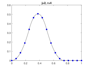
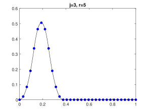
Figure 2: Vectors of values $\phi_{j,0,b}\left(l/2^{r}\right)$ for $j=2$ and $r=4$ (left) and for $j=3$ and $r=5$ (right).

Example 1.

To build dictionaries for the wavelet family ‘Short3’ at levels 2 and 3, for translation parameter $b=1/4$, and the number of points $N_{b}=33$, use the procedure TestDict below.

Algorithm 4 Procedure TestDict

   namef=‘Short3’; $N_{b}=33;\,\mathbf{j}=2:3;\,b=1/4$

   [$\mathbf{D}^{W},\mathbf{ind},\mathbf{col}$]=GenDict(namef,$\left\{N_{b},\mathbf{j},b\right\}$)

The output is the matrix $\mathbf{D}^{W}$ of size $33\times 97$ and the vector $\mathbf{ind}=[27,27,43]$. This means that there are $27$ scaling functions at level 2, 27 wavelets at level 2, and 43 wavelets at level 3. The cell array $\mathbf{col}$ characterizes functions corresponding to columns of $\mathbf{D}^{W}$. For example

$$\text{col}\left\{30\right\}=\left\{2,-9,\text{`boundary'},\text{`wavelet'}\right\}$$ (43)

which means that $30$th column of the matrix $\mathbf{D}^{W}$ contains values of a wavelet function $\psi\left(2^{2}x-b\left(-9\right)\right)$. This wavelet is a boundary wavelet, i.e., only a part of its support lies in the interval $I$ defined by (30). Some of the vectors from this dictionary corresponding to values of scaling functions are displayed in Figure 3 and some of the vectors corresponding to values of wavelets are displayed in Figure 4.

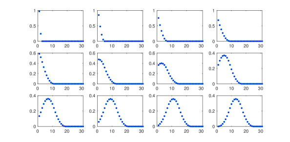
Figure 3: Plots of $12$ vectors from the dictionary $\mathbf{D}^{W}$ from Example 1 corresponding to scaling functions on the level $2$.

Figure 4: Plots of $12$ vectors from the dictionary $\mathbf{D}^{W}$ from Example 1 corresponding to wavelets on the level $2$.

2.4 Construction of dictionaries for ECG modelling

As mentioned in Sec. 1, because ECG signals are usually superimposed to a baseline or smooth background, the full dictionary $\mathbf{D}$ we use for ECG modelling is built as follows

$$\mathbf{D}=[\mathbf{D}^{C}\,\mathbf{D}^{W}],$$ (44)

where $\mathbf{D}^{W}$ is the output of Algorithm 5 and $\mathbf{D}^{C}$ is a matrix containing a few low frequency components from a discrete cosine basis. Before normalization $\mathbf{D}^{C}$ is given as

$$D^{C}(k,n)=\cos(\pi(2k-1)(n-1)/(2N_{b})),\,k=1,\ldots,N_{b},\,n=1,\ldots,M_{c},$$ (45)

where $M_{c}$ is a small number in comparison to $N_{b}$. For the numerical examples of the next section we consider $M_{c}=10$. Algorithm 5 computes $\mathbf{D}^{C}$.

Algorithm 5
Procedure $\mathbf{D}^{C}$ = DCos($N_{b},M_{c}$)

   Input: 

$N_{b}$	the size of the Euclidean space the vectors should belong to
$M_{c}$	number of frequencies to use starting from 0

   Output: 

$\mathbf{D}^{C}$

matrix whos columns are discrete cosine vectors

   $n=1:M_{c};\,k=1:N_{b}$

   $\mathbf{D}^{C}=\cos(\pi(2k-1)^{T}(n-1)/(2N_{b}))$

   $\mathbf{D}^{C}$ = NormDict($\mathbf{D}^{C}$,1)

2.5 Method for construction of the model

In this section we present the procedures for constructing the ECG signal model (c.f. Algorithm 6) and for calculating the assessment metrics. The quality of the signal approximation is assessed with respect to the $\mathrm{PRD}$ defined as follows

$$\mathrm{PRD}=\frac{\|\mathbf{f}-\mathbf{f}^{\rm{r}}\|}{\|\mathbf{f}\|}\times 100\%,$$ (46)

where $\mathbf{f}$ is the original signal and $\mathbf{f}^{\rm{r}}$ is the signal reconstructed by concatenation of the approximated segments $\mathbf{f}^{\rm{a}}\{q\},\,q=1,\ldots,Q$.

The local $\mathrm{PRD}$ with respect to every segment in the signal partition is indicated as ${\mathrm{prd}}(q),\,q=1,\ldots,Q$ and calculated as

$${\mathrm{prd}}(q)=\frac{\|\mathbf{f}\{q\}-\mathbf{f}^{\rm{a}}\{q\}\|}{\|\mathbf{f}\{q\}\|}\times 100\%,\quad q=1,\ldots,Q.$$ (47)

For the signal approximation the OOMP method is stopped through a fixed value $\mathrm{tol}$ so as to achieve the same value of ${\mathrm{prd}}$ for all the segments in the records. Assuming that the target ${\mathrm{prd}}$ before quantization is ${\mathrm{prd}_{0}}$ we set $\mathrm{tol}={\mathrm{prd}_{0}}\|\mathbf{f}_{q}\|/100$.

The goal of the signal model is to approximate each segment in the signal partition using as few atoms as possible. Thus, for a fixed value of $\mathrm{PRD}$, the sparsity of the signal representation is assessed by the sparsity ratio (SR)

$$\text{SR}=\frac{N}{K},$$ (48)

where $N$ is the total length of the signal and $K=\sum_{q=1}^{Q}k(q),$ with $k(q)$ the number of atoms in the atomic decomposition (1) of each segment of length $N_{b}$. The corresponding quantity evaluated for every cell in the partition is the local sparsity ratio

$$\mathrm{sr}(q)=\frac{N_{b}}{k(q)},\quad q=1,\ldots,Q.$$ (49)

This local quantity is relevant to the detection of non-stationary noise, significant distortion in ECG patterns, or changes of morphology in the heart beats.

Given an ECG signal $\mathbf{f}$ the procedure described in Algorithm 6 constructs the signal approximation, $\mathbf{f}^{\rm{r}}$, using the dictionaries introduced in the previous section.

Algorithm 6
Procedure [$\mathbf{f}^{{\rm{r}}},\boldsymbol{\ell},\mathbf{c},{\mathrm{prd}},\mathrm{sr},\mathrm{PRD},\mathrm{SR}$]= SignalModel($\mathbf{f},N_{b},{\mathrm{prd}_{0}},\mathrm{namef},\mathrm{pars},M_{c}$)

   Input:  

$\mathbf{f}$	signal
$N_{b}$	number of points in each segment of the partition
${\mathrm{prd}_{0}}$	parameter to control the approximation error
$\mathrm{namef}$	name of a wavelet family
$\mathrm{pars}$	parameters as described in Algorithm 3
$M_{c}$	number $M_{c}$ of components in the cosine subdictionary

   Output:  

$\mathbf{f}^{{\rm{r}}}$	approximated signal
$\boldsymbol{\ell}$	cell with the indices of the atoms in the atomic decomposition of each element in the partition
$\mathbf{c}$	cell with the coefficients in the atomic decomposition of each element in the partition
${\mathrm{prd}}$	vector ${\mathrm{prd}}\in\mathbb{R}^{Q}$ (cf. (47))
$\mathrm{sr}$	vector $\mathrm{sr}\in\mathbb{R}^{Q}$ (cf. (49))
$\mathrm{PRD}$	global PRD
$\mathrm{SR}$	global SR

  {Create the signal partition using Algorithm 10}

  [$\mathbf{f}^{\rm{c}},Q,\mathbf{f}$]=Partition($\mathbf{f},N_{b}$)

  {Construct the wavelet dictionary $\mathbf{D}^{W}$ using Algorithm 3 given in Appendix B}

  [$\mathbf{D}^{W}$, ind]= GenDict($\mathrm{namef},\mathrm{pars}$)

  {Construct the component $\mathbf{D}^{C}$ using Algorithm 5 given in Appendix B}

  [$\mathbf{D}^{C}$]=DCos($N_{b},M_{c}$)

  {Merge $\mathbf{D}^{C}$ and $\mathbf{D}^{W}$ to create dictionary $\mathbf{D}$}

  $\mathbf{D}=[\mathbf{D}^{C}\,\,\mathbf{D}^{W}]$

  Set $\mathbf{f}^{\rm{r}}=[\;]$, $K=0$ and $N=$length$(\mathbf{f})$.

  for q=1:Q do

     $\mathrm{tol}={\mathrm{prd}_{0}}\|\mathbf{f}^{\rm{c}}\{q\}\|/100$

     {Call the OOMP function to construct the model (c.f. (1))}

     [$\mathbf{f}^{\rm{a}}\{q\},\boldsymbol{\ell}\{q\},\mathbf{c}\{q\}$]=OOMP($\mathbf{f}^{\rm{c}}\{q\},\mathbf{D},\mathrm{tol},1$)

     {Calculate local sr and prd (c.f. (49) and (47)}

     ${\mathrm{prd}}(q)=\frac{\|\mathbf{f}^{\rm{c}}\{q\}-\mathbf{f}^{\rm{a}}\{q\}\|}{\|\mathbf{f}^{\rm{c}}\{q\}\|}\times 100$

     $k(q)=\text{length}(\mathbf{c}\{q\}))$

     $\mathrm{sr}(q)=N_{b}/k(q)$

     $K=K+k(q)$

     $\mathbf{f}^{\rm{r}}=[\mathbf{f}^{\rm{r}}\,\mathbf{f}^{\rm{a}}\{q\}]$

  end for

  {Calculate global SR and PRD (c.f. (48) and (46))}

  $\mathrm{SR}=N/K$; $\mathrm{PRD}=\frac{\|\mathbf{f}-\mathbf{f}^{\rm{r}}\|}{\|\mathbf{f}\|}\times 100$

3 Results

We illustrate now the use of the software to approximate records 117, 202, and 231 in the MIT-BIH Arrhythmia database. Each record consists of 650000 samples and is partitioned for the approximation in segments of $N_{b}=500$ points each. Table 1 gives the values of the SR (c.f. (48)) achieved using wavelet bases, denoted as $\mathrm{SR}_{\mathrm{B}}$, and wavelet dictionaries denoted as $\mathrm{SR}_{\mathrm{D}}$. The wavelet families are indicated in the first column of Table 1. The wavelet dictionary is constructed with scales $\mathbf{j}=\left(3,\ldots,7\right)$ and translation parameter $b=1/4$, whilst the wavelet basis entails to add one more scale and a translation parameter $b=1$. In all the cases the approximation is realized to obtain $\mathrm{PRD}=0.51\%$.

Table 1 is produced by running the script ‘Run_ECG_Appox’ and changing the variable ‘namef’ to the corresponding family option.

Algorithm 7 Procedure Run_ECG_Approx

  {Read the signal $\mathbf{f}$}

  file=‘Record_231_11bits.dat’

  fid=fopen(file,‘r’)

  $\mathbf{f}$=fread(fid,‘ubit11’)

  fclose(fid)

  {Set the required PRD for the approximation}

  ${\mathrm{prd}_{0}}=0.53$

  {Set the length for each segment in the signal partition}

  $N_{b}=500$

  {Set the parameters for the wavelet dictionary}

  $\mathrm{namef}=$‘CDF97’; $b=0.25;\,\mathbf{j}=3:7;\,\mathrm{pars}=\{N_{b},\mathbf{j},b\}$

  {Set the number of cosine components}

  $M_{c}=10$

  {Construct the signal module}

  [$\mathbf{f}^{{\rm{r}}},\boldsymbol{\ell},\mathbf{c},{\mathrm{prd}},\mathrm{sr},\mathrm{PRD},\mathrm{SR}$]= SignalModel($\mathbf{f},N_{b},{\mathrm{prd}_{0}},\mathrm{namef},\mathrm{pars},M_{c}$)

  {Plote the first 2000 sample points in the signal, the approximation and the error}

Table 1: SRs achieved using dictionaries with $\mathbf{D}^{W}$ component as indicated in the first column of the table. $\mathrm{SR}_{\mathrm{B}}$ are values of SR obtained if $\mathbf{D}^{W}$ is a basis and $\mathrm{SR}_{\mathrm{D}}$ if $\mathbf{D}^{W}$ is a dictionary.

Rec.	117		202		231
$\mathbf{D}^{W}$	$\mathrm{SR}_{\mathrm{B}}$	$\mathrm{SR}_{\mathrm{D}}$	$\mathrm{SR}_{\mathrm{B}}$	$\mathrm{SR}_{\mathrm{D}}$	$\mathrm{SR}_{\mathrm{B}}$	$\mathrm{SR}_{\mathrm{D}}$
$\mathbf{CW2}$	17.5	26.5	17.3	24.5	15.7	23.0
$\mathbf{CW3}$	17.4	28.1	15.9	24.9	15.6	24.0
$\mathbf{CW4}$	15.7	24.8	14.3	22.5	18.4	21.9
$\mathbf{CDF97}$	21.5	30.3	21.4	28.4	19.5	27.5
$\mathbf{CDF97d}$	17.2	23.5	17.3	22.5	15.8	21.9
$\mathbf{CDF53}$	22.4	29.6	23.6	27.0	20.2	27.0
$\mathbf{Db3}$	18.5	23.7	18.1	22.7	16.6	22.7
$\mathbf{Db4}$	19.0	25.7	19.1	24.7	17.7	24.1
$\mathbf{Db5}$	20.4	26.1	18.7	24.2	17.8	24.1
$\mathbf{Sym3}$	18.4	23.8	18.1	22.7	16.6	22.7
$\mathbf{Sym4}$	19.7	27.5	19.5	25.8	17.7	25.1
$\mathbf{Sym5}$	20.5	28.3	20.6	28.5	18.4	25.4
$\mathbf{Short2}$	8.2	27.9	8.7	26.3	8.1	24.7
$\mathbf{Short3}$	19.6	31.8	18.3	27.6	17.8	27.3
$\mathbf{Short4}$	9.5	29.1	10.1	27.6	9.1	26.6
$\mathbf{Coif26}$	17.7	23.0	17.7	21.8	16.3	24.7
$\mathbf{Coif38}$	19.5	28.5	19.7	26.5	17.8	26.1

The top left graph in Figure 5 illustrates the first 2000 points in the record 231 and the approximation for $\mathrm{PRD}=0.51\%$. The top right graph represents the values of local sparsity $1/\mathrm{sr}(q)$, $q=1,\ldots,1300$ for the same record. It is noticed that these values can be classified into two well defined bands. The bottom left graph in Figure 5 shows a typical heart beat in a frame corresponding to a value $1/\mathrm{sr}$ in the upper band, and the bottom right graph to a value in the lower band. The morphologic difference between the two heart beats is noticeable at a glance.

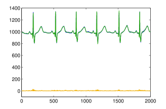
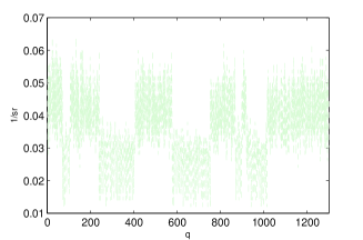
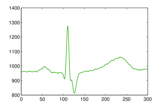
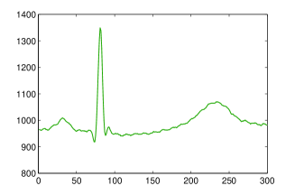
Figure 5: The waveforms in the top left graph are the raw data and the approximations corresponding to 2000 points in the records 231 (the bottom line in the same graph is the point-wise error). The top right graph plots the values $1/\mathrm{sr}$ for records 231. The bottom left graph is a typical heart beat in a segment for which the values of $1/\mathrm{sr}(q)$ belongs to the upper band. In the bottom right graph the heart beat corresponds to a frame in the lower band.

4 Discussion

As observed in the Table 1, the gain in dimensionality reduction (larger value of SR) is significant when considering a wavelet dictionary, instead of a wavelet basis, as component $\mathbf{D}^{W}$ of the full dictionary $\mathbf{D}$. This result was demonstrated in [32] on the whole MIT-BIH Arrhythmia database, which motivated the present work to provide the details and algorithms for the actual construction of dictionaries from different wavelet prototypes. Notice that dictionaries for the families CDF97, CDF53, and Short3 produce the highest sparsity ratios. This is also in line with the results presented in [32] for the MIT-BIH Arrhythmia data set.

In [32] wavelet dictionaries have been shown to be suitable for lossy compression at low level distortion. However, dimensionality reduction is also useful for other applications. It is envisaged that the model could be relevant to analysis and classification tasks [31].

While the results have been obtained using the OOMP approach for selecting the elementary components in the model, other selection strategies [18, 19, 27, 34] could be applied with the identical dictionaries. The focus of this work was the construction of dictionaries delivering piecewise sparse approximation of ECG signals using any suitable approach for the selection process.

5 Conclusions

A detailed description of methods, algorithms, and usage of the software for the construction of wavelet dictionaries has been presented. The use of the software, which has been made publicly available on a dedicated website [15], was illustrated to reduce the dimensionality of three records from the MIT-BIH Arrhythmia database. For all the wavelet families, the sparsity ratio yielded by dictionaries with translation parameter $b=1/4$ was shown to be significantly larger than for the corresponding wavelet bases. The conclusions coincide with those that were drawn in the previous publication [32] using the whole database. The purpose of this paper was to provide a complete description of the construction of the wavelets dictionaries, which had not been addressed in [32]. We believe the proposed dictionaries should be of assistance to general applications which relay on dimensionality reduction, at low level distortion, as a first step of further ECG signal processing.

Declaration of Competing Interest

There are no known conflicts of interest associated with this publication.

Statement of Ethical Approval

Ethical approval is not required for this work.

Appendix A

In this appendix, we present auxiliary procedures used in algorithms in Section 2. In the algorithms, ‘namef’ denotes a name of a wavelet family, available choices are:

namef=	‘CW2’	Chui-Wang linear spline wavelets [11]
=	‘CW3’	Chui-Wang quadratic spline wavelets [11]
=	‘CW4’	Chui-Wang cubic spline wavelets [11]
=	‘CDF97’	primal CDF97 wavelets [6]
=	‘CDF97d’	dual CDF97 wavelets [6]
=	‘CDF53’	primal CDF53 wavelets [6]
=	‘Short4’	cubic spline wavelet with short support and 4 vanishing moments [9, 20]
=	‘Short3’	quadratic spline wavelet with short support and 3 vanishing moments [9, 20]
=	‘Short2’	linear spline wavelet with short support and 2 vanishing moments [9, 20]
=	‘Db3’	Daubechies wavelet with 3 vanishing moments [16]
=	‘Db4’	Daubechies wavelet with 4 vanishing moments [16]
=	‘Db5’	Daubechies wavelet with 5 vanishing moments [16]
=	‘Sym3’	symlet with 3 vanishing moments [17]
=	‘Sym4’	symlet with 4 vanishing moments [17]
=	‘Sym5’	symlet with 5 vanishing moments [17]
=	‘Coif26’	coiflet with 2 vanishing moments and the support length 6 that is most regular [17]
=	‘Coif38’	coiflet with 3 vanishing moments and the support length 8 that is most symmetrical [17]

A wavelet basis is determined by its scaling and wavelet filters. Algorithm 8 assigns these filters for a chosen wavelet family, the values of filters are computed by methods from [6, 9, 11, 12, 16, 17, 20].

Algorithm 8
Procedure [$\mathbf{h}$,$\mathbf{g}$,correct_name] = Filters(namef)

   Input:  

namef

name of a wavelet family

   Output:  

$\mathbf{h}$	scaling filter for a wavelet family specified by ‘namef’
$\mathbf{g}$	wavelet filter for a wavelet family specified by ‘namef’
correct_name	returns $1$ if ‘namef’ is a name of an available wavelet family, otherwise returns $0$

   correct_name=1

  switch (namef)

  case ‘CW2’:

      $\mathbf{h}=[1/2,1,1/2];\,\mathbf{g}=[1,-6,10,-6,1]/12$

  case ‘CW3’ :

      $\mathbf{h}=[1/4,3/4,3/4,1/4];\,\mathbf{g}=[1,-29,147,-303,303,-147,29,-1]/480$

  case ‘CW4’ :

      $\mathbf{h}=[1/8,1/2,3/4,1/2,1/8]$

      $\mathbf{g}=[1,-124,1677,-7904,18482,-24264,18482,-7904,1677,-124,1]/2520$

  case ‘CDF97’:

      $\mathbf{h}=[-0.045635881557,-0.028771763114,0.295635881557,0.557543526229,$ $0.295635881557,-0.028771763114,-0.045635881557]$

      $\mathbf{g}=[0.026748757411,0.016864118443,-0.078223266529,-0.266864118443$ $0.602949018236,-0.266864118443,-0.078223266529,0.016864118443,$ $0.026748757411]$

  case ‘CDF97d’:

     $\mathbf{h}=[0.026748757411,-0.016864118443,-0.078223266529,0.266864118443,$$0.602949018236,0.266864118443,-0.078223266529,-0.016864118443,$ $0.026748757411000]$

     $\mathbf{g}=[0.045635881557,-0.028771763114,-0.295635881557,0.557543526229,$ $-0.295635881557,-0.028771763114,0.045635881557]$

  case ‘CDF53’:

     $\mathbf{h}=[1/2,1,1/2];\,\mathbf{g}=[-1/8,-1/4,3/4,-1/4,-1/8]$

  case ‘Short4’:

     $\mathbf{h}=[1/8,1/2,3/4,1/2,1/8];\,\mathbf{g}=[1/8,-1/2,3/4,-1/2,1/8]$

  case ‘Short3’:

     $\mathbf{h}=[1/4,3/4,3/4,1/4];\,\mathbf{g}=[-1/4,3/4,-3/4,1/4]$

  case ‘Short2’:

      $\mathbf{h}=[1/2,1,1/2];\,\mathbf{g}=[-1/2,1,-1/2]$

  case ‘Db3’ :

      $\mathbf{h}=[0.035226291882101,-0.085441273882241,-0.135011020010391,$ $0.459877502119331,0.806891509313339,0.332670552950957]$

     $\mathbf{g}=[-0.332670552950957,0.806891509313339,-0.459877502119331,$ $-0.135011020010391,0.085441273882241,0.035226291882101]$

  case ‘Db4’:

     $\mathbf{h}=[0.162901714025620,0.505472857545650,0.446100069123190,$ $-0.019787513117910,-0.132253583684370,0.021808150237390,$ $0.023251800535560,-0.007493494665130]$

     $\mathbf{g}=-\text{fliplr}([0.162901714025620,-0.505472857545650,0.446100069123190,$ $0.019787513117910,-0.132253583684370,-0.021808150237390,$ $0.023251800535560,0.007493494665130])$

  case ‘Db5’:

      $\mathbf{h}=[0.003335725285002,-0.012580751999016,-0.006241490213012,$ $0.077571493840065,-0.032244869585030,-0.242294887066190,$ $0.138428145901103,0.724308528438574,0.603829269797473,$ $0.160102397974125]$

      $\mathbf{g}=[-0.160102397974125,0.603829269797473,-0.724308528438574,$ $0.138428145901103,0.242294887066190,-0.032244869585030,$ $-0.077571493840065,-0.006241490213012,0.012580751999016,$ $0.003335725285002]$

  case ‘Sym3’:

      $\mathbf{h}=[0.035226291882101,-0.085441273882241,-0.135011020010391,$ $0.459877502119331,0.806891509313339,0.332670552950957]$

     $\mathbf{g}=[-0.332670552950957,0.806891509313339,-0.459877502119331,$ $-0.135011020010391,0.085441273882241,0.035226291882101]$

  case ‘Sym4’:

     $\mathbf{h}=[0.022785172948000,-0.008912350720850,-0.070158812089500,$ $0.210617267102000,0.568329121705000,0.351869534328000,$ $-0.020955482562550,-0.053574450709000]$

     $\mathbf{g}=\text{fliplr}([0.022785172948000,0.008912350720850,-0.070158812089500,$ $-0.210617267102000,0.568329121705000,-0.351869534328000,$ $-0.020955482562550,0.053574450709000])$

  case ‘Sym5’ :

     $\mathbf{h}=[0.027333068345078,0.029519490925775,-0.039134249302383,$$0.199397533977394,0.723407690402421,0.633978963458212,$ $0.016602105764522,-0.175328089908450,-0.021101834024759,$ $0.019538882735287]$

      $\mathbf{g}=[-0.019538882735287,-0.021101834024759,0.175328089908450,$ $0.016602105764522,-0.633978963458212,0.723407690402421,$ $-0.199397533977394,-0.039134249302383,-0.029519490925775,$ $0.027333068345078]$

  case ‘Coif26’:

     $\mathbf{h}=[9-\sqrt{(}15),13+\sqrt{(}15),6+2\sqrt{(}15),6-2\sqrt{(}15),1-\sqrt{(}15),$ $-3+\sqrt{(}15)]/32$

     $\mathbf{g}=-\text{fliplr}([9-\sqrt{(}15),-13-\sqrt{(}15),6+2\sqrt{(}15),-6+2\sqrt{(}15),$ $1-\sqrt{(}15),3-\sqrt{(}15)]/32)$

  case ‘Coif38’:

     $\mathbf{h}=[-1/32-\sqrt{(}7)/128,-3/128,9/32+3\sqrt{(}7)/128,73/128,9/32-3\sqrt{(}7)/128,-9/128,-1/32+\sqrt{(}7)/128,3/128]$

     $\mathbf{g}=-\text{fliplr}([-1/32-\sqrt{(}7)/128,3/128,9/32+3\sqrt{(}7)/128,-73/128,9/32-3\sqrt{(}7)/128,9/128,-1/32+\sqrt{(}7)/128,-3/128])$

  otherwise

      disp(‘wrong name of a wavelet family’)

      correct_name = 0

  end switch

Now, we introduce a simple procedure NormDict for normalization of dictionaries. More precisely, this procedure normalizes the columns of dictionary $\mathbf{D}$ to have the Euclidean norm equaled to $1/\sqrt{\delta}$.

Algorithm 9
Procedure $\mathbf{D}$ = NormDict($\mathbf{D}$, $\delta$)

   Input:  

$\mathbf{D}$	wavelet dictionary
$\delta$	parameter such that prescribed norm size is $1/\sqrt{\delta}$

   Output:  

$\mathbf{D}$

normalized wavelet dictionary such that the Euclidean norm of each column is $1/\sqrt{\delta}$

  tol=$10^{-5}$

  if nargin=1 then

      $\delta=1$

  end if

  $N$=size($\mathbf{D}$,2); $i=0$

  while  $i<N$  do

      $i=i+1;\,\text{nor}=\sqrt{\delta}\,\left\|D(:,i)\right\|$

     if  $\text{nor}>\text{tol}$  then

         $D(:,i)=D(:,i)/\text{nor}$

     else

         $D(:,i)=[\,];N=N-1$

     end if

  end while

Appendix B

In this appendix, we present auxiliary procedures used in algorithms in Section 2.5. The next procedure Partition creates a partition of the signal $\mathbf{f}$ into $Q$ segments of the prescribed length $N_{b}$.

Algorithm 10
Procedure [$\mathbf{f}^{\rm{c}},Q,\mathbf{f}$]=Partition($\mathbf{f},N_{b}$)

   Input:  

$\mathbf{f}$	signal
$N_{b}$	length of each segment in the partition

   Output:  

$\mathbf{f}^{\rm{c}}$	cells $\mathbf{f}^{\rm{c}}\{q\},\,q=1,\ldots,Q$ with the signal partition
$Q$	number of cells in the partition
$\mathbf{f}$	resized signal to be of length $QN_{b}$

  $N=\text{length($\mathbf{f}$)};Q=\lfloor\frac{N}{N_{b}}\rfloor;t_{o}=1$

  $\mathbf{f}\leftarrow f(1:QN_{b})$

  for $q=1:Q$ do

     $t=t_{o}:t_{o}+N_{b}-1;\,t_{0}=t_{0}+N_{b}$

     $\mathbf{f}^{\rm{c}}\{q\}=f(t)$

  end for

The procedure for signal approximation using OOMP method is presented below.

Algorithm 11
Procedure [$\mathbf{f}^{{\rm{a}}},\boldsymbol{\ell},\mathbf{c}$]= OOMP($\mathbf{f},\mathbf{D},\mathrm{tol},\ell_{1}$)

   Input:  

$\mathbf{f}$	signal to be approximated by an atomic decomposition
$\mathbf{D}$	wavelet dictionary
$\mathrm{tol}$	parameter to control the approximation error
$\ell_{1}$	index of the atom for initializing the OOMP algorithm

   Output:  

$\mathbf{f}^{{\rm{a}}}$	approximation of the signal $\mathbf{f}$ (c.f. (1))
$\boldsymbol{\ell}$	vector whose components are the indices of the selected columns from the input dictionary
$\mathbf{c}$	coefficients $\mathbf{c}\in\mathbb{R}^{N_{b}}$ of the atomic decomposition (c.f. (1))

  {The method implemented in this function is fully described in the main paper [32].}

References

- [1] U.R. Acharya, H. Fujita, M. Adam, S.L. Oh, K.V. Sudarshan, J.H. Tan, J.E.W. Koh, Y. Hagiwara, C.K. Chua, C.K. Poo, R.S. Tan, Automated characterization and classification of coronary artery disease and myocardial infarction by decomposition of ECG signals: A comparative study, Information Sciences 377 (2017) 17–29. doi:https://doi.org/10.1016/j.ins.2016.10.013
- [2] A. Adamo, G. Grossi, R. Lanzarotti, J. Lin, ECG compression retaining the best natural basis k-coefficients via sparse decomposition, Biomedical Signal Processing and Control 15 (2015) 11–17. doi:https://doi.org/10.1016/j.bspc.2014.09.002
- [3] M. Andrle, L. Rebollo-Neira, Cardinal B-spline dictionaries on a compact interval, Applied and Computational Harmonic Analysis 18 (2005) 336–346. doi:10.1016/j.acha.2005.01.001.
- [4] M. Andrle and L. Rebollo-Neira, From cardinal spline wavelet bases to highly coherent dictionaries, Journal of Physics A 41 (2008), article No. 172001. doi:10.1088/1751-8113/41/17/172001.
- [5] A.Y. Hannun, P. Rajpurkar, M. Haghpanahi, G.H. Tison, C. Bourn, M.P. Turakhia, A.Y. Ng, Cardiologist-level arrhythmia detection and classification in ambulatory electrocardiograms using a deep neural network, Nature Medicine 25 (2019) 65–69. doi:https://doi.org/10.1038/s41591-018-0268-3
- [6] A. Cohen, I. Daubechies, J.C. Feauveau, Biorthogonal bases of compactly supported wavelets, Communications on Pure and Applied Mathematics 45 (1992) 485–560. doi:10.1002/cpa.3160450502.
- [7] V.H.C. de Albuquerque, T.M. Nunes, D.R. Pereira, E. J. da Luz, D. Menotti, J. P. Papa, J. M. R. S. Tavareas, Robust automated cardiac arrhythmia detection in ECG beat signals, Neural Computing and Appliccations 29 (2018) 679–693. doi:https://doi.org/10.1007/s00521-016-2472-8.
- [8] A. Cohen, Numerical Analysis of Wavelet methods, Studies in Mathematics and its Applications 32, Elsevier, Amsterdam, 2003.
- [9] D. Chen, Spline wavelets of small support, SIAM Journal on Mathematical Analysis 26 (1995) 500–517. doi:10.1137/S0036141093245264.
- [10] S.S. Chen, D.L. Donoho, M.A. Saunders, Atomic decomposition by basis pursuit, SIAM Journal on Scientific Computing 20 (1998) 33–61. doi:10.1137/S1064827596304010
- [11] C. Chui, J. Wang, On compactly supported spline wavelets and a duality principle, Transactions of the American Mathematical Society 330 (1992) 903–915. doi:10.2307/2153941.
- [12] D. Černá, V. Finěk, K. Najzar, On the exact values of coefficients of coiflets, Central European Journal of Mathematics 6 (2008) 159–169. doi:10.2478/s11533-008-0011-2.
- [13] https://physionet.org/physiobank/database/mitdb/ (Last access July 2019).
- [14] http://www.nonlinear-approx.info/examples/node011.html (Last access July 2019).
- [15] http://www.nonlinear-approx.info/examples/node013.html (Last access July 2019).
- [16] I. Daubechies, Orthonormal bases of compactly supported wavelets, Communications on Pure and Applied Mathematics 41 (1988) 909-996. doi:10.1002/cpa.3160410705
- [17] I. Daubechies, Orthonormal bases of compactly supported wavelets II, variations on a theme, SIAM Journal on Mathematical Analysis 24 (1993) 499-519. doi:10.1137/0524031.
- [18] D.L. Donoho , Y. Tsaig , I. Drori , J.L. Starck, Sparse solution of underdetermined systems of linear equations by stagewise orthogonal matching pursuit, IEEE Transactions on Information Theory 58 (2012) 1094–1121. doi:10.1109/TIT.2011.2173241.
- [19] Y.C. Eldar, P. Kuppinger, H. Bölcskei, Block-sparse signals: uncertainty relations and efficient recovery, IEEE Transactions on Signal Processing 58 (2010) 3042–3054. doi:10.1109/TSP.2010.2044837.
- [20] B. Han, Z. Shen, Wavelets with short support, SIAM Journal on Mathematical Analysis 38 (2006) 530–556. doi:10.1137/S0036141003438374.
- [21] S.J. Lee, J. Kim, M. Lee, A real-time ECG data compression and transmission algorithm for an e-health device, IEEE Transactions on Biomedical Engineering 58 (2011) 2448–2455. doi:10.1109/TBME.2011.2156794.
- [22] H. Li, D. Yuan, X. Ma, D. Cui, L. Cao, Genetic algorithm for the optimization of features and neural networks in ECG signals classification, Scientific Reports 7 (2017), Article No. 41011. doi:10.1038/srep41011
- [23] E. J. Luz, W. Robson Schwartz, G. Camara Chavez, D. Mennotti, ECG-based heartbeat classification for arrhythmia detection: A survey, Computer Methods and Programs in Biomedicine 127 (2016) 144–164. doi: https://doi.org/10.1016/j.cmpb.2015.12.008
- [24] A. Lyon , A. Mincholé, J. P. Martínez, P. Laguna, B. Rodriguez, Computational techniques for ECG analysis and interpretation in light of their contribution to medical advances, Journal of the Royal Society of Interface 15 (2018), article No. 20170821 https://doi.org/10.1098/rsif.2017.0821.
- [25] J.L. Ma, T.T. Zhang, M. C. Dong, A novel ECG data compression method using adaptive Fourier decomposition with security guarantee in e-health applications, IEEE Journal of Biomedical and Health Informatics, 19 (2015) 986–994. doi:10.1109/JBHI.2014.2357841.
- [26] S. G. Mallat, Z. Zhang, Matching Pursuits with Time-Frequency Dictionaries, IEEE Transactions on Signal Processing 41 (1993) 3397–3415. doi:10.1109/78.258082
- [27] D. Needell, J.A. Tropp, CoSaMP: Iterative signal recovery from incomplete and inaccurate samples, Applied and Computational Harmonic Analysis 26 (2009) 301–321. doi:https://doi.org/10.1016/j.acha.2008.07.002
- [28] A. Pandey, B. Singh, S Sain, N. Sood, A joint application of optimal threshold based discrete cosine transform and ASCII encoding for ECG data compression with its inherent encryption, Australasian Physical and Engineering Sciences in Medicine 39 (2016) 833–855. doi:10.1007/s13246-016-0476-4.
- [29] P. Pławiak, Novel methodology of cardiac health recognition based on ECG signals and evolutionary-neural system, Expert Systems with Applications 92 (2018) 334–349. doi:https://doi.org/10.1016/j.eswa.2017.09.022
- [30] Y.C. Pati, R. Rezaiifar, P.S. Krishnaprasad, Orthogonal matching pursuit: recursive function approximation with applications to wavelet decomposition, Proceedings of the 27th Annual Asilomar Conference in Signals, System and Computers, vol 1, (1993) 40–44. doi:10.1109/ACSSC.1993.342465
- [31] S. Raj, K.C. Ray, Sparse representation of ECG signals for automated recognition of cardiac arrhythmias, Expert Systems with Applications 105 (2018) 49–64. doi:https://doi.org/10.1016/j.eswa.2018.03.038
- [32] L. Rebollo-Neira, D. Černá, Wavelet based dictionaries for dimensionality reduction of ECG signals, Biomedical Signal Processing and Control 54 (2019), article No. 101593. doi:https://doi.org/10.1016/j.bspc.2019.101593.
- [33] L. Rebollo-Neira, D. Lowe, Optimized orthogonal matching pursuit approach, IEEE Signal Processing Letters 9 (2002) 137–140. doi:10.1109/LSP.2002.1001652.
- [34] L. Rebollo-Neira, Cooperative greedy pursuit strategies for sparse signal representation by partitioning, Signal Processing 125 (2016) 365–375. doi:10.1016/j.sigpro.2016.02.008.
- [35] L. Rebollo-Neira, Effective high compression of ECG signals at low level distortion, Scientific Reports 9 (2019) article No. 4564. doi:10.1038/s41598-019-40350-x.
- [36] L. Rebollo-Neira, Z. Xu, Sparse signal representation by adaptive non-uniform B-spline dictionaries on a compact interval, Signal Processing 90 (2010) 2308–2313. doi: https://doi.org/10.1016/j.sigpro.2010.02.004
- [37] C. Tan, L. Zhang, H. Wu, A novel Blaschke unwinding adaptive Fourier decomposition based signal compression algorithm with application on ECG signals, IEEE Journal of Biomedical and Health Informatics 23 (2019) 672–682. doi:10.1109/JBHI.2018.2817192.