Models of phase stability in Jackiw-Teitelboim gravity

Abstract

We construct solutions within Jackiw-Teitelboim (JT) gravity in the presence of nontrivial couplings between the dilaton and the Abelian $1$-form where we analyse the asymptotic structure as well as the phase stability corresponding to charged black hole solutions in $1+1$ D. We consider the Almheiri-Polchinski (AP) model as a specific example within $1+1$ D JT gravity which plays a pivotal role in the study of Sachdev-Ye-Kitaev (SYK)/anti-de Sitter (AdS) duality. The corresponding vacuum solutions exhibit a rather different asymptotic structure than their uncharged counterpart. We find interpolating vacuum solutions with AdS₂ in the IR and Lifshitz₂ in the UV with dynamical exponent $z_{\text{dyn}}=3/2$. Interestingly, the presence of charge also modifies the black hole geometry from asymptotically AdS to asymptotically Lifshitz with same value of the dynamical exponent. We consider specific examples, where we compute the corresponding free-energy and explore the thermodynamic phase stability associated with charged black hole solutions in $1+1$ D. Our analysis reveals the existence of a universal thermodynamic feature that is expected to reveal its immediate consequences on the dual SYK physics at finite density and strong coupling.

1 Introduction and Motivations

For the last couple of decades, there had been considerable efforts towards a profound understanding of the underlying non-perturbative dynamics in large $N$ gauge theories using the celebrated AdS/CFT framework [1, 2, 3]. Nonetheless, till date there exists only a few examples where this duality can actually be tested with precise accuracy. In other words, one can exactly solve the spectrum on both sides of the duality albeit they are strongly interacting. In the recent years, an example of this kind has emerged where the spectrum of the $0+1$ dimensional strongly interacting Sachdev-Ye-Kitaev (SYK) model can be solved exactly using large $N$ techniques whose dual counterpart has been conjectured to be the Jackiw-Teitelboim (JT) model in $1+1$ D [4]-[31]. Apart from being exactly solvable, the SYK model exhibits maximal chaos together with an emergent conformal symmetry at low energies which therefore provides a reliable platform to test the holographic correspondence.

For the last couple of years, there has been a systematic effort towards unveiling the dual gravitational counterpart of the SYK model. A hint came from the JT dilaton gravity in $1+1$ D [32]-[36] based on which disparate dual gravity models have been proposed [37]-[44] along with several interesting extensions [45]-[49].

The original SYK/AdS duality deals with Majorana fermions for which neutral dual gravity models are enough to consider. This has been the line of analyses for most of the models so far. However, very recently charged SYK models have been constructed in [50, 52] whose dual gravitational counterpart has been proposed to be given by the 2D effective gravity action of the following form[50],

$$S_{2D}\sim\int d^{2}x\sqrt{-g}\left(\Phi^{2}\mathcal{R}+V(\Phi^{2})-\frac{Z(\Phi^{2})}{4}F^{\mu\nu}F_{\mu\nu}\right).$$ (1)

The last term in the above action (1) represents the non-trivial coupling between the dialton and the Abelian $1$-form. This interaction term can be viewed as an effective coupling which can be obtained as a result of dimensional reduction from the $3+1$ D version of the theory [50]. Eq. (1) without the gauge field is precisely the form of the action considered in [37] with the potential $V(\Phi^{2})$ linear in dilaton. In the present analysis, we choose to work with two specific forms of the dilaton coupling, namely $Z(\Phi^{2})\sim\left(\Phi^{2}\right)^{2}$ and $Z(\Phi^{2})\sim e^{-\Phi^{2}}$ together with the choice of the dilaton potential $V(\Phi^{2})$ as given in [37].

Based on the classical gravity computations, we construct charged 2D black hole solutions in the two aforementioned models. Our analysis reveals that the presence of charge substantially modifies the asymptotic symmetries of the space-time, namely converting it to a two dimensional asymptotic Lifshitz geometry which otherwise would have been an AdS₂ geometry. We further compute the free-energy and explore the thermodynamic phase stability of the obtained solutions. For both the models, we observe a universal thermodynamic feature of phase stability at sufficiently low temperatures and finite density.

The organisation of the paper is as follows: In Section 2, we propose our first model with $Z(\Phi^{2})\sim\left(\Phi^{2}\right)^{2}$. Considering linear potential for the dilaton potential we explore the bounds on the potential which makes the space-time asymptotically AdS. In Sections 3 and 4 we comment on the vacuum structures as well as the black hole solutions both for an asymptotically flat and asymptotically AdS space-time, respectively. In Section 5 we construct perturbative solutions (in charge, $Q$) to our model and analyse the underlying geometry associated to both the vacuum and as well as the charged black hole solutions. This is supplemented with the study of the phase stability of derived solutions using the standard background subtraction method [51]. In Section 6 we repeat our analysis for the exponential dilaton coupling. Finally, we conclude in Section 7 where we mention about the possible implications of our findings on the corresponding SYK counterpart.

2 Example I: Quadratic coupling

We start with the Einstein-Maxwell-dilaton action of the following form,

$$S=-\int d^{2}x\sqrt{-g}\left(\mathcal{R}\Phi^{2}-U(\Phi^{2})-\frac{1}{4}\left(\Phi^{2}\right)^{2}F^{2}\right)-\int dt\sqrt{-\gamma}\;\Phi^{2}\mathcal{K}$$ (2)

where $F=dA$ is the Maxwell 2-form field, $\Phi$ is the dilaton and $U(\Phi^{2})$ is the dilaton potential. Notice that, we have added the the Gibbons-Hawking-York boundary term [53, 54] in the above action, where $\gamma$ is the determinant of the induced metric on the boundary and $\mathcal{K}$ is the trace of the extrinsic curvature [55]. In the subsequent analysis we set the AdS length scale $L=1$ and $16\pi G=1$.

The equations of motion can be written as,

$$0 = \left(\nabla_{\mu}\nabla_{\nu}-g_{\mu\nu}\Box\right)\Phi^{2}+\frac{1}{2}\Phi^{4}\left(F_{\mu\rho}F_{\nu}^{\;\;\rho}-\frac{1}{4}F^{2}g_{\mu\nu}\right)-\frac{1}{2}g_{\mu\nu}U(\Phi^{2})$$ (3a)

$$0 = \mathcal{R}-\frac{F^{2}}{2}\Phi^{2}-\frac{\partial U(\Phi^{2})}{\partial\Phi^{2}}$$ (3b)

$$0 = \partial_{\mu}\left(\sqrt{-g}\Phi^{4}F^{\mu\nu}\right).$$ (3c)

Let us now consider the conformal gauge

$$ds^{2}=-e^{2\omega(x^{+},x^{-})}dx^{+}dx^{-}$$ (4)

where $\displaystyle x^{\pm}=t\pm z$. In this light-cone gauge the equations of motion can be written as,

$$4\partial_{+}\partial_{-}\Phi^{2}-e^{2\omega}U(\Phi^{2})-2\Phi^{4}e^{-2\omega}F_{+-}^{2} = 0$$ (5a)

$$\partial_{\pm}\partial_{\pm}\Phi^{2}-2\left(\partial_{\pm}\omega\right)\left(\partial_{\pm}\Phi^{2}\right) = 0$$ (5b)

$$4\partial_{+}\partial_{-}\omega-\frac{e^{2\omega}}{2}\frac{\partial U(\Phi^{2})}{\partial\Phi^{2}}+2e^{-2\omega}\Phi^{2}F_{+-}^{2} = 0$$ (5c)

$$\partial_{\pm}\chi = 0$$ (5d)

where we have defined $\chi=\sqrt{-g}\;\Phi^{4}F^{+-}$. Notice that our analysis differs from that of [37] in the sense that there is no fully decoupled equation of motion for $\omega(z)$. As a result we obtain a different solution for the conformal factor $e^{2\omega(z)}$.

In the next step we would like to consider the static solutions. In order to do so, we revert back to the $(t,z)$ coordinates and use the following ansatz for the gauge field,

$$A_{+} =\frac{1}{2}\left(A_{t}+A_{z}\right)\qquad\qquad A_{-}=\frac{1}{2}\left(A_{t}-A_{z}\right)\qquad\qquad A_{\mu}=\left(A_{t},0\right).$$ (6)

In these coordinates (5a)-(5d) can be expressed as,

$$(\Phi^{2})^{\prime\prime}+e^{2\omega}U(\Phi^{2})+\frac{1}{2}\Phi^{4}e^{-2\omega}A_{t}^{\prime 2} = 0$$ (7a)

$$(\Phi^{2})^{\prime\prime}-2\omega^{\prime}(\Phi^{2})^{\prime} = 0$$ (7b)

$$2\omega^{\prime\prime}+e^{2\omega}\frac{\partial U(\Phi^{2})}{\partial\Phi^{2}}-e^{-2\omega}\Phi^{2}A_{t}^{\prime 2} = 0$$ (7c)

$$\Phi^{2}A_{t}^{\prime\prime}-2A_{t}^{\prime}\left(\Phi^{2}\omega^{\prime}-(\Phi^{2})^{\prime}\right) = 0.$$ (7d)

We can rewrite (7a) in the following form

$$U(\Phi^{2})=-e^{-2\omega}\left(\Phi^{2}\right)^{\prime\prime}-\frac{1}{2}\Phi^{4}e^{-4\omega}A_{t}^{\prime 2}.$$ (8)

Let us now consider a constant dilaton profile, $\Phi^{2}(z)=\Phi^{2}_{0}$. In this case substituting (8) in (7c) we obtain

$$2\omega^{\prime\prime}=-2e^{2\omega}\frac{\partial U(\Phi^{2})}{\partial\Phi^{2}}\Bigg{|}_{\Phi^{2}=\Phi^{2}_{0}}.$$ (9)

The Ricci scalar ($\mathcal{R}$) on the other hand, can be written as

$$\mathcal{R}=2\frac{\partial U(\Phi^{2})}{\partial\Phi^{2}}\Bigg{|}_{\Phi^{2}=\Phi^{2}_{0}}.$$ (10)

where we have used (9).

Now, in order for the space-time to have AdS₂ asymptotics we must have the following criteria:

$$\frac{\partial U(\Phi^{2})}{\partial\Phi^{2}}\Bigg{|}_{\Phi^{2}=\Phi^{2}_{0}}<0.$$ (11)

3 Gravity in asymptotically flat $1+1$ D

3.1 Minkowski vacuum

In this section, we would like to consider the vacuum solution corresponding to $1+1$ D dilaton gravity. In order to do so we consider the following metric

$$ds^{2}=-dt^{2}+dz^{2}.$$ (12)

From the gauge equation of motion (3c) we can write

$$F_{tz}=\frac{Q}{\Phi^{4}}.$$ (13)

It is easy to check that the scalar equation of motion (3b) and one of the trace equations of motion corresponding to the metric, (3a), lead to the following form of the dilaton potential,

$$U(\Phi^{2})=-\frac{1}{2}\frac{Q^{2}}{\Phi^{4}}.$$ (14)

On the other hand, the remaining trace equation of motion can be written expressed as,

$$\left(\Phi^{2}\right)^{\prime\prime}+\frac{1}{4}\frac{Q^{2}}{\Phi^{4}}+\frac{1}{2}U(\Phi^{2})=0.$$ (15)

Substituting (14) into (15) we obtain

$$\left(\Phi^{2}\right)^{\prime\prime}=0$$ (16)

whose solution may be written as,

$$\Phi^{2}=bz+a$$ (17)

where $a$ and $b$ are arbitrary integration constants.

3.2 Charged black hole solutions

We choose to work with metric ansatz of the following form,

$$ds^{2}=-f(z)dt^{2}+f^{-1}(z)dz^{2}.$$ (18)

The only component of the Maxwell field strength tensor can thus be written as

$$F_{tz}=\frac{Q}{\Phi^{4}(z)}$$ (19)

where $Q$ is an integration constant which we can identify as the charge of the black hole, and we have used (3c) in order to derive (19).

With the metric (18) the remaining equations of motion (3a) and (3b) can be wriiten as,

$$f^{\prime}(z)\left(\Phi^{2}\right)^{\prime}+\frac{Q^{2}}{2\left(\Phi^{2}\right)^{2}}+U(\Phi^{2}) =0$$ (20)

$$2f(z)\left(\Phi^{2}\right)^{\prime\prime}+f^{\prime}(z)\left(\Phi^{2}\right)^{\prime}+\frac{Q^{2}}{2\left(\Phi^{2}\right)^{2}}+U(\Phi^{2}) =0$$ (21)

$$f^{\prime\prime}(z)-\frac{Q^{2}}{\Phi^{6}(z)}+\frac{\partial U(\Phi^{2})}{\partial\Phi^{2}} =0.$$ (22)

From (20) and (21) it is easy to check that

$$\left(\Phi^{2}\right)^{\prime\prime}=0$$ (23)

and as a result the dilaton becomes constant at the boundary $z=0$.

As a next step, we determine the metric coefficient $f(z)$ with particular choices of the dilaton potential $U(\Phi^{2})$ where we finally set, $\Phi^{2}=\varphi_{0}=\text{const}$.

Case I: The Almheiri-Polchinski model [37] ($U(\Phi^{2})=C-A\Phi^{2}$) and the Callan-Giddings-Harvey-Strominger (CGHS) model [56] ($U(\Phi^{2})=-A\Phi^{2}$)

From (22) we obtain,

$$f^{\prime\prime}(z)=A+\frac{Q^{2}}{\varphi_{0}^{3}}$$ (24)

whose solution may be written as,

$$\begin{split}f(z)=\left(1-\frac{z}{z_{H}}\right)\left[1-\frac{1}{2}\left(A+\frac{Q^{2}}{\varphi_{0}^{3}}\right)zz_{H}\right].\end{split}$$ (25)

Using (25), the Hawking temperature of the black hole can be obtained as,

$$\begin{split}T_{H}&=\frac{1}{4\pi}\partial_{z}\sqrt{-\frac{g_{tt}}{g_{zz}}}\Bigg{|}_{z=z_{H}}\\ &=\frac{1}{4\pi z_{H}}\left[\frac{1}{2}\left(A+\frac{Q^{2}}{\varphi_{0}^{3}}\right)z_{H}^{2}-1\right].\end{split}$$ (26)

The extremal limit, in which the Hawking temperature vanishes, is characterized by the extremal value of the charge given by,

$$Q_{e}^{2}=\left(\frac{2}{z_{H}^{2}}-A\right)\varphi_{0}^{3}.$$ (27)

On the other hand, by using the Wald formalism, the entropy of the black hole is given by [57],

$$S_{W}=4\pi\Phi^{2}.$$ (28)

The thermodynamic stability of the black hole is determined by computing the corresponding heat capacity ($C$),

$$C=T_{H}\frac{\partial S_{W}}{\partial T_{H}}=\frac{8\pi\varphi_{0}^{4}}{3Q^{2}z_{H}^{2}}\left[1-\frac{1}{2}\left(A+\frac{Q^{2}}{\varphi_{0}^{3}}\right)z_{H}^{2}\right]$$ (29)

where we have used (26) and (28).

For non-extremal black holes one must have $T_{H}>0$ which leads to the following condition,

$$\frac{1}{2}\left(A+\frac{Q^{2}}{\varphi_{0}^{3}}\right)z_{H}^{2}>1.$$ (30)

Substituting (30) in (29) we note that the specific heat is always negative. This suggests that the black holes (25) in an asymptotically flat space-time are indeed unstable and decay through Hawking radiation.

Case II: Magnetic branes [58], $U(\Phi^{2})=\frac{B^{2}}{\Phi^{2}}-A\Phi^{2}$

The equation of motion corresponding to the metric $f(z)$ can be expressed as,

$$f^{\prime\prime}(z)=A+\frac{B}{\varphi_{0}^{2}}+\frac{Q^{2}}{\varphi_{0}^{3}}$$ (31)

where we have used (22). The general solution to the above equation (31) is given by,

$$\begin{split}f(z)=\left(1-\frac{z}{z_{H}}\right)\left[1-\frac{1}{2}\left(A+\frac{B}{\varphi_{0}^{2}}+\frac{Q^{2}}{\varphi_{0}^{3}}\right)zz_{H}\right].\end{split}$$ (32)

Proceeding in the same line of analysis as in the previous Case I, the thermodynamic quantities may be found as follows:

• The Hawking temperature:

  $$T_{H}=\frac{1}{4\pi z_{H}}\left[\frac{1}{2}\left(A+\frac{B}{\varphi_{0}^{2}}+\frac{Q^{2}}{\varphi_{0}^{3}}\right)z_{H}^{2}-1\right].$$ (33)

• Extremal value of charge:

  $$Q_{e}^{2}=\left[\frac{2}{z_{H}^{2}}-\left(A+\frac{B}{\varphi_{0}^{2}}\right)\right]\varphi_{0}^{3}.$$ (34)

• The specific heat:

  $$\begin{split}C&=T_{H}\frac{\partial S_{W}}{\partial T_{H}}\\ &=\frac{4\pi\varphi_{0}^{3}}{z_{H}^{2}}\left[1-\frac{1}{2}\left(A+\frac{B}{\varphi_{0}^{2}}+\frac{Q^{2}}{\varphi_{0}^{3}}\right)z_{H}^{2}\right]\left(B+\frac{3Q^{2}}{2\varphi_{0}}\right)^{-1}.\end{split}$$ (35)

  Like in the previous example, it is easy to check that the condition for extremality implies the thermodynamic instability in black holes.

4 Vacuum solutions with AdS₂ asymptotics

Unlike the previous example, here we discuss the possibilities on vacuum solutions with AdS₂ asymptotics. We show that solutions with AdS₂ asymptotics are indeed possible both for the constant as well as the running dilaton profiles.

4.1 Solution with constant dilaton

We first construct solutions with constant dilaton $\Phi^{2}=\Phi_{0}^{2}$.

4.1.1 Case I: $e^{2\omega}=\frac{1}{z^{2}}$

In this case from (7a) we may write

$$A_{t}^{\prime 2}=-\frac{2}{z^{4}\Phi_{0}^{4}}U(\Phi_{0}^{2})$$ (36)

whereas (7b) is satisfied trivially. Notice that, in the above equation $U(\Phi_{0}^{2})$ must be negative. Using the relation $\displaystyle\omega^{\prime}=-\frac{1}{z}$ we can write (7c) as,

$$\frac{2}{z^{2}}+\frac{1}{z^{2}}\frac{\partial U(\Phi^{2})}{\partial\Phi^{2}}\Bigg{|}_{\Phi_{0}^{2}}-z^{2}\Phi_{0}^{2}A_{t}^{\prime 2}=0.$$ (37)

Finally, using (36) we obtain the following relation:

$$\frac{\partial U(\Phi^{2})}{\partial\Phi^{2}}\Bigg{|}_{\Phi_{0}^{2}}=-2\left(1-\frac{|U(\Phi_{0}^{2})|}{\Phi_{0}^{2}}\right)$$ (38)

which leads to the following bound to the potential

$$\frac{|U(\Phi_{0}^{2})|}{\Phi_{0}^{2}}<1.$$ (39)

4.1.2 Case II: $e^{2\omega}=\frac{1}{\sinh^{2}z}$

In this case the equation for the gauge field can be expressed as,

$$A_{t}^{\prime 2}=-\frac{2}{\Phi_{0}^{4}\sinh^{4}z}U(\Phi_{0}^{2})$$ (40)

from which we again conclude that $U(\Phi_{0}^{2})<0$. Substituting $e^{2\omega}$ in (7c) it is trivial to check that one arrives at the same constraint conditions (38) and (39).

4.1.3 Case III: $e^{2\omega}=\frac{1}{\sin^{2}z}$

In this case the equation for the gauge field can be written as,

$$A_{t}^{\prime 2}=-\frac{2}{\Phi_{0}^{4}\sin^{4}z}U(\Phi_{0}^{2})$$ (41)

from which it is evident that $U(\Phi_{0}^{2})<0$. Substituting $e^{2\omega}$ in (7c) we once again arrive at the same constraint conditions (38) and (39).

Thus we observe that the above constraint conditions (38), (39) are universal for all the three cases considered, i.e. they are same irrespective of the choice of the coordinate systems.

4.2 Solutions with running dilaton

Let us consider the metric of the following form,

$$ds^{2}=\frac{1}{z^{2}}\left(-dt^{2}+dz^{2}\right).$$ (42)

With this choice of metric the gauge equation of motion (3c) leads to,

$$F_{tz}=\frac{Q}{\Phi^{4}z^{2}}.$$ (43)

The metric equation of motion can be expressed as,

$$z\left(\Phi^{2}\right)^{\prime}-\frac{1}{4}\frac{Q^{2}}{\Phi^{4}}-\frac{1}{2}U(\Phi^{2}) =0$$ (44)

$$z^{2}\left(\Phi^{2}\right)^{\prime\prime}+z\left(\Phi^{2}\right)^{\prime}+\frac{1}{4}\frac{Q^{2}}{\Phi^{4}}+\frac{1}{2}U(\Phi^{2}) =0.$$ (45)

Substituting (44) into (45) we obtain,

$$z^{2}\left(\Phi^{2}\right)^{\prime\prime}+2z\left(\Phi^{2}\right)^{\prime}=0$$ (46)

whose solution may be formally expressed as,

$$\Phi^{2}=-\frac{b_{1}}{z}+a_{1}.$$ (47)

It is interesting to note that the dilaton diverges near the boundary, $z\approx 0$.

In a similar way, considering the conformal factor as $e^{2\omega}=\sinh^{-2}z,\;\sin^{-2}z$, the solutions to the dilaton can be found as,

$$\Phi^{2} =-b_{2}\coth z+a_{2}$$ (48)

$$\Phi^{2} =-b_{3}\cot z+a_{3},$$ (49)

respectively. Interestingly, both these solutions diverge near the boundary, $z\approx 0$.

Notice that, the divergence of the dilaton profile (47)-(49) near the boundary ($z\approx 0$) is a generic feature of the AdS space-time, see for example [59] and references therein. However, as far as the present analysis is concerned, one of the solutions (47) has an interesting consequence from the perspective of the SYK/AdS duality. One of the interesting facets of this duality is that it allows us to relate the SYK degrees of freedom to the underlying dynamics of the AdS₂ counterpart [11],[42]-[44]. We can consistently set $a_{1}=0$ in (47) by demanding that the dilaton $\Phi^{2}$ vanishes as we probe deep IR ($z\rightarrow\infty$). This observation is in fact consistent with the strongly interacting ($J\sim 1/\Phi^{2}\gg 1$) nature of the dual SYK model in which we are mostly interested [42]-[44]).

5 General solutions: A perturbative approach

In this section, we adopt perturbation techniques in order to find the general solutions to the equations of motion (3a)-(3c) and determine the metric of the space-time. In order to perform our analysis, we consider a running dilaton where the dilaton is a function of $z$ only: $\Phi^{2}=\Phi^{2}(z)$. We also consider the dilaton potential as [37],

$$U(\Phi^{2})=C-A\Phi^{2},\qquad\quad C,A>0.$$ (50)

In order to obtain solutions to the metric as well as the dilaton equations of motion we expand the above entities as a perturbation in the $U(1)$ charge $Q$ namely,

$$\Phi^{2}(z) = \Phi^{2}_{(0)}(z)+Q^{2}\Phi^{2}_{(1)}(z)+\cdots$$ (51a)

$$\omega(z) = \omega_{(0)}(z)+Q^{2}\omega_{(1)}(z)+\cdots$$ (51b)

The Maxwell field strength tensor is given by the solution of (7d) which may be written as,

$$F_{zt}\equiv A_{t}^{\prime}=-\frac{Qe^{2\omega}}{\Phi^{4}(z)}.$$ (52)

On the other hand, the equation of motion for the dilaton (7b) can be recast in the following form

$$(\Phi^{2})^{\prime}=\tilde{C}\;e^{2\omega}$$ (53)

whose solution may be written as,

$$\Phi^{2}(z)=\tilde{C}\int e^{2\omega}dz+\bar{C}$$ (54)

where $\tilde{C}$, $\bar{C}$ are arbitrary integration constants.

In the following we note down the equations of motion upto leading order in the perturbative expansion. Substituting (51b) into (7c) we find,

$$\mathcal{O}(Q^{0}):\qquad 0 =\omega_{(0)}^{\prime\prime}-e^{2\omega_{(0)}}$$ (55)

$$\mathcal{O}(Q^{2}):\qquad 0 =2\omega_{(1)}^{\prime\prime}-4e^{2\omega_{(0)}}\omega_{(1)}-e^{2\omega_{(0)}}\left(\Phi^{2}_{(0)}\right)^{-3}.$$ (56)

On the other hand, substituting (51a) into (7a) we find,

$$\mathcal{O}(Q^{0}):\qquad 0 =\left(\Phi_{(0)}^{2}\right)^{\prime\prime}+2e^{2\omega_{(0)}}\left(1-\Phi_{(0)}^{2}\right)$$ (57)

$$\mathcal{O}(Q^{2}):\qquad 0 =\left(\Phi_{(1)}^{2}\right)^{\prime\prime}-2e^{2\omega_{(0)}}\Phi_{(1)}^{2}+4e^{2\omega_{(0)}}\left[\omega_{(1)}\left(1-\Phi_{(0)}^{2}\right)+\frac{1}{8}\left(\Phi_{(0)}^{2}\right)^{-2}\right].$$ (58)

5.1 Interpolating vacuum solutions

The vacuum solution corresponding to $Q=0$ is characterised by [37]

$$e^{2\omega_{(0)}^{\text{vac}}(z)} =\frac{1}{z^{2}}$$ (59)

$$\Phi_{(0)}^{2^{\text{vac}}}(z) =\left(1+\frac{1}{2z}\right)$$ (60)

which satisfy the zeroth order equations (55) and (57), respectively for the following values of the constants in (54): $\tilde{C}=-1/2$ and $\bar{C}=1$. Thus for the purpose of our present analysis it is sufficient to solve the $\mathcal{O}(Q^{2})$ equations of motion namely, (56) and (58).

Using (56) the solution corresponding to $\omega_{(1)}^{\text{vac}}$ can be expressed as,

$$\omega_{(1)}^{\text{vac}}(z)=\frac{\mathsf{C}_{4}}{z}+\frac{1-2z-4z^{2}+2(1+2z)\cdot\log(1+2z)}{8z(1+2z)}.$$ (61)

Thus the metric for the vacuum can be expressed as,

$$ds^{2}=e^{2\omega_{(0)}}\left(1+2Q^{2}\omega_{(1)}^{\text{vac}}\right)\left(-dt^{2}+dz^{2}\right).$$ (62)

Let us now analyse the IR and UV behaviors of the solution (62).

• In the IR region $z\rightarrow\infty$ the behavior of the metric is given by,

  $$e^{2\omega}\simeq\frac{1}{z^{2}}\left(1-\frac{Q^{2}}{2}\right)+\mathcal{O}\left(z^{-3}\right)$$ (63)

  which thereby leads to an emerging AdS₂ geometry.

• The UV ($z=0$) behavior of the metric is found to be of the following form,

  $$e^{2\omega}\simeq\frac{Q^{2}}{4z^{3}}\left(1+8\mathsf{C}_{4}\right)+\frac{1}{z^{2}}-\frac{2Q^{2}}{3}+\mathcal{O}(z)$$ (64)

  whose leading contribution comes from the first term on the R.H.S of (64). This turns out to be a Lifshitz₂ geometry with dynamical exponent $z_{\text{dyn}}=\frac{3}{2}$.

Thus we observe that the vacuum solution interpolates between Lifshitz₂ in the UV and AdS₂ in the deep IR. It is interesting to note that in the absence of the charge, $Q=0$, the geometry is AdS₂ for both in the IR as well as the UV. Thus we conclude that the presence of the gauge field modifies the UV asymptotics from AdS₂ to Lifshitz₂ [60].

5.2 Charged 2D black holes

The zeroth-order solutions $\Phi^{2}_{(0)}(z)$ and $\omega_{(0)}(z)$ are respectively given by [37],

$$\Phi^{2}_{(0)} = 1+\sqrt{\mu}\coth(2\sqrt{\mu}z)$$ (65a)

$$e^{2\omega_{(0)}} = \frac{4\mu}{\sinh^{2}(2\sqrt{\mu}z)}$$ (65b)

Notice that, in order for the solution (65a) to be consistent with the equations of motion (7a) and (7b) we must choose the constants appearing in (54) as $\tilde{C}=-1/2$ and $\bar{C}=1$.

It is trivial to check that, with the choice of the constants $\tilde{C}$ and $\bar{C}$, (65a) and (65b) are indeed the solutions to the equations of motion (55) and (57). Using (65a) and (65b) in (56) the solution for $\omega_{(1)}^{BH}$ may be written as,

$$\begin{split}&\omega_{(1)}^{BH}(\rho)\\ &=\mathsf{C}_{1}\frac{\rho}{\sqrt{\mu}}+\mathsf{C}_{2}\left[\frac{\rho}{2\sqrt{\mu}}\cdot\log\left(\frac{\sqrt{\mu}+\rho}{\sqrt{\mu}-\rho}\right)-1\right]+\frac{1}{8\mu^{3/2}\left(\mu-1\right)^{2}}\times\\ &\qquad\Bigg{\{}-2\sqrt{\mu}\left(1-\mu\frac{2+\rho}{1+\rho}+\frac{\mu^{2}}{1+\rho}\right)+4\mu^{3/2}\rho\cdot\log(1+\rho)\\ &\qquad-\rho\cdot\log(\rho-\sqrt{\mu})\left(1-3\mu+2\mu^{3/2}\right)+\rho\cdot\log(\rho+\sqrt{\mu})\left(1-3\mu-2\mu^{3/2}\right)\Bigg{\}}\end{split}$$ (66)

where $\mathsf{C}_{1}$, $\mathsf{C}_{2}$ are the integration constants, and we have used the following change in the spatial coordinate [37, 45]

$$z\longrightarrow\frac{1}{2\sqrt{\mu}}\coth^{-1}\left(\frac{\rho}{\sqrt{\mu}}\right).$$ (67)

In the subsequent calculations we set $\mathsf{C}_{2}=0$ in order to obtain a physically meaningful asymptotic structure of the space-time.

Finally, using (51b), (65b) and (66) the metric (4) corresponding to the black hole geometry can be expressed as,

$$\begin{split}ds^{2}&=e^{2\omega}\left(-dt^{2}+dz^{2}\right)\\ &=\frac{4\mu}{\sinh^{2}2\sqrt{\mu}z}\left(1+2Q^{2}\omega_{(1)}^{BH}(z)\right)\left(-dt^{2}+dz^{2}\right)\\ &=4\left(\rho^{2}-\mu\right)\left(1+2Q^{2}\omega_{(1)}^{BH}(\rho)\right)\left(-dt^{2}+\frac{d\rho^{2}}{4\left(\rho^{2}-\mu\right)^{2}}\right).\end{split}$$ (68)

Notice that, the above black hole solution (67) has a horizon at $\rho=\sqrt{\mu}$. On the other hand, the boundary is located at $\rho=\infty$. Expanding the metric near the boundary we find,

$$e^{2\omega(\delta)}\simeq\frac{8Q^{2}\mathsf{C}_{1}}{\sqrt{\mu}\delta^{3}}+\frac{4}{\delta^{2}}-\frac{8Q^{2}\mathsf{C}_{1}\sqrt{\mu}}{\delta}-4\mu+\mathcal{O}(\delta)$$ (69)

where we have changed the variable, $\displaystyle\rho\rightarrow 1/\delta$ and taken the limit $\delta\rightarrow 0$ subsequently. The leading term in the expansion (69) behaves as $\displaystyle\sim\frac{1}{\delta^{3}}$ which is a signature of an asymptotically Lifshitz geometry with dynamical critical exponent $z_{\text{dyn}}=\frac{3}{2}$. It is trivial to check that in the limit $Q^{2}\rightarrow 0$ the resulting metric is that of an asymptotically AdS₂ space-time. Our result thus indicates that in the presence of the gauge field the asymptotic behaviour of the space-time indeed changes from AdS₂ to Lifshitz₂ [60].

Next, we turn our attention towards computing the dilaton profile for our model. Using (54) we observe that,

$$\begin{split}\Phi_{(1)}^{2}&=-\int e^{2\omega_{0}}(z)\omega_{(1)}(z)dz\\ &=2\int\omega_{(1)}(\rho)d\rho.\end{split}$$ (70)

Notice that, in writing the second line we have used (67). Thus the complete solution upto $\mathcal{O}(Q^{2})$ can be expressed as,

$$\begin{split}\Phi^{2}&\simeq\Phi_{(0)}^{2}+Q^{2}\Phi_{(1)}^{2}\\ &=(1+\rho)+2Q^{2}\int\omega_{(1)}(\rho)d\rho.\end{split}$$ (71)

We now compute the thermodynamic quantities corresponding to the above black hole geometry (68). The corresponding Hawking temperature is given by,

$$\begin{split}T_{H}&=\frac{1}{2\pi}\sqrt{-\frac{1}{4}g^{tt}g^{\rho\rho}\left(\partial_{\rho}g_{tt}\right)^{2}}\Bigg{|}_{\rho\rightarrow\sqrt{\mu}}=\frac{\sqrt{\mu}}{\pi}.\end{split}$$ (72)

On the other hand, the Wald entropy associated with the black hole can be found as,

$$\begin{split}S_{W}&=4\pi\left[\left(1+\sqrt{\mu}\right)+2Q^{2}\int\omega_{(1)}(\rho)d\rho\Big{|}_{\rho=\sqrt{\mu}}\right]\\ &=4\pi\left[1+\sqrt{\mu}+Q^{2}\frac{1+4\mathsf{C}_{1}\mu|\mu-1|}{4\sqrt{\mu}|\mu-1|}\right]\end{split}$$ (73)

Notice that (73) is ill defined at $\mu=1$. Therefore one can define black hole solutions for either of the two branches namely, $\mu<1$ or $\mu>1$ which is thereby consistent with the earlier observations [37, 45].

5.3 Phase stability

In order to check whether there is any phase transition/crossover between the empty AdS₂ and the AdS₂ black hole one needs to compare free-energies between different configurations. We substitute (3b) into the action (2) which finally yields,

$$S=-\int d^{2}x\sqrt{-g}\left(\frac{F^{2}}{4}\left(\Phi^{2}\right)^{2}-C\right)-\int dt\sqrt{-\gamma}\;\mathcal{K}\Phi^{2}.$$ (74)

Next we use the equation of motion for the gauge field, (3c) to find the on-shell action as,

$$\begin{split}-S^{(os)}&=-\int d^{2}x\sqrt{-g}\;C+\int d^{2}x\;\partial_{\mu}\left(\sqrt{-g}\;F^{\mu\nu}\left(\Phi^{2}\right)^{2}A_{\nu}\right)\\ &=-C\cdot\text{(Vol)}+\int dt\;\left(\sqrt{-g}\;F^{zt}\left(\Phi^{2}\right)^{2}A_{t}\right)+\int dt\sqrt{-\gamma}\;\mathcal{K}\Phi^{2}\end{split}$$ (75)

where (Vol) is the volume term associated with the following two geometries:

(1) For empty interpolating vacuum we may write down the volume term as,

$$\begin{split}\left(\text{Vol}\right)_{\text{Int}}^{\text{vac}}&=-\int_{0}^{\beta_{0}}d\tau\int_{0}^{\Lambda}d\rho\left(\frac{1}{\rho^{2}}\right)e^{2\omega_{\text{Int}}^{\text{vac}}}(\rho)\\ &=-\beta_{0}\;\mathcal{A}_{\text{vac}}(\rho)\Big{|}_{0}^{\Lambda}\end{split}$$ (76)

where we have used the change of coordinate $\displaystyle z\rightarrow\frac{1}{\rho}$ and

$$\mathcal{A}_{\text{vac}}=\rho-\frac{Q^{2}\rho}{2}\left(1-\frac{\rho}{4}\left(1+8\mathsf{C}_{4}\right)-\frac{\rho}{2}\cdot\log\left(\frac{2+\rho}{\rho}\right)\right).$$ (77)

(2) For the AdS₂ black hole the volume term can be expressed as,

$$\begin{split}\left(\text{Vol}\right)^{BH}&=-\int_{0}^{\beta_{1}}d\tau\int_{\rho\sim\sqrt{\mu}}^{\rho\sim\Lambda}d\rho\frac{1}{2(\rho^{2}-\mu)}e^{2\omega^{\text{BH}}}(\rho)\\ &=-\beta_{1}\;\left(\mathcal{A}^{(\Lambda)}(\rho\rightarrow\Lambda)-\mathcal{A}^{(\mu)}(\rho\rightarrow\sqrt{\mu})\right)\end{split}$$ (78)

where,

$$\begin{split}&\mathcal{A}^{(\Lambda)}(\rho\rightarrow\Lambda)\\ &=\frac{1}{2\mu^{3/2}(\mu-1)^{2}}\Big{\{}2\Lambda\sqrt{\mu}(\mu-1)\Big{[}2\mu(\mu-1)+Q^{2}\left(1+\Lambda\mathsf{C}_{1}\sqrt{\mu}(\mu-1)\right)\Big{]}\\ &\quad+Q^{2}(\Lambda^{2}-\mu)\Big{[}4\mu^{3/2}\cdot\log(1+\Lambda)+(-1+3\mu-2\mu^{3/2})\cdot\log(\Lambda-\sqrt{\mu})\\ &\quad+(1-3\mu-2\mu^{3/2})\cdot\log(\Lambda+\sqrt{\mu})\Big{]}\Big{\}}\end{split}$$ (79)

and

$$\mathcal{A}^{(\mu)}(\rho\rightarrow\sqrt{\mu})=\frac{4\mu(\mu-1)+Q^{2}\Big{[}1+4\mu\mathsf{C}_{1}(\mu-1)\Big{]}}{2\sqrt{\mu}(\mu-1)}.$$ (80)

Here, we have introduced an UV cut-off $\Lambda$ in order to make the integrals finite, and $\beta_{0}$ and $\beta_{1}$ are the periods associated with the interpolating vacuum and the AdS₂ black hole, respectively. Moreover, while $\beta_{1}$ is fixed by (72), $\beta_{0}$ is arbitrary. Thus we can fix $\beta_{0}$ by demanding that at some arbitrary $\rho=\Lambda$, the temperature of both the configurations should be the same namely,

$$\frac{\beta_{0}}{\beta_{1}}=\sqrt{\frac{e^{2\omega^{\text{BH}}}(\rho)}{e^{2\omega_{\text{Int}}^{\text{vac}}}(\rho)}}\Bigg{|}_{\rho\rightarrow\Lambda}.$$ (81)

In the next step, we would like to compute the difference between the volume terms (78) and (76). This may be written in the following form,

$$\begin{split}\Delta\left(\text{Vol}\right)&=-C\left(\left(\text{Vol}\right)^{BH}-\left(\text{Vol}\right)_{\text{Int}}^{\text{vac}}\right)\\ &=C\beta_{1}\Big{[}\left(\mathcal{A}_{1}-\mathcal{B}_{1}\right)\Lambda^{2}+\left(\mathcal{A}_{2}-\mathcal{B}_{2}\right)\Lambda+\left(\mathcal{A}_{3}-\mathcal{B}_{3}\right)-\mathcal{A}^{(\mu)}(\rho\rightarrow\sqrt{\mu})\Big{]}\end{split}$$ (82)

where the individual coefficients are given by

$$\mathcal{A}_{1}=\frac{2Q^{2}\mathsf{C}_{1}}{\sqrt{\mu}},\qquad\quad\mathcal{A}_{2}=2,\qquad\quad\mathcal{A}_{3}=\frac{Q^{2}}{2(\mu-1)}$$ (83)

$$\begin{split}\mathcal{B}_{1}&=\frac{Q^{2}}{\sqrt{2}}\sqrt{\frac{\mathsf{C}_{1}(1+8\mathsf{C}_{4})}{\sqrt{\mu}}}\\ \mathcal{B}_{2}&=\frac{1}{4\sqrt{2}\mathsf{C}_{1}}\sqrt{\frac{\mathsf{C}_{1}}{\sqrt{\mu}(1+8\mathsf{C}_{4})}}\left(\sqrt{\mu}\left(1+8\mathsf{C}_{4}\right)+24\mathsf{C}_{1}\right)\\ \mathcal{B}_{3}&=-Q^{2}\left(1+\mathsf{C}_{1}\sqrt{\mu}\right).\end{split}$$ (84)

It is to be noted that in (84) we have simplified the cumbersome expression for $\mathcal{B}_{3}$ by using the following relation,

$$\mathsf{C}_{1}=\frac{\sqrt{\mu}}{8}\left(1+8\mathsf{C}_{4}\right)$$ (85)

which is easily derived by setting the coefficient of $\Lambda^{2}$ in (82) equal to zero. In addition, using (85), it is easy to check that the coefficient of the $\Lambda$ term in (82) vanishes.

Let us now consider the second term $\Pi$ in (75). Using (52), (68) and (62) this may be written as,

$$\begin{split}\Pi&=Q^{2}\int d\tau\int_{0}^{\Lambda}e^{2\omega_{(0)}(z)}\left(\Phi_{(0)}^{2}(z)\right)^{-2}dz\\ &=\begin{cases}-4\beta_{0}Q^{2}\left(\frac{1}{2+\rho}\right)\Big{|}_{0}^{\Lambda}&\quad\text{(interpolating vacuum)}\\[20.0pt] -2\beta_{1}Q^{2}\left(\frac{1}{1+\rho}\right)\Big{|}_{\sqrt{\mu}}^{\Lambda}&\quad\text{(black hole)}\end{cases}\end{split}$$ (86)

where we have substituted (65a) and (65b). Finally, in the limit $\Lambda\rightarrow\infty$ the difference between the 2^nd terms can be written as,

$$\Delta\left(\Pi\right)=\Pi^{\text{BH}}-\Pi^{\text{vac}}=-2Q^{2}\beta_{1}\left(\frac{1+2\sqrt{\mu}}{1+\sqrt{\mu}}\right).$$ (87)

We now calculate the contribution from the third term $\Sigma$ in (75). In order to do so, we choose a $\rho=\text{Const.}$ hypersurface [55]. Let us now define an outward normal $n^{\rho}$, pointing along the increasing $\rho$, as,

$$g_{\rho\rho}n^{\rho}n^{\rho}=1\qquad\Rightarrow n^{\rho}=\frac{1}{\sqrt{g_{\rho\rho}}}$$ (88)

where $g_{\rho\rho}$ is the metric coefficient in (68) corresponding to the spatial coordinate $\rho$. The trace of the extrinsic curvature, $\mathcal{K}$, can then be written as,

$$\mathcal{K}=n^{\rho}\frac{\partial_{\rho}\sqrt{-\gamma}}{\sqrt{-\gamma}}.$$ (89)

Next, we use (54), (88) and (89) to compute the difference between the third terms in the $\Lambda\rightarrow\infty$ limit. After a few easy steps, we note down this expression as,

$$\begin{split}\Delta\Sigma&=\Sigma^{\text{BH}}-\Sigma^{\text{vac}}\\ &=\frac{\beta_{1}}{8}\Bigg{(}-14Q^{2}+\mu+\frac{\mu}{Q^{4}\mathsf{C}_{1}^{2}}-\frac{\sqrt{\mu}\left(-4+4\mu+Q^{2}\right)}{Q^{2}\mathsf{C}_{1}(\mu-1)}-\frac{\mu}{2\mathsf{C}_{1}^{2}Q^{4}}-\frac{\sqrt{\mu}(Q^{2}-4)}{Q^{2}\mathsf{C}_{1}}\Bigg{)}\end{split}$$ (90)

After performing a long but simple calculation, the difference in the on-shell action can be expressed as,

$$\begin{split}&-\Delta S^{(os)}\\ &=\beta_{1}\Bigg{[}C\Bigg{\{}-2\sqrt{\mu}+Q^{2}\Bigg{(}\frac{1}{2(\mu-1)}+\left(1+\mathsf{C}_{1}\sqrt{\mu}\right)-\frac{\left(1+4\mu\mathsf{C}_{1}(\mu-1)\right)}{2\sqrt{\mu}(\mu-1)}\Bigg{)}\Bigg{\}}\\ &\qquad-2Q^{2}\left(\frac{1+2\sqrt{\mu}}{1+\sqrt{\mu}}\right)+\frac{1}{8}\Bigg{(}-14Q^{2}+\mu+\frac{\mu}{Q^{4}\mathsf{C}_{1}^{2}}-\frac{\sqrt{\mu}\left(-4+4\mu+Q^{2}\right)}{Q^{2}\mathsf{C}_{1}(\mu-1)}\\ &\qquad-\frac{\mu}{2\mathsf{C}_{1}^{2}Q^{4}}-\frac{\sqrt{\mu}(Q^{2}-4)}{Q^{2}\mathsf{C}_{1}}\Bigg{)}\Bigg{]}\end{split}$$ (91)

where we have used the relation (85).

We now analyse the behaviour of the free-energy of the configuration. In the path integral formulation, the free-energy is given by $\displaystyle\Delta\mathcal{F}=-\beta^{-1}\log\mathcal{Z}$ where $\mathcal{Z}$ is the partition function and is defined as$\mathcal{Z}:=e^{-\Delta S^{(os)}}$. Thus the free-energy for the present configuration may be expressed as,

$$\Delta\mathcal{F}:=-\beta_{1}^{-1}\left(-\Delta S^{(os)}\right).$$ (92)

In Fig.1 we present the behaviour of the free-energy $\Delta\mathcal{F}$ between the black hole and the interpolating vacuum as a function of temperature (72). We observe that $\Delta\mathcal{F}<0$ for all values of the temperature $T_{H}\sim\sqrt{\mu}$. The free-energy increases asymptotically for sufficiently small values of temperature and changes its slope at some particular temperature. Afterwards it continues to decrease.

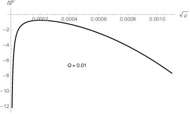
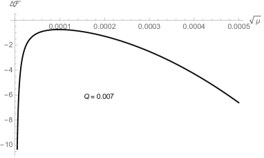
Figure 1: Free energy of the black hole as a function of temperature for different values of charge $Q$. We have taken $\mathsf{C}_{1}=1$, $\mathsf{C}_{2}=0$ and $C=2$.

In Fig.(2), we plot the black hole entropy $\mathcal{S}=\mathcal{S}_{W}=-\frac{\Delta\mathcal{F}}{\Delta\sqrt{\mu}}$ against temperature $T_{H}\sim\sqrt{\mu}$. In these plots the entropy is continuous and increases smoothly as we lower the temperature which rules out the possibility of a first order phase transition. It is to be noted that, this behaviour of entropy is consistent with the Wald entropy of the black hole in (73). This allows us to conclude that the phase diagram corresponding to the parameter space with $\mu<1$ is thermodynamically more preferred than that of the $\mu>1$ branch. We comment on the plausible implications of such phase stabilities on the dual SYK physics in the concluding remarks.

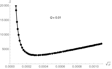
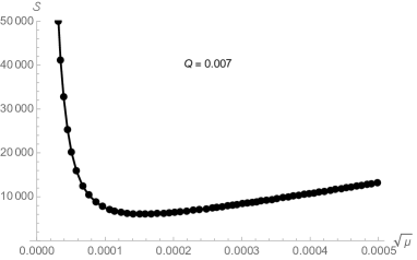
Figure 2: Thermodynamic entropy $\mathcal{S}=-\frac{\Delta\mathcal{F}}{\Delta\sqrt{\mu}}$ of the black hole as a function of temperature $\sqrt{\mu}$ for different values of charge and $\mathsf{C}_{1}=1$, $\mathsf{C}_{2}=0$ and $C=2$.

6 Example II: Exponential coupling

In this section we consider the effective 2D gravity action (1) of the following form,

$$S_{ed}=\int d^{2}x\sqrt{-g}\;\left(\mathcal{R}\Phi^{2}-V(\Phi^{2})-\frac{\lambda}{4}e^{-\Phi^{2}}F_{\mu\nu}F^{\mu\nu}\right)+\int dt\sqrt{-\gamma}\;\Phi^{2}\mathcal{K}$$ (93)

where $\lambda$ is the coupling constant. Also, in our subsequent analysis we shall choose the potential as [37],

$$V(\Phi^{2})=C-A\Phi^{2},\qquad\qquad C,A=2.$$ (94)

The corresponding equations of motion are given by,

$$0 = \left(\nabla_{\mu}\nabla_{\nu}-g_{\mu\nu}\Box\right)\Phi^{2}+\frac{\lambda}{2}e^{-\Phi^{2}}\left(F_{\mu\rho}F_{\nu}^{\;\;\rho}-\frac{1}{4}F^{2}g_{\mu\nu}\right)-\frac{1}{2}g_{\mu\nu}V(\Phi^{2})$$ (95a)

$$0 = \mathcal{R}+\frac{\lambda}{4}e^{-\Phi^{2}}F^{2}-\frac{\partial V(\Phi)}{\partial\Phi^{2}}$$ (95b)

$$0 = \partial_{\mu}\left(\sqrt{-g}e^{-\Phi^{2}}F^{\mu\nu}\right).$$ (95c)

In the next step, using the definition of the metric (4) and the light cone coordinates $\displaystyle x^{\pm}\equiv(t\pm z)$ along with the ansatz (6) we rewrite the above equations of motion as,

$$(\Phi^{2})^{\prime\prime}+e^{2\omega}V(\Phi^{2})+\frac{\lambda}{2}e^{-\Phi^{2}}e^{-2\omega}A_{t}^{\prime 2} = 0$$ (96a)

$$(\Phi^{2})^{\prime\prime}-2\omega^{\prime}(\Phi^{2})^{\prime} = 0$$ (96b)

$$2\omega^{\prime\prime}+e^{2\omega}\frac{\partial V(\Phi^{2})}{\partial\Phi^{2}}+\frac{\lambda}{2}e^{-\Phi^{2}}e^{-2\omega}A_{t}^{\prime 2} = 0$$ (96c)

$$\Phi^{2}A_{t}^{\prime\prime}-A_{t}^{\prime}\left(2\omega^{\prime}+(\Phi^{2})^{\prime}\right) = 0.$$ (96d)

The Maxwell field tensor is the solution to (96d) and can be expressed as,

$$F_{zt}\equiv A_{t}^{\prime}(z)=-Qe^{2\omega}e^{\Phi^{2}}.$$ (97)

Notice that, in the absence of charge ($Q$) the equations of motion correspond to those of the Almheiri-Polchinski model [37]. This allows us to perform a perturbative expansion of the dilaton as well as the metric as done before and find the corresponding vacuum as well as the (charged) black hole solutions.

6.1 Interpolating vacuum solution

In the following, we note down the $\mathcal{O}(Q^{2})$ equations of motion corresponding to the metric as well as the dilaton,

$$0 =2\omega_{(1)}^{\prime\prime}-4e^{2\omega_{(0)}}\omega_{(1)}+\frac{\lambda}{2}e^{2\omega_{(0)}}e^{\Phi_{(0)}^{2}}$$ (98)

$$0 =\left(\Phi_{(1)}^{2}\right)^{\prime\prime}-2e^{2\omega_{(0)}}\Phi_{(1)}^{2}+4e^{2\omega_{(0)}}\left[\omega_{(1)}\left(1-\Phi_{(0)}^{2}\right)+\frac{\lambda}{8}e^{\Phi_{(0)}^{2}}\right]$$ (99)

while $\mathcal{O}(1)$ solutions are given by (59) and (60).

The solution to (98) can be found as,

$$\omega_{(1)}(z)=\frac{\mathsf{C}_{5}}{z}-\frac{\lambda}{24z}\left(-2ze^{1+1/2z}\left(1+2z-4z^{2}\right)+e\;\text{Ei}\left(\frac{1}{2z}\right)\right)$$ (100)

where the exponential integral function is given by,

$$\text{Ei}(z)=-\mathcal{P}\int_{-z}^{\infty}dt\frac{e^{-t}}{t}.$$ (101)

Finally, we express the metric (4) as,

$$ds^{2}=e^{2\omega_{(0)}(z)}\left(1+2Q^{2}\omega_{(1)}(z)\right)\left(-dt^{2}+dz^{2}\right)$$ (102)

The behaviour of the metric (4) in the IR ($z\rightarrow\infty$) is obtained as,

$$e^{2\omega(z)}\Big{|}_{z\rightarrow\infty}\simeq-\frac{2}{3}e\lambda Q^{2}+\frac{1}{z^{2}}\left(1+\frac{1}{4}e\lambda Q^{2}\right)+\mathcal{O}\left(\frac{1}{z^{3}}\right)$$ (103)

which clearly indicates that the IR behaviour of the geometry is AdS₂. On the other hand, near the boundary ($z\approx 0$) the metric (4) behaves as,

$$e^{2\omega(z)}\Big{|}_{z\approx 0}\simeq\frac{2Q^{2}\mathsf{C}_{5}}{z^{3}}+\frac{1}{z^{2}}+e^{1/2z}\frac{1}{\mathcal{O}(z)}+\mathcal{O}(1)$$ (104)

whose leading order term is $\sim 1/z^{3}$ which is a signature of an asymptotically Lifshitz space-time with dynamical scaling exponent $z_{\text{dyn}}=3/2$. Thus the geometry interpolates between AdS₂ in the IR and Lifshitz₂ in the UV. This observation is similar in spirit to what we have found in the earlier example.

6.2 Black hole solution

In order to obtain the charged black hole solution we recall the corresponding zeroth order solutions (65a) and (65b) and substitute them into (99) which finally yields the first order correction to the metric,

$$\begin{split}&\omega_{(1)}(\rho)\\ &=\mathsf{C}_{6}\frac{\rho}{\sqrt{\mu}}+\mathsf{C}_{7}\Bigg{[}-1+\frac{\rho}{\sqrt{\mu}}\cdot\log\sqrt{\frac{\sqrt{\mu}+\rho}{\sqrt{\mu}-\rho}}\;\Bigg{]}\\ &-\frac{\lambda e^{1-\sqrt{\mu}}}{8\mu\sqrt{\mu}}\Big{[}-2\sqrt{\mu}e^{\rho+\sqrt{\mu}}+\rho e^{2\sqrt{\mu}}\left(\sqrt{\mu}-1\right)\text{Ei}(\rho-\sqrt{\mu})+\rho\left(\sqrt{\mu}+1\right)\text{Ei}(\rho+\sqrt{\mu})\Big{]}\end{split}$$ (105)

where $\mathsf{C}_{6}$ and $\mathsf{C}_{7}$ are arbitrary integration constants and $\text{Ei}(z)$ is given in (101). Notice that, in finding the above solution we have used the change in coordinate (67).

Finally, using (51b) we note down the metric (4),

$$\begin{split}ds^{2}&=e^{2\omega}\left(-dt^{2}+dz^{2}\right)\\ &=4\left(\rho^{2}-\mu\right)\left(1+2Q^{2}\omega_{(1)}^{BH}(\rho)\right)\left(-dt^{2}+\frac{d\rho^{2}}{4\left(\rho^{2}-\mu\right)^{2}}\right).\end{split}$$ (106)

Clearly, in this coordinates the horizon of the black hole is located at $\rho=\sqrt{\mu}$. On the other hand, the behaviour of the metric (106) near the boundary $\rho\rightarrow\infty$ may be found as,

$$e^{2\omega}(\rho)\Big{|}_{\rho\rightarrow\frac{1}{\Delta}}\simeq\frac{e^{\frac{1}{\Delta}}}{\mathcal{O}(\Delta)}+\frac{8Q^{2}\mathsf{C}_{6}}{\sqrt{\mu}\Delta^{3}}+\frac{4}{\Delta^{2}}+\frac{1}{\mathcal{O}(\Delta)}$$ (107)

where we have set $\mathsf{C}_{7}=0$ in order to obtain physical boundary conditions in the asymptotic limit of the metric. Referring to (107), we may conclude that the geometry is asymptotically Lifshitz near the boundary of the space-time with dynamical exponent $z_{\text{dyn}}=3/2$. This observation is similar to that observed in Section 5.2.

6.3 Free-energy and phase stability

In order to understand the underlying phase structure associated with the black hole solution (106) we follow the same line of analysis as in Section 5.3. The on-shell action for the present model may be calculated as,

$$\begin{split}-S^{(os)}_{ed}&=C\int d^{2}x\sqrt{-g}+\frac{\lambda}{2}\int d^{2}x\;\partial_{\mu}\left(\sqrt{-g}e^{-\Phi^{2}}\left(1+\Phi^{2}\right)F^{\mu\nu}A_{\nu}\right)\\ &\qquad-\frac{\lambda}{2}\int d^{2}x\;\partial_{\mu}\left(\sqrt{-g}e^{-\Phi^{2}}\Phi^{2}F^{\mu\nu}\right)A_{\nu}-\int dt\;\sqrt{-\gamma}\mathcal{K}\Phi^{2}.\end{split}$$ (108)

The Abelian $1$-form in (108) may be replaced as,

$$A_{t}=-Q\int dz\;e^{2\omega_{(0)}}e^{\Phi_{(0)}^{2}}\left(1+\mathcal{O}(Q^{2})\right)$$ (109)

where the exponentials in the integrand stand for the zeroth order solutions to the metric and the dilaton.

If we now substitute (97) and (109) into (108) it is easy to check that the second and the third terms in the on-shell action (108) exactly cancel each other. On the other hand, the difference in the volume terms may be schematically expressed as,

$$\begin{split}\Delta\left(\text{Vol}\right)&=C\left(\left(\text{Vol}\right)^{\text{BH}}-\left(\text{Vol}\right)_{\text{Int}}^{\text{vac}}\right)\\ &=-C\beta_{1}\Big{[}\mathcal{D}_{1}-\mathcal{D}_{2}^{(\sqrt{\mu})}-\mathcal{D}_{3}\frac{\beta_{0}}{\beta_{1}}\Big{]}\end{split}$$ (110)

whose finite contribution may be expressed as,

$$\mathcal{D}_{2}^{(\sqrt{\mu})}=\frac{1}{2\sqrt{\mu}}\Big{[}e^{1+\sqrt{\mu}}Q^{2}\lambda+4\mu\left(1+\mathsf{C}_{6}Q^{2}\right)\Big{]}.$$ (111)

Finally, using the definition (92) the corresponding free-energy can be expressed as

$$\Delta\mathcal{F}=-\frac{1}{\pi}\Big{[}e^{1+\sqrt{\mu}}Q^{2}\lambda+4\mu\left(1+\mathsf{C}_{6}Q^{2}\right)\Big{]}$$ (112)

where $\beta_{1}\equiv 1/T_{H}=\pi/\sqrt{\mu}$ is the inverse Hawking temperature of the black hole, which is easily calculated by substituting the metric components of (106) in (72).

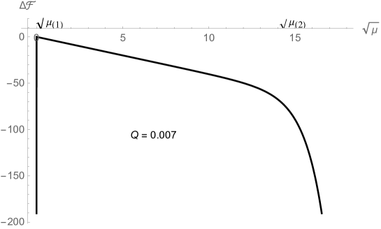
Figure 3: Free energy of the black hole as a function of temperature for $Q=0.007$. We have taken $\mathsf{C}_{6}=1$ and $\mathsf{C}_{7}=0$.

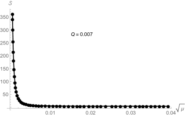
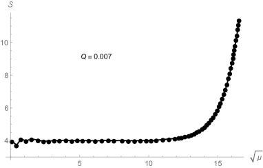
Figure 4: Thermodynamic entropy $\mathcal{S}=-\frac{\Delta\mathcal{F}}{\Delta\sqrt{\mu}}$ of the black hole as a function of temperature $\sqrt{\mu}$. The left panel corresponds to the left-half ($\sqrt{\mu}\in(0,0.04)$) of the corresponding curve in Fig.3 while the right panel shows the remaining right-half of the same curve. Here $Q=0.007$ and $\mathsf{C}_{6}=1$.

We now plot the free-energy ($\Delta\mathcal{F}$) of the black hole against the temperature, $T_{H}\sim\sqrt{\mu}$ (see Fig.3). Further in Fig.4, we show the changes in entropy $\mathcal{S}=S_{W}$ ($=-\Delta\mathcal{F}/\Delta\sqrt{\mu}$) against the temperature $T_{H}\sim\sqrt{\mu}$. From this plot it is evident that there is no first order phase transition as the $\mathcal{S}$-$\sqrt{\mu}$ plot is continuous. We further observe that, this behaviour of entropy is consistent with that of the Wald entropy of the corresponding black hole which can be easily computed using (51a) and (54) and is given by,

$$S_{W}=4\pi\left[1+\sqrt{\mu}+Q^{2}\frac{\lambda e^{1+\sqrt{\mu}}+4\mathsf{C}_{6}\mu}{4\sqrt{\mu}}\right].$$ (113)

From Fig.3 we notice two turning points, $\sqrt{\mu}_{(1)}$ and $\sqrt{\mu}_{(2)}$ ($\sqrt{\mu}_{(1)}<\sqrt{\mu}_{(2)}$) at which the sign of the slope changes. This behaviour is reflected in the corresponding entropy plots in Fig.4 in which the entropy increases asymptotically both for $\sqrt{\mu}<\sqrt{\mu}_{(1)}$ and $\sqrt{\mu}>\sqrt{\mu}_{(2)}$. In the window $\Delta\sqrt{\mu}\sim\sqrt{\mu}_{(2)}-\sqrt{\mu}_{(1)}$ the entropy does not change considerably. In this window the system falls in the minimum entropy state whose plausible interpretation in terms of SYK degrees of freedom are discussed in the concluding remarks.

7 Concluding remarks

In the present paper, we have proposed models of charged solutions within the framework of $1+1$ D Jackiw-Teitelboim (JT) gravity. Based on our model computations, we have shown that in the presence of non-trivial couplings between the $U(1)$ gauge field and the dilaton the asymptotic geometries get substantially modified both for the vacuum as well as the black hole solutions. In both the examples, the vacuum solutions interpolate between Lifshitz₂ in the UV to AdS₂ in the IR. On the other hand, the black hole solutions turn out to be asymptotically Lifshitz₂ with $z_{\text{dyn}}=3/2$.

We have further analysed the stability of black holes in both the models and observed a universal feature in the free-energy and therefore the entropy of the system. In the first model we have considered the quadratic coupling and in the second model the exponential coupling of the dilaton to the gauge field. In both the cases, at sufficiently low temperatures, we observed a turning point after which the free-energy falls-off sharply (Fig.1 and Fig.3) which corresponds to an increase in the entropy below this temperature (Fig.2 and Fig.4).

The existence of minimal entropy at low temperatures could be interpreted as the formation of the Bose-Einstein like condensate(BEC) in the dual SYK model which possibly leads towards superfluid instabilities at low temperatures and finite density [67]. We hope to clarify some of these issues from the perspective of the dual SYK physics in the near future.

Appendix A A note on dimensional reduction

In this section, we propose a dimensional reduction procedure in order to show that our $1+1$ D dilaton gravity models (2) and (93) are indeed effective models of a higher dimensional gravity theory.

Let us consider the following $2+1$ D Einstein-dilaton gravity,

$$S_{3D}=\int d^{3}x\sqrt{-g^{(3)}}\left(\mathcal{R}^{(3)}+\chi(\Psi)+\gamma\left(\partial_{z}\Psi\right)\left(\partial^{z}\Psi\right)\right)$$ (114)

where $\mathcal{R}^{(3)}$ is the three dimensional Ricci scalar and $\chi(\Psi)$ is the dilaton potential which includes the cosmological constant as we see below. Here $\Psi\equiv\Phi^{2}$ of the original analysis.

In order to obtain a $1+1$ D effective action, we dimensionally reduce (114) along the compact direction $\theta$,

$$ds_{(3)}^{2}=ds_{(2)}^{2}+e^{-2\beta\Psi}\left(d\theta+\tilde{A}_{a}dx^{a}\right)^{2}$$ (115)

where $ds_{(2)}^{2}$ is the usual AdS₂ metric (4) with $e^{2\omega}=1/z^{2}$.

Notice that, in (115) the indices $a,b$ run over the uncompactified directions. Also, we have identified $\theta\sim\theta+2\pi$ and assumed an $U(1)$ symmetry for the dilaton field $\Psi$. The gauge fields $\tilde{A}_{a}$ in (115) are known as the Kaluza-Klein vectors. In the subsequent analysis, we choose to work with the ansatz (6).

In the next step, we wish to calculate the $2+1$ D Ricci scalar $\mathcal{R}^{(3)}$ which is related to the $1+1$ D Ricci scalar $\mathcal{R}^{(2)}$ as,

$$\mathcal{R}^{(3)}=\mathcal{R}^{(2)}-\frac{1}{4}e^{-2\beta\Psi}\tilde{F}_{\mu\nu}^{2}+2\beta\left(\partial_{z}\partial^{z}\Psi\right)-2\beta^{2}\left(\partial_{z}\Psi\right)\left(\partial^{z}\Psi\right).$$ (116)

We now find a relation between the determinants of the two metrics as,

$$\sqrt{-g^{(3)}}=\sqrt{-g^{(2)}}e^{-\beta\Psi}.$$ (117)

If we now substitute (116) and (117) in (114), the $2+1$ D action reduces to the following $1+1$ D form,

$$\begin{split}S_{2D}&=\int d^{2}x\sqrt{-g^{(2)}}e^{-\beta\Psi}\left[\mathcal{R}^{(2)}+\chi(\Psi)-\frac{1}{4}e^{-2\beta\Psi}\tilde{F}_{\mu\nu}^{2}\right]\end{split}$$ (118)

where we set $\beta=\pm\sqrt{\gamma/2}$ and $\gamma=2$.

If we redefine $\Psi\rightarrow\log\Psi$ and use $\beta=-1$ in (118) we recover an action which is similar in spirit to the action (2) corresponding to the Model I. Notice that, in order to obtain the desired form of the potential one must set $\chi=\left(A-C/\Psi\right)$ where $A$ plays the role of cosmological constant in the original $2+1$ D gravity model (114). On the other hand, in the limit $\Psi\ll 1$ we obtain an action similar to (93) which corresponds to that of Model II. In this case we set $\beta=-1$ and $\chi\approx-C+(C+A)\Psi$.

Appendix B Black hole solution with $A<0$

In this appendix, we discuss the metric solution corresponding to our first model (2) while considering the linear dilaton potential as $U(\Phi^{2})=C+A\Phi^{2}$. In order to simplify the calculations we choose $A,C=2$.

Using the perturbation expansion (51a) and (51b), we write down the equation of motion (7c) upto leading order in the expansion as,

$$\mathcal{O}(Q^{0}):\qquad 0 =2\omega_{(0)}^{\prime\prime}(z)+2e^{2\omega_{(0)}(z)}$$ (119)

$$\mathcal{O}(Q^{2}):\qquad 0 =2\omega_{(1)}^{\prime\prime}(z)+4e^{2\omega_{(0)}(z)}\omega_{(1)}(z)-\frac{e^{2\omega_{(0)}(z)}}{(\Phi_{(0)}^{2})^{3}}.$$ (120)

Similarly, substituting (51a) and (51b) in the dilaton equation of motion (7a) we obtain,

$$\mathcal{O}(Q^{0}):\qquad 0 =\left(\Phi_{(0)}^{2}\right)^{\prime\prime}+2e^{2\omega_{(0)}}\left(1+\Phi_{(0)}^{2}\right)$$ (121)

$$\mathcal{O}(Q^{2}):\qquad 0 =\left(\Phi_{(1)}^{2}\right)^{\prime\prime}+2e^{2\omega_{(0)}}\Phi_{(1)}^{2}+4e^{2\omega_{(0)}}\left[\omega_{(1)}\left(1+\Phi_{(0)}^{2}\right)+\frac{1}{8}\left(\Phi_{(0)}^{2}\right)^{-2}\right].$$ (122)

The zeroth order equations (119) and (121) have the following solutions,

$$e^{2\omega_{(0)}} =\frac{4\mu}{\cosh^{2}2\sqrt{\mu}z}$$ (123)

$$\left(\Phi_{(0)}^{2}\right) =-\left(1+\sqrt{\mu}\tanh 2\sqrt{\mu}z\right)$$ (124)

Notice that, in obtaining the solution (124) we have set $\bar{C}=-1$ and $\tilde{C}=-\frac{1}{2}$ in (54).

Now, using (51a) and (51b) in (120), the leading order solution $\omega_{(1)}^{BH}$ can be expressed as,

$$\begin{split}&\omega_{(1)}^{BH}(\rho)\\ &=\frac{\rho\mathsf{C}_{8}}{\sqrt{\mu}}+\mathsf{C}_{9}\left[-1+\frac{\rho}{\sqrt{\mu}}\tanh^{-1}\left(\frac{\rho}{\sqrt{\mu}}\right)\right]+\frac{1}{8{\mu-1}^{2}\mu^{3/2}(1+\rho)}\\ &\quad\times\Big{\{}-2\sqrt{\mu}(\mu-1)(-1+\mu-\rho)+\rho(1+\rho)\Big{[}4\mu^{3/2}\cdot\log(1+\rho)\\ &\qquad+\left(-1+3\mu-2\mu^{3/2}\right)\log(\rho-\sqrt{\mu})+\left(1-3\mu-2\mu^{3/2}\right)\log(\rho+\sqrt{\mu})\Big{]}\Big{\}}.\end{split}$$ (125)

where $\mathsf{C}_{8}$, $\mathsf{C}_{9}$ are constants of integration.In writing (125) we have made the following change in the spatial coordinate:

$$z\longrightarrow\frac{1}{2\sqrt{\mu}}\tanh^{-1}\left(\frac{\rho}{\sqrt{\mu}}\right).$$ (126)

Finally, using (51b) and (123), the metric (4) corresponding to the black hole can be written as,

$$\begin{split}ds^{2}=4(\mu-\rho^{2})\left(1+2Q^{2}\omega_{(1)}(\rho)\right)\left(-dt^{2}+\frac{d\rho^{2}}{4(\mu-\rho^{2})^{2}}\right).\end{split}$$ (127)

Clearly, the horizon of the black hole (127) is located at $\rho=\sqrt{\mu}$. However, from the structure of the solution (123) the position of the boundary of the space-time (127) is not quite apparent.

The Hawking temperature corresponding to the above black hole (127) can be written down using the formula (72) and is given by,

$$T_{H}=\frac{\sqrt{\mu}}{2\pi}.$$ (128)

The corresponding Wald entropy can be expressed as,

$$S_{W}=4\pi\left[1+\sqrt{\mu}+Q^{2}\frac{1+4\mathsf{C}_{8}\mu|\mu-1|}{4\sqrt{\mu}|\mu-1|}\right].$$ (129)

Notice that, in writing (129) we have used (51a) and (54).

References

• [1] J. M. Maldacena, “The Large N limit of superconformal field theories and supergravity,” Int. J. Theor. Phys.  38 (1999) 1113 [Adv. Theor. Math. Phys.  2 (1998) 231] doi:10.1023/A:1026654312961, 10.4310/ATMP.1998.v2.n2.a1 [hep-th/9711200].
• [2] E. Witten, “Anti-de Sitter space and holography,” Adv. Theor. Math. Phys.  2 (1998) 253 doi:10.4310/ATMP.1998.v2.n2.a2 [hep-th/9802150].
• [3] O. Aharony, S. S. Gubser, J. M. Maldacena, H. Ooguri and Y. Oz, “Large N field theories, string theory and gravity,” Phys. Rept.  323 (2000) 183 doi:10.1016/S0370-1573(99)00083-6 [hep-th/9905111].
• [4] S. Sachdev and J. Ye, “Gapless spin fluid ground state in a random, quantum Heisenberg magnet,” Phys. Rev. Lett.  70, 3339 (1993) doi:10.1103/PhysRevLett.70.3339 [cond-mat/9212030].
• [5] S. Sachdev, “Holographic metals and the fractionalized Fermi liquid,” Phys. Rev. Lett.  105, 151602 (2010) doi:10.1103/PhysRevLett.105.151602 [arXiv:1006.3794 [hep-th]].
• [6] S. Sachdev, “Strange metals and the AdS/CFT correspondence,” J. Stat. Mech.  1011, P11022 (2010) doi:10.1088/1742-5468/2010/11/P11022 [arXiv:1010.0682 [cond-mat.str-el]].
• [7] A. Kitaev. 2015. A simple model of quantum holography, talk given at KITP strings seminar and Entanglementprogram, February 12, April 7, and May 27, Santa Barbara, U.S.A.
• [8] A. Kitaev. 2014. Hidden correlations in the Hawking radiation and thermal noise, talk given at Fundamental Physics Prize Symposium, November 10, Santa Barbara, U.S.A.
• [9] S. Sachdev, “Bekenstein-Hawking Entropy and Strange Metals,” Phys. Rev. X 5, no. 4, 041025 (2015) doi:10.1103/PhysRevX.5.041025 [arXiv:1506.05111 [hep-th]].
• [10] J. Polchinski and V. Rosenhaus, “The Spectrum in the Sachdev-Ye-Kitaev Model,” JHEP 1604, 001 (2016) doi:10.1007/JHEP04(2016)001 [arXiv:1601.06768 [hep-th]].
• [11] J. Maldacena and D. Stanford, “Remarks on the Sachdev-Ye-Kitaev model,” Phys. Rev. D 94, no. 10, 106002 (2016) doi:10.1103/PhysRevD.94.106002 [arXiv:1604.07818 [hep-th]].
• [12] W. Fu, D. Gaiotto, J. Maldacena and S. Sachdev, “Supersymmetric Sachdev-Ye-Kitaev models,” Phys. Rev. D 95, no. 2, 026009 (2017) Addendum: [Phys. Rev. D 95, no. 6, 069904 (2017)] doi:10.1103/PhysRevD.95.069904, 10.1103/PhysRevD.95.026009 [arXiv:1610.08917 [hep-th]].
• [13] J. Yoon, “Supersymmetric SYK Model: Bi-local Collective Superfield/Supermatrix Formulation,” JHEP 1710, 172 (2017) doi:10.1007/JHEP10(2017)172 [arXiv:1706.05914 [hep-th]].
• [14] A. M. Garcia-Garcia and J. J. M. Verbaarschot, “Spectral and thermodynamic properties of the Sachdev-Ye-Kitaev model,” Phys. Rev. D 94, no. 12, 126010 (2016) doi:10.1103/PhysRevD.94.126010 [arXiv:1610.03816 [hep-th]].
• [15] A. M. Garcia-Garcia and J. J. M. Verbaarschot, “Analytical Spectral Density of the Sachdev-Ye-Kitaev Model at finite N,” Phys. Rev. D 96, no. 6, 066012 (2017) doi:10.1103/PhysRevD.96.066012 [arXiv:1701.06593 [hep-th]].
• [16] A. Jevicki, K. Suzuki and J. Yoon, “Bi-Local Holography in the SYK Model,” JHEP 1607, 007 (2016) doi:10.1007/JHEP07(2016)007 [arXiv:1603.06246 [hep-th]].
• [17] A. Jevicki and K. Suzuki, “Bi-Local Holography in the SYK Model: Perturbations,” JHEP 1611, 046 (2016) doi:10.1007/JHEP11(2016)046 [arXiv:1608.07567 [hep-th]].
• [18] D. J. Gross and V. Rosenhaus, “A Generalization of Sachdev-Ye-Kitaev,” JHEP 1702, 093 (2017) doi:10.1007/JHEP02(2017)093 [arXiv:1610.01569 [hep-th]].
• [19] D. J. Gross and V. Rosenhaus, “The Bulk Dual of SYK: Cubic Couplings,” JHEP 1705, 092 (2017) doi:10.1007/JHEP05(2017)092 [arXiv:1702.08016 [hep-th]].
• [20] A. Kitaev and S. J. Suh, “The soft mode in the Sachdev-Ye-Kitaev model and its gravity dual,” JHEP 1805, 183 (2018) doi:10.1007/JHEP05(2018)183 [arXiv:1711.08467 [hep-th]].
• [21] C. Krishnan, S. Sanyal and P. N. Bala Subramanian, “Quantum Chaos and Holographic Tensor Models,” JHEP 1703, 056 (2017) doi:10.1007/JHEP03(2017)056 [arXiv:1612.06330 [hep-th]];  M. Berkooz, P. Narayan, M. Rozali and J. Simon, “Higher Dimensional Generalizations of the SYK Model,” JHEP 1701, 138 (2017) doi:10.1007/JHEP01(2017)138 [arXiv:1610.02422 [hep-th]].
• [22] C. Peng, M. Spradlin and A. Volovich, “Correlators in the $\mathcal{N}=2$ Supersymmetric SYK Model,” JHEP 1710, 202 (2017) doi:10.1007/JHEP10(2017)202 [arXiv:1706.06078 [hep-th]].
• [23] C. Peng, M. Spradlin and A. Volovich, “A Supersymmetric SYK-like Tensor Model,” JHEP 1705, 062 (2017) doi:10.1007/JHEP05(2017)062 [arXiv:1612.03851 [hep-th]].
• [24] M. Taylor, “Generalized conformal structure, dilaton gravity and SYK,” JHEP 1801, 010 (2018) doi:10.1007/JHEP01(2018)010 [arXiv:1706.07812 [hep-th]].
• [25] S. Forste, J. Kames-King and M. Wiesner, “Towards the Holographic Dual of N = 2 SYK,” JHEP 1803, 028 (2018) doi:10.1007/JHEP03(2018)028 [arXiv:1712.07398 [hep-th]].
• [26] V. Rosenhaus, “An introduction to the SYK model,” doi:10.1088/1751-8121/ab2ce1 arXiv:1807.03334 [hep-th].
• [27] T. Ishii, S. Okumura, J. I. Sakamoto and K. Yoshida, “Gravitational perturbations as $T\bar{T}$-deformations in 2D dilaton gravity systems,” arXiv:1906.03865 [hep-th].
• [28] D. J. Gross, J. Kruthoff, A. Rolph and E. Shaghoulian, “$T\overline{T}$ in AdS2 and Quantum Mechanics,” arXiv:1907.04873 [hep-th].
• [29] A. M. Charles and F. Larsen, “A One-Loop Test of the near-AdS2/near-CFT1 Correspondence,” arXiv:1908.03575 [hep-th].
• [30] U. Moitra, S. K. Sake, S. P. Trivedi and V. Vishal, “Jackiw-Teitelboim Gravity and Rotating Black Holes,” JHEP 1911 (2019) 047 doi:10.1007/JHEP11(2019)047 [arXiv:1905.10378 [hep-th]].
• [31] U. Moitra, S. K. Sake, S. P. Trivedi and V. Vishal, “Jackiw-Teitelboim Model Coupled to Conformal Matter in the Semi-Classical Limit,” arXiv:1908.08523 [hep-th].
• [32] C. Teitelboim, “Gravitation and Hamiltonian Structure in Two Space-Time Dimensions,” Phys. Lett.  126B, 41 (1983). doi:10.1016/0370-2693(83)90012-6
• [33] R. Jackiw, “Lower Dimensional Gravity,” Nucl. Phys. B 252, 343 (1985). doi:10.1016/0550-3213(85)90448-1
• [34] D. Grumiller, W. Kummer and D. V. Vassilevich, “Dilaton gravity in two-dimensions,” Phys. Rept.  369 (2002) 327 doi:10.1016/S0370-1573(02)00267-3 [hep-th/0204253].
• [35] D. Grumiller and R. McNees, “Thermodynamics of black holes in two (and higher) dimensions,” JHEP 0704 (2007) 074 doi:10.1088/1126-6708/2007/04/074 [hep-th/0703230 [HEP-TH]].
• [36] D. Grumiller, R. McNees and J. Salzer, “Cosmological constant as confining U(1) charge in two-dimensional dilaton gravity,” Phys. Rev. D 90 (2014) no.4, 044032 doi:10.1103/PhysRevD.90.044032 [arXiv:1406.7007 [hep-th]].
• [37] A. Almheiri and J. Polchinski, “Models of AdS2 backreaction and holography,” JHEP 1511, 014 (2015) doi:10.1007/JHEP11(2015)014 [arXiv:1402.6334 [hep-th]].
• [38] J. Maldacena, D. Stanford and Z. Yang, “Conformal symmetry and its breaking in two dimensional Nearly Anti-de-Sitter space,” PTEP 2016, no. 12, 12C104 (2016) doi:10.1093/ptep/ptw124 [arXiv:1606.01857 [hep-th]].
• [39] M. Cvetic and I. Papadimitriou, “AdS2 holographic dictionary,” JHEP 1612, 008 (2016) Erratum: [JHEP 1701, 120 (2017)] doi:10.1007/JHEP12(2016)008, 10.1007/JHEP01(2017)120 [arXiv:1608.07018 [hep-th]].
• [40] G. Mandal, P. Nayak and S. R. Wadia, “Coadjoint orbit action of Virasoro group and two-dimensional quantum gravity dual to SYK/tensor models,” JHEP 1711, 046 (2017) doi:10.1007/JHEP11(2017)046 [arXiv:1702.04266 [hep-th]].
• [41] J. Engelsoy, T. G. Mertens and H. Verlinde, “An investigation of AdS2 backreaction and holography,” JHEP 1607, 139 (2016) doi:10.1007/JHEP07(2016)139 [arXiv:1606.03438 [hep-th]]; K. Jensen, “Chaos in AdS2 Holography,” Phys. Rev. Lett.  117, no. 11, 111601 (2016) doi:10.1103/PhysRevLett.117.111601 [arXiv:1605.06098 [hep-th]].
• [42] S. R. Das, A. Jevicki and K. Suzuki, “Three Dimensional View of the SYK/AdS Duality,” JHEP 1709, 017 (2017) doi:10.1007/JHEP09(2017)017 [arXiv:1704.07208 [hep-th]].
• [43] S. R. Das, A. Ghosh, A. Jevicki and K. Suzuki, “Three Dimensional View of Arbitrary $q$ SYK models,” JHEP 1802, 162 (2018) doi:10.1007/JHEP02(2018)162 [arXiv:1711.09839 [hep-th]].
• [44] S. R. Das, A. Ghosh, A. Jevicki and K. Suzuki, “Space-Time in the SYK Model,” JHEP 1807, 184 (2018) doi:10.1007/JHEP07(2018)184 [arXiv:1712.02725 [hep-th]].
• [45] H. Kyono, S. Okumura and K. Yoshida, “Deformations of the Almheiri-Polchinski model,” JHEP 1703 (2017) 173 doi:10.1007/JHEP03(2017)173 [arXiv:1701.06340 [hep-th]].
• [46] H. Kyono, S. Okumura and K. Yoshida, “Comments on 2D dilaton gravity system with a hyperbolic dilaton potential,” Nucl. Phys. B 923 (2017) 126 doi:10.1016/j.nuclphysb.2017.07.013 [arXiv:1704.07410 [hep-th]].
• [47] S. Okumura and K. Yoshida, “Weyl transformation and regular solutions in a deformed Jackiw–Teitelboim model,” Nucl. Phys. B 933 (2018) 234 doi:10.1016/j.nuclphysb.2018.06.003 [arXiv:1801.10537 [hep-th]].
• [48] A. Lala and D. Roychowdhury, “SYK/AdS duality with Yang-Baxter deformations,” JHEP 1812 (2018) 073 doi:10.1007/JHEP12(2018)073 [arXiv:1808.08380 [hep-th]].
• [49] D. Roychowdhury, “Holographic derivation of $q$ SYK spectrum with Yang-Baxter shift,” Phys. Lett. B 797 (2019) 134818 doi:10.1016/j.physletb.2019.134818 [arXiv:1810.09404 [hep-th]].
• [50] R. A. Davison, W. Fu, A. Georges, Y. Gu, K. Jensen and S. Sachdev, “Thermoelectric transport in disordered metals without quasiparticles: The Sachdev-Ye-Kitaev models and holography,” Phys. Rev. B 95 (2017) no.15, 155131 doi:10.1103/PhysRevB.95.155131 [arXiv:1612.00849 [cond-mat.str-el]].
• [51] E. Witten, “Anti-de Sitter space, thermal phase transition, and confinement in gauge theories,” Adv. Theor. Math. Phys.  2 (1998) 505 doi:10.4310/ATMP.1998.v2.n3.a3 [hep-th/9803131].
• [52] A. Gaikwad, L. K. Joshi, G. Mandal and S. R. Wadia, “Holographic dual to charged SYK from 3D Gravity and Chern-Simons,” arXiv:1802.07746 [hep-th].
• [53] J. W. York, Jr., “Role of conformal three geometry in the dynamics of gravitation,” Phys. Rev. Lett. 28 (1972) 1082-1085.
• [54] G. W. Gibbons and S. W. Hawking, “Action integrals and partition functions in quantum gravity,” Phys. Rev. D15 (1977) 2752-2756.
• [55] M. Natsuume, “AdS/CFT Duality User Guide,” Lecture Notes in Physics, Volume 903, Springer Heidelberg, English Edition 2015.
• [56] C. G. Callan, Jr., S. B. Giddings, J. A. Harvey and A. Strominger, “Evanescent black holes,” Phys. Rev. D 45 (1992) no.4, R1005 doi:10.1103/PhysRevD.45.R1005 [hep-th/9111056].
• [57] R. C. Myers, “Black hole entropy in two-dimensions,” Phys. Rev. D 50 (1994) 6412 doi:10.1103/PhysRevD.50.6412 [hep-th/9405162].
• [58] E. D’Hoker and P. Kraus, “Magnetic Brane Solutions in AdS,” JHEP 0910 (2009) 088 doi:10.1088/1126-6708/2009/10/088 [arXiv:0908.3875 [hep-th]].
• [59] F. Apruzzi, M. Fazzi, A. Passias, D. Rosa and A. Tomasiello, “AdS6 solutions of type II supergravity,” JHEP 1411 (2014) 099 Erratum: [JHEP 1505 (2015) 012] doi:10.1007/JHEP11(2014)099, 10.1007/JHEP05(2015)012 [arXiv:1406.0852 [hep-th]].
• [60] M. Taylor, “Non-relativistic holography,” arXiv:0812.0530 [hep-th].
• [61] E. Witten, “Anti-de Sitter space, thermal phase transition, and confinement in gauge theories,” Adv. Theor. Math. Phys.  2 (1998) 505 doi:10.4310/ATMP.1998.v2.n3.a3 [hep-th/9803131].
• [62] K. Staliunas, “Bose-Einstein Condensation in Classical Systems,” e-print: http://xxx.lanl.gov/abs/cond-mat/0001347 2000.
• [63] K. Stalinas, “Bose-Einstein condensation in dissipative systems far from thermal equilibrium,” cond-mat/0001436.
• [64] O. V. Utyuzh, G. Wilk and Z. Włodarczyk, “New proposal of numerical modelling of Bose-Einstein correlations: Bose-Einstein correlations from within,” doi:$10.1007/978-1-4020-4965-1-15$ hep-ph/0511309.
• [65] A. A. Ezhov, and A. Yu. Khrennikov, “Agents with left and right dominant hemispheres and quantum statistics,” Phys. Rev. E 71, 016138-1–8 (2005).
• [66] O. Utyuzh, G. Wilk and Z. Wlodarczyk, “Modelling Bose Einstein Correlations via Elementary Emitting Cells,” Phys. Rev. D 75 (2007) 074030 doi:10.1103/PhysRevD.75.074030 [hep-ph/0702073].
• [67] D. R. Tilley and J. Tilley, “Superfluidity and Superconductivity,” 3rd Ed. (Institute of Physics Publishing Ltd., Bristol, 1990).