Low-Dose CT with Deep Learning Regularization via Proximal Forward Backward Splitting

Abstract

Low dose X-ray computed tomography (LDCT) is desirable for reduced patient dose. This work develops image reconstruction methods with deep learning (DL) regularization for LDCT. Our methods are based on unrolling of proximal forward-backward splitting (PFBS) framework with data-driven image regularization via deep neural networks. In contrast with PFBS-IR that utilizes standard data fidelity updates via iterative reconstruction (IR) method, PFBS-AIR involves preconditioned data fidelity updates that fuse analytical reconstruction (AR) method and IR in a synergistic way, i.e., fused analytical and iterative reconstruction (AIR). The results suggest that DL-regularized methods (PFBS-IR and PFBS-AIR) provided better reconstruction quality from conventional wisdoms (AR or IR), and DL-based postprocessing method (FBPConvNet). In addition, owing to AIR, PFBS-AIR noticeably outperformed PFBS-IR.

I Introduction

Low dose X-ray computed tomography (LDCT) is desirable for reduced patient dose. However, standard analytical reconstruction (AR) methods often yield low-dose image artifacts due to reduced signal-to-noise ratio. Thus iterative reconstruction (IR) methods have been actively explored to reduce low-dose artifacts for LDCT. In the IR method, the reconstruction problem is often formulated as an optimization problem with a data fidelity term and a regularization term. A popular category of IR in the last decades is via the sparsity regularization, such as total variation [1, 2, 3], wavelet tight frames [4, 5], nonlocal sparsity [6], and low-rank models [7, 8, 9, 10, 11].

Recently, deep learning (DL) methods have been studied extensively for CT image reconstruction. A major difference among different various DL-based postprocessing methods lies in the choice of network architecture, e.g., residual network [12, 13, 14], U-net [13, 15] and generative adversarial network (GAN)/Wasserstein-GAN [16, 17]. Instead of deep neural network (DNN) directly based on reconstructed images in the image domain, DNN based on the transform coefficients of reconstructed images in the transform domain can be designed for further improvement, e.g., in the wavelet transform [18, 19].

Alternative to DL-based image postprocessing, DL can be integrated with image reconstruction. This is often done by unrolling some iterative optimization schemes and replacing conventional regularization methods with convolutional neural networks (CNN). In [20], Yang et al. proposed a DL-regularized method via alternating direction method of multipliers, ADMM-net, for magnetic resonance (MR) image reconstruction. In [21, 22], Mardani et al. proposed the proximal methods for MR imaging using GAN. Similar unrolling methods were also recently proposed for CT reconstruction. In [23], Chen et al. developed the gradient descent based IR method that used CNN to learn image regularization for sparse view CT reconstruction. In [24], Adler et al. proposed an image reconstruction method by unrolling a proximal primal-dual optimization method, where the proximal operators were replaced with CNN. In [25], Gupta et al. replaced the projector in a projected gradient descent proposed method with a CNN. In [26], He et al. proposed a DL-based IR method by unrolling the framework of ADMM for LDCT.

The work will explore DL-regularized image reconstruction method for LDCT using the framework of proximal forward-backward splitting (PFBS). Our method will unroll the optimization by PFBS with data-driven image regularization learned by DNN. To further improve image reconstruction quality, a preconditioned PFBS version will be used with fused analytical and iterative reconstruction (AIR) [27]. Thus, the proposed method will integrate AR, IR and DL using the PFBS framework for LDCT.

II Method

II-A Preliminaries

CT image reconstruction problem can be formulated as solving an ill-posed linear system:

$$\bm{y}=\bm{A}\bm{x}+\bm{n}.$$ (1)

Here $\bm{x}$ denotes the attenuation map with $x_{j}$ being the linear attenuation coefficient in the $j$-th pixel for $j=1,\cdots,N_{p}$ and $N_{p}$ denotes the total number of pixels; $\bm{y}$ represents the measured projection after correction and log transform. The matrix $\bm{A}$ is the $N_{d}\times N_{p}$ system matrix with entries $a_{ij}$, and $[\bm{A}\bm{x}]_{i}=\sum_{j=1}^{N_{p}}a_{ij}x_{j}$ denotes the line integral of the attenuation map $\bm{x}$ along the $i$-th X-ray with $i=1\cdots N_{d}$. CT image reconstruction problem is to recover the unknown image $\bm{x}$, provided the system matrix $\bm{A}$ and the projection data $\bm{y}$ in the presence of measurement noise $\bm{n}$.

Although AR is fast, it suffers from the low-dose artifacts. Alternatively, IR for image reconstruction with flexible models for both data fidelity and image regularization. In its general form, IR is formulated as solving the optimization problem:

$$\mathcal{R}_{\lambda}(\bm{y})=\arg\min_{\bm{x}}\mathcal{L}(\bm{A}\bm{x},\bm{y})+\lambda\psi(\bm{x}).$$ (2)

Here the first term $\mathcal{L}(\bm{A}\bm{x},\bm{y})$ is the data fidelity term, where $\bm{x}$ and $\bm{y}$ are elements in appropriate function space $X$ and $Y$ and the forward operator is a mapping $\bm{A}:X\rightarrow Y$; the second term $\psi(\bm{x})$ is the image regularization that imposes certain prior knowledge on the image $\bm{x}$. $\mathcal{R}_{\lambda}:Y\rightarrow X$ denotes the reconstruction operator with the regularization parameter $\lambda$. For Gaussian modeled noise $\bm{n}$ weighted by $\bm{W}$, the data fidelity term is given by

$$\mathcal{L}(\bm{A}\bm{x},\bm{y})=\frac{1}{2}\|\bm{A}\bm{x}-\bm{y}\|_{\bm{W}}^{2}.$$ (3)

II-B Proximal Forward Backward Splitting

Operator splitting methods have been extensively studied in the optimization community, e.g. [28, 29, 30]. They aim to minimize the sum of two convex functions

$$\min_{\bm{x}}\mathcal{L}(\bm{x})+\lambda\psi(\bm{x}).$$ (4)

The forward-backward technique based on the proximal operator for general signal recovery tasks was introduced by Combettes and Wajs. The proximal operator of a convex functional $\psi$, which was originally introduced by Moreau in [31], is defined as

$$\mathbf{Prox}_{\lambda\psi}(\cdot)=\arg\min_{\bm{x}}\lambda\psi(\bm{x})+\frac{1}{2}\|\bm{x}-\cdot\|_{2}^{2}.$$ (5)

By classic arguments of convex analysis, the solution of (4) satisfies the condition

$$0\in\partial\mathcal{L}(\bm{x})+\lambda\partial\psi(\bm{x}).$$ (6)

For a positive number $\alpha$, we obtain:

$$0\in(\bm{x}+\alpha\lambda\partial\psi(\bm{x}))-(\bm{x}-\alpha\partial\mathcal{L}(\bm{x})).$$ (7)

This lead to a forward and backward splitting algorithm:

$$\bm{x}^{k+1}=\mathbf{Prox}_{\alpha\lambda\psi}(\bm{x}^{k}-\alpha\partial\mathcal{L}(\bm{x}^{k})).$$ (8)

The forward and backward splitting algorithm (8) is equivalent to

$$\bm{x}^{k+\frac{1}{2}}=\arg\min_{x}\mathcal{L}(\bm{x}),$$ (9a)

$$\bm{x}^{k+1}=\arg\min_{x}\alpha\lambda\psi(\bm{x})+\frac{1}{2}\|\bm{x}-\bm{x}^{k+\frac{1}{2}}\|,$$ (9b)

where the first subproblem is solved by gradient descent method with initial value $\bm{x}^{k}$ and step size $\alpha$,

$$\bm{x}^{k+\frac{1}{2}}=\bm{x}^{k}-\alpha\bm{A}^{T}(\bm{A}\bm{x}^{k}-\bm{y}).$$

Inspired by Newton’s method, we consider the preconditioned gradient descent [32] in reconstruction problem (2):

$$\bm{x}^{k+\frac{1}{2}}=\bm{x}^{k}-\alpha\bm{A}^{+}(\bm{A}\bm{x}^{k}-\bm{y}),$$

where $\bm{A}^{+}$ is the pseudo-inverse of $\bm{A}$. The operator $\bm{A}^{+}\bm{A}$ is an orthogonal projector onto the range space of $\bm{A}^{+}$

Thus, (2) can be solved by the following two-step algorithm

$$\bm{x}^{k+\frac{1}{2}}=\bm{x}^{k}-\alpha\bm{A}^{+}(\bm{A}\bm{x}^{k}-\bm{y}),$$ (10a)

$$\bm{x}^{k+1}=\mathbf{Prox}_{\alpha\lambda\psi}(\bm{x}^{k+\frac{1}{2}}),$$ (10b)

where $\bm{A}^{+}$ is the approximate of the pseudo inverse of $\bm{A}$. For example, if $\bm{AA}^{T}$ and/or $\bm{A}^{T}\bm{A}$ do not exist, $\bm{A}^{+}$ is set as the Moore-Penrose pseudo inverse of $\bm{A}$, i.e.

$$\lim_{\varepsilon\rightarrow 0}(\bm{A}^{T}\bm{A}+\varepsilon\bm{I})^{-1}\bm{A}^{T}=\lim_{\varepsilon\rightarrow 0}\bm{A}^{T}(\bm{A}^{T}\bm{A}+\varepsilon\bm{I})^{-1}=\bm{A}^{+}.$$

More precisely, $\bm{A}^{+}$ can be set as AR operator. The convergence property of the preconditioned PFBS algorithm (10) have been given in [27].

II-C DL-Regularized PFBS

We present a new image reconstruction method that unrolls PFBS with data-driven image regularization via DNN for LDCT.

The aim of unrolling is to find a DNN architecture $\mathcal{R}_{\theta}:Y\rightarrow X$ that is suitable for approximating the operator $\mathcal{R}_{\lambda}:Y\rightarrow X$ defined via PFBS iterative scheme. Unrolled iterative scheme of the preconditioned PFBS algorithm consists of in two steps. Firstly, by unrolling the $k$-th gradient-descent step for data fidelity of (10), we have

$$\bm{x}^{k+\frac{1}{2}}=\Lambda_{\theta^{1}_{k}}(\bm{x}^{k},\bm{A}^{+}(\bm{A}\bm{x}^{k}-\bm{y})),$$ (11)

where $\Lambda_{\theta^{1}_{k}}:X\times X\rightarrow X$ is a learned operator. The learned updating in a gradient descent scheme, $\Lambda_{\theta^{1}_{k}}(x,z)=x-\theta^{1}_{k}z$, implies the step length is also learned and varies with iterations.

Secondly, by replacing the proximal operator with a learned operator, it yields:

$$\bm{x}^{k+1}:=\Lambda_{\theta^{2}_{k}}(\bm{x}^{k+\frac{1}{2}},\bm{x}_{k}).$$ (12)

In equation (12), $\Lambda_{\theta^{2}_{k}}:X\times X^{k}\rightarrow X$ is a CNN with learned parameters to model $\Lambda_{\theta^{2}_{k}}$ that replaces the proximal of (10) and $\bm{x}_{k}=(\bm{x}^{\frac{1}{2}},\bm{x}^{1+\frac{1}{2}},\cdots\bm{x}^{k-\frac{1}{2}})\in X^{k}$. In reality, the proximal operator in (10) is a mapping from $\bm{x}^{k+\frac{1}{2}}$ to $\bm{x}^{k+1}$. By the formulation of (10b), we can naturally set (12) as

$${\rm{CNN}}(\cdot,\theta^{2}_{k}):\bm{x}^{k+\frac{1}{2}}\rightarrow\bm{x}^{k+1}.$$ (13)

In fact, the applied CNN is modified by concatenating all previous estimates of the latent image as the input. We replace ${\rm{CNN}}(\bm{x}^{k+\frac{1}{2}},\theta^{2}_{k})$ with a densely-connected ${\rm{CNN}}([\bm{x}^{\frac{1}{2}},\bm{x}^{1+\frac{1}{2}},\cdots\bm{x}^{k+\frac{1}{2}}],\theta^{2}_{k})$ [33, 34], which was utilized in our previous work for sparse-data CT [35] and shown to outperform the standard CNN. The problem of vanishing gradient can be addressed by the modification. Thus, we replace the proximal operator with learnable parameters as (12).

To summarize, the preconditioned PFBS based unrolling scheme is as follows.

$$\bm{x}^{k+\frac{1}{2}}=\Lambda_{\theta^{1}_{k}}(\bm{x}^{k},\bm{A}^{+}(\bm{A}\bm{x}^{k}-\bm{y})),$$ (14a)

$$\bm{x}^{k+1}=\Lambda_{\theta^{2}_{k}}(\bm{x}^{k+\frac{1}{2}},\bm{x}_{k}).$$ (14b)

In the iteration scheme (14), $\bm{x}^{k+\frac{1}{2}}$ and $\bm{x}^{k+1}$ are two intermediate iterates, where $\bm{x}^{k+\frac{1}{2}}$ is from the data fidelity specific to the reconstruction problem, and $\bm{x}^{k+1}$ is from the learning that is data-driven. In each iteration, during the gradient descent step (14a), the image is projected to the data domain to form the data residual, and then backprojected to the image domain by an AR operator, $\bm{A}^{+}$, to form a residual image, which is then weighted together with previous image iterate to generate the current image iterate; during the proximal step (14b), all previous estimates of the image are concatenated to learn the image priors from the training data.

Then the truncated scheme after $\rm{K}$ iterates amounts to defining $\mathcal{R}_{\theta}:Y\rightarrow X$ with $\theta=(\theta^{1}_{0},\cdots\theta^{1}_{K-1},\theta^{2}_{0},\cdots\theta^{2}_{K-1})$ as

$$\mathcal{R}_{\theta}(\bm{y}):=\bm{x}^{K}=(\Lambda_{\theta^{2}_{K-1}}\circ\Lambda_{\theta^{1}_{K-1}}\cdots\Lambda_{\theta^{2}_{0}}\circ\Lambda_{\theta^{1}_{0}})(\bm{x}^{0},\bm{A}\bm{x}^{0}-\bm{y}).$$ (15)

The initial value $\bm{x}^{0}$ is set as $\bm{A}^{+}\bm{y}$. There are totally $\rm{K}$ stages and each stage corresponds to a outer iteration in the scheme (10). See Fig. 1 for the diagram of the proposed method, named PFBS-IR or PFBS-AIR, for reconstruction LDCT images.

Figure 1: Diagram of the proposed PFBS-(A)IR net for LDCT image reconstruction.

II-D Implementation Details

The best choice of step lengths $(\theta_{0}^{1}\cdots\theta_{K-1}^{1})$ and $(\theta^{2}_{0},\cdots\theta^{2}_{K-1})$ with $\rm{K}$ iterations can be obtained by end-to-end supervised training. Let $\{\bm{x}_{j},\bm{y}_{j}\}_{j=1}^{J}$ denote the training dataset with $J$ training samples, where $(\bm{x}_{j},\bm{y}_{j})\in X\times Y$ denotes the pair of normal dose image and low dose projection data. Then, the parameter $\theta$ is solved by the minimization

$$\min_{\theta}\frac{1}{J}\sum_{j=1}^{J}L_{\theta}(\bm{x}_{j},\bm{y}_{j}),$$ (16)

where the loss function is given as

$$L_{\theta}(\bm{x},\bm{y}):=\|\mathcal{R}_{\theta}(\bm{y})-\bm{x}\|_{X}^{2}~{}~{}~{}{\rm{for}}~{}(\bm{x},\bm{y})\in X\times Y.$$

To obtain the parameter $\theta$, the back-propagation computations through all of the unrolled iterations are needed.

During the train process, we need to calculate gradients about $(\theta^{1}_{0},\cdots,\theta^{1}_{K-1})$ and $(\theta^{2}_{0},\cdots,\theta^{2}_{K-1})$,

$$\frac{\partial L_{\theta}}{\partial\theta^{2}_{k}}=\frac{\partial L_{\theta}}{\partial\bm{x}^{K}}\cdot\frac{\partial\bm{x}^{K}}{\partial\bm{x}^{K-\frac{1}{2}}}\cdots\frac{\partial\bm{x}^{k+2}}{\partial\bm{x}^{k+\frac{3}{2}}}\cdot\frac{\partial\bm{x}^{k+\frac{3}{2}}}{\partial\bm{x}^{k+1}}\cdot\frac{\partial\bm{x}^{k+1}}{\partial\theta^{2}_{k}},$$ (17)

$$\frac{\partial L_{\theta}}{\partial\theta^{2}_{k}}=\frac{\partial L_{\theta}}{\partial\bm{x}^{K}}\cdot\frac{\partial\bm{x}^{K}}{\partial\bm{x}^{K-\frac{1}{2}}}\cdots\frac{\partial\bm{x}^{k+2}}{\partial\bm{x}^{k+\frac{3}{2}}}\cdot\frac{\partial\bm{x}^{k+\frac{3}{2}}}{\partial\bm{x}^{k+1}}\cdot\frac{\partial\bm{x}^{k+1}}{\partial\theta^{2}_{k}},$$ (18)

where,

$$\frac{\partial\bm{x}^{k+1}}{\partial\theta^{2}_{k}}=\frac{\partial{\rm{CNN}}([\bm{x}^{\frac{1}{2}},\bm{x}^{1+\frac{1}{2}}\cdots\bm{x}^{k+\frac{1}{2}}],\theta^{2}_{k})}{\partial\theta^{2}_{k}},$$ (19a)

$$\frac{\partial\bm{x}^{k+\frac{1}{2}}}{\partial\theta^{1}_{k}}=\bm{A}^{+}(\bm{y}-\bm{A}\bm{x}^{k}),$$ (19b)

$$\frac{\partial\bm{x}^{k+\frac{1}{2}}}{\partial\bm{x}^{k}}=\bm{I}-\theta^{1}_{k}\bm{A}^{+}\bm{A},$$ (19c)

$$\frac{\partial\bm{x}^{k+1}}{\partial\bm{x}^{k+\frac{1}{2}}}=\frac{\partial{\rm{CNN}}([\bm{x}^{\frac{1}{2}},\bm{x}^{\frac{3}{2}}\cdots\bm{x}^{k+\frac{1}{2}}],\theta^{2}_{k})}{\partial\bm{x}^{k+\frac{1}{2}}},$$ (19d)

$$\frac{\partial L_{\theta}}{\partial\bm{x}^{K}}=(\bm{x}^{K}-\bm{x}).$$ (19e)

After training the weights of the NN, we obtain an estimation of $\theta$. For a low dose input data $\bm{y}$, the image can be reconstructed by applying ${\rm{CNN}}([\bm{x}^{\frac{1}{2}},\bm{x}^{\frac{3}{2}}\cdots\bm{x}^{k+\frac{1}{2}}],\theta^{2}_{k})$ and gradient descent, $\Lambda_{\theta^{1}_{k}}(\bm{x}^{k},\bm{A}^{+}(\bm{A}\bm{x}^{k}-\bm{y}))$, alternatively:

$$\bm{y} \rightarrow\bm{A}^{+}\bm{y}\rightarrow\cdots\rightarrow\bm{x}^{k}-\theta_{k}^{1}\bm{A}^{+}(\bm{Ax}^{k}-\bm{y})$$

$$\rightarrow{\rm{CNN}}([\bm{x}^{\frac{1}{2}},\bm{x}^{1+\frac{1}{2}}\cdots\bm{x}^{k+\frac{1}{2}}],\theta^{2}_{k})\rightarrow\bm{x}^{k+1}\cdots\bm{x}^{\ast},$$

where $k=0,\cdots{\rm{K}-1}$ and $\bm{x}^{\ast}$ is the predicted image.

The training is performed with PyTorch [36] interface on a NVIDIA Titan GPU. Adam optimizer is used with the momentum parameter $\beta=0.9$, mini-batch size set to be $4$, and the learning rate set to be $10^{-4}$. At each stage, we use a standard CNN with the structure Conv$\rightarrow$BN$\rightarrow$ReLU, except the first block and the last block. The BN layer is omitted for the first and last block. For all the Conv layers in the CNN, the kernel size is set as $3\times 3$. The channel size is set to 64 and the outline of CNN is shown as Fig. 2. The model is trained with $50$ epochs.

Figure 2: Diagram of CNN in Fig. 1.

III Results

In this section, the proposed PFBS-IR and PFBS-AIR methods are evaluated using prostate CT dataset, in comparison with TV-based IR method and a DL-based image postprocessing method, namely FBPConvNet.

III-A Data

To validate the performance of the proposed methods at different dose levels, we simulated low dose projection data from their normal-dose counterparts. The normal dose dataset included 6400 normal-dose prostate CT images of $256\times 256$ pixels per image from 100 anonymized scans. The LDCT projection data were simulated by adding Poisson noise onto the normal-dose projection data [37]:

$$\bar{y}_{i}\sim{\rm{Poisson}}\{I_{i}\exp(-[\bm{A}\bm{\bm{x}}]_{i})\}+{\rm{Normal}}(0,\sigma_{e}^{2}),$$ (20)

where $I_{i}$ is the incident X-ray intensity incorporating X-ray source illumination and the detector efficiency, $\sigma_{e}^{2}$ is the background electronic noise variance. The value of $\sigma_{e}^{2}$ was assumed to be stable for a commercial CT scanner, and thus, the noise level was controlled by $I_{i}$

The simulated geometry for projection data include: flat-panel detector of $0.388~{}\rm{mm}\times 0.388~{}\rm{mm}$ pixel size, $600$ projection views evenly spanning a $360^{\circ}$ circular orbit, $512$ detector bins for each projection, $100.0~{}\rm{cm}$ source to detector distance and $50.0~{}\rm{cm}$ source to isocenter distance. In the simulation, the noise level is controlled by X-ray intensity $I_{i}$, which is set uniformly, i.e. , $I_{1}=I_{i},i=1,\cdots N_{d}$. The noise level was set to be uniform, i.e., $I_{i}=10^{5}$, $5\times 10^{4}$, $10^{4},5\times 10^{3}$ respectively. Then, the projection data for reconstruction were obtained by taking logarithm on projection data $\bar{\bm{y}}$. $80$ scans were included in the training set, and the rest $20$ scans were included in the testing set.

III-B Methods for comparison

The performance of the proposed methods is evaluated in comparsion with FBP (an AR method), TV (an IR method) and FBPConvNet (a DL-based image postprocessing method).

III-B1 TV-based IR method

The TV-based IR method was solved by ADMM:

$$\left\{\begin{array}[]{ccc}\bm{x}^{k+1}&=&\arg\min_{\bm{x}}\frac{1}{2}\|\bm{Ax}-\bm{y}\|_{2}^{2}+\frac{\mu}{2}\|\nabla\bm{x}-\bm{z}^{k}+\frac{\bm{p}^{k}}{\mu}\|_{2}^{2},\\ \bm{z}^{k+1}&=&\arg\min_{\bm{z}}\lambda\|\bm{z}\|_{1}+\frac{\mu}{2}\|\bm{z}-(\nabla\bm{x}^{k+1}+\frac{\bm{p}^{k}}{\mu})\|_{2}^{2},\\ \bm{p}^{k+1}&=&\bm{p}^{k}+\mu(\nabla\bm{x}^{k+1}-\bm{z}^{k+1}),\end{array}\right.$$ (24)

where $\bm{z}$ is the auxiliary variable, $\bm{p}$ is the dual variable, $\mu$ is the algorithm parameter and $\nabla$ is the gradient operator. The parameters $\lambda,\mu$ of the TV-based IR method were manually optimized. Specifically, the regularization parameter $\lambda$ for the TV-based IR method was set to $0.01$ for $I_{i}=10^{5}$ and $I_{i}=5\times 10^{4}$, $0.03$ for $I_{i}=10^{4}$ and $0.05$ for $I_{i}=5\times 10^{3}$, which yielded the best performance.

III-B2 FBPConvNet

FBPConvNet [15] is a state-of-the-art DL technique, in which a residual CNN with U-net architecture is trained to directly denoise the FBP. It has been shown to outperform other DL-based methods for CT reconstruction.

III-C Results

For our methods, we set $\rm{K}=10$. For every stage, 5-block modified CNN is applied. For PFBS-AIR, $\bm{A}^{+}$ is set to be the FBP operator, while for PFBS-IR, $\bm{A}^{+}=\bm{A}^{T}$.

The three metrics, peak signal to noise ratio (PSNR), root mean square error (RMSE) and structural similarity index measure (SSIM) [38], are chosen for quantitative evaluation of image quality. PSNR is defined as

$${\rm{PSNR}}(\bm{x},\bm{x}^{\ast})=10\log_{10}\left(\frac{\max(\bm{x}.\ast\bm{x})}{\|\bm{x}-\bm{x}^{\ast}\|_{2}^{2}}\right),$$ (25)

where $.\ast$ denotes element-wise multiplication, $\bm{x}^{\ast}$ is the reconstructed image and $\bm{x}$ is the ground truth (normal dose image). RMSE is defined as

$${\rm{RMSE}}=\sqrt{\frac{\sum_{i=1}^{N}(x^{\ast}_{i}-x_{i})^{2}}{N}},$$ (26)

where $N$ is the number of pixels and $i$ is the pixel index.

The quantitative results for the reconstructed images are given in Table I. Table I shows the means and standard deviations (STD) of PSNR, RMSE and SSIM for all the images reconstructed with different low dose levels. The table suggests that our method achieved superior performance for all low-dose levels. TV had larger PSNRs, smaller RMSEs and larger SSIMs than FBP method as expected. The DL-based methods improved the reconstructed results from FBP and TV, among which PFBS-AIR had the best reconstruction quality in terms of PSNR, RMSE and SSIM.

TABLE I: Quantitative reconstruction results for all images.

Dose level		FBP	TV	FBPConvNet	PFBS-IR	PFBS-AIR
$I_{i}=10^{5}$	PSNR	$41.6739\pm 1.4145$	$44.9089\pm 1.4348$	$47.0168\pm 1.4717$	$45.9053\pm 1.4028$	$\mathbb{50.1927\pm 1.7112}$
	RMSE	$~{}~{}0.0033\pm 0.0002$	$~{}~{}0.0023\pm 0.0002$	$~{}~{}0.0018\pm 0.0002$	$1.4028\pm 0.0021$	$\mathbb{~{}~{}0.0013\pm 0.0002}$
	SSIM	$~{}~{}0.9933\pm 0.0008$	$~{}~{}0.9971\pm 0.0007$	$~{}~{}0.9975\pm 0.0007$	$0.9974\pm 0.0007$	$\mathbb{~{}~{}0.9986\pm 0.0005}$
$I_{i}=5\times 10^{4}$	PSNR	$40.5805\pm 1.4185$	$43.5493\pm 1.4465$	$45.9569\pm 1.4759$	$43.9504\pm 1.4784$	$\mathbb{49.2162\pm 1.7964}$
	RMSE	$~{}~{}0.0038\pm 0.0003$	$~{}~{}0.0027\pm 0.0003$	$~{}~{}0.0021\pm 0.0003$	$0.0026\pm 0.0002$	$\mathbb{~{}~{}0.0014\pm 0.0002}$
	SSIM	$~{}~{}0.9902\pm 0.0017$	$~{}~{}0.9954\pm 0.0013$	$~{}~{}0.9965\pm 0.0009$	$0.9947\pm 0.0008$	$\mathbb{~{}~{}0.9983\pm 0.0007}$
$I_{i}=10^{4}$	PSNR	$35.9736\pm 1.5382$	$39.8860\pm 1.5873$	$43.2968\pm 1.5592$	$42.6190\pm 1.4974$	$\mathbb{45.7214\pm 1.7246}$
	RMSE	$~{}~{}0.0066\pm 0.0008$	$~{}~{}0.0041\pm 0.0005$	$~{}~{}0.0028\pm 0.0003$	$0.0031\pm 0.0003$	$\mathbb{~{}~{}0.0021\pm 0.0003}$
	SSIM	$~{}~{}0.9636\pm 0.0093$	$~{}~{}0.9881\pm 0.0039$	$~{}~{}0.9942\pm 0.0014$	$0.9925\pm 0.0013$	$\mathbb{~{}~{}0.9964\pm 0.0011}$
$I_{i}=5\times 10^{3}$	PSNR	$33.2052\pm 1.5943$	$38.2131\pm 1.6229$	$41.6542\pm 1.5140$	$41.9751\pm 1.5488$	$\mathbb{44.0442\pm 1.7250}$
	RMSE	$~{}~{}0.0092\pm 0.0012$	$~{}~{}0.0050\pm 0.0007$	$~{}~{}0.0034\pm 0.0004$	$0.0033\pm 0.0004$	$\mathbb{~{}~{}0.0026\pm 0.0004}$
	SSIM	$~{}~{}0.9288\pm 0.0187$	$~{}~{}0.9827\pm 0.0059$	$~{}~{}0.9922\pm 0.0017$	$0.9923\pm 0.0018$	$\mathbb{~{}~{}0.9951\pm 0.0015}$

A representative slice from all methods is showed in Fig. 3 with the dose level $I_{i}=5\times 10^{4}$. The displayed window is set to $[-150,150]$HU for all Figures. And their zoomed-in images are presented in Fig. 3 indicated by the arrows in Fig. 3, while FBPConvNet and PFBS-IR method were blurred, PFBS-AIR had superior reconstruction quality.

NDCT	FBP
TV	FBPConvNet
PFBS-IR	PFBS-AIR

Figure 3: Reconstruction results at dose level $I_{i}=5\times 10^{4}$.

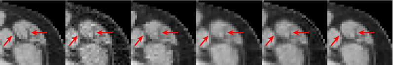
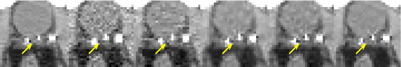
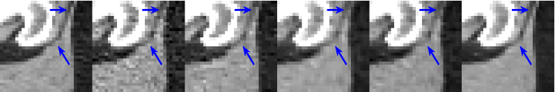
NDCT      FBP           TV     FBPConvNet PFBS-IR   PFBS-AIR

Figure 4: Zoom-in reconstruction results at dose level $I_{i}=5\times 10^{4}$. Three rows from up to bottom correspond to the red, yellow and blue boxes in Figure 3 respectively, with differences highlighted in arrows.

With further reduced dose, Fig. 5 and Fig. 7 show images reconstructed with dose level of $I_{i}=10^{4}$ and $I_{i}=5\times 10^{3}$, respectively. And the corresponding zoomed-in images are displayed in Fig. 6 and Fig. 8. These Figures suggest PFBS-AIR once again had the best reconstruction quality.

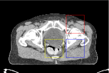
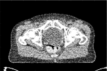
NDCT	FBP
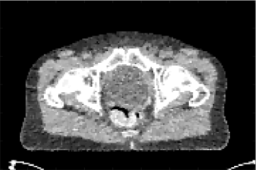
TV	FBPConvNet
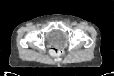
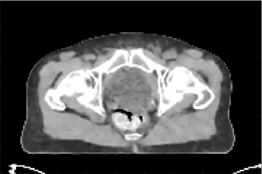
PFBS-IR	PFBS-AIR

Figure 5: Reconstruction results at dose level $I_{i}=10^{4}$.

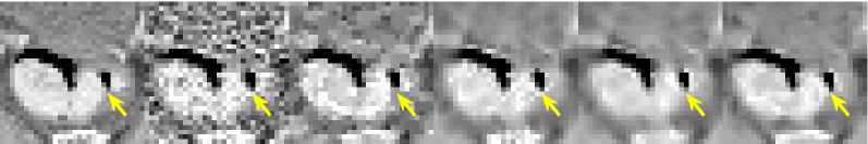
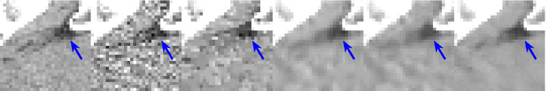
NDCT      FBP           TV     FBPConvNet PFBS-IR   PFBS-AIR

Figure 6: Zoom-in reconstruction results at dose level $I_{i}=10^{4}$. Three rows from up to bottom correspond to the red, yellow and blue boxes in Fig. 5 respectively, with differences highlighted in arrows.

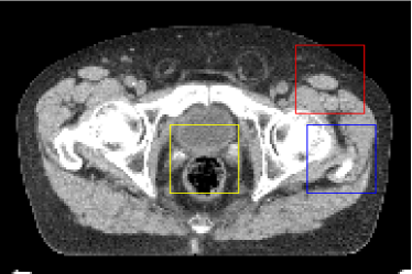
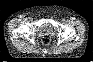
NDCT	FBP
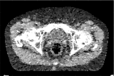
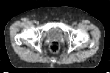
TV	FBPConvNet
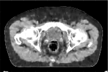
PFBS-IR	PFBS-AIR

Figure 7: Reconstruction results at dose level $I_{i}=5\times 10^{3}$.

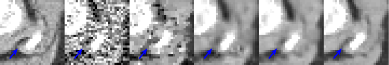
NDCT      FBP           TV     FBPConvNet PFBS-IR   PFBS-AIR

Figure 8: Zoom-in reconstruction results at dose level $I_{i}=5\times 10^{3}$. Three rows from up to bottom correspond to the red, yellow and blue boxes in Fig. 7 respectively, with differences highlighted in arrows.

On the other hand, the quantitative results corresponding to Fig. 3 , Fig. 5, and Fig. 7 are listed in Table II, Table III and Table IV respectively, which also shows the best performance if PFBS-AIR in terms of PSNR, RMSE, and SSIM.

TABLE II: Quantitative reconstruction results for the image slice in Fig. 3.

Dose level		FBP	TV	FBPConvNet	PFBS-IR	PFBS-AIR
$I_{i}=10^{5}$	PSNR	$42.4985$	$45.9763$	$47.8269$	$46.8933$	$\mathbb{51.5252}$
	RMSE	$~{}~{}0.0031$	$~{}~{}0.0021$	$~{}~{}0.0019$	$~{}~{}0.0021$	$~{}~{}\mathbb{0.0013}$
	SSIM	$~{}~{}0.9936$	$~{}~{}0.9972$	$~{}~{}0.9976$	$~{}~{}0.9974$	$~{}~{}\mathbb{0.9986}$
$I_{i}=5\times 10^{4}$	PSNR	$41.2469$	$44.4369$	$46.8502$	$45.0650$	$\mathbb{50.6984}$
	RMSE	$~{}~{}0.0036$	$~{}~{}0.0026$	$~{}~{}0.0021$	$~{}~{}0.0026$	$~{}~{}\mathbb{0.0014}$
	SSIM	$~{}~{}0.9904$	$~{}~{}0.9953$	$~{}~{}0.9966$	$~{}~{}0.9949$	$~{}~{}\mathbb{0.9984}$
$I_{i}=10^{4}$	PSNR	$36.3060$	$40.4774$	$43.8588$	$43.2313$	$\mathbb{45.3091}$
	RMSE	$~{}~{}0.0066$	$~{}~{}0.0041$	$~{}~{}0.0029$	$~{}~{}0.0031$	$~{}~{}\mathbb{0.0022}$
	SSIM	$~{}~{}0.9638$	$~{}~{}0.9874$	$~{}~{}0.9940$	$~{}~{}0.9921$	$~{}~{}\mathbb{0.9963}$
$I_{i}=5\times 10^{3}$	PSNR	$33.3903$	$38.8149$	$41.3073$	$42.5498$	$\mathbb{45.1596}$
	RMSE	$~{}~{}0.0094$	$~{}~{}0.0051$	$~{}~{}0.0036$	$~{}~{}0.0034$	$~{}~{}\mathbb{0.0027}$
	SSIM	$~{}~{}0.9280$	$~{}~{}0.9816$	$~{}~{}0.9912$	$~{}~{}0.9913$	$~{}~{}\mathbb{0.9944}$

TABLE III: Quantitative reconstruction results for the image slice in Fig. 5.

Dose level		FBP	TV	FBPConvNet	PFBS-IR	PFBS-AIR
$I_{i}=10^{5}$	PSNR	$39.0351$	$42.8197$	$44.7526$	$44.0438$	$\mathbb{48.1220}$
	RMSE	$~{}~{}0.0038$	$~{}~{}0.0025$	$~{}~{}0.0020$	$~{}~{}0.0022$	$~{}~{}\mathbb{0.0014}$
	SSIM	$~{}~{}0.9930$	$~{}~{}0.9832$	$~{}~{}0.9966$	$~{}~{}0.9970$	$~{}~{}\mathbb{0.9985}$
$I_{i}=5\times 10^{4}$	PSNR	$38.1533$	$41.6874$	$43.4913$	$41.3381$	$\mathbb{46.6175}$
	RMSE	$~{}~{}0.0042$	$~{}~{}0.0028$	$~{}~{}0.0023$	$~{}~{}0.0029$	$~{}~{}\mathbb{0.0016}$
	SSIM	$~{}~{}0.9903$	$~{}~{}0.9887$	$~{}~{}0.9960$	$~{}~{}0.9937$	$~{}~{}\mathbb{0.9980}$
$I_{i}=10^{4}$	PSNR	$34.6438$	$38.3544$	$40.7496$	$40.0446$	$\mathbb{43.0824}$
	RMSE	$~{}~{}0.0064$	$~{}~{}0.0042$	$~{}~{}0.0031$	$~{}~{}0.0034$	$~{}~{}\mathbb{0.0024}$
	SSIM	$~{}~{}0.9689$	$~{}~{}0.9954$	$~{}~{}0.9928$	$~{}~{}0.9911$	$~{}~{}\mathbb{0.9955}$
$I_{i}=5\times 10^{3}$	PSNR	$32.0027$	$36.0595$	$38.8226$	$39.2485$	$\mathbb{41.0346}$
	RMSE	$~{}~{}0.0087$	$~{}~{}0.0052$	$~{}~{}0.0038$	$~{}~{}0.0036$	$~{}~{}\mathbb{0.0029}$
	SSIM	$~{}~{}0.9415$	$~{}~{}0.9968$	$~{}~{}0.9899$	$~{}~{}0.9903$	$~{}~{}\mathbb{0.9937}$

TABLE IV: Quantitative results for the image slice in Fig. 7.

Dose level		FBP	TV	FBPConvNet	PFBS-IR	PFBS-AIR
$I_{i}=10^{5}$	PSNR	$39.1532$	$42.1400$	$43.4265$	$42.6736$	$\mathbb{46.3518}$
	RMSE	$~{}~{}0.0036$	$~{}~{}0.0025$	$~{}~{}0.0023$	$~{}~{}0.0025$	$~{}~{}\mathbb{0.0016}$
	SSIM	$~{}~{}0.9925$	$~{}~{}0.9961$	$~{}~{}0.9963$	$~{}~{}0.9961$	$~{}~{}\mathbb{0.9978}$
$I_{i}=5\times 10^{4}$	PSNR	$37.9938$	$40.7044$	$42.3560$	$40.6097$	$\mathbb{44.9094}$
	RMSE	$~{}~{}0.0041$	$~{}~{}0.0030$	$~{}~{}0.0025$	$~{}~{}0.0031$	$~{}~{}\mathbb{0.0019}$
	SSIM	$~{}~{}0.9889$	$~{}~{}0.9938$	$~{}~{}0.9949$	$~{}~{}0.9934$	$~{}~{}\mathbb{0.9970}$
$I_{i}=10^{4}$	PSNR	$33.4855$	$36.6776$	$39.7747$	$39.2662$	$\mathbb{41.4380}$
	RMSE	$~{}~{}0.0072$	$~{}~{}0.0048$	$~{}~{}0.0035$	$~{}~{}0.0037$	$~{}~{}\mathbb{0.0028}$
	SSIM	$~{}~{}0.9588$	$~{}~{}0.9839$	$~{}~{}0.9913$	$~{}~{}0.9896$	$~{}~{}\mathbb{0.9939}$
$I_{i}=5\times 10^{3}$	PSNR	$30.1080$	$35.0597$	$37.4600$	$37.7930$	$\mathbb{39.8136}$
	RMSE	$~{}0.0102$	$~{}~{}0.0058$	$~{}~{}0.0042$	$~{}~{}0.0041$	$~{}~{}\mathbb{0.0033}$
	SSIM	$~{}~{}0.9185$	$~{}~{}0.9763$	$~{}~{}0.9879$	$~{}~{}0.9880$	$~{}~{}\mathbb{0.9919}$

IV Conclusion

We have developed a DL-regularized image reconstruction method for LDCT, using the optimization framework of PFBS, with (A)IR for preconditioned data-fidelity update, namely PFBS-(A)IR. The preliminary results suggest PFBS-AIR had superior reconstruction quality over FBP (an AR method), TV (an IR method), FBPConvNet (a DL-based image postprocessing method), and PFBS-IR (a DL-regularized image reconstruction method), owing to the synergistic integration of AR, IR, and DL for LDCT.

References

- [1] X. Zhang and J. Froment, “Total variation based fourier reconstruction and regularization for computer tomography,” in Nuclear Science Symposium Conference Record, 2005 IEEE, vol. 4, pp. 2332–2336, IEEE, 2005.
- [2] E. Y. Sidky and X. Pan, “Image reconstruction in circular cone-beam computed tomography by constrained, total-variation minimization,” Physics in Medicine & Biology, vol. 53, no. 17, p. 4777, 2008.
- [3] G. Chen, J. Tang, and S. Leng, “Prior image constrained compressed sensing (PICCS): a method to accurately reconstruct dynamic CT images from highly undersampled projection data sets,” Medical physics, vol. 35, no. 2, pp. 660–663, 2008.
- [4] X. Jia, B. Dong, Y. Lou, and S. B. Jiang, “GPU-based iterative cone-beam CT reconstruction using tight frame regularization,” Physics in Medicine & Biology, vol. 56, no. 13, p. 3787, 2011.
- [5] H. Gao, R. Li, Y. Lin, and L. Xing, “4D cone beam CT via spatiotemporal tensor framelet,” Medical physics, vol. 39, no. 11, pp. 6943–6946, 2012.
- [6] X. Jia, Y. Lou, B. Dong, Z. Tian, and S. Jiang, “4D computed tomography reconstruction from few-projection data via temporal non-local regularization,” in International Conference on Medical Image Computing and Computer-Assisted Intervention, pp. 143–150, Springer, 2010.
- [7] H. Gao, J. Cai, Z. Shen, and H. Zhao, “Robust principal component analysis-based four-dimensional computed tomography,” Physics in Medicine & Biology, vol. 56, no. 11, p. 3181, 2011.
- [8] H. Gao, H. Yu, S. Osher, and G. Wang, “Multi-energy CT based on a prior rank, intensity and sparsity model (PRISM),” Inverse problems, vol. 27, no. 11, p. 115012, 2011.
- [9] J. Cai, X. Jia, H. Gao, S. B. Jiang, Z. Shen, and H. Zhao, “Cine cone beam CT reconstruction using low-rank matrix factorization: algorithm and a proof-of-principle study,” IEEE transactions on medical imaging, vol. 33, no. 8, pp. 1581–1591, 2014.
- [10] G. Chen and Y. Li, “Synchronized multiartifact reduction with tomographic reconstruction (SMART-RECON): A statistical model based iterative image reconstruction method to eliminate limited-view artifacts and to mitigate the temporal-average artifacts in time-resolved CT,” Medical physics, vol. 42, no. 8, pp. 4698–4707, 2015.
- [11] H. Gao, Y. Zhang, L. Ren, and F. Yin, “Principal component reconstruction (PCR) for cine CBCT with motion learning from 2D fluoroscopy,” Medical physics, vol. 45, no. 1, pp. 167–177, 2018.
- [12] H. Chen, Y. Zhang, M. K. Kalra, F. Lin, Y. Chen, P. Liao, J. Zhou, and G. Wang, “Low-dose CT with a residual encoder-decoder convolutional neural network,” IEEE transactions on medical imaging, vol. 36, no. 12, pp. 2524–2535, 2017.
- [13] Y. S. Han, J. Yoo, and J. C. Ye, “Deep residual learning for compressed sensing CT reconstruction via persistent homology analysis,” arXiv preprint arXiv:1611.06391, 2016.
- [14] H. Li and K. Mueller, “Low-dose CT streak artifacts removal using deep residual neural network,” in Proc. Fully Three-Dimensional Image Reconstruction Radiol. Nucl. Med.(Fully3D), pp. 191–194, 2017.
- [15] K. H. Jin, M. T. McCann, E. Froustey, and M. Unser, “Deep convolutional neural network for inverse problems in imaging,” IEEE Transactions on Image Processing, vol. 26, no. 9, pp. 4509–4522, 2017.
- [16] J. M. Wolterink, T. Leiner, M. A. Viergever, and I. Išgum, “Generative adversarial networks for noise reduction in low-dose CT,” IEEE transactions on medical imaging, vol. 36, no. 12, pp. 2536–2545, 2017.
- [17] Q. Yang, P. Yan, Y. Zhang, H. Yu, Y. Shi, X. Mou, M. K. Kalra, Y. Zhang, L. Sun, and G. Wang, “Low-dose CT image denoising using a generative adversarial network with wasserstein distance and perceptual loss,” IEEE transactions on medical imaging, vol. 37, no. 6, pp. 1348–1357, 2018.
- [18] E. Kang, J. Min, and J. C. Ye, “A deep convolutional neural network using directional wavelets for low-dose X-ray CT reconstruction,” Medical physics, vol. 44, no. 10, pp. e360–e375, 2017.
- [19] J. Gu and J. C. Ye, “Multi-scale wavelet domain residual learning for limited-angle CT reconstruction,” in Proc. Fully Three-Dimensional Image Reconstruction Radiol. Nucl. Med.(Fully3D), pp. 443–447, 2017.
- [20] J. Sun, H. Li, Z. Xu, et al., “Deep ADMM-Net for compressive sensing MRI,” in Advances in neural information processing systems, pp. 10–18, 2016.
- [21] M. Mardani, E. Gong, J. Y. Cheng, S. Vasanawala, G. Zaharchuk, M. Alley, N. Thakur, S. Han, W. Dally, J. M. Pauly, et al., “Deep generative adversarial networks for compressed sensing automates MRI,” arXiv preprint arXiv:1706.00051, 2017.
- [22] M. Mardani, H. Monajemi, V. Papyan, S. Vasanawala, D. Donoho, and J. Pauly, “Recurrent generative adversarial networks for proximal learning and automated compressive image recovery,” arXiv preprint arXiv:1711.10046, 2017.
- [23] H. Chen, Y. Zhang, Y. Chen, J. Zhang, W. Zhang, H. Sun, Y. Lv, P. Liao, J. Zhou, and G. Wang, “LEARN: Learned experts’ assessment-based reconstruction network for sparse-data CT,” IEEE transactions on medical imaging, vol. 37, no. 6, pp. 1333–1347, 2018.
- [24] J. Adler and O. Öktem, “Learned primal-dual reconstruction,” IEEE transactions on medical imaging, vol. 37, no. 6, pp. 1322–1332, 2018.
- [25] H. Gupta, K. H. Jin, H. Q. Nguyen, M. T. McCann, and M. Unser, “CNN-based projected gradient descent for consistent CT image reconstruction,” IEEE transactions on medical imaging, vol. 37, no. 6, pp. 1440–1453, 2018.
- [26] J. He, Y. Yang, Y. Wang, D. Zeng, Z. Bian, H. Zhang, J. Sun, Z. Xu, and J. Ma, “Optimizing a parameterized plug-and-play ADMM for iterative low-dose CT reconstruction,” IEEE transactions on medical imaging, vol. 38, no. 2, pp. 371–382, 2018.
- [27] H. Gao, “Fused analytical and iterative reconstruction (AIR) via modified proximal forward–backward splitting: a fdk-based iterative image reconstruction example for CBCT,” Physics in Medicine & Biology, vol. 61, no. 19, p. 7187, 2016.
- [28] P. L. Combettes and V. R. Wajs, “Signal recovery by proximal forward-backward splitting,” Multiscale Modeling & Simulation, vol. 4, no. 4, pp. 1168–1200, 2005.
- [29] J. Eckstein and D. P. Bertsekas, “On the douglas rachford splitting method and the proximal point algorithm for maximal monotone operators,” Mathematical Programming, vol. 55, no. 1-3, pp. 293–318, 1992.
- [30] R. Glowinski and P. Le Tallec, Augmented Lagrangian and operator-splitting methods in nonlinear mechanics, vol. 9. SIAM, 1989.
- [31] J. J. Moreau, “Fonctions convexes duales et points proximaux dans un espace hilbertien,” 1962.
- [32] X. Zhang, M. Burger, X. Bresson, and S. Osher, “Bregmanized nonlocal regularization for deconvolution and sparse reconstruction,” SIAM Journal on Imaging Sciences, vol. 3, no. 3, pp. 253–276, 2010.
- [33] G. Huang, Z. Liu, L. Van Der Maaten, and K. Q. Weinberger, “Densely connected convolutional networks,” in Proceedings of the IEEE conference on computer vision and pattern recognition, pp. 4700–4708, 2017.
- [34] Z. Zhang, X. Liang, X. Dong, Y. Xie, and G. Cao, “A sparse-view CT reconstruction method based on combination of DenseNet and deconvolution,” IEEE transactions on medical imaging, vol. 37, no. 6, pp. 1407–1417, 2018.
- [35] G. Chen, X. Hong, Q. Ding, Y. Zhang, H. Chen, S. Fu, Y. Zhao, X. Zhang, H. Ji, G. Wang, Q. Huang*, and H. Gao, “AirNet: Fused Analytical and Iterative Reconstruction with Densely Connected Deep Neural Networks for Sparse-Data CT,” Submitted.
- [36] A. Paszke, S. Gross, S. Chintala, G. Chanan, E. Yang, Z. DeVito, Z. Lin, A. Desmaison, L. Antiga, and A. Lerer, “Automatic differentiation in pytorch,” 2017.
- [37] Q. Ding, Y. Long, X. Zhang, and J. A. Fessler, “Statistical image reconstruction using mixed poisson-gaussian noise model for X-ray CT,” arXiv preprint arXiv:1801.09533, 2018.
- [38] Z. Wang, A. C. Bovik, H. R. Sheikh, E. P. Simoncelli, et al., “Image quality assessment: from error visibility to structural similarity,” IEEE transactions on image processing, vol. 13, no. 4, pp. 600–612, 2004.