Efficient estimation of a Gromov–Hausdorff distance between unweighted graphs

Abstract.

Gromov–Hausdorff distances measure shape difference between the objects representable as compact metric spaces, e.g. point clouds, manifolds, or graphs. Computing any Gromov–Hausdorff distance is equivalent to solving an NP-hard optimization problem, deeming the notion impractical for applications. In this paper we propose a polynomial algorithm for estimating the so-called modified Gromov–Hausdorff (mGH) distance, whose topological equivalence with the standard Gromov–Hausdorff (GH) distance was established in [Mém12] (Mémoli, F, Discrete & Computational Geometry, 48(2) 416-440, 2012). We implement the algorithm for the case of compact metric spaces induced by unweighted graphs as part of Python library scikit-tda, and demonstrate its performance on real-world and synthetic networks. The algorithm finds the mGH distances exactly on most graphs with the scale-free property. We use the computed mGH distances to successfully detect outliers in real-world social and computer networks.

List of notations

$\langle n\rangle$	index set $\{1,\ldots,n\}$, for $n\in\mathbb{N}$.
$\lceil a\rceil$	the ceiling of $a\in\mathbb{R}$: $\min\{n\in\mathbb{Z}:n\geq a\}$.
$\lfloor a\rceil$	the nearest integer to $a\in\mathbb{R}$.
$||\mathbf{v}||_{\infty}$	$l_{\infty}$-norm of vector $\mathbf{v}=\begin{bmatrix}v_{1}&v_{2}&\ldots&\end{bmatrix}$: $\max_{i}|v_{i}|$.
$\mathrm{row}_{i}(A)$	$i$-th row of matrix $A$: $\begin{bmatrix}A_{i,1}&A_{i,2}&\ldots&\end{bmatrix}$.
$A_{(i)(j)}$	matrix obtained from matrix $A$ by removing its $i$-th row and $j$-th column.
$d_{l^{\infty}}(A,B)$	$l_{\infty}$-induced matrix distance: $\max_{i,j}\left|A_{i,j}-B_{i,j}\right|$.
$|S|$	number of elements in set $S$.
$S^{\times n}$	Cartesian product $\underbrace{S\times\ldots\times S}_{n\text{ times}}$, for $n\in\mathbb{N}$.
$S\to T$	set of the mappings of $S$ into $T$.
$d_{\mathcal{H}}^{X}(S,T)$	the Hausdorff distance between the subsets $S,T$ of metric space $(X,d_{X})$:
	$\displaystyle d_{\mathcal{H}}^{X}(S,T)\buildrel\mathrm{def}\over{=}\max\left\{\sup_{s\in S}\inf_{t\in T}d_{X}(s,t),\;\sup_{t\in T}\inf_{s\in S}d_{X}(s,t)\right\}$.
$D^{X}$	distance matrix of metric space $(X,d_{X})$, where $X=\{x_{1},\ldots,x_{|X|}\}$:
	$D^{X}_{i,j}\buildrel\mathrm{def}\over{=}d_{X}(x_{i},x_{j})\quad\forall i,j=1,\ldots,|X|$.
$\mathcal{M}$	set of compact metric spaces.
$\operatorname{diam}X$	diameter of metric space $(X,d_{X})\in\mathcal{M}$: $\displaystyle\sup_{x,x^{\prime}\in X}d_{X}(x,x^{\prime})$.

1. Introduction

1.1. Isometry-invariant distances between metric spaces

The Gromov–Hausdorff (GH) distance, proposed by Gromov in [Gro81] ([Tuz16]), measures how far two compact metric spaces are from being isometric to each other. Since its conception four decades ago, the GH distance was mainly studied from a theoretical standpoint, as its computation poses an intractable combinatorial problem [CCSG⁺09, Mém07]. In particular, it was shown that, in the general case, even approximating the distance with a guarantee of a practical error bound cannot be done in polynomial time [Sch17]. In [MS04], the GH distance was first considered for shape comparison, and several of its computationally motivated relaxations were presented since then.

Different variations of the Gromov–Wasserstein distance, a relaxation of the GH distance for metric measure spaces motivated by the optimal transport problem [Vil03], were proposed in [Stu06] and in [Mém07], and further studied in e.g. [Mém09, Mém11, PCS16]. The Gromov–Wasserstein distances are based on a generalization of bijective assignments, which are less expressive than correspondences used in the GH distance. Similarly to the GH distance, computing the Gromov–Wasserstein distance also requires solving a non-convex optimization problem. Recently, semidefinite relaxations of both the GH and Gromov–Wasserstein distances were studied in [VBBW16]. While allowing polynomial-time approximation, these relaxations admit distance 0 between non-isometric objects, losing the desired property of being a metric. Another result of potential interest from [VBBW16] is a feasible algorithm for an upper bound of the GH (and therefore the mGH) distance. In [LD11], the authors define the conformal Wasserstein distance, inspired by the Gromov–Wasserstein distance. It is a metric on the isometry classes of Riemannian 2-manifolds that can be accurately approximated in polynomial time under some reasonable conditions.

In [Mém12], Mémoli introduces the modified Gromov–Hausdorff (mGH) distance, another relaxation of the GH distance that preserves the property of being a metric on the isometry classes of compact metric spaces. Same as the GH distance, the mGH distance is based on correspondences between the metric spaces, so that assigning additional counterparts from another metric space to a point does not take away from the strength of its previous assignments. It turns out that the two distances are topologically equivalent within precompact (in the GH-distance sense) families of compact metric spaces.

Although computing the mGH distance is of lower time complexity as compared to the standard GH distance, it similarly requires solving a hard optimization problem. Our focus on the mGH distance in this paper is partially motivated by the so-called ’structural theorem’ [Mém12], which allows for the decomposition of the computation into solving a sequence of polynomial-time problems.

1.2. Shape-based graph matching

Because graphs are ubiquitous in applications, the task of graph matching, i.e. measuring how much a pair of graphs are different from each other, is extensively studied. Common approaches to exact graph matching are those based on graph shape, such as subgraph isomorphism and maximum common subgraph [CFSV04, FPV14]. In fact, the maximum common subgraph problem is equivalent to a particular case of graph edit distance [Bun97], another ubiquitous concept in graph matching. The shape-based approaches appear in many fields including neuroscience [VWSD10], telecommunications [SKWB02], and chemoinformatics [RW02, VVGRM12]. While efficient heuristics for these approaches exist for special cases (e.g. planar graphs), applying them in the general case requires solving an NP-complete problem [Bun97, CFSV04].

Recently, the Gromov–Hausdorff framework for graph matching was explored both theoretically [ABK15] and in applications, e.g. in the fields of neuroscience [LCK⁺11, LCK⁺06, H⁺16], social sciences, and finance [H⁺16]. Undirected graphs admit metric space representation using the geodesic (shortest path length) distances on their vertex sets. However, the high computational cost of computing the isometry-invariant distances impedes a more widespread application of this approach.

1.3. Our contribution

Our main contribution is a theoretical framework for producing polynomial-time lower bounds of the GH distances. Furthermore, we present an algorithm for estimating the mGH distance, built upon this framework. We implement the algorithm for unweighted graphs, leveraging their properties to reduce polynomial order in the algorithm’s time complexity. While polynomial-time approximation of the GH distance was implemented for trees in [AFN⁺18], this is the first time a practical algorithm for a Gromov–Hausdorff distance is given for a broad class of graphs occurring in applications.

The rest of the paper is structured as follows. Section 2 briefly reviews [Mém13] to formally define the Gromov–Hausdorff distances, show their relation to each other, and state some of their properties. In Sections 3 and 4 we discuss the ideas for establishing lower and upper bounds, respectively, of the mGH distance between finite compact metric spaces. In Section 5, we describe the algorithm for estimating the mGH distance, show that it has polynomial time complexity, then discuss and present its implementation for the case of unweighted graphs. Computational examples from real-world and synthetic datasets are given in Section 6, while Section 7 summarizes our work. The Appendix contains pseudocode for the procedures and algorithms, omitted from the main paper for brevity.

2. Background

When talking about metric space given by set $X$ and distance function $d_{X}:X\times X\to\mathbb{R}$, we will use notation $(X,d_{X})$ and its shorter version $X$ interchangeably. We expect the distinction between a set $X$ and a metric space $X$ to be clear from the context.

2.1. Definition of the Gromov–Hausdorff distance

Given $(X,d_{X}),(Y,d_{Y})\in\mathcal{M}$, where $\mathcal{M}$ denotes the set of all compact metric spaces, the GH distance measures how far the two metric spaces are from being isometric. It considers any ”sufficiently rich” third metric space $(Z,d_{Z})$ that contains isometric copies of $X$ and $Y$, measuring the Hausdorff distance (in $Z$) between these copies, and minimizes over the choice of the isometric copies and $Z$. Formally, the GH distance is defined as

$$d_{\mathcal{GH}}(X,Y)\buildrel\mathrm{def}\over{=}\inf_{Z,\phi_{X},\phi_{Y}}d_{\mathcal{H}}^{Z}\big{(}\phi_{X}(X),\phi_{Y}(Y)\big{)},$$

where $\phi_{X}:X\to Z$ and $\phi_{Y}:Y\to Z$ are isometric embeddings of $X$ and $Y$ into $Z$, and $d_{\mathcal{H}}^{Z}$ is the Hausdorff distance in $Z$:

$$d_{\mathcal{H}}^{Z}(S,T)\buildrel\mathrm{def}\over{=}\max\Big{\{}\sup_{s\in S}\inf_{t\in T}d_{Z}(s,t),\sup_{t\in T}\inf_{s\in S}d_{Z}(s,t)\Big{\}}\quad\forall S,T\subseteq Z.$$

Gromov has shown in [Gro07] that $d_{\mathcal{GH}}$ is a metric on the isometry classes of $\mathcal{M}$, constituting what is called a Gromov–Hausdorff space.

Although the above definition gives the conceptual understanding of the GH distance, it is not very helpful from the computational standpoint. The next subsection introduces a more practical characterization of the GH distance.

2.2. Characterization of the GH distance

For two sets $X$ and $Y$, we say that relation $R\subseteq X\times Y$ is a correspondence if for every $x\in X$ there exists some $y\in Y$ s.t. $(x,y)\in R$ and for every $y\in Y$ there exists some $x\in X$ s.t. $(x,y)\in R$. We denote the set of all correspondences between $X$ and $Y$ by $\mathcal{R}(X,Y)$.

If $R$ is a relation between metric spaces $(X,d_{X})$ and $(Y,d_{Y})$, its distortion is defined as the number

$$\operatorname{dis}R\buildrel\mathrm{def}\over{=}\sup_{(x,y),(x^{\prime},y^{\prime})\in R}\big{|}d_{X}(x,x^{\prime})-d_{Y}(y,y^{\prime})\big{|}.$$

Note that any mapping $\varphi:X\to Y$ induces the relation $R_{\varphi}\buildrel\mathrm{def}\over{=}\big{\{}\big{(}x,\varphi(x)\big{)}:x\in X\big{\}}$, and we denote

$$\operatorname{dis}\varphi\buildrel\mathrm{def}\over{=}\operatorname{dis}R_{\varphi}=\sup_{x,x^{\prime}\in X}\big{|}d_{X}(x,x^{\prime})-d_{Y}\big{(}\varphi(x),\varphi(x^{\prime})\big{)}\big{|}.$$

Similarly, any $\psi:Y\to X$ induces the relation $R_{\psi}\buildrel\mathrm{def}\over{=}\big{\{}\big{(}\psi(y),y\big{)}:y\in Y\big{\}}$. If both $\varphi:X\to Y$ and $\psi:Y\to X$ are given, we can define the relation $R_{\varphi,\psi}\buildrel\mathrm{def}\over{=}R_{\varphi}\cup R_{\psi}$, and realize that it is actually a correspondence, $R_{\varphi,\psi}\in\mathcal{R}(X,Y)$.

A useful result in [KO99] identifies computing GH distance with solving an optimization problem, either over the correspondences between $X$ and $Y$ or over the functions $\varphi:X\to Y$ and $\psi:Y\to X$:

$$d_{\mathcal{GH}}(X,Y)=\frac{1}{2}\inf_{R\in\mathcal{R}(X,Y)}\operatorname{dis}R=\frac{1}{2}\inf_{\varphi,\psi}\operatorname{dis}R_{\varphi,\psi}.$$

Remark.

The first equality implies that computing $d_{\mathcal{GH}}(X,Y)$ for finite $X$ and $Y$ is equivalent to solving an instance of quadratic bottleneck assignment problem (QBAP), which is known to be NP-hard. Moreover, for any $\epsilon>0$, computing $\epsilon$-approximation of the optimal solution is also NP-hard. [BCPP98, PW⁺94].

By definition, distortion of any relation $R\subseteq X\times Y$ is bounded by $\operatorname{dis}R\leq d_{\max}$, where $d_{\max}\buildrel\mathrm{def}\over{=}\max\{\operatorname{diam}X,\operatorname{diam}Y\}$. Combined with the characterization of the GH distance, it implies that $d_{\mathcal{GH}}(X,Y)\leq\frac{1}{2}d_{\max}$.

Let $*$ denote the (compact) metric space that is comprised of exactly one point. For any correspondence $R\in\mathcal{R}(X,*)$, $\operatorname{dis}R=\sup_{x,x^{\prime}\in X}\big{|}d_{X}(x,x^{\prime})-0\big{|}=\operatorname{diam}X$. The above characterization yields $d_{\mathcal{GH}}(X,*)=\frac{1}{2}\operatorname{diam}X$, and, by the analogous argument, $d_{\mathcal{GH}}(Y,*)=\frac{1}{2}\operatorname{diam}Y$. From the triangle inequality for the GH distance, $d_{\mathcal{GH}}(X,Y)\geq\big{|}d_{\mathcal{GH}}(X,*)-d_{\mathcal{GH}}(Y,*)\big{|}=\frac{1}{2}|\operatorname{diam}X-\operatorname{diam}Y|$.

2.3. Modifying the GH distance

Recall that for some $\varphi:X\to Y$ and $\psi:Y\to X$, correspondence $R_{\varphi,\psi}$ is defined as $R_{\varphi,\psi}\buildrel\mathrm{def}\over{=}R_{\varphi}\cup R_{\psi}$. For any two elements in $R_{\varphi,\psi}$, either both belong to $R_{\varphi}$, or both belong to $R_{\psi}$, or one of them belongs to $R_{\varphi}$ while the other belongs to $R_{\psi}$. It follows that

$$\operatorname{dis}R_{\varphi,\psi}=\max\big{\{}\operatorname{dis}R_{\varphi},\operatorname{dis}R_{\psi},C_{\varphi,\psi}\big{\}},$$

where $C_{\varphi,\psi}\buildrel\mathrm{def}\over{=}\displaystyle\sup_{x\in X,y\in Y}\big{|}d_{X}\big{(}x,\psi(y)\big{)}-d_{Y}\big{(}\varphi(x),y\big{)}\big{|}$.

Note that the number $C_{\varphi,\psi}$ acts as a coupling term between the choices of $\varphi$ and $\psi$ in the optimization problem

$$d_{\mathcal{GH}}(X,Y)=\frac{1}{2}\inf_{\varphi,\psi}\max\big{\{}\operatorname{dis}R_{\varphi},\operatorname{dis}R_{\psi},C_{\varphi,\psi}\big{\}},$$

making its search space to be of the size $|X|^{|Y|}|Y|^{|X|}$. Discarding the coupling term $C_{\varphi,\psi}$ yields the notion of the modified Gromov–Hausdorff distance

$$\widehat{d}_{\mathcal{GH}}(X,Y)\buildrel\mathrm{def}\over{=}\frac{1}{2}\inf_{\varphi,\psi}\max\big{\{}\operatorname{dis}R_{\varphi},\operatorname{dis}R_{\psi}\big{\}}\leq d_{\mathcal{GH}}(X,Y).$$

Computing $\widehat{d}_{\mathcal{GH}}(X,Y)$ requires solving two decoupled optimization problems whose search spaces are of the size $|X|^{|Y|}$ and $|Y|^{|X|}$, respectively. An equivalent definition emphasizing this fact is given by

$$\widehat{d}_{\mathcal{GH}}(X,Y)\buildrel\mathrm{def}\over{=}\frac{1}{2}\max\big{\{}\inf_{\varphi}\operatorname{dis}R_{\varphi},\inf_{\psi}\operatorname{dis}R_{\psi}\big{\}}.$$

Similarly to $d_{\mathcal{GH}}$, $\widehat{d}_{\mathcal{GH}}$ is a metric on the isometry classes of $\mathcal{M}$. Moreover, $\widehat{d}_{\mathcal{GH}}$ is topologically equivalent to $d_{\mathcal{GH}}$ within GH-precompact families of metric spaces [Mém12].

2.4. Curvature sets and the structural theorem

Let $X\in\mathcal{M}$, and consider $(x_{1},\ldots,x_{n})\in X^{\times n}$, an $n$-tuple of points in $X$ for some $n\in\mathbb{N}$. The $n\times n$ matrix containing their pairwise distances is called the distance sample induced by $(x_{1},\ldots,x_{n})$, and denoted by $D^{(x_{1},\ldots,x_{n})}\buildrel\mathrm{def}\over{=}\big{(}d_{X}(x_{i},x_{j})\big{)}_{i,j=1}^{n}$. A distance sample generalizes the notion of distance matrix of $\{x_{1},\ldots,x_{n}\}$ when $x_{1},\ldots,x_{n}$ are not necessarily distinct. Unlike a distance matrix, a distance sample may contain zeros off the main diagonal.

The $n$-th curvature set of $X$ is then defined as a set of all $n\times n$ distance samples of $X$, denoted

$$\mathrm{\mathbf{K}}_{n}(X)\buildrel\mathrm{def}\over{=}\left\{D^{(x_{1},\ldots,x_{n})}:(x_{1},\ldots,x_{n})\in X^{\times n}\right\}.$$

For example, $\mathrm{\mathbf{K}}_{2}(X)$ contains the same information as the entries of $D^{X}$, the distance matrix of $X$; when $X$ is a smooth planar curve, then its curvature at every point can be calculated from the information contained in $\mathrm{\mathbf{K}}_{3}(X)$ [COS⁺98], thus providing motivation for the name curvature sets.

Curvature sets capture all the information about the shape of a compact metric space [Mém13]. In particular, any $X\in\mathcal{M}$ and $Y\in\mathcal{M}$ are isometric if and only if $\mathrm{\mathbf{K}}_{n}(X)=\mathrm{\mathbf{K}}_{n}(Y)$ for every $n\in\mathbb{N}$ [Gro07]. To discriminate the shapes of $X$ and $Y$, it is therefore reasonable to measure the difference between $\mathrm{\mathbf{K}}_{n}(X)$ and $\mathrm{\mathbf{K}}_{n}(Y)$ for various $n\in\mathbb{N}$. Since both $n$-th curvature sets are subsets of the same space $\mathbb{R}^{n\times n}$, Hausdorff distance is a natural metric between them. We equip the set of $n\times n$ matrices with distance $d_{l^{\infty}}(A,B)\buildrel\mathrm{def}\over{=}\max_{i,j}\left|A_{i,j}-B_{i,j}\right|$, and define

$$d_{\mathrm{\mathbf{K}}_{n}}(X,Y)\buildrel\mathrm{def}\over{=}\frac{1}{2}d_{\mathcal{H}}^{\mathbb{R}^{n\times n}}\big{(}\mathrm{\mathbf{K}}_{n}(X),\mathrm{\mathbf{K}}_{n}(Y)\big{)},$$

where $d_{\mathcal{H}}^{\mathbb{R}^{n\times n}}$ is the $d_{l^{\infty}}$-induced Hausdorff distance on $\mathbb{R}^{n\times n}$.

Remark.

The choice of distance $d_{l^{\infty}}:\mathbb{R}^{n\times n}\times\mathbb{R}^{n\times n}\to\mathbb{R}$ complies with the notion of distortion of a mapping. If $\varphi$ is a mapping from $X$ to $Y$ for $X=\{x_{1},\ldots,x_{|X|}\}$, $Y$ — metric spaces, then

$$\operatorname{dis}\varphi=d_{l^{\infty}}\left(D^{X},D^{\left(\varphi(x_{1}),\ldots,\varphi(x_{|X|})\right)}\right).$$

The fact that $\varphi$ can be non-injective provides intuition for the possibility of identical points in a tuple from the definition of a distance sample.

An important result, extensively relied upon in this paper, is the so-called ”structural theorem” for the mGH[Mém12, Mém13]:

$$\widehat{d}_{\mathcal{GH}}(X,Y)=\sup_{n\in\mathbb{N}}d_{\mathrm{\mathbf{K}}_{n}}(X,Y).$$

Note that the bounds of the GH distance from the inequalities $\frac{1}{2}|\operatorname{diam}X-\operatorname{diam}Y|\leq d_{\mathcal{GH}}(X,Y)\leq\frac{1}{2}d_{\max}$ also hold for the mGH distance:

$$\widehat{d}_{\mathcal{GH}}(X,Y) \geq d_{\mathrm{\mathbf{K}}_{2}}(X,Y)$$

$$=\frac{1}{2}d_{\mathcal{H}}^{\mathbb{R}}\Big{(}\big{\{}d_{X}(x,x^{\prime}):x,x^{\prime}\in X\big{\}},\big{\{}d_{Y}(y,y^{\prime}):y,y^{\prime}\in Y\big{\}}\Big{)}$$

$$\geq\frac{1}{2}\max\bigg{\{}\inf_{x,x^{\prime}\in X}\big{|}\operatorname{diam}Y-d_{X}(x,x^{\prime})\big{|},\inf_{y,y^{\prime}\in Y}\big{|}\operatorname{diam}X-d_{Y}(y,y^{\prime})\big{|}\bigg{\}}$$

$$=\frac{1}{2}\left|\operatorname{diam}X-\operatorname{diam}Y\right|,$$

while $\widehat{d}_{\mathcal{GH}}(X,Y)\leq d_{\mathcal{GH}}(X,Y)\leq d_{\max}$ trivially follows from the definition of the mGH distance.

3. Lower bound for $\widehat{d}_{\mathcal{GH}}(X,Y)$

This section provides theoretical results and algorithms for an informative lower bound for the mGH distance between a pair of metric spaces $X$ and $Y$. This and the following sections assume that the metric spaces are non-empty and finite, i.e. $1\leq|X|,|Y|<\infty$. When talking about algorithmic time complexities, we denote the input size with $N\buildrel\mathrm{def}\over{=}\max\{|X|,|Y|\}$.

Remark.

We note that efficient estimation of either of the GH distances between finite metric spaces allows for its estimation between infinite compact metric spaces with desired accuracy. This is because for any $X\in\mathcal{M}$ and $\epsilon>0$, there exist finite $X_{\epsilon}\subset X$ that is an $\epsilon$-net of $X$, and $\widehat{d}_{\mathcal{GH}}(X,X_{\epsilon})\leq d_{\mathcal{GH}}(X,X_{\epsilon})\leq d_{\mathcal{H}}(X,X_{\epsilon})\leq\epsilon$. Similarly, for any $Y\in\mathcal{M}$ there exists its finite $\epsilon$-net $Y_{\epsilon}$, and therefore

$$|d_{\mathcal{GH}}(X,Y)-d_{\mathcal{GH}}(X_{\epsilon},Y_{\epsilon})|\leq d_{\mathcal{GH}}(X,X_{\epsilon})+d_{\mathcal{GH}}(Y,Y_{\epsilon})\leq 2\epsilon.$$

Feasible algorithms for lower bounds are important in e.g. classification tasks, where knowledge that a distance exceeds some threshold can make computing the actual distance unnecessary. In particular, if the mGH distance between metric representations of two graphs is $>0$, it immediately follows that the graphs are not isomorphic.

3.1. $d$-bounded matrices

Let $A$ be a square matrix. We say that $A$ is $d$-bounded for some $d\in\mathbb{R}$ if every off-diagonal entry of $A$ is $\geq d$. Similarly, $A$ is positive-bounded if its off-diagonal entries are positive. Naturally, any $d$-bounded matrix for $d>0$ is also positive-bounded.

Note that a distance sample $D^{(x_{1},\ldots,x_{n})}$ of $X$ is $d$-bounded if and only if $d_{X}(x_{i},x_{j})\geq d\quad\forall i\neq j$, and positive-bounded if and only if $x_{1},\ldots,x_{n}$ are distinct. By non-negativity of a metric, any curvature is 0-bounded.

Claim 1.

Let $A$ and $B$ be square matrices of the same size. If $A$ is $d$-bounded for some $d>0$, and $B$ is 0-bounded but not positive-bounded, then $d_{l^{\infty}}(A,B)\geq d$.

Proof.

Since $B$ is not positive-bounded, $B_{i^{\prime},j^{\prime}}\leq 0$ for some $i^{\prime}\neq j^{\prime}$. From the 0-boundedness of $B$, $B_{i^{\prime},j^{\prime}}=0$, and therefore

$$d_{l^{\infty}}(A,B)\geq\left|A_{i^{\prime}j^{\prime}}-B_{i^{\prime}j^{\prime}}\right|\geq d.$$

∎

Recall that a matrix $B$ is a permutation similarity of a (same-sized) matrix $A$ if $B=PAP^{-1}$ for some permutation matrix $P$. Equivalently, $B$ is obtained from $A$ by permuting both its rows and its columns according to some permutation $\pi$: $B_{i,j}=A_{\pi(i),\pi(j)}$. Given $n\in\mathbb{N}$, we will denote the set of permutation similarities of $n\times n$ principal submatrices of $A$ by $\mathrm{PSPS}_{n}(A)$.

Claim 2.

A distance sample $K\in\mathrm{\mathbf{K}}_{n}(X)$ is positive-bounded if and only if it is a permutation similarity of a principal submatrix of $D^{X}$, i.e. if and only if $K\in\mathrm{PSPS}_{n}(D^{X})$. In particular, there are no positive-bounded curvatures in $\mathrm{\mathbf{K}}_{n}(X)$ if $n>|X|$.

Proof.

Recall that a distance sample is positive-bounded if and only if its underlying points are distinct. Since the points in $X$ are in one-to-one correspondence with the rows in $D^{X}$, the (permutations of the) tuples of distinct points in $X$ are in one-to-one correspondence with the (permutation similarities of the) principal submatrices of $D^{X}$. Since the size of a principal submatrix of $D^{X}$ is at most $|X|\times|X|$, there are no positive-bounded distance samples in $\mathrm{\mathbf{K}}_{n}(X)$ if $n>|X|$. ∎

Theorem A.

Let $K\in\mathrm{\mathbf{K}}_{n}(X)$ be $d$-bounded for some $d>0$. If $n>|Y|$, then $\widehat{d}_{\mathcal{GH}}(X,Y)\geq\frac{d}{2}$.

Proof.

Note that $L\in\mathrm{\mathbf{K}}_{n}(Y)$ implies that $L$ is 0-bounded (by non-negativity of a metric) and not positive-bounded (from Claim 2). Then

$$\widehat{d}_{\mathcal{GH}}(X,Y) \geq\frac{1}{2}d_{\mathcal{H}}^{\mathbb{R}^{n\times n}}\big{(}\mathrm{\mathbf{K}}_{n}(X),\mathrm{\mathbf{K}}_{n}(Y)\big{)}$$

$$\geq\frac{1}{2}\min_{L\in\mathrm{\mathbf{K}}_{n}(Y)}d_{l^{\infty}}(K,L)$$

$$\geq\frac{d}{2}.\hskip 113.81102pt\text{from Claim \ref{claim 1}}$$

∎

3.2. Obtaining $d$-bounded distance samples of large size

In order to apply Theorem A for some $d>0$, one needs to verify the existence of a $d$-bounded distance sample from $X$ that exceeds $Y$ in size. Ideally, one wants to know $M(X,d)$, the largest size of a $d$-bounded distance sample of $X$:

$$M(X,d)\buildrel\mathrm{def}\over{=}\max\big{\{}n\in\mathbb{N}:\text{$\exists$ $d$-bounded $K\in\mathrm{\mathbf{K}}_{n}(X)$}\big{\}}.$$

Equivalently, $M(X,d)$ is the so-called $d$-packing number of $X$: the largest number of points one can sample from $X$ such that they all are at least $d$ away from each other. Finding $M(X,d)$ is equivalent to finding the size of a maximum independent set of the graph $G=\big{(}X,\{(x_{i},x_{j}):d_{X}(x_{i},x_{j})<d\}\big{)}$. Unfortunately, this problem is known to be NP-hard [Kég02], and we therefore require approximation techniques to search for a sufficiently large $d$-bounded distance sample of $X$.

We implement greedy algorithm FindLarge$K$ (see Appendix A for the pseudocode) that, given the distance matrix of $X$ and some $d>0$, finds in $O(N^{3})$ time a $d$-bounded distance sample $K\in\mathrm{\mathbf{K}}_{\widetilde{M}(X,d)}(X)$, where $\widetilde{M}(X,d)$ is an approximation of $M(X,d)$. Informally, the algorithm iteratively removes rows (and same-index columns) from $D^{X}$ until all off-diagonal entries of the resulting curvature are $\geq d$. At each step, the algorithm chooses to remove a row with the largest (non-zero) number of off-diagonal entries $<d$, a so-called ”least $d$-bounded” row.

Note that $K$ needs not to be unique, since at any step there can be multiple ”least $d$-bounded” rows, those with the largest number of off-diagonal entries $<d$. Choosing which ”least $d$-bounded” row to remove allows to select for some desired characteristics in the retained rows of $K$. In particular, subsection 3.4 provides motivation to select for bigger entries in the resulting $d$-bounded curvature $K$. To accommodate this, we choose to remove at each step a ”least $d$-bounded” row with the smallest sum of off-diagonal entries $\geq d$, so-called ”smallest least $d$-bounded” row. Since uniqueness of a ”smallest least $d$-bounded” row is not guaranteed, we implemented procedure FindLeastBoundedRow (see Appendix B for the pseudocode) to find the index of the first such row in a matrix.

3.3. Using permutation similarities of principal submatrices of $D^{Y}$

Theorem A establishes $\widehat{d}_{\mathcal{GH}}(X,Y)\geq\frac{d}{2}$ from existence of some $d$-bounded distance sample of sufficiently large size. However, such distance samples might not exist in certain cases (e.g. when $|X|=|Y|$), thus deeming Theorem A inapplicable. The main result of this subsection, Theorem B, complements Theorem A by allowing verifying $\widehat{d}_{\mathcal{GH}}(X,Y)\geq\frac{d}{2}$ in those cases.

Lemma 1.

Let $K\in\mathrm{\mathbf{K}}_{n}(X)$ be $d$-bounded for some $d>0$, and let $n\leq|Y|$. If for some $i\in\langle n\rangle\buildrel\mathrm{def}\over{=}\{1,\ldots,n\}$

$$||\mathrm{row}_{i}(K)-\mathrm{row}_{i}(L)||_{\infty}\geq d\quad\forall L\in\mathrm{PSPS}_{n}(D^{Y}),$$

then $d_{l^{\infty}}\big{(}K,\mathrm{\mathbf{K}}_{n}(Y)\big{)}\geq d$.

Proof.

Let $L\in\mathrm{\mathbf{K}}_{n}(Y)$. If $L$ is not positive-bounded, $d_{l^{\infty}}(K,L)\geq d$ follows from Claim 1 and the fact that any distance sample is 0-bounded. If $L$ is positive-bounded, then $L\in\mathrm{PSPS}_{n}(D^{Y})$ from Claim 2, and the premise entails

$$d_{l^{\infty}}(K,L)\geq\big{|}\big{|}\mathrm{row}_{i}(K)-\mathrm{row}_{i}(L)\big{|}\big{|}_{\infty}\geq d.$$

Because $d_{l^{\infty}}(K,L)\geq d$ for an arbitrary choice of $L\in\mathrm{\mathbf{K}}_{n}(Y)$, we have $d_{l^{\infty}}\big{(}K,\mathrm{\mathbf{K}}_{n}(Y)\big{)}\geq d.$ ∎

Remark.

A naive approach to proving $d_{l^{\infty}}(K,\mathrm{\mathbf{K}}_{n}(Y))\geq d$ is to show that $d_{l^{\infty}}(K,L)\geq d$ for each $L\in\mathrm{\mathbf{K}}_{n}(Y)$, which comprises an instance of NP-hard quadratic bottleneck assignment problem [Mém13, BCPP98]. Instead, the premise of Lemma 1 (for a particular $i$) can be checked by solving at most $|Y|$ optimization problems of $O(|Y|)$ time complexity each, as will be shown in the next subsection.

Theorem B.

Let $K\in\mathrm{\mathbf{K}}_{n}(X)$ be $d$-bounded for some $d>0$, and let $n\leq|Y|$. If for some $i\in\langle n\rangle$

$$||\mathrm{row}_{i}(K)-\mathrm{row}_{i}(L)||_{\infty}\geq d\quad\forall L\in\mathrm{PSPS}_{n}(D^{Y}),$$

then $\widehat{d}_{\mathcal{GH}}(X,Y)\geq\frac{d}{2}$.

Proof.

$$\widehat{d}_{\mathcal{GH}}(X,Y) \geq\frac{1}{2}d_{\mathcal{H}}^{\mathbb{R}^{n\times n}}\big{(}\mathrm{\mathbf{K}}_{n}(X),\mathrm{\mathbf{K}}_{n}(Y)\big{)}$$

$$\geq\frac{1}{2}d_{l^{\infty}}\big{(}K,\mathrm{\mathbf{K}}_{n}(Y)\big{)}$$

$$\geq\frac{d}{2}.\hskip 113.81102pt\text{from Lemma \ref{lemma 1}}$$

∎

3.4. Verifying $\widehat{d}_{\mathcal{GH}}(X,Y)\geq\frac{d}{2}$

Let $d>0$. To see if we can verify $\widehat{d}_{\mathcal{GH}}(X,Y)\geq\frac{d}{2}$ from $D^{X}$ and $D^{Y}$, we start by calling FindLarge$K$ to obtain a $d$-bounded distance sample $K\in\mathrm{\mathbf{K}}_{n}(X)$, whose size $n$ is an approximation of $M(X,d)$. If $n>|Y|$, then $\widehat{d}_{\mathcal{GH}}(X,Y)\geq\frac{d}{2}$ follows immediately from Theorem A. If $n\leq|Y|$, we want to obtain this lower bound from Theorem B, which requires showing that some $i\in\langle n\rangle$ satisfies $||\mathrm{row}_{i}(K)-\mathrm{row}_{i}(L)||_{\infty}\geq d\quad\forall L\in\mathrm{PSPS}_{n}(D^{Y})$.

Let $i$ be fixed. If $L\in\mathrm{PSPS}_{n}(D^{Y})$, then all entries in $\mathrm{row}_{i}(L)$ come from one row of $D^{Y}$, with $L_{i,i}=0$ being the diagonal element in that row. The choice of $i$ thus induces a (disjoint) partition of $\mathrm{PSPS}_{n}(D^{Y})$:

$$\mathrm{PSPS}_{n}(D^{Y})=\bigcup_{j=1}^{|Y|}\mathrm{PSPS}^{n}_{i\leftarrow j}(D^{Y}),$$

where $\mathrm{PSPS}_{n}^{i\leftarrow j}(D^{Y})$ is the set of all permutation similarities of principal submatrices of $D^{Y}$ whose $i$-th row is comprised of the entries in $\mathrm{row}_{j}(D^{Y})$. Therefore, the condition $||\mathrm{row}_{i}(K)-\mathrm{row}_{i}(L)||_{\infty}\geq d\quad\forall L\in\mathrm{PSPS}_{n}(D^{Y})$ can be verified by showing that $||\mathrm{row}_{i}(K)-\mathrm{row}_{i}(L)||_{\infty}\geq d\quad\forall L\in\mathrm{PSPS}_{n}^{i\leftarrow j}(D^{Y})$ for every $j\in\langle|Y|\rangle$.

Let $j$, in addition to $i$, be fixed. Note that any $L\in\mathrm{PSPS}_{n}^{i\leftarrow j}(D^{Y})$ corresponds to an injective mapping $f_{L}:\langle n\rangle\to\langle|Y|\rangle$ that defines the entries from $\mathrm{row}_{j}(D^{Y})$ that populate $\mathrm{row}_{i}(L)$: $L_{i,k}=D^{Y}_{j,f_{L}(k)}$. In particular, $f_{L}(i)=j$, because $L_{i,i}=D^{Y}_{j,j}$ for any $L\in\mathrm{PSPS}_{n}^{i\leftarrow j}(D^{Y})$. Therefore, $||\mathrm{row}_{i}(K)-\mathrm{row}_{i}(L)||_{\infty}\geq d\quad\forall L\in\mathrm{PSPS}_{n}^{i\leftarrow j}(D^{Y})$ is equivalent to the non-existence of an injective $f_{L}:\langle n\rangle\to\langle|Y|\rangle$ such that $|K_{i,k}-D^{Y}_{j,f_{L}(k)}|<d\quad\forall k\in\langle n\rangle$ and $f_{L}(i)=j$. The decision about the existence of a feasible assignment $f_{L}$ between the entries of $\mathrm{row}_{i}(K)$ and $\mathrm{row}_{j}(D^{Y})$ is an instance of linear assignment feasibility problem. If such $f_{L}$ exists, it can be constructed by iteratively pairing the smallest unassigned $K_{i,k}$ to the smallest available $D^{Y}_{j,h}$ s.t. $|K_{i,k}-D^{Y}_{j,h}|<d$, that is, by setting $f_{L}(k)=h$. This way, if $D^{Y}_{j,h}$ is too small to satisfy $|K_{i,k}-D^{Y}_{j,h}|<d$ for $K_{i,k}$ (that is, if $D^{Y}_{j,h}\leq K_{i,k}-d$), then it is also too small for any other unassigned entries of $\mathrm{row}_{i}(K)$ and thus can be discarded. At the same time, if $K_{i,k}$ is too small to satisfy this inequality (that is, if $K_{i,k}\leq D^{Y}_{j,h}-d$), then it is also too small for any other available entries in $\mathrm{row}_{j}(D^{Y})$, implying that no feasible assignment $f_{L}$ exists and hence $||\mathrm{row}_{i}(K)-\mathrm{row}_{i}(L)||_{\infty}\geq d\quad\forall L\in\mathrm{PSPS}_{n}^{i\leftarrow j}(D^{Y})$. It follows that each entry in $\mathrm{row}_{j}(D^{Y})$ needs to be checked at most once, and hence solving the feasibility problem takes $O(|Y|)$ time if the entries in both $\mathrm{row}_{i}(K)$ and $\mathrm{row}_{j}(D^{Y})$ are sorted. Procedure SolveFeasibleAssignment (see Appendix C for the pseudocode) implements the solution for a pair of vectors, given their entries are arranged in ascending order. We note that ignoring the actual order of the (off-diagonal) entries in $\mathrm{row}_{i}(K)$ and $\mathrm{row}_{j}(D^{Y})$ reflects the fact that curvature sets are closed under permutations of the underlying tuples of points.

Remark.

Intuitively, either sufficiently small or sufficiently large entries in $\mathrm{row}_{i}(K)$ for some $i\in\langle n\rangle$ can make a feasible assignment $f_{L}$ impossible for every $j\in\langle|Y|\rangle$, yielding $||\mathrm{row}_{i}(K)-\mathrm{row}_{i}(L)||_{\infty}\geq d\quad\forall L\in\mathrm{PSPS}_{n}(D^{Y})$ and therefore $\widehat{d}_{\mathcal{GH}}(X,Y)\geq\frac{d}{2}$ from Theorem B. This provides the motivation behind considering the magnitude of the $\geq d$ entries when choosing a row to remove at each step of FindLarge$K$. Recall that such row is chosen by the auxiliary procedure FindLeastBoundedRow, that selects for bigger entries in the resulting $K$. The approach allows for a tighter lower bound in the case when the entries in $D^{X}$ are, generally speaking, bigger than those in $D^{Y}$. The converse case is then covered by similarly obtaining and handling a $d$-bounded distance sample of $Y$ (see the end of this subsection).

Calling SolveFeasibleAssignment$(\mathrm{row}_{i}(K),\mathrm{row}_{j}(D^{Y}),d)$ for every $j\in\langle|Y|\rangle$ is sufficient to check whether a particular $i$ satisfies $||\mathrm{row}_{i}(K)-\mathrm{row}_{i}(L)||_{\infty}\geq d\quad\forall L\in\mathrm{PSPS}_{n}(D^{Y})$. Procedure CheckTheoremB (see Appendix D for the pseudocode) makes such check for each $i\in\langle n\rangle$ to decide whether $\widehat{d}_{\mathcal{GH}}(X,Y)\geq\frac{d}{2}$ follows from Theorem B for the $d$-bounded $K$. The procedure sorts the entries in the rows of $K$ and $D^{Y}$ prior to the checks, which takes $O(N\log N)$ time for each of the $O(N)$ rows. This allows solving each of the $O(N^{2})$ feasibility problems in $O(N)$ time, making the time complexity of CheckTheoremB $O(N^{2}\log N+N^{3})=O(N^{3})$.

Note that both Theorem A and B regard a largest-size $d$-bounded distance sample of only one metric space, $X$. However, its counterpart for $Y$ is equally likely to provide information for discriminating the two metric spaces. Making use of the symmetry of $\widehat{d}_{\mathcal{GH}}$, we summarize theoretical findings of this section under $O(N^{3})$-time procedure VerifyLowerBound (see Appendix E for the pseudocode), that attempts to prove $\widehat{d}_{\mathcal{GH}}(X,Y)\geq\frac{d}{2}$.

3.5. Obtaining the lower bound

Procedure VerifyLowerBound is a decision algorithm that gives a ”yes” or ”no” answer to the question if a particular value can be proven to bound $\widehat{d}_{\mathcal{GH}}(X,Y)$ from below. In order to obtain an informative lower bound, one wants to find the largest value for which the answer is ”yes”. Since $\widehat{d}_{\mathcal{GH}}(X,Y)\leq\frac{1}{2}d_{\max}$, the answer must be ”no” for any value above $\frac{1}{2}d_{\max}$, and therefore it suffices to limit the scope to $(0,\frac{1}{2}d_{\max}]$. To avoid redundancy when checking the values from this interval, we consider the following result.

Claim 3.

Let $\Delta$ denote the set of absolute differences between the distances in $X$ and $Y$, $\Delta\buildrel\mathrm{def}\over{=}\{\left|d_{X}(x,x^{\prime})-d_{Y}(y,y^{\prime})\right|:x,x^{\prime}\in X,y,y^{\prime}\in Y\}$, and let $\{\delta_{i}\}_{i=1}^{|\Delta|}$ represent the sorting order of $\Delta$, $0=\delta_{1}<\ldots<\delta_{|\Delta|}=d_{\max}$. If $\delta_{i}<d_{1}<d_{2}\leq\delta_{i+1}$ for some $d_{1},d_{2}$ and $i\in\langle|\Delta|-1\rangle$, then $\textsc{VerifyLowerBound}(D^{X},D^{Y},d_{1})=\textsc{VerifyLowerBound}(D^{X},D^{Y},d_{2})$.

Proof.

VerifyLowerBound considers the value of its argument $d$ only through comparisons of the form ”$\delta<d$” for some $\delta$, that occur in FindLarge$K$ and SolveFeasibleAssignment. Note that the values of $\delta$ compared with $d$ in FindLarge$K$ are the entries of $D^{X}$ or $D^{Y}$, and therefore belong to $\Delta$ as $\{d_{X}(x,x^{\prime}):x,x^{\prime}\in X\},\{d_{Y}(y,y^{\prime}):y,y^{\prime}\in Y\}\subseteq\Delta$. The values of $\delta$ compared with $d$ in SolveFeasibleAssignment belong to $\Delta$ by construction.

For any $\delta\in\Delta$, $\delta<d_{1}$ if and only if $\delta<d_{2}$. This is because $\delta<d_{2}$ implies $\delta<d_{1}$ from $\delta\notin[d_{1},d_{2})$, while $\delta<d_{1}$ implies $\delta<d_{2}$ trivially. It follows that both FindLarge$K$ and SolveFeasibleAssignment yield identical outputs on $d_{1}$ and $d_{2}$ (and otherwise identical inputs), and hence so does VerifyLowerBound. ∎

Claim 3 implies that the largest $\delta\in\Delta$ s.t. $\textsc{VerifyLowerBound}(D^{X},D^{Y},\delta)=\mathrm{TRUE}$ is the largest $d\in\mathbb{R}$ s.t. $\textsc{VerifyLowerBound}(D^{X},D^{Y},d)=\mathrm{TRUE}$. We use this fact to implement the procedure FindLowerBound (see Appendix F for the pseudocode), that obtains a lower bound of $\widehat{d}_{\mathcal{GH}}(X,Y)$ by calling $\textsc{VerifyLowerBound}(D^{X},D^{Y},\delta)$ for each $\delta\in\Delta$ from largest to smallest, and stops once the output is TRUE. Since $|\Delta|=O(N^{4})$ in the general case, the time complexity of FindLowerBound is $O(N^{7})$.

Remark.

Using binary search on $\Delta$ instead of traversing its values in descending order reduces the number of calls to VerifyLowerBound from $O(N^{4})$ to $O(\log N)$, bringing the time complexity of FindLowerBound to $O(N^{3}\log N)$. We however note that, given some $d_{1}<d_{2}$, $\textsc{VerifyLowerBound}(D^{X},D^{Y},d_{2})=\mathrm{TRUE}$ does not guarantee $\textsc{VerifyLowerBound}(D^{X},D^{Y},d_{1})=\mathrm{TRUE}$, even though, trivially, $\widehat{d}_{\mathcal{GH}}(X,Y)\geq\frac{d_{2}}{2}>\frac{d_{1}}{2}$. It follows that relying on the binary search in FindLowerBound can result in failing to find the largest $\delta\in\Delta$ s.t. $\textsc{VerifyLowerBound}(D^{X},D^{Y},\delta)=\mathrm{TRUE}$, and thus in reducing time complexity at the cost of lower accuracy.

4. Upper bound for $\widehat{d}_{\mathcal{GH}}(X,Y)$

To obtain an upper bound of $\widehat{d}_{\mathcal{GH}}(X,Y)$, we recall the definition

$$\widehat{d}_{\mathcal{GH}}(X,Y)\buildrel\mathrm{def}\over{=}\frac{1}{2}\max\{\inf_{\varphi}\operatorname{dis}\varphi,\inf_{\psi}\operatorname{dis}\psi\},$$

where $\varphi$ and $\psi$ are the mappings $\varphi:X\to Y$ and $\psi:Y\to X$ and the infimums are taken over the corresponding function spaces. It follows that $\widehat{d}_{\mathcal{GH}}(X,Y)\leq\frac{1}{2}\max\{\operatorname{dis}\varphi,\operatorname{dis}\psi\}$ for any particular choice of $\varphi$ and $\psi$. Considering the exponential size of function spaces, we rely on a small randomized sample of mappings to tighten the upper bound. To sample $\varphi:X\to Y$, we use the construction method, a heuristic for solving quadratic assignment problems [Gil62, BCPP98]. The construction method iteratively maps each $x\in X$ to some $y\in Y$, chosen by a greedy algorithm to minimize $\operatorname{dis}\varphi$ as described below.

Let $X=\{x_{1},\ldots,x_{|X|}\}$ and $Y=\{y_{1},\ldots,y_{|Y|}\}$. We randomly choose a permutation $\pi$ of $\langle|X|\rangle$ to represent the order in which the points in $X$ are mapped. At step $i$ we map $x_{\pi(i)}$ by choosing $y_{j_{i}}$ and setting $\varphi(x_{\pi(i)})\buildrel\mathrm{def}\over{=}y_{j_{i}}$. We represent these choices by inductive construction $R_{\varphi}^{(i)}=R_{\varphi}^{(i-1)}\cup\{(x_{\pi(i)},y_{j_{i}})\}$ for $i=1,\ldots,|X|$, where $R_{\varphi}^{(0)}\buildrel\mathrm{def}\over{=}\emptyset$. The particular choice of $y_{j_{i}}$ at step $i$ is made to minimize distortion of resultant $R_{\varphi}^{(i)}$:

$$y_{j_{i}}\in\operatorname*{arg\,min}_{y\in Y}\,\operatorname{dis}\Big{(}R_{\varphi}^{(i-1)}\cup\big{\{}(x_{\pi(i)},y)\big{\}}\Big{)}.$$

After carrying out all $|X|$ steps, $\varphi:X\to Y$ is given by the constructed relation $R_{\varphi}\buildrel\mathrm{def}\over{=}R_{\varphi}^{(|X|)}$, and by definition, $\operatorname{dis}\varphi=\operatorname{dis}R_{\varphi}$.

Notice the possible ambiguity in the choice of $y_{j_{i}}$ when $y\in Y$ minimizing $\operatorname{dis}\Big{(}R_{\varphi}^{(i-1)}\cup\big{\{}(x_{\pi(i)},y)\big{\}}\Big{)}$ is not unique. In particular, any $y\in Y$ can be chosen as $y_{j_{1}}$ at step 1, since $\operatorname{dis}\big{\{}(x_{\pi(i)},y_{j_{1}})\big{\}}=0$ is invariant to the said choice. In the case of such ambiguity, our implementation simply decides to map $x_{\pi(i)}$ to $y_{j_{i}}$ of the smallest index $j_{i}$. However, in applications one might want to modify this logic to leverage the knowledge of the relationship between the points from two metric spaces.

We formalize the above heuristic under a randomized, $O(N^{3})$-time procedure SampleSmallDistortion (see Appendix G for the pseudocode) that samples a mapping between the two metric spaces with the intent of minimizing its distortion, and outputs this distortion. We then describe an algorithm FindUpperBound (see Appendix H for the pseudocode), that repeatedly calls SampleSmallDistortion to find $\varphi^{*}:X\to Y$ and $\psi^{*}:Y\to X$, the mappings of the smallest distortion among those sampled from $X\to Y$ and $Y\to X$, respectively, and finds an upper bound for $\widehat{d}_{\mathcal{GH}}(X,Y)$ as $\frac{1}{2}\max\{\operatorname{dis}\varphi^{*},\operatorname{dis}\psi^{*}\}$. The time complexity of FindUpperBound is therefore $O(sN^{3})$, where $s$ is the total number of sampled mappings.

5. Algorithm for estimating $\widehat{d}_{\mathcal{GH}}(X,Y)$

The algorithm for estimating the mGH distance between compact metric spaces $X$ and $Y$ (”the algorithm”) consists of the calls $\textsc{FindLowerBound}(D^{X},D^{Y})$ and $\textsc{FindUpperBound}(D^{X},D^{Y})$. Note that $\widehat{d}_{\mathcal{GH}}(X,Y)$ is found exactly whenever the outputs of the two procedures match. Time complexity of the algorithm is $O(N^{7})$ whenever the number of mappings sampled from $X\to Y$ and $Y\to X$ in FindUpperBound is constrained to $s=O(N^{4})$.

To obtain a more practical result, we now consider a special case of metric spaces induced by unweighted undirected graphs. We show that estimating the mGH distance between such metric spaces in many applications has time complexity $O(N^{3}\log N)$, and present our implementation of the algorithm in Python.

5.1. $\widehat{d}_{\mathcal{GH}}$ between unweighted undirected graphs

Let $G=(V_{G},E_{G})$ be a finite undirected graph. For every pair of vertices $v,v^{\prime}\in V_{G}$, we define $d_{G}(v,v^{\prime})$ as the shortest path length between $v$ to $v^{\prime}$. If weights of the edges in $E_{G}$ are positive, the resulting function $d_{G}:V_{G}\times V_{G}\to[0,\infty]$ is a metric on $V_{G}$. We say that the metric space $(V_{G},d_{G})$ is induced by graph $G$, and note that its size $|V_{G}|$ is the order of $G$. By convention, the shortest path length between vertices from different connected components of a graph is defined as $\infty$, and therefore $(V_{G},d_{G})$ is compact if and only if graph $G$ is connected.

For brevity, we will use notation $G\buildrel\mathrm{def}\over{=}(V_{G},d_{G})$, assuming that the distinction between graph $G$ and metric space $G$ induced by this graph is clear from the context. In particular, we refer to the mGH distance between compact metric spaces induced by undirected connected graphs $G$ and $H$ as $\widehat{d}_{\mathcal{GH}}(G,H)$, or even call it ”the mGH distance between graphs $G$ and $H$”.

Let $G,H$ be unweighted undirected connected graphs. Note that $\widehat{d}_{\mathcal{GH}}(G,H)=0$ if and only if graphs $G$ and $H$ are isomorphic. We use the following result to reduce the computational cost of estimating $\widehat{d}_{\mathcal{GH}}(G,H)$ as compared to that in the general case.

Claim 4.

If $G$ is unweighted undirected connected graph, all entries in distance matrix $D^{G}$ of the corresponding compact metric space are from $\{0,1,\ldots,\operatorname{diam}G\}$.

Proof.

Any path in an unweighted connected graph is of non-negative integer length that, by definition, does not exceed the diameter of the graph. ∎

Claim 4 implies that there are at most $d_{\max}+1$ distinct entries in any distance sample of either $G$ or $H$, where $d_{\max}\buildrel\mathrm{def}\over{=}\max\{\operatorname{diam}G,\operatorname{diam}H\}$. Recall that the procedure SolveFeasibleAssignment requires the entries in its input vectors to be sorted, which allows representing each of the two vectors as a frequency distribution of the values $0,1,\ldots,d_{\max}$. Such grouping of identical entries allows the procedure to make bulk assignments when constructing the optimal solution as described in subsection 3.4. Assigning identical entries in bulk reduces the time complexity of SolveFeasibleAssignment from $O(N)$ to $O(d_{\max})$ and makes the complexity of CheckTheoremB $O(N^{2}d_{\max})$, where $N\buildrel\mathrm{def}\over{=}\max\{|V_{G}|,|V_{H}|\}$.

Remark.

From the perspective of optimization theory, representing vectors as frequency distributions of their entries reformulates the linear assignment feasibility problem of SolveFeasibleAssignment as a transportation feasibility problem.

Another implication of Claim 4 narrows the set of absolute differences between the distances in $G$ and $H$ to $\Delta=\{0,1,\ldots,d_{\max}\}$, reducing the time complexity of traversing its elements from $O(N^{4})$ to $O(d_{\max})$. This bounds the time complexity of FindLowerBound by $O(N^{3}d_{\max})$. The complexity of the entire algorithm is therefore $O(N^{3}d_{\max})$ when the number of sampled mappings is $s=O(d_{\max})$.

Network diameter often scales logarithmically with network size, e.g. in Erdős–Rényi random graph model [AB02] and Watts–Strogatz small-world model [WS98], or even sublogarithmically, e.g. in the configuration model with i.i.d. degrees [HHZ07] and Barabási–Albert preferential attachment model [CH03]. This suggests the time complexity of the algorithm in applications to be $O(N^{3}\log N)$, deeming it practical for shape comparison for graphs of up to a moderate order.

5.2. Implementation

We have implemented the algorithm for estimating mGH between unweighted graphs in Python 3.7 as part of scikit-tda package [ST19] (https://github.com/scikit-tda). Our implementation takes adjacency matrices (optionally in sparse format) of unweighted undirected graphs as inputs. If an adjacency matrix corresponds to a disconnected graph, the algorithm approximates it with its largest connected component. The number of mappings to sample from $X\to Y$ and $Y\to X$ in FindUpperBound is parametrized as a function of $|X|$ and $|Y|$.

6. Computational examples

This section demonstrates the performance of the algorithm on some real-world and synthetic networks. The real-world networks were sourced from the Enron email corpus [KY04], the cybersecurity dataset collected at Los Alamos National Laboratory [Ken16], and the functional magnetic resonance imaging dataset ABIDE I [DMYL⁺14].

6.1. Methodology and tools

To estimate mGH distances between the graphs, we use our implementation of the algorithm from subsection 5.2. We set the number of mappings from $X\to Y$ and $Y\to X$ to sample by the procedure FindUpperBound to $\lceil\sqrt{|X|}\log(|X|+1)\rceil$ and $\lceil\sqrt{|Y|}\log(|Y|+1)\rceil$, respectively.

Given a pair of connected graphs, we approximate the mGH distance between them by $\tilde{d}\buildrel\mathrm{def}\over{=}\frac{b_{L}+b_{U}}{2}$, where $b_{L}$ and $b_{U}$ are the lower and upper bounds produced by the algorithm. The relative error of the algorithm is estimated by

$$\eta\buildrel\mathrm{def}\over{=}\begin{cases}\frac{b_{U}-b_{L}}{2\tilde{d}}=\frac{b_{U}-b_{L}}{b_{L}+b_{U}},&\text{if $b_{U}>0$}\\ 0,&\text{if $b_{U}=0$}\end{cases},$$

noting that the case of $b_{U}=0$ implies that the algorithm has found the mGH distance of 0 exactly. In addition, we compute the utility coefficient defined by

$$\upsilon\buildrel\mathrm{def}\over{=}\begin{cases}\frac{b_{L}-b^{\prime}_{L}}{2\tilde{d}}=\frac{b_{L}-b^{\prime}_{L}}{b_{L}+b_{U}},&\text{if $b_{U}>0$}\\ 0,&\text{if $b_{U}=0$}\end{cases},$$

where $b^{\prime}_{L}\leq b_{L}$ is the baseline lower bound: $b^{\prime}_{L}\buildrel\mathrm{def}\over{=}\frac{1}{2}|\operatorname{diam}X-\operatorname{diam}Y|\leq\widehat{d}_{\mathcal{GH}}(X,Y)$ for $X,Y\in\mathcal{M}$. The utility coefficient thus quantifies the tightening of the lower bound achieved by using Theorems A and B.

Due to the possible suboptimality of the mappings selected by using the construction method (see section 4), the upper bound may not be computed accurately enough. From the definition of relative error $\eta$ and utility coefficient $\upsilon$, a sufficiently loose upper bound can make $\eta$ arbitrarily close to 1 and $\upsilon$ — arbitrarily small.

We measured $\eta$ and $\upsilon$ separately for each dataset. For the real-world data, we also used the approximated distances $\tilde{d}$ to identify graphs of outlying shapes and matched these graphs to events or features of importance in application domains, following the approach taken in e.g. [BK04, BDH⁺06, KVF13, Pin05]. Unlike [BK04, KVF13], and [Pin05] that focus on local time outliers (under the assumption of similarity between graphs from consecutive time steps), we considered the outliers with respect to the entire time range (where applicable), similarly to [BDH⁺06].

To identify the outliers, we applied the Local Outlier Probability (LoOP) method [KKSZ09] to the graphs using their approximated pairwise mGH distances. LoOP uses a local space approach to outlier detection and is robust with respect to the choice of parameters [KKSZ09]. The score assigned by LoOP to a data object is interpreted as the probability of the object to be an outlier. We binarize the score into outlier/non-outlier classification using the commonly accepted confidence levels of 95%, 99%, and 99.9% as thresholds, chosen empirically for each individual dataset. We used the implementation of LoOP in Python [Con18] (version 0.2.1), modified by us to allow non-Euclidean distances between the objects. We ran LoOP with locality and significance parameters set to $k=20$ and $\lambda=1$, respectively.

The synthetic graphs were generated according to Erdős–Rényi, Watts–Strogatz, and Barabási–Albert network models. We used implementations of the models provided in [HSSC08] (version 2.1).

All computations were performed on a single 2.70GHz core of Intel i7-7500U CPU.

6.2. Enron email corpus

Enron email corpus (available at https://www.cs.cmu.edu/~./enron/) represents a collection of email conversations between the employees, mostly senior management, of the Enron corporation from October 1998 to March 2002. We used the latest version of the dataset from May 7, 2015, which contains roughly 500K emails from 150 employees.

Associating employees with graph vertices, we view the dataset as a dynamic network whose 174 instances reflect weekly corporate email exchange over the course of 3.5 years. An (unweighted) edge connecting a pair of vertices in a network instance means a mutual exchange of at least one email between the two employees on a particular week. The time resolution of 1 week was suggested in [SBWG10] for providing an appropriate balance between noise reduction and information loss in Enron dataset.

We expected major events related to the Enron scandal in the end of 2001 to cause abnormal patterns of weekly email exchange between the senior management, distorting the shape of the corresponding network instances. As a consequence, metric spaces generated by such network instances would be anomalously far from the rest with respect to the mGH distance.

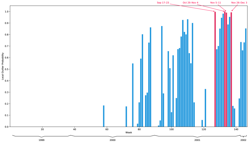
Figure 1. Outlier probabilities assigned to the weekly email exchange networks. Red indicates outlier probabilities $>0.99$, corresponding to the weeks of Sep 17, Oct 29, Nov 5, and Nov 26 in the year 2001.

In preparation for the analysis, we discarded all empty network instances corresponding to the weeks of no email exchange between the employees (of which all 28 weeks happened before May 1999). Each of the remaining 146 graphs was then replaced with its largest connected component. The distribution of the order of the resulting graphs had a mean of 68.2, a standard deviation of 99.8, and a maximum of 706.

We estimated the mGH distances in all 10,585 distinct pairs of the non-empty connected network instances. Average graph order and computing time per one pair were distributed as $68.2\pm 70.3$ and $0.93\mathrm{s}\pm 3.91\mathrm{s}$, respectively (where $\mu\pm\sigma$ refers to distribution with a mean of $\mu$ and a standard deviation of $\sigma$; no assumptions of normality are made, and we use standard deviation solely as a measure of spread). The algorithm found exact mGH distances in 74.4% of the graph pairs, with relative error $\eta$ and utility coefficient $\upsilon$ distributed as $0.057\pm 0.118$ and $0.043\pm 0.085$, respectively. The ratio between the means of $\upsilon$ and $\eta$ implies that using Theorems A and B on average reduced the relative error by a factor of 1.75.

We ran LoOP on the network instances using their (approximated) pairwise mGH distances $\tilde{d}$. The resulting outlier probability assigned to each network instance (Figure 1) thus measures the abnormality of its shape.

To see if the abnormal shape of email exchange corresponds to events of high importance from the Enron timeline, we applied the threshold of 0.99 to the outlier probabilities. Three out of four network instances that scored above the threshold correspond to the weeks of known important events in 2001, namely the weeks of Oct 29, Nov 5, and Nov 26 (each date is a Monday). As the closing stock price of Enron hit an all-time low on Friday, Oct 26, Enron’s chairman and CEO Kenneth Lay was making multiple calls for help to Treasure Secretary Paul O’Neill and Commerce Secretary Donald Evans on Oct 28–29. Enron fired both its treasurer and in-house attorney on Nov 5, admitted to overstating its profits for the last five years by $600M on Nov 8, and agreed to be acquired by Dynegy Inc. for $9B on Nov 9. On Nov 28, Dynegy Inc. aborted the plan to buy Enron, and on Dec 2, Enron went bankrupt.

We conclude that the abnormal shape of email exchange networks tends to correspond to disturbances in their environment, and that the algorithm estimates the mGH distance accurately enough to capture it.

6.3. LANL cybersecurity dataset

Los Alamos National Laboratory (LANL) cybersecurity dataset (available at https://csr.lanl.gov/data/cyber1/) represents 58 consecutive days of event data collected from LANL’s corporate computer network [Ken16]. For our purposes, we considered its part containing records of authentication events, generated by roughly 11K users on 18K computers, and collected from individual Windows-based desktops and servers. During the 58-day data collection period, a “red team” penetration testing operation had taken place. As a consequence, a small subset of authentications were labeled as red team compromise events, presenting well-defined bad behavior that differed from normal user and computer activity. The labeling is not guaranteed to be exhaustive, and authentication events corresponding to red team actions, but not labeled as such, are likely to be present in the data. [HRD16]

Each authentication event occurs between a pair of source and destination computers. Viewing the computers as graph vertices, we associated each user with a dynamic network, whose instances reflect their daily authentication activity within the 58-day period. An (unweighted) edge connecting a pair of vertices in a network instance means that at least one authentication event by the user has occurred between the two computers on a particular day. The user-based approach to graph representation of the data aims to capture the patterns of user account misuse that are expected to occur during a cyberattack.

Our objective was to develop an unsupervised approach that can identify the red team activity associated with a user’s account. We expected that frequent compromise events within the course of one day should distort the shape of the corresponding network instance. As a consequence, metric spaces generated by such network instances would be anomalously far from the rest.

For the analysis, we selected 20 users with the highest total of associated red team events and randomly chose another 20 users from those unaffected by the red team activity (see Figure 2). Each of their 40 dynamic networks initially comprised of 58 instances. We discarded all empty network instances corresponding to the days of inactivity of a user account, and replaced each of the remaining 1,997 graphs with its largest connected component. The distribution of the order in the resulting graphs had a mean of 32.7 and a standard deviation of 75.8. The largest graphs were associated with the red team-affected user U1653@DOM1 — their order was distributed with a mean of 178.2, a standard deviation of 391.5, and a maximum of 2,343.

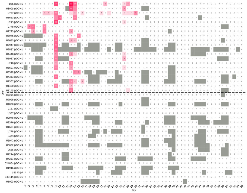
Figure 2. Frequency of red team events in daily authentication activity of the selected users. Grey indicates days of no authentication activity by user. Dashed line separates the two groups of 20 users.

Separately for each of the selected users, we estimated the mGH distances in all distinct pairs of the non-empty connected network instances associated with her account. Table 1 shows average graph order in a pair and the performance metrics of the algorithm, aggregated per user subsets. We note that using Theorems A and B has reduced the relative error by a factor of 3.5 on average. In addition, the algorithm did not seem to perform worse on the larger graphs associated with user U1653@DOM1.

	# of	average	computing	exact	relative	utility
	pairs	graph order	time	distances	error $\eta$	coefficient $\upsilon$
all 40 users	50316	$34.2\pm 60.7$	$0.44\mathrm{s}\pm 14.09\mathrm{s}$	84.7%	$0.049\pm 0.121$	$0.121\pm 0.127$
U1653@DOM1	1540	$178.2\pm 274.3$	$13.52\mathrm{s}\pm 79.46\mathrm{s}$	94.2%	$0.012\pm 0.051$	$0.135\pm 0.123$
other 39 users	48776	$29.7\pm 27.3$	$0.028\mathrm{s}\pm 0.058\mathrm{s}$	84.4%	$0.051\pm 0.122$	$0.120\pm 0.127$

Table 1. Performance of the algorithm on user-based daily authentication graphs. $\mu\pm\sigma$ denotes that the distribution of a variable across the graph pairs has a mean of $\mu$ and a standard deviation of $\sigma$.

Figure 3. Outlier probability assigned to user-based daily authentication graphs. Red indicates outlier probabilities $>0.999$. Grey indicates empty graphs (excluded from analysis). The dashed line separates the two groups of 20 users.

Separately for each user, we ran LoOP on the associated network instances using their (approximated) pairwise mGH distances $\tilde{d}$. The resulting outlier probability assigned to each network instance (Figure 3) thus measures the abnormality of its shape for the particular user.

To see if the days of high compromise activity can be identified from the abnormal shape of the corresponding network instances, we approached the identification as a binary classification task. User’s daily activity is considered a compromise if it includes at least 30 red team events, and is predicted as such if the outlier probability assigned to the corresponding network instance is $>0.999$. The resulting confusion matrix of our shape-based binary classifier is shown in Table 2, establishing its accuracy, precision, and recall as 99.5%, 18.2%, and 100%, respectively.

		predicted
		compromise	not compromise	total
actual	compromise	2	0	2
	not compromise	9	1986	1995
	total	11	1986	1997

Table 2. Confusion matrix of the shape-based binary classifier.

Even though recall is prioritized over precision when identifying intrusions, low precision can be impractical when using the classifier alone. However, high recall suggests that combining the shape-based classifier with another method can improve performance of the latter. For example, classifying daily activity as a compromise if and only if both methods agree on it is likely to increase the other method’s precision without sacrificing its recall.

We conclude that sufficiently frequent compromise behavior tends to distort the shape of networks representing user authentication activity, and that the algorithm estimates the mGH distance accurately enough to pick up the distortion.

6.4. ABIDE I dataset

The Autism Brain Imaging Data Exchange I (ABIDE I, http://fcon_1000.projects.nitrc.org/indi/abide/abide_I.html) [DMYL⁺14] is a resting state functional magnetic resonance imaging dataset, collected to improve understanding of the neural bases of autism. Besides the diagnostic group (autism or healthy control), the information collected from the study subjects also includes their sex, age, handedness category, IQ, and current medication status. We considered the preprocessed version of ABIDE I used in [KS19], containing brain networks of 816 subjects, including 374 individuals with autism spectrum disorder and 442 healthy controls.

Brain network of an individual is comprised of 116 nodes, each corresponding to a region of interest (ROI) in the automatic anatomical labeling atlas of the brain [TMLP⁺02]. Connectivity of the network represents correlations between the brain activity in the ROI pairs, with the brain activity extracted as a time series for each region. Namely, an (unweighted) edge connects two nodes if Spearman’s rank correlation coefficient between the corresponding pair of time series is in the highest 20% of all such coefficients for distinct ROI pairs. This approach of thresholding connectivity to obtain an unweighted graph representation is commonly used for functional brain networks [AB07, SMR⁺08, RMM⁺13, RBBP⁺13, RS10].

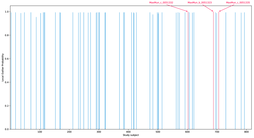
Figure 4. Outlier probability assigned to brain networks of study subjects. Blue indicates outlier probabilities $>0.95$, and red — outlier probabilities $>0.999$. The latter correspond to the subjects MaxMun_c_0051332, MaxMun_b_0051323, and MaxMun_c_0051335. The remaining outlier probabilities are 0.

We replaced the brain network of each subject with its largest component, which did not introduce a significant change to the data: the distribution of the order in the resulting 816 graphs had a mean of about 116.0 and a standard deviation of 0.1.

We estimated the mGH distances in all 332,520 distinct pairs of the connected brain networks. Average graph order and computing time per one pair were distributed as $116.0\pm 0.1$ and $0.40\mathrm{s}\pm 20.29\mathrm{s}$, respectively. The algorithm found exact mGH distances in 78.6% of the graph pairs, with relative error $\eta$ and utility coefficient $\upsilon$ distributed as $0.072\pm 0.139$ and $0.361\pm 0.214$, respectively. We note that using Theorems A and B has reduced the relative error by a factor of 5 on average.

We ran LoOP on the brain networks using their (approximated) pairwise mGH distances $\tilde{d}$. The resulting outlier probability assigned to each brain network (Figure 4) thus measures the abnormality of its shape.

To see if abnormal shape of a brain network corresponds to certain features of the individual, we applied the thresholds of 0.999 and 0.95 to the outlier probabilities. We were unable to identify the corresponding brain network shapes with outlying values of the available measurements, neither for the 3 subjects who scored above the threshold of 0.999 nor for the 54 subjects who scored above 0.95.

To see if the brain networks of subjects within the same diagnostic group tend to have similar shape, we performed cluster analysis based on the mGH distances $\tilde{d}$. We used scipy implementation of hierarchical agglomerative clustering algorithm to split the 816 networks into two clusters (by the number of diagnostic groups in the dataset). The smaller cluster was comprised of the same 3 subjects who scored above the outlier probability threshold of 0.999. Discarding them as outliers and rerunning the analysis resulted in two clusters of 51 and 762 subjects, respectively. The clusters did not show any correspondence with the diagnostic groups, thus providing no evidence that the within-group mGH distances are smaller than the inter-group ones. However, we notice a significant overlap between the 54 subjects with an outlier probability above 0.95 and the cluster of 51 individuals, with 47 people shared between the two groups. This implies that the abnormal brain networks tend to be closer to one another than to the ”regular” brain networks. This observation suggests that abnormality of the brain network shape is influenced by currently unknown features which are not included in the dataset.

We conclude that the algorithm estimates the mGH distance between Spearman’s correlation-based functional brain networks with high accuracy. However, detected shape abnormalities do not seem to correspond to a conclusive pattern related to autism spectrum disorder identification.

6.5. Synthetic networks

To test performance of the algorithm on synthetic networks, we generated 100 graphs per each of Erdős–Rényi (random), Watts–Strogatz (small-world), and Barabási–Albert (scale-free) network models. The order $n$ of each graph was selected uniformly at random between 10 and 200, and other parameters of the model were based on $n$. In the Erdős–Rényi $G(n,p)$ model, the probability $p$ for an edge between a vertex pair to appear was selected uniformly at random between $\frac{0.5\log n}{n}$ and $\frac{1.5\log n}{n}$. In the Watts–Strogatz $G(n,2k,p)$ model, $k$, half of the average vertex degree, was selected uniformly at random between $1$ and $\lfloor 0.5\log^{2}n\rceil$, and the probability $p$ for an edge to get rewired was selected uniformly at random between $\frac{0.5\log n}{n}$ and $\frac{1.5\log n}{n}$. In the Barabási–Albert $G(n,m)$ model, the number of edges $m$ to attach from a new node to the existing nodes was selected uniformly at random between $1$ and $\lfloor\log^{2}n\rceil$.

After generating the graphs, we replaced each of them with its largest connected component. For each set, we estimated the mGH distances in all distinct pairs of the 100 connected graphs therein. Table 3 shows the average graph order in a pair and the performance metrics of the algorithm, aggregated per individual data sets.

	# of	average	computing	exact	relative	utility
	pairs	graph order	time	distances	error $\eta$	coefficient $\upsilon$
Erdős–Rényi	4950	$101.8\pm 56.1$	$0.58\mathrm{s}\pm 0.49\mathrm{s}$	20.1%	$0.222\pm 0.172$	$0.054\pm 0.089$
Watts–Strogatz	4950	$101.5\pm 55.8$	$0.52\mathrm{s}\pm 0.57\mathrm{s}$	50.42%	$0.138\pm 0.170$	$0.004\pm 0.028$
Barabási–Albert	4950	$103.5\pm 37.6$	$0.33\mathrm{s}\pm 0.34\mathrm{s}$	57.1%	$0.131\pm 0.157$	$0.035\pm 0.088$

Table 3. Performance of the algorithm on the synthesized networks. $\mu\pm\sigma$ denotes that distribution of a variable across the graph pairs has a mean of $\mu$ and a standard deviation of $\sigma$.

We note that the algorithm performs significantly worse on the Erdős–Rényi graphs. One possible explanation is that there are fewer identically connected vertices in random graphs than in those resembling real-world networks, which contributes to the combinatorial complexity of the search for distortion-minimizing mappings to obtain the upper bound. Recall from subsection 6.1 that inaccurate computations of the upper bound alone can have a detrimental effect on both $\eta$ and $\upsilon$.

Another interesting observation is that Theorems A and B have smaller utility when applied to the Watts–Strogatz graphs. Recall that a Watts–Strogatz small-world graph is generated from a lattice ring with each node connected to its $2k$ neighbors ($k$ for each side), by randomly rewiring a fraction (roughly, $p$) of its edges. For a small $p$, the rewired edges serve as shortcuts between the otherwise remote vertices and have a highly nonlinear effect on the diameter [WS98]. This allows for high variability in the diameters of generated graphs, thus contributing to the tightness of the baseline lower bounds $b^{\prime}_{L}\buildrel\mathrm{def}\over{=}\frac{1}{2}|\operatorname{diam}X-\operatorname{diam}Y|$.

We conclude that the algorithm performs better on graphs with scale-free and small-world properties, observed in many real-world networks.

7. Conclusion

The main contribution of this work is a feasible method for finding a lower bound on the Gromov–Hausdorff distances between finite metric spaces. The approach, based on the introduced notion of $d$-bounded distance samples, yields a polynomial-time algorithm for estimating the mGH distance. The algorithm is implemented as part of Python scikit-tda library for the case of compact metric spaces induced by unweighted graphs. It is also shown that in the case of unweighted graphs of order $N$ whose diameter scales at most logarithmically with $N$ the algorithm has time complexity $O(N^{3}\log N)$. To the best of our knowledge, this is the first time a feasible algorithm is given for the broad class of graphs occurring in applications.

To test the algorithm’s performance, we applied it to both real and synthesized networks. Among the synthesized networks we tested, the best performance was observed for graphs with scale-free and small-world properties. We have also found that the algorithm performed well on the real-world email exchange, computer, and brain networks. The mGH distance was used to successfully detect outlying shapes corresponding to events of significance. This suggests that the proposed algorithm may be useful for graph shape matching in various application domains.

Appendix A Procedure FindLarge$K$

 

procedure FindLarge$K$($D^{X},d$) $\triangleright$ $O(N^{3})$

$\triangleright$ input: $D^{X}\in\mathbb{R}^{|X|\times|X|}$; $d>0$

$\triangleright$ output: $d$-bounded $K\in\mathrm{\mathbf{K}}_{M(X,d)}(X)$

     $K\leftarrow D^{X}$

     $i\leftarrow\textsc{FindLeastBoundedRow}(K,d)$

     while $i>0$ do $\triangleright$ $i=0$ if and only if $K$ is $d$-bounded

         $K\leftarrow K_{(i)(i)}$ $\triangleright$ remove $i$-th row and column from $K$

         $i\leftarrow\textsc{FindLeastBoundedRow}(K,d)$ $\triangleright$ decide which row to remove next

     end while

     return $K$ $\triangleright$ $K$ is a $d$-bounded distance sample of $X$

end procedure

 

Appendix B Procedure FindLeastBoundedRow

 

procedure FindLeastBoundedRow($A,d$) $\triangleright$ $O(m^{2})$

$\triangleright$ input: $A\in\mathbb{R}^{m\times m}$; $d>0$

$\triangleright$ output: $\begin{cases}0,&\text{if $A$ is $d$-bounded}\\ \min\left\{i\in\langle m\rangle:\text{$\mathrm{row}_{i}(A)$ is "smallest least $d$-bounded"}\right\},&\text{otherwise}\end{cases}$

     $i^{*}\leftarrow 0$

     $n_{i^{*}}\leftarrow 0$

     $s_{i^{*}}\leftarrow 0$

     for $i=1,\ldots,m$ do

         $n_{i}\leftarrow 0$

         $s_{i}\leftarrow 0$

         for $j=1,\ldots,m$ do $\triangleright$ count off-diagonal entries $<d$ and total off-diagonal entries $\geq d$ in $\mathrm{row}_{i}(A)$

              if $i\neq j$ then

                  if $A_{i,j}<d$ then

                       $n_{i}\leftarrow n_{i}+1$

                  else

                       $s_{i}\leftarrow s_{i}+A_{i,j}$

                  end if

              end if

         end for

         if $n_{i}>n_{i^{*}}$ OR ($n_{i}=n_{i^{*}}$ AND $s_{i}<s_{i^{*}}$) then $\triangleright$ choose ”smallest least $d$-bounded” row from the first $i$ rows of $A$

              $i^{*}\leftarrow i$

              $n_{i^{*}}\leftarrow n_{i}$

              $s_{i^{*}}\leftarrow s_{i}$

         end if

     end for

     return $i^{*}$

end procedure

 

Appendix C Procedure SolveFeasibleAssignment

 

procedure SolveFeasibleAssignment($\mathbf{v}$, $\mathbf{u}$, $d$) $\triangleright$ $O(q)$

$\triangleright$ input: $\mathbf{v}\in\mathbb{R}^{p}$ with entries $v_{1}\leq\ldots\leq v_{p}$; $\mathbf{u}\in\mathbb{R}^{q}$ with entries $u_{1}\leq\ldots\leq u_{q}$; $d>0$

$\triangleright$ output: $\begin{cases}\text{TRUE},&\text{if exists injective $f:\langle p\rangle\to\langle q\rangle$ s.t. $\left|v_{k}-u_{f(k)}\right|<d\quad\forall k\in\langle p\rangle$}\\ \text{FALSE},&\text{otherwise}\end{cases}$

     $h\leftarrow 1$

     for $k=1,\ldots,p$ do

         while $|v_{k}-u_{h}|\geq d$ do $\triangleright$ find smallest available $u_{h}$ s.t. $|v_{k}-u_{h}|<d$

              $h\leftarrow h+1$

              if $h>q$ then

                  return FALSE $\triangleright$ no more available entries in $\mathbf{u}$

              end if

         end while

         $h\leftarrow h+1$ $\triangleright$ assign $v_{k}$ to $u_{h}$, making the latter unavailable

     end for

     return TRUE $\triangleright$ $f$ can be constructed

end procedure

 

Appendix D Procedure CheckTheoremB

 

procedure CheckTheoremB($K,D^{Y},d$) $\triangleright$ $O(N^{3})$

$\triangleright$ input: $d$-bounded $K\in\mathrm{\mathbf{K}}_{n}(X)$ for some $n\leq|Y|$; $D^{Y}\in\mathbb{R}^{|Y|\times|Y|}$; $d>0$

$\triangleright$ output: $\begin{cases}\text{TRUE},&\text{if, for some $i\in\langle n\rangle$, $||\mathrm{row}_{i}(K)-\mathrm{row}_{i}(L)||_{\infty}\geq d\quad\forall L\in\mathrm{PSPS}^{n}(D^{Y})$}\\ \text{FALSE},&\text{otherwise}\end{cases}$

     $K\leftarrow\textsc{SortEntriesInRows}(K)$ $\triangleright$ sort entries in every row of $K$

     $D^{Y}\leftarrow\textsc{SortEntriesInRows}(D^{Y})$ $\triangleright$ sort entries in every row of $D^{Y}$

     for $i=1,\ldots,n$ do

         $\texttt{$i$\_satisfies}\leftarrow$ TRUE

         for $j=1,\ldots,|Y|$ do

              if $\textsc{SolveFeasibleAssignment}(\mathrm{row}_{i}(K),\mathrm{row}_{j}(D^{Y}),d)$ then

                  $\texttt{$i$\_satisfies}\leftarrow$ FALSE $\triangleright$ $\exists L\in\mathrm{PSPS}^{n}_{i\leftarrow j}(D^{Y})\quad||\mathrm{row}_{i}(K)-\mathrm{row}_{i}(L)||_{\infty}<d$

              end if

         end for

         if $i$_satisfies then

              return TRUE $\triangleright$ $||\mathrm{row}_{i}(K)-\mathrm{row}_{i}(L)||_{\infty}\geq d\quad\forall L\in\mathrm{PSPS}^{n}(D^{Y})$

         end if

     end for

     return FALSE

end procedure

procedure SortEntriesInRows($A$) $\triangleright$ $O(m^{2}\log m)$

$\triangleright$ input: $A\in\mathbb{R}^{m\times m}$

$\triangleright$ output: $B\in\mathbb{R}^{m\times m}$ s.t. $\forall i\quad\mathrm{row}_{i}(B)$ is a permutation of $\mathrm{row}_{i}(A)$ and $B_{i,1}\leq\ldots\leq B_{i,m}$

     …

end procedure

 

Appendix E Procedure VerifyLowerBound

 

procedure VerifyLowerBound($D^{X},D^{Y},d$) $\triangleright$ $O(N^{3})$

$\triangleright$ input: $D^{X}\in\mathbb{R}^{|X|\times|X|}$; $D^{Y}\in\mathbb{R}^{|Y|\times|Y|}$; $d>0$

$\triangleright$ output: $\begin{cases}\text{TRUE},&\text{if verified that $\widehat{d}_{\mathcal{GH}}(X,Y)\geq\frac{d}{2}$}\\ \text{FALSE},&\text{if couldn't verify it}\end{cases}$

     $K\leftarrow$FindLarge$K$$(D^{X},d)$ $\triangleright$ $K\in\mathbb{R}^{n\times n}$

     $L\leftarrow$FindLarge$K$$(D^{Y},d)$ $\triangleright$ $L\in\mathbb{R}^{m\times m}$

     if $n>|Y|$ OR $m>|X|$ then

         return TRUE $\triangleright$ $\widehat{d}_{\mathcal{GH}}(X,Y)\geq\frac{d}{2}$ from Theorem A

     else if $\textsc{CheckTheoremB}(K,D^{Y},d)$ OR $\textsc{CheckTheoremB}(L,D^{X},d)$ then

         return TRUE $\triangleright$ $\widehat{d}_{\mathcal{GH}}(X,Y)\geq\frac{d}{2}$ from Theorem B

     else

         return FALSE

     end if

end procedure 

Appendix F Procedure FindLowerBound

 

procedure FindLowerBound($D^{X},D^{Y}$) $\triangleright$ $O(N^{7})$

$\triangleright$ input: $D^{X}\in\mathbb{R}^{|X|\times|X|}$; $D^{Y}\in\mathbb{R}^{|Y|\times|Y|}$

$\triangleright$ output: $b_{L}\in\mathbb{R}$ s.t. $\widehat{d}_{\mathcal{GH}}(X,Y)\geq b_{L}$

     $\Delta\leftarrow\emptyset$

     for $i=1,\ldots,|X|$ do $\triangleright$ construct $\Delta$

         for $j=1,\ldots,|X|$ do

              for $k=1,\ldots,|Y|$ do

                  for $l=1,\ldots,|Y|$ do

                       $\Delta\leftarrow\Delta\cup|D^{X}_{i,j}-D^{Y}_{k,l}|$

                  end for

              end for

         end for

     end for

     $\{\delta_{i}\}_{i=1}^{|\Delta|}\leftarrow\textsc{SortSet}(\Delta)$

     for $i=|\Delta|,\ldots,1$ do $\triangleright$ find largest $\frac{\delta_{i}}{2}$ for which the answer is ”yes”

         if $\textsc{VerifyLowerBound}(D^{X},D^{Y},\delta_{i})$ then

              return $\frac{\delta_{i}}{2}$

         end if

     end for

     return $0$

end procedure

procedure SortSet($T$) $\triangleright$ $O(|T|\log|T|)$

$\triangleright$ input: $T\subset\mathbb{R}$

$\triangleright$ output: $\{t_{i}\}_{i=1}^{|T|}$, where $t_{1}<\ldots<t_{|T|}$ and $t_{i}\in T\quad\forall i\in\langle|T|\rangle$

     …

end procedure 

Appendix G Procedure SampleSmallDistortion

 

procedure SampleSmallDistortion($D^{X},D^{Y}$) $\triangleright$ $O(N^{3})$

$\triangleright$ input: $D^{X}\in\mathbb{R}^{|X|\times|X|}$ s.t. $D^{X}_{i,j}=d_{X}(x_{i},x_{j})$; $D^{Y}\in\mathbb{R}^{|Y|\times|Y|}$ s.t. $D^{Y}_{i,j}=d_{Y}(y_{i},y_{j})$

$\triangleright$ output: $\operatorname{dis}R_{\varphi}$, where $R_{\varphi}=\left\{(x,\varphi(x));x\in X\right\}$ for some $\varphi:X\to Y$

     $\pi\leftarrow\textsc{GetRandomOrder}(|X|)$ $\triangleright$ choose order in which to map the points in $X$

     $R_{\varphi}^{(0)}\leftarrow\emptyset$

     for $i=1,\ldots,|X|$ do $\triangleright$ map $x_{\pi(i)}$ at step $i$

         $\delta^{(i)}\leftarrow\infty$ $\triangleright$ initialize $\operatorname{dis}R_{\varphi}^{(i)}$

         $j_{i}\leftarrow 0$

         for $j=1,\ldots,|Y|$ do $\triangleright$ find $y_{j_{i}}$ that minimizes $\operatorname{dis}\Big{(}R_{\varphi}^{(i-1)}\cup\big{\{}(x_{\pi(i)},y_{j_{i}})\big{\}}\Big{)}$

              $\delta\leftarrow\delta^{(i-1)}$

              for $k=1,\ldots,i-1$ do$\triangleright$ find $\operatorname{dis}\Big{(}R_{\varphi}^{(i-1)}\cup\big{\{}(x_{\pi(i)},y_{j})\big{\}}\Big{)}$

                  if $\delta<\big{|}D^{X}_{\pi(i),\pi(k)}-D^{Y}_{j,j_{k}}\big{|}$ then

                       $\delta\leftarrow\big{|}D^{X}_{\pi(i),\pi(k)}-D^{Y}_{j,j_{k}}\big{|}$

                  end if

              end for

              if $\delta<\delta^{(i)}$ then$\triangleright$ choose better $y_{j_{i}}$ candidate

                  $\delta^{(i)}\leftarrow\delta$

                  $j_{i}\leftarrow j$

              end if

         end for

         $R_{\varphi}^{(i)}\leftarrow R_{\varphi}^{(i-1)}\cup\{(x_{\pi(i)},y_{j_{i}})\}$

     end for

     return $\delta^{(|X|)}$

end procedure

procedure GetRandomOrder($n$) $\triangleright$ $O(n)$

$\triangleright$ input: $n\in\mathbb{N}$

$\triangleright$ output: randomly generated permutation $\pi$ of $\langle n\rangle$

     …

end procedure 

Appendix H Procedure FindUpperBound

 

procedure FindUpperBound($D^{X},D^{Y}$) $\triangleright$ $O(sN^{3})$, where $s$ is the total number of sampled mappings

$\triangleright$ input: $D^{X}\in\mathbb{R}^{|X|\times|X|}$; $D^{Y}\in\mathbb{R}^{|Y|\times|Y|}$

$\triangleright$ output: $b_{U}\in\mathbb{R}$ s.t. $\widehat{d}_{\mathcal{GH}}(X,Y)\leq b_{U}$

     $\operatorname{dis}\varphi^{*}\leftarrow\infty$

     $s\leftarrow\textsc{DecideSampleSize}(|X|,|Y|)$ $\triangleright$ number of mappings from $X\to Y$ to sample

     for $i=1,\ldots,s$ do $\triangleright$ randomized sampling from $X\to Y$

         $\operatorname{dis}\varphi\leftarrow\textsc{SampleSmallDistortion}(D^{X},D^{Y})$

         if $\operatorname{dis}\varphi<\operatorname{dis}\varphi^{*}$ then

              $\operatorname{dis}\varphi^{*}\leftarrow\operatorname{dis}\varphi$

         end if

     end for

     $\operatorname{dis}\psi^{*}\leftarrow\infty$

     $s\leftarrow\textsc{DecideSampleSize}(|Y|,|X|)$ $\triangleright$ number of mappings from $Y\to X$ to sample

     for $i=1,\ldots,s$ do $\triangleright$ randomized sampling from $Y\to X$

         $\operatorname{dis}\psi\leftarrow\textsc{SampleSmallDistortion}(D^{Y},D^{X})$

         if $\operatorname{dis}\psi<\operatorname{dis}\psi^{*}$ then

              $\operatorname{dis}\psi^{*}\leftarrow\operatorname{dis}\psi$

         end if

     end for

     return $\frac{1}{2}\max\{\operatorname{dis}\varphi^{*},\operatorname{dis}\psi^{*}\}$

end procedure

procedure DecideSampleSize($n,m$) $\triangleright$ $O(1)$

$\triangleright$ input: $n\in\mathbb{N}$; $m\in\mathbb{N}$

$\triangleright$ output: sample size $s\in\mathbb{N}$ for the population size of $m^{n}$

     $\ldots$

end procedure

References

- [AB02] Réka Albert and Albert-László Barabási. Statistical mechanics of complex networks. Reviews of modern physics, 74(1):47, 2002.
- [AB07] Sophie Achard and Ed Bullmore. Efficiency and cost of economical brain functional networks. PLoS computational biology, 3(2):e17, 2007.
- [ABK15] Yonathan Aflalo, Alexander Bronstein, and Ron Kimmel. On convex relaxation of graph isomorphism. Proceedings of the National Academy of Sciences, 112(10):2942–2947, 2015.
- [AFN+18] Pankaj K Agarwal, Kyle Fox, Abhinandan Nath, Anastasios Sidiropoulos, and Yusu Wang. Computing the gromov-hausdorff distance for metric trees. ACM Transactions on Algorithms (TALG), 14(2):1–20, 2018.
- [BCPP98] Rainer E Burkard, Eranda Cela, Panos M Pardalos, and Leonidas S Pitsoulis. The quadratic assignment problem. In Handbook of combinatorial optimization, pages 1713–1809. Springer, 1998.
- [BDH+06] Horst Bunke, Peter Dickinson, Andreas Humm, Ch Irniger, and Miro Kraetzl. Computer network monitoring and abnormal event detection using graph matching and multidimensional scaling. In Industrial Conference on Data Mining, pages 576–590. Springer, 2006.
- [BK04] H Bunke and M Kraetzl. Classification and detection of abnormal events in time series of graphs. In Data Mining in Time Series Databases, pages 127–148. World Scientific, 2004.
- [Bun97] Horst Bunke. On a relation between graph edit distance and maximum common subgraph. Pattern Recognition Letters, 18(8):689–694, 1997.
- [CCSG+09] Frédéric Chazal, David Cohen-Steiner, Leonidas J Guibas, Facundo Mémoli, and Steve Y Oudot. Gromov-hausdorff stable signatures for shapes using persistence. In Computer Graphics Forum, volume 28, pages 1393–1403. Wiley Online Library, 2009.
- [CFSV04] Donatello Conte, Pasquale Foggia, Carlo Sansone, and Mario Vento. Thirty years of graph matching in pattern recognition. International journal of pattern recognition and artificial intelligence, 18(03):265–298, 2004.
- [CH03] Reuven Cohen and Shlomo Havlin. Scale-free networks are ultrasmall. Physical review letters, 90(5):058701, 2003.
- [Con18] Valentino Constantinou. Pynomaly: Anomaly detection using local outlier probabilities (loop). Journal of Open Source Software, 3(30):845, 2018.
- [COS+98] Eugenio Calabi, Peter J Olver, Chehrzad Shakiban, Allen Tannenbaum, and Steven Haker. Differential and numerically invariant signature curves applied to object recognition. International Journal of Computer Vision, 26(2):107–135, 1998.
- [DMYL+14] Adriana Di Martino, Chao-Gan Yan, Qingyang Li, Erin Denio, Francisco X Castellanos, Kaat Alaerts, Jeffrey S Anderson, Michal Assaf, Susan Y Bookheimer, Mirella Dapretto, et al. The autism brain imaging data exchange: towards a large-scale evaluation of the intrinsic brain architecture in autism. Molecular psychiatry, 19(6):659–667, 2014.
- [FPV14] Pasquale Foggia, Gennaro Percannella, and Mario Vento. Graph matching and learning in pattern recognition in the last 10 years. International Journal of Pattern Recognition and Artificial Intelligence, 28(01):1450001, 2014.
- [Gil62] Paul C Gilmore. Optimal and suboptimal algorithms for the quadratic assignment problem. Journal of the society for industrial and applied mathematics, 10(2):305–313, 1962.
- [Gro81] Mikhael Gromov. Groups of polynomial growth and expanding maps. Publications Mathématiques de l’Institut des Hautes Études Scientifiques, 53(1):53–78, 1981.
- [Gro07] Mikhail Gromov. Metric structures for Riemannian and non-Riemannian spaces. Springer Science & Business Media, 2007.
- [H+16] Reigo Hendrikson et al. Using gromov-wasserstein distance to explore sets of networks. University of Tartu, Master Thesis, 2, 2016.
- [HHZ07] Remco van der Hofstad, Gerard Hooghiemstra, and Dmitri Znamenski. A phase transition for the diameter of the configuration model. Internet Mathematics, 4(1):113–128, 2007.
- [HRD16] Nick Heard and Patrick Rubin-Delanchy. Network-wide anomaly detection via the dirichlet process. In 2016 IEEE Conference on Intelligence and Security Informatics (ISI), pages 220–224. IEEE, 2016.
- [HSSC08] Aric Hagberg, Pieter Swart, and Daniel S Chult. Exploring network structure, dynamics, and function using networkx. Technical report, Los Alamos National Lab.(LANL), Los Alamos, NM (United States), 2008.
- [Kég02] Balázs Kégl. Intrinsic dimension estimation using packing numbers. In NIPS, pages 681–688. Citeseer, 2002.
- [Ken16] Alexander D Kent. Cyber security data sources for dynamic network research. In Dynamic Networks and Cyber-Security, pages 37–65. World Scientific, 2016.
- [KKSZ09] Hans-Peter Kriegel, Peer Kröger, Erich Schubert, and Arthur Zimek. Loop: local outlier probabilities. In Proceedings of the 18th ACM conference on Information and knowledge management, pages 1649–1652, 2009.
- [KO99] Nigel J Kalton and Mikhail I Ostrovskii. Distances between banach spaces. 1999.
- [KS19] Amirali Kazeminejad and Roberto C Sotero. Topological properties of resting-state fmri functional networks improve machine learning-based autism classification. Frontiers in neuroscience, 12:1018, 2019.
- [KVF13] Danai Koutra, Joshua T Vogelstein, and Christos Faloutsos. Deltacon: A principled massive-graph similarity function. In Proceedings of the 2013 SIAM International Conference on Data Mining, pages 162–170. SIAM, 2013.
- [KY04] Bryan Klimt and Yiming Yang. The enron corpus: A new dataset for email classification research. In European Conference on Machine Learning, pages 217–226. Springer, 2004.
- [LCK+06] Hyekyoung Lee, Moo K Chung, Hyejin Kang, Boong-Nyun Kim, Dong Soo Lee, et al. Persistent network homology from the perspective of dendrograms. IEEE Transactions in Medical Imaging, 12:2381–2381, 2006.
- [LCK+11] Hyekyoung Lee, Moo K Chung, Hyejin Kang, Boong-Nyun Kim, and Dong Soo Lee. Computing the shape of brain networks using graph filtration and gromov-hausdorff metric. In International Conference on Medical Image Computing and Computer-Assisted Intervention, pages 302–309. Springer, 2011.
- [LD11] Yaron Lipman and Ingrid Daubechies. Conformal wasserstein distances: Comparing surfaces in polynomial time. Advances in Mathematics, 227(3):1047–1077, 2011.
- [Mém07] Facundo Mémoli. On the use of gromov-hausdorff distances for shape comparison. 2007.
- [Mém09] Facundo Mémoli. Spectral gromov-wasserstein distances for shape matching. In 2009 IEEE 12th International Conference on Computer Vision Workshops, ICCV Workshops, pages 256–263. IEEE, 2009.
- [Mém11] Facundo Mémoli. Gromov–wasserstein distances and the metric approach to object matching. Foundations of computational mathematics, 11(4):417–487, 2011.
- [Mém12] Facundo Mémoli. Some properties of gromov–hausdorff distances. Discrete & Computational Geometry, 48(2):416–440, 2012.
- [Mém13] Facundo Mémoli. The gromov-hausdorff distance: a brief tutorial on some of its quantitative aspects. Actes des rencontres du CIRM, 3(1):89–96, 2013.
- [MS04] Facundo Mémoli and Guillermo Sapiro. Comparing point clouds. In Proceedings of the 2004 Eurographics/ACM SIGGRAPH symposium on Geometry processing, pages 32–40, 2004.
- [PCS16] Gabriel Peyré, Marco Cuturi, and Justin Solomon. Gromov-wasserstein averaging of kernel and distance matrices. In International Conference on Machine Learning, pages 2664–2672. PMLR, 2016.
- [Pin05] Brandon Pincombe. Anomaly detection in time series of graphs using arma processes. Asor Bulletin, 24(4):2, 2005.
- [PW+94] Panos M Pardalos, Henry Wolkowicz, et al. Quadratic Assignment and Related Problems: DIMACS Workshop, May 20-21, 1993, volume 16. American Mathematical Soc., 1994.
- [RBBP+13] Jeffrey D Rudie, JA Brown, Devi Beck-Pancer, LM Hernandez, EL Dennis, PM Thompson, SY Bookheimer, and MJNC Dapretto. Altered functional and structural brain network organization in autism. NeuroImage: clinical, 2:79–94, 2013.
- [RMM+13] Elizabeth Redcay, Joseph M Moran, Penelope Lee Mavros, Helen Tager-Flusberg, John DE Gabrieli, and Susan Whitfield-Gabrieli. Intrinsic functional network organization in high-functioning adolescents with autism spectrum disorder. Frontiers in human neuroscience, 7:573, 2013.
- [RS10] Mikail Rubinov and Olaf Sporns. Complex network measures of brain connectivity: uses and interpretations. Neuroimage, 52(3):1059–1069, 2010.
- [RW02] John W Raymond and Peter Willett. Maximum common subgraph isomorphism algorithms for the matching of chemical structures. Journal of computer-aided molecular design, 16(7):521–533, 2002.
- [SBWG10] Rajmonda Sulo, Tanya Berger-Wolf, and Robert Grossman. Meaningful selection of temporal resolution for dynamic networks. In Proceedings of the Eighth Workshop on Mining and Learning with Graphs, pages 127–136, 2010.
- [Sch17] Felix Schmiedl. Computational aspects of the gromov-hausdorff distance and its application in non-rigid shape matching. Discrete & Computational Geometry, 57(4):854, 2017.
- [SKWB02] Peter Shoubridge, Miro Kraetzl, WAL Wallis, and Horst Bunke. Detection of abnormal change in a time series of graphs. Journal of Interconnection Networks, 3(01n02):85–101, 2002.
- [SMR+08] Kaustubh Supekar, Vinod Menon, Daniel Rubin, Mark Musen, and Michael D Greicius. Network analysis of intrinsic functional brain connectivity in alzheimer’s disease. PLoS computational biology, 4(6):e1000100, 2008.
- [ST19] Nathaniel Saul and Chris Tralie. Scikit-tda: topological data analysis for python. URL https://doi. org/10.5281/zenodo, 2533369, 2019.
- [Stu06] Karl-Theodor Sturm. On the geometry of metric measure spaces. Acta mathematica, 196(1):65–131, 2006.
- [TMLP+02] Nathalie Tzourio-Mazoyer, Brigitte Landeau, Dimitri Papathanassiou, Fabrice Crivello, Olivier Etard, Nicolas Delcroix, Bernard Mazoyer, and Marc Joliot. Automated anatomical labeling of activations in spm using a macroscopic anatomical parcellation of the mni mri single-subject brain. Neuroimage, 15(1):273–289, 2002.
- [Tuz16] Alexey A Tuzhilin. Who invented the gromov-hausdorff distance? arXiv preprint arXiv:1612.00728, 2016.
- [VBBW16] Soledad Villar, Afonso S Bandeira, Andrew J Blumberg, and Rachel Ward. A polynomial-time relaxation of the gromov-hausdorff distance. arXiv preprint arXiv:1610.05214, 2016.
- [Vil03] Cédric Villani. Topics in optimal transportation, volume 58. American Mathematical Soc., 2003.
- [VVGRM12] Nick M Vandewiele, Kevin M Van Geem, Marie-Françoise Reyniers, and Guy B Marin. Genesys: Kinetic model construction using chemo-informatics. Chemical Engineering Journal, 207:526–538, 2012.
- [VWSD10] Bernadette CM Van Wijk, Cornelis J Stam, and Andreas Daffertshofer. Comparing brain networks of different size and connectivity density using graph theory. PloS one, 5(10):e13701, 2010.
- [WS98] Duncan J Watts and Steven H Strogatz. Collective dynamics of ‘small-world’networks. nature, 393(6684):440–442, 1998.