Learning Optimal and Near-Optimal Lexicographic Preference Lists
Abstract
We consider learning problems of an intuitive and concise preference model, called lexicographic preference lists (LP-lists). Given a set of examples that are pairwise ordinal preferences over a universe of objects built of attributes of discrete values, we want to learn (1) an optimal LP-list that decides the maximum number of these examples, or (2) a near-optimal LP-list that decides as many examples as it can. To this end, we introduce a dynamic programming based algorithm and a genetic algorithm for these two learning problems, respectively. Furthermore, we empirically demonstrate that the sub-optimal models computed by the genetic algorithm very well approximate the de facto optimal models computed by our dynamic programming based algorithm, and that the genetic algorithm outperforms the baseline greedy heuristic with higher accuracy predicting new preferences.
Introduction
Preferences are ubiquitous and important to research fields such as recommender systems, decision making and social sciences. In this work, we study preference relations of objects that are combinations of values in discrete attributes. Preference relations vary and the research community has seen promising preference models such as graphical models such as conditional preference networks (?), lexicographic preference trees (?; ?; ?), and lexicographic preference (?; ?), and logical models such as penalty logic (?), possibilistic logic (?), and answer set optimization (?). We focus on a particular lexicographic preference model, called lexicographic preference lists, or LP-lists for short, an intuitive and concise model describing the importance ordering of the attributes and the preference orderings of the values in the attributes (?). In particular, we examine the learning problem of LP-lists for a given description of the set of objects and a given set of examples. This problem is considered in two settings: learning the LP-lists that agree with the maximum, or close to the maximum, number of examples.
Learning optimal LP-lists with maximum number of satisfied examples has been proven NP-hard (?; ?). In this paper, we introduce a dynamic programming based approach that learns optimal LP-lists in exponential time in the number of attributes and the size of attribute domains. Despite this exponentiality, it is a considerable reduction from the factorial time complexity of the brute force algorithm that checks every ordering of attributes and every preference order within each attribute domain. We show the optimality of our algorithm, and present experimental results demonstrating its effectiveness for large domains of objects.
Algorithms to learning near-optimal LP-lists have been proposed in the literature, including the greedy heuristic algorithm (?). Local search algorithms have been used to learn other preference models, e.g., tree-structured conditional preference networks (?). To the best of our knowledge, learning algorithms based on local search techniques have not been applied to learning LP-lists. In this paper, we propose to learn near-optimal LP-lists using a genetic algorithm (?), one of the promising local search algorithms, where LP-lists are straightforward represented as chromosome strings. We conduct empirical evaluation of our genetic algorithm and compare it with the greedy heuristic and our optimal algorithm. Our results suggest that the genetic algorithm performs very close to our optimal algorithm and outperforms the greedy heuristic by a margin.
In the following, we first formally define what LP-lists are. We then present our optimal algorithm using dynamic programming, as well as our near-optimal genetic algorithm. We will discuss our experimental results before we conclude and point to future work.
Lexicographic Preference Lists
Let us denote by a finite set of attributes. Each attribute has a finite domain of values such that . The universe defined by is the Cartesian product of the attribute domains . We call elements in objects. A lexicographic preference list (LP-list) over is a list of attributes in , each labeled by a total order over that attribute domain. Attributes in a LP-list are distinct and a subset of .
Let be an LP-list over , and and two objects in . We say that is at least as good as in , denoted , if (1) for all , or (2) there is such that and for all . Then, we say that is strictly preferred to , denoted , if and , and that is equivalent to , denoted , if and .
Accordingly, given two objects and , and an LP-list , objects can be compared by an LP-list as follows. For each attribute in , starting from the first one, we check if has a better (or worse) value on than . If so, we stop and report (, resp.). Otherwise, and having same value on , we continue to the next attribute. If we finish having checked all attributes, we stop and report . Therefore, this task is done in linear time in the size of the input.
Consider a universe of vehicles of four attributes: BodyType () with values sedan () and truck (), Color () with black (), white () and blue (), Make () with Toyota () and Chevrolet (), and Price () with low (), medium () and high (). An LP-list can be , where is labeled by , by , and by . According to this LP-list, we see that a medium-priced blue Toyota sedan is preferred to a low-priced white Chevrolet sedan, and two differently priced black Chevrolet trucks are equivalent.
Dynamic Programming Algorithm
Given a set of examples and an attribute , we want to compute the optimal local preference ordering of , denoted , that satisfies the maximum number of examples in just by alone.
From we first build a matrix where denotes the number of examples in that prefer to on attribute . Examples with same value of in both are not counted in , so that if . This first step takes both space and time. Then, we use to compute the as follows.
Let be a subset of the domain of , where . We denote by the maximum number of examples in that can be satisfied by any total order on . Thus, we have the following.
Therefore, is the total order on that satisfies examples in . Both and are computed using the following procedure in Algorithm 1, a dynamic programming based procedure recording calculated results in tables and .
We now analyze the space and time complexity of Algorithm 1 as follows. The space complexity results from the matrix , and tables and . Let be the number of values in ’s domain, and the number of examples in . Then, space complexity is . This asymptotic prohibitive space is acceptable, if the size of the attribute’s domain is relatively small, often the case in practice.
To calculate the time complexity, we examine the algorithm closely. We assume structures , , and are constant time accessible. Lines 2 to 5 take time , respectively. The loop from line 6 to line 11 considers all subsets and , for each of which and are computed. Each takes time . So this loop takes time . Then, we have . Therefore, the time complexity of Algorithm 1 is . This is a clear reduction from the factorial performance of the brute-force approach that checks all permutations of .
Let us denote by the set of attributes in labeling the nodes in LPL , by the partial obtained from object restricted to attributes showing up in . Then, we define to be the multi-set of examples obtained from restricted to attributes showing up in .
We say an LPL is optimal to if it satisfies the maximum number of examples in . Inspired by the Held-Karp algorithm (?), we see that, if an LPL is optimal to , then every ’s subtree rooted at is optimal to . Clearly, this property is true because, were the subtree to be not optimal, could be changed to satisfy more examples by altering the order of in .
We devise the Algorithm 2 to learn optimal lexicographic preference lists. It is brute-force enhanced by memorizing the optimal subtrees for all subsets of .
Let us consider the space and time complexities of Algorithm 2. We let be the number of attributes, and the maximum attribute domain size. As with the space complexity, the algorithm uses tables and , and the space designated by the calls to Algorithm 1. The size of is bounded by . This gives us a space complexity of , which is .
Lines 2 to 4 take time respectively. The loop from line 5 to line 10 takes time . Therefore, the time complexity of Algorithm 2 is , which is .
Genetic Algorithm
The idea of the genetic algorithm is inspired from the natural selection theory in biology. Generally, the population’s fitness will increase until a steady state. In such steady state, no improvement can be done once the population has reached this stable state. This state could contain a global or local optimal solution.
Each candidate solution or chromosome is composed of many traits, features, attributes, or simply “genes” with each gene being one value or “allele”. For our learning problem of LP-lists, chromosomes are encoded as follows a string of attributes and values in their domains, where upper-case letters represent attributes and lower-case letters represent values the attributes can be of. Taking the previous example of the LP-list in the cars domain: with the same local preference orderings. Its chromosome representation clearly is “Bst Mtc Cwbk”.
Using the fitness function that returns the number of correctly classified examples by the LP-list, we devise the genetic algorithm as follows. Step 1: create 100 random LP-list as initial chromosomes. Step 2: select the top 50 chromosomes overall according to the fitness function and let them produce two children by crossover and mutation respectively. Step 2 is repeated for 100 generations before termination. In step 2, crossover is achieved by shuffling the ordering of the attributes in the chromosomes, and mutation by shuffling the ordering of values of a randomly chosen attribute.
Results
In this section, we present our empirical analysis of our two algorithm: the dynamic programming based algorithm, for which we call DPA, and the genetic algorithm, which we short-hand to GA.
To evaluate our algorithms DPA and GA, we take the greedy algorithm as a baseline and perform empirical analysis on sets of examples given by hidden randomly generated LP-lists. The examples are produced with a noise percentage of examples that are flipped to create inconsistent examples to simulate practical settings.
Domains of 10 attributes, each of 5 values, are used for our experiments. Thus, the universe contains objects, giving possible examples. We first generate a random LP-list of these attributes with random orderings as their local preferences, and a set of random examples for training and testing. Then, set is processed based on a noise percentage : examples are randomly selected and flipped. We reserve 80% of to train an LP-list model and the other 20% to test it. Our experiments are for of value 15%, and for of size . The instance for every is repeated 5 times and the average accuracies and computational time are reported as follows.
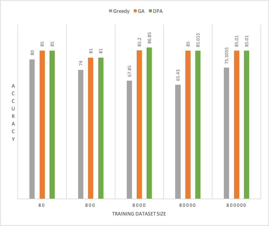
We see, in Figure 1, that DPA obtains the highest accuracy on the testing examples. GA finishes as a very close second, within 1% compared to DPA. Greedy finishes last. We attribute this to the fact that our GA’s stochastic beaming start with multiple LP-lists and generations of improvements of them.
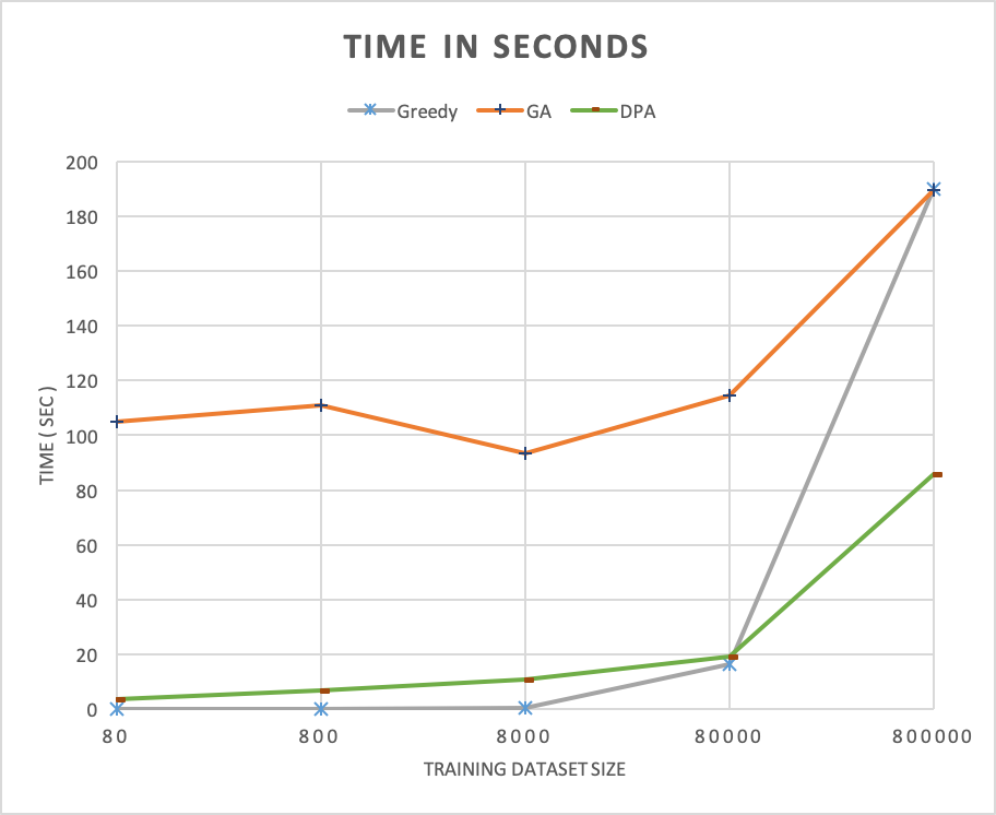
Figure 2 shows the total computational time, including both training and testing, for various training data sizes. Clearly, DPA, despite of its exponential time complexity, outperforms GA on all datasets. This is because the computational time of GA accumulates over generations. Greedy takes the least amount of time until the size of the training set picks up to very large. This is attributed to the larger constant in the asymptotic notion of Greedy than that of DPA. GA takes the most time as it goes through generations of the selecting processes.
Conclusion and Future Work
We studied the learning problems of LP-lists, a preference formalism that is intuitive and concise over objects consisting of categorical attributes. We introduced an algorithm DPA that computes optimal LP-lists that decide the most number of given examples. DPA is based on dynamic programming, and it reduces the factorial time complexity of the pure brute force algorithm to exponential, at a cost of exponential space. Besides, we introduced a genetic algorithm GA for computing near-optimal LP-lists that satisfy as many given examples as it can. To evaluate our algorithms, we conducted substantial experiments showing that, for large example sets of sizes up to 10 million over the universe of over 9 million objects, DPA outperforms GA and baseline Greedy in both testing accuracy and computational time, with GA being a very close second in accuracy. For future work, we plan to perform experimental studies on preferential data generated from real-world datasets such as classification and regression datasets in the machine learning community. We also intend to extend our algorithms to allow learning more general lexicographic preference models (?).
References
- [Allen, Siler, and Goldsmith 2017] Allen, T. E.; Siler, C.; and Goldsmith, J. 2017. Learning tree-structured cp-nets with local search. In Proceedings of the International Florida Artificial Intelligence Research Society Conference.
- [Booth et al. 2010] Booth, R.; Chevaleyre, Y.; Lang, J.; Mengin, J.; and Sombattheera, C. 2010. Learning conditionally lexicographic preference relations. In ECAI, 269–274.
- [Boutilier et al. 2004] Boutilier, C.; Brafman, R.; Domshlak, C.; Hoos, H.; and Poole, D. 2004. CP-nets: A tool for representing and reasoning with conditional ceteris paribus preference statements. Journal of Artificial Intelligence Research 21:135–191.
- [Brewka, Niemelä, and Truszczynski 2003] Brewka, G.; Niemelä, I.; and Truszczynski, M. 2003. Answer set optimization. In IJCAI, volume 3, 867–872.
- [De Saint-Cyr, Lang, and Schiex 1994] De Saint-Cyr, F. D.; Lang, J.; and Schiex, T. 1994. Penalty logic and its link with dempster-shafer theory. In Uncertainty Proceedings 1994. Elsevier. 204–211.
- [Dubois, Lang, and Prade 1994] Dubois, D.; Lang, J.; and Prade, H. 1994. Possibilistic logic 1.
- [Fishburn 1974] Fishburn, P. C. 1974. Exceptional paper—lexicographic orders, utilities and decision rules: A survey. Management science 20(11):1442–1471.
- [Held and Karp 1962] Held, M., and Karp, R. M. 1962. A dynamic programming approach to sequencing problems. Journal of the Society for Industrial and Applied Mathematics 10(1):196–210.
- [Liu and Truszczynski 2013] Liu, X., and Truszczynski, M. 2013. Aggregating conditionally lexicographic preferences using answer set programming solvers. In International Conference on Algorithmic Decision Theory, 244–258. Springer.
- [Liu and Truszczynski 2015] Liu, X., and Truszczynski, M. 2015. Learning partial lexicographic preference trees over combinatorial domains. In Proceedings of the 29th AAAI Conference on Artificial Intelligence (AAAI), 1539–1545. AAAI Press.
- [Liu and Truszczynski 2016] Liu, X., and Truszczynski, M. 2016. Learning partial lexicographic preference trees and forests over multi-valued attributes. In the 2nd Global Conference on Artificial Intelligence, EPiC Series in Computing, 314–328. EasyChair.
- [Liu and Truszczynski 2018] Liu, X., and Truszczynski, M. 2018. Preference learning and optimization for partial lexicographic preference forests over combinatorial domains. In Proceedings of the 10th International Symposium on Foundations of Information and Knowledge Systems (FoIKS). Springer.
- [Mitchell 1998] Mitchell, M. 1998. An introduction to genetic algorithms. MIT press.
- [Schmitt and Martignon 2006] Schmitt, M., and Martignon, L. 2006. On the complexity of learning lexicographic strategies. Journal of Machine Learning Research 7(Jan):55–83.