Emergent Black Hole Dynamics in Critical Floquet Systems

Abstract

While driven interacting quantum matter is generically subject to heating and scrambling, certain classes of systems evade this paradigm. We study such an exceptional class in periodically driven critical $(1+1)$-dimensional systems with a spatially modulated, but disorder-free time evolution operator. Instead of complete scrambling, the excitations of the system remain well-defined. Their propagation is analogous to the evolution along light cones in a curved space-time obtained by two Schwarzschild black holes. The Hawking temperature serves as an order parameter which distinguishes between heating and non-heating phases. Beyond a time scale determined by the inverse Hawking temperature, excitations are absorbed by the black holes resulting in a singular concentration of energy at their center. We obtain these results analytically within conformal field theory, capitalizing on a mapping to sine-square deformed field theories. Furthermore, by means of numerical calculations for an interacting XXZ spin-$\frac{1}{2}$ chain, we demonstrate that our findings survive lattice regularization.

Introduction — Floquet quantum many-body systems provide a rich arena to explore new foundational principles of statistical physics beyond equilibrium. Interest in the field is further spurred on by experimental advances in quantum engineered systems which permit the exploration of Floquet physics in a controlled manner Tang et al. (2018); Reitter et al. (2017). The prevailing paradigm in driven systems is that closed integrable systems converge to steady states described by generalized Gibbs ensembles while interacting Floquet systems heat up to trivial infinite temperature states where all notion of coherence is lost Lazarides et al. (2014). Generically, whether a system heats up or not is intimately linked to notions of integrability, ergodicity, and quantum chaos. A deeper understanding of how a system heats up due the interplay between drive and interactions is still lacking. This is attributable to the limited scope of analytical and numerical methods available to study such complex many body systems.

A pioneering effort in this direction was the recently proposed Floquet conformal field theory (CFT) Wen and Wu (2018a, b), based on a sine square deformation (SSD) of a CFT. SSDs impose a specifc inhomogeneous energy density profile, and were originally proposed as a numerical trick for quantum simulations Gendiar et al. (2009); Hikihara and Nishino (2011); Maruyama et al. (2011). The richness of SSDs was only recently unveiled via studies of both integrable lattice models like quantum spin chains Katsura (2012); Allegra et al. (2016); Dubail et al. (2017) and CFTs in the continuum Ishibashi and Tada (2015); Okunishi (2016a); Wen et al. (2016); Tamura and Katsura (2017); Wen and Wu (2018a, b). It was exploited in Refs. Wen and Wu, 2018a, b, in which a Floquet drive alternating between a generic CFT and its SSD analogue was studied. Analyzing the entanglement entropy, an intriguing phase diagram with transitions between heating and non-heating phases was obtained.

In this letter, we address the question, how does a system heat up ? in this class of systems via an analytical study of dynamical two-point correlation functions in the CFT formalism and a parallel numerical study verifying the surprising robustness of the CFT predictions in a genuine one-dimensional XXZ quantum spin chain at criticality subject to the Floquet-SSD protocol. By analyzing the time-evolution of two-point correlation functions, we show that the heating phase is characterized by the emergence of stroboscopic black hole singularities, which manifest as attractors at two spatial locations towards which all excitations evolve and where energy accumulates indefinitely, irrespective of initial conditions.

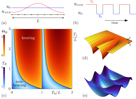
Figure 1: (a) Uniform and SSD Hamiltonian. (b) Floquet drive alternating between the two. (c) Phase diagram (colorbars in log scale). The heating phase is characterized by a Hawking temperature $\Theta_{\mathrm{H}}$, a signature of emergent black holes in the effective dynamics, whose space-time is illustrated in (d). The non-heating phase is characterized by a pseudo-periodicity $T_{E}$, with effective space-time illustrated in (e). The phase diagram is $\tfrac{T_{0}}{L}$ periodic.

We show that the associated Hawking temperature of the black holes serves as de facto order parameter which delineates heating and non-heating phases. The non-heating phase manifests a pseudo-periodicity both in the propagation of excitations as well as energy density.

Floquet-SSD Dynamics — Consider a general inhomogeneous Hamiltonian on a chain of size $L$ obtained by deforming a uniform $(1+1)$-dimensional CFT:

$$\mathcal{H}=\int_{0}^{L}\mathrm{d}xf(x)T_{00}(x).$$ (1)

We denote by $\mathcal{H}_{0}$ the homogeneous CFT where $f\equiv 1$, with energy density $T_{00}$, and by $\mathcal{H}_{\mathrm{SSD}}$ the SSD theory where $f(x)=2\sin^{2}(\tfrac{\pi x}{L})$. We consider a two-step drive protocol, where $\mathcal{H}_{\mathrm{F}}(t)$ alternates between $\mathcal{H}_{\mathrm{SSD}}$ (duration $T_{1}$) and $\mathcal{H}_{0}$ (duration $T_{0}$) as depicted in Fig. 1(a,b). The uniform theory $\mathcal{H}_{0}$ typically describes the low-energy behavior of a quantum chain at criticality and is characterized by a central charge $c$.

The lattice counterpart we explicitly consider is the XXZ spin-$\frac{1}{2}$ chain,

$$H=J\sum_{j=1}^{L-1}f_{j}\Big{(}S_{j}^{x}S_{j+1}^{x}+S_{j}^{y}S_{j+1}^{y}+\Delta S_{j}^{z}S_{j+1}^{z}\Big{)},$$ (2)

The Floquet drive $H_{\mathrm{F}}(t)$ alternates between the the uniform case, $H_{0}$ with $f_{j}\equiv 1$ and the SSD $H_{\mathrm{SSD}}$ where $f_{j}=2\sin^{2}(\tfrac{\pi j}{L})$. For $f_{j}\equiv 1$ and $|\Delta|\leq 1$, the spin chain is critical and the low energy theory is a Luttinger liquid described by a compactified free boson with $c=1$. In what follows, we will demonstrate that the general non-equilibrium exactly solvable CFT-dynamics of $\mathcal{H}_{\mathrm{F}}(t)$ precisely captures the main features of the driven XXZ model $H_{\mathrm{F}}(t)$ that we study numerically.

To probe the dynamics we focus on the unequal time two-point function of the driven CFT $\mathcal{H}_{\mathrm{F}}(t)$, $\langle\phi(x,t)\phi(x_{0},0)\rangle$, where $\phi$ is any primary field (with conformal weight $h$) of the uniform theory $\mathcal{H}_{0}$ Dubail et al. (2017). Though the full time evolution including micromotion can be evaluated, we focus on the stroboscopic evolution, where $t=n(T_{0}+T_{1})$, $n\in\mathbb{N}$. As boundary conditions do not qualitatively affect the ensuing results, we use periodic boundary conditions for computational simplicity. Expectation values are computed in the ground state $|0\rangle$ of the uniform theory. In terms of the Virasoro generators $L_{n}$ and $\overline{L}_{n}$, in the Euclidean framework with imaginary time $\tau$, $\mathcal{H}_{0}=L_{0}+\overline{L}_{0}$, and crucially, $\mathcal{H}_{\mathrm{SSD}}=L_{0}-\tfrac{1}{2}(L_{1}+L_{-1})+\overline{L}_{0}-\tfrac{1}{2}(\overline{L}_{1}+\overline{L}_{-1})$. Such a Hamiltonian is equivalent to a uniform $\mathcal{H}_{0}$ up to an asymptotic $SL(2,\mathbb{R})$ transformation Ishibashi and Tada (2015); Okunishi (2016a); Wen and Wu (2018a). Consequently, time evolution $\mathrm{e}^{-\tau{\mathcal{H}_{\mathrm{SSD}}}}$ is a simple dilation up to a coordinate change. Mapping the coordinates $w=\tau+\mathrm{i}x$ on the cylinder to the complex plane spanned by $z=\mathrm{e}^{2\pi w/L}$, the CFT calculation yields, after analytic continuation to real time (see Supplemental Material for details sup )

$$\langle\phi(x,t)\phi(x_{0},0)\rangle=\left[\Big{(}\frac{2\pi}{L}\Big{)}^{4}\dfrac{\partial\tilde{z}_{n}}{\partial z}\dfrac{\partial\bar{\tilde{z}}_{n}}{\partial\bar{z}}\right]^{h}\langle\phi(\tilde{z}_{n},\bar{\tilde{z}}_{n})\phi(\tilde{z}_{0},\bar{\tilde{z}}_{0})\rangle,$$ (3)

where the two-point function on the right hand side corresponds to the one evaluated in the uniform CFT, namely $\langle\phi(\tilde{z}_{n},\bar{\tilde{z}}_{n})\phi(\tilde{z}_{0},\bar{\tilde{z}}_{0})\rangle=(\tilde{z}_{n}-\tilde{z}_{0})^{-2h}(\bar{\tilde{z}}_{n}-\bar{\tilde{z}}_{0})^{-2h}$. Remarkably, the nontrivial Floquet dynamics is fully encoded in the change of variables, which is essentially a Möbius transformation Wen and Wu (2018b)

$$\tilde{z}_{n}=\dfrac{(\gamma_{1}-\eta^{n}\gamma_{2})z+(\eta^{n}-1)\gamma_{1}\gamma_{2}}{(1-\eta^{n})z+\gamma_{1}\eta^{n}-\gamma_{2}}$$ (4)

where $n$ is the number of drive cycles, $\eta,\gamma_{1},\gamma_{2}$ are complex parameters that depend on $\tfrac{T_{0}}{L}$ and $\tfrac{T_{1}}{L}$ sup . This result is valid for a generic CFT. The central charge enters only via the conformal dimensions of the operators in the correlation function. Moreover, although Eq. (3) captures the stroboscopic dynamics of $\mathcal{H}_{\mathrm{F}}(t)$, it is well defined not only at discrete, but all continuous times – a fact that we will exploit below sup . We now discuss the two distinct regimes of behavior classified by the parameter $\eta$: (i) heating phase for $\eta\in\mathbb{R}^{+}$ (ii) a non-heating phase with $\eta\in\mathbb{C},|\eta|=1$, with $\eta=1$ signalling the transition between the two. The corresponding phase diagram is given in Fig. 1 (c).

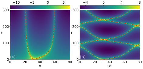
Figure 2: CFT two-point function $|\langle\phi(x,t)\phi(x_{0},0)\rangle|$ for the Floquet drive ($L=80$, $x_{0}=31$, colorbars in log scale). (a) Heating phase ($T_{0}=T_{1}=34$). The excitations are attracted by two black hole singularities at $x_{c}$ and $L-x_{c}$. (b) Non-heating phase ($T_{0}=T_{1}=25$). The dynamics is pseudo-periodic. In both cases, the dashed curves are the null-geodesics of the curved stationary metric.

Heating phase. — In this regime, $\eta\in\mathbb{R}^{+}$, in which case $\tilde{z}_{n}\to\gamma_{1}$ or $\gamma_{2}$ as $n\to\infty$ (depending on the sign of $\eta-1$). A typical two-point function is plotted in Fig. 2 (a). After an initial transient regime during which excitations move quasi-ballistically but start to lose their coherence, the correlation function tends to aggregate at two spatial locations: $x_{c}$ and $L-x_{c}$, independent of the initial condition $x_{0}$. Furthermore, the magnitude of the two point function grows with time indicating that the excitations accumulate indefinitely at the two ‘horizons’. This phenomenon can be interpreted in analogy to black holes emerging from a curved space-time: The two-point function (3) is reduced to a uniform CFT computation in the variable $\tilde{z}_{n}$, for which the metric is flat, namely, $\mathrm{d}s^{2}=\mathrm{d}\tilde{u}_{n}^{2}+\mathrm{d}\tilde{v}_{n}^{2}$ where $\tilde{z}_{n}=\tilde{u}_{n}+\mathrm{i}\tilde{v}_{n}$. The change of coordinates $\tilde{u}_{n}(x,\tau)$, $\tilde{v}_{n}(x,\tau)$ can be computed explicitly from Eq. (4), so we may read-off the corresponding curved metric in the $(x,\tau)$-coordinates. Up to a Weyl transformation and after analytic continuation to real time, one obtains

$$\mathrm{d}s^{2}=\mathrm{d}x^{2}-g(x)\mathrm{d}t^{2}+2h(x)\mathrm{d}x\mathrm{d}t,$$ (5)

in the original coordinates sup . Here, $g$ and $h$ are time-independent real functions. Therefore, the Floquet drive is equivalent to a free propagation in a stationary curved space-time. The null geodesics $\mathrm{d}s^{2}=0$ for such a metric lead to a non-uniform velocity $v(x)=h(x)\pm\sqrt{h(x)^{2}+g(x)}$ and the corresponding trajectories fit perfectly with the analytic two-point function of Fig. 2 (a). In the heating phase, $v(x_{c})=v(L-x_{c})=0$ such that once excitations arrive at these locations, they are permanently trapped.

To explore further the analogy with black holes in this curved space time, we assume that $h(x)=0$, valid for a time-reversal symmetric driving protocol such the $\mathrm{d}x\mathrm{d}t$ term in Eq. (5) vanishes. Consequently, $v(x)=\pm\sqrt{g(x)}$ with $g(x)>0$ and $g(x_{c})=g(L-x_{c})=0$. One infers $x_{c}=\tfrac{L}{2\pi}\arccos(\cos\tfrac{\pi T_{0}}{L}+\tfrac{L}{\pi T_{1}}\sin\tfrac{\pi T_{0}}{L})$ and

$$v(x)=2A\,\dfrac{\sin\big{[}\frac{\pi}{L}(x-x_{c})\big{]}\sin\big{[}\frac{\pi}{L}(x+x_{c})\big{]}}{\cos\big{(}\frac{2\pi x_{c}}{L}\big{)}},$$ (6)

with $A=\tfrac{1+\gamma_{1}^{2}}{\gamma_{1}^{2}-1}\tfrac{L\log\eta}{2\pi\mathrm{i}(T_{0}+T_{1})}\in\mathbb{R}$ sup . Near the horizon $x_{c}$, one finds that at leading order in $x-x_{c}$, $\mathrm{d}s^{2}=-\Theta_{\mathrm{H}}^{2}(x-x_{c})^{2}\mathrm{d}t^{2}+\mathrm{d}x^{2}$. This is a Rindler metric which is equivalent to a Schwarzschild metric in $(1+1)$ dimensions, up to a coordinate change sup . The corresponding Hawking temperature

$$\Theta_{\mathrm{H}}=\frac{|\log{(\eta)}|}{2\pi(T_{0}+T_{1})}$$ (7)

is plotted in Fig. 1 (c). The inverse Hawking temperature provides a timescale after which the excitations are fully trapped at $x=x_{c}$. This timescale diverges at the transition to the non-heating phase, where $\Theta_{\mathrm{H}}\to 0$. A similar expansion of $f$ near $x=L-x_{c}$ leads to a similar metric with the same $\Theta_{\mathrm{H}}$.

Non-heating phase — A typical two-point function in the non-heating phase is plotted in Fig. 2 (b). As expected, the excitations are coherent, resulting in an oscillatory behavior characterized by a new periodicity $T_{E}=2\pi\tfrac{T_{0}+T_{1}}{|\log(\eta)|}$, reminiscent of discrete time crystals Goldstein (2018); Chitra and Zilberberg (2015), see Fig. 1 (c). Notice that $T_{E}$ is in general not an integer multiple of $T_{0}+T_{1}$ so it is only a pseudo-periodicity for the original dynamics. Nevertheless, for some specific values of $T_{0}$ and $T_{1}$ such that $|\log(\eta)|=2\pi p$ with $p\in\mathbb{N}$, $T_{E}$ is indeed an integer multiple of the underlying periodicity of the drive.

The curved space-time interpretation presented earlier is also valid in the non-heating phase i.e., the excitations move ballistically in curved space-time with the stationary metric (5). The main difference is that no black hole singularities exist and the corresponding velocity $v$ for the null geodesics is nonzero everywhere, so the excitation can traverse the entire physical extent of the system. Our analytic results are well described by these geodesics.

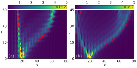
Figure 3: XXZ two-point function $|\langle S_{z}(x,t)S_{z}(x_{0},0)\rangle|$ for the Floquet drive ($\Delta=0.5$, $L=80$). (a) Heating phase ($T_{0}=2$, $T_{1}=4$) (b) Non-heating phase ($T_{0}=-2$, $T_{1}=4$). The dotted curves are the null-geodesics of the curved stationary metric from the CFT approach.

Driven XXZ model — To see if the emergent black holes in the CFT analysis survive in a realistic condensed matter setting, we numerically simulate the XXZ spin chain described in Eq. (2) subject to the Floquet-SSD driving protocol. We use Matrix Product States (MPS) techniques to compute the two-point spin correlation function $\langle G|S^{z}(x,t)S^{z}(x_{0},0)|G\rangle=\langle G|U^{\dagger}(t)S^{z}(x,0)U(t)S^{z}(x_{0},0)|G\rangle$ both in the heating and non-heating phase. This is done using the ITensor library ITe by simply taking the overlap between $U(t)S^{z}(x_{0},0)|G\rangle$ and $S^{z}(x,0)U(t)|G\rangle$, where the unitary evolution is implemented by the sequential application of trotter gates. The numerically computed spin correlation functions are plotted in Fig. 3 and manifest a remarkably good agreement with the stroboscopic CFT predictions for $c=1$ and a compactification radius $R^{2}=\tfrac{2(\pi-\arccos\Delta)}{\pi}$. $S^{z}$ corresponds to a combination of primary fields in the CFT sense. In the heating phase, we clearly see the emergence of the two predicted black-holes singularities and the excitations follow the null geodesics of the curved space time (5). Notice that, for numerical purposes we evolve with $-H_{0}$ instead of $H_{0}$, or equivalently we use a negative time $T_{0}$, which is fine because the phase diagram of Fig. 1 is $\tfrac{T_{0}}{L}$ periodic. In the non-heating phase, the black hole singularities are absent and the geodesics from CFT fit the numerical data well. The effective periodicity $T_{E}$ is not seen in the simulations due to computational limitations on long time physics.

We briefly discuss the role of micromotion within a period. We find that micromotion can indeed lead to additional interesting features both in the CFT as well as the physical system on a lattice. Here, we focused on regimes where micromotion is reduced to small fluctuations around the stroboscopic dynamics, and can be neglected to first order. A thorough study of the role of micromotion will be addressed in future work Choo et al. (2019).

Energy propagation — The time evolution of the energy density $\mathcal{E}(x,t)=\langle T_{00}(x,t)\rangle$ provides yet another remarkable validation of the CFT description of the Floquet-SSD XXZ model. For nontrivial energy dynamics, we choose the ground state $|G\rangle$ of the open chain as the initial state, because for the periodic chain $\mathcal{E}(x,0)\equiv 0$ in the ground state. The discussion is also applicable to other choices of initial states, such as excited states of the periodic chain. The computation of the time evolution of the energy is similar to the two-point function above, except that $T_{00}$ is not primary and boundaries cannot be neglected. Using boundary CFT techniques, we obtain sup

$$\mathcal{E}(x,t)=\alpha\left[\Big{(}\dfrac{\partial\tilde{z}_{n}}{\partial z}\Big{)}^{2}\dfrac{z^{2}}{\tilde{z}_{n}^{2}}+\Big{(}\dfrac{\partial\bar{\tilde{z}}_{n}}{\partial\bar{z}}\Big{)}^{2}\dfrac{\bar{z}^{2}}{\bar{\tilde{z}}_{n}^{2}}\right]-\dfrac{\pi^{2}c}{3L^{2}},$$ (8)

where $\alpha=\tfrac{c}{32}(\tfrac{2\pi}{L})^{2}$, $c$ is the central charge of the theory and $\tilde{z}_{n}$ is given by Eq. (4). In Fig. 4, we show a comparison between the analytically and numerically obtained energy densities. In the non-heating phase, the energy oscillates in time with pseudo-periodicity $T_{E}$, while in the heating phase, energy accumulates indefinitely at the two horizons $x_{c}$ and $L-x_{c}$. Away from these two points, $\mathcal{E}\to 0$ as $t\rightarrow\infty$, whereas $\mathcal{E}(x_{c},t)\sim\mathrm{e}^{4\pi\Theta_{\mathrm{H}}t}$. We see that heating is spatially non-uniform and occurs on the time scale $\Theta_{\mathrm{H}}^{-1}$.

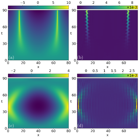
Figure 4: Evolution of energy density $\mathcal{E}(x,t)$ in both phases, comparing CFT computation with numerical simulations ($L=80$, $T_{1}=4$, $\Delta=0.5$). In the heating phase (a and b, $T_{0}=-2$) the energy accumulates indefinitely at the black hole singularities with a time-scale $\Theta_{\mathrm{H}}^{-1}$. In the non-heating phase (c and d, $T_{0}=2$) the energy oscillates in the whole chain with pseudo periodicity $T_{E}$.

Finally, the curved space-time description paradoxically suggests the existence of a well defined Floquet effective Hamiltonian $\mathcal{H}_{\mathrm{eff}}=\int\mathrm{d}xv(x)T_{00}(x)$ in both phases. Note that $v=\sqrt{g}$ is the velocity profile appearing in Eq. (5) (the time-reversal symmetric case where $h=0$). We infer sup

$$\mathcal{H}_{\mathrm{eff}}=\alpha\left[L_{0}-\tfrac{\beta}{2}(L_{1}+L_{-1})+{\bar{L}}_{0}-\tfrac{\beta}{2}({\bar{L}}_{1}+{\bar{L}}_{-1})\right],$$ (9)

where $\beta^{-1}=\cos(\tfrac{\pi T_{0}}{L})+\frac{L}{\pi T_{1}}\sin(\tfrac{\pi T_{0}}{L})$. In the non-heating phase, $|\beta|<1$ and $\mathcal{H}_{\mathrm{eff}}$ is related to the uniform theory $H_{0}$ by an $SL(2,\mathbb{R})$ transformation sup . At the transition, $\beta=1$ and we recover the SSD Hamiltonian. In the heating phase, $|\beta|>1$ and the relation with $H_{0}$ instead requires $SL(2,\mathbb{C})$, leading to drastically different behavior. In particular, we find that $\mathcal{H}_{\mathrm{eff}}$ is unbounded from below in the heating phase as can be seen from the (co)adjoint orbits of $SL(2,\mathbb{R})$ Witten (1988). A simpler way to see this is through conformal quantum mechanics Tada (2018, 2019): any Hamlitonian of the form $aL_{1}+bL_{0}+cL_{-1}$ has a classical counterpart $H=\tfrac{p^{2}}{2}+V(q)$ with $V(q)=\tfrac{1}{2}\tfrac{1}{q^{2}}+\tfrac{c^{(2)}}{8}q^{2}$ with $c^{(2)}=b^{2}-4ac$ the quadratic Casimir invariant. In our case $c^{(2)}=\alpha^{2}(1-\beta^{2})$ so that $V$ is bounded in the non-heating phase and unbounded in the heating phase. Note that in the latter case, the expression for the density of $\mathcal{H}_{\mathrm{eff}}$ bears marked similarities to the one of an entanglement Hamiltonian of a subsystem of size $[x_{c},L-x_{c}]$ Cardy and Tonni (2016).

Discussion — The Floquet drive alternating between a uniform and a SSD CFT provides an exactly solvable non-equilibrium system with a rich phase diagram. We present exact analytical results describing the propagation of excitations as well as energy density in the system. Dynamics in the heating phase are understood by analogy to two black-holes singularities and null geodesics in a curved but stationary space-time geometry. Beyond the timescale fixed by the inverse Hawking temperature, excitations are absorbed by the black holes along with an accumulation of energy at these singularities. We demonstrate numerically that the CFT provides a surprisingly robust description of driven critical spin chains. Cold atomic gases are a promising platform to realize such deformed Hamiltonians Gross and Bloch (2017); Borish et al. (2019), thereby opening up the possibility for experimental observation of emergent black hole dynamics in $(1+1)$-dimensional quantum systems.

Note added — We note that Ref. Fan et al., 2019 also discussed similar results pertaining to accumulation of energy at two points while this manuscript was in preparation.

Acknowledgement — AT thanks Xueda Wen and TN thanks Koji Hashimoto for very helpful discussions. This project has received funding from the European Research Council (ERC) under the European Union’s Horizon 2020 research and innovation program (ERC-StG-Neupert-757867-PARATOP and Marie Sklodowska-Curie grant agreement No 701647).

Supplementary Material

.1 Dynamical Two-point function

In this section we compute the dynamical two-point function defined as $F(x,t;x_{0},0)\equiv\langle\phi(x,t)\phi(x_{0},0)\rangle$ corresponding to a primary field $\phi$ of conformal dimension $h$. The time evolution of the primary is governed by the Floquet Hamiltonian $\mathcal{H}_{\mathrm{F}}(t)$ defined in the main text. We closely follow the strategy employed in Wen and Wu (2018b) wherein the time evolution of the entanglement entropy for a system driven by $\mathcal{H}_{\mathrm{F}}(t)$ was computed. Within this setup, we work in imaginary time $\tau$, and introduce Euclidean coordinates $\omega=\tau+\mathrm{i}x$. Before getting to the computation for an $n$-cycle drive, we describe the 1-cycle drive as a warm-up. The two- point function is

$$F(x,\tau;x_{0},0)=\langle\mathrm{e}^{\tau_{1}\mathcal{H}_{\text{SSD}}}\mathrm{e}^{\tau_{0}\mathcal{H}_{0}}\phi(\omega_{1},\bar{\omega}_{1})\mathrm{e}^{-\tau_{0}\mathcal{H}_{0}}\mathrm{e}^{-\tau_{1}\mathcal{H}_{\text{SSD}}}\phi(\omega_{0},\bar{\omega}_{0})\rangle,$$ (S1)

where $\omega_{1}=0+\mathrm{i}x$, $\omega_{0}=0+\mathrm{i}x_{0}$ and $\tau=\tau_{0}+\tau_{1}$. $\mathcal{H}_{\text{SSD}}$ and $\mathcal{H}_{0}$ are the SSD and uniform Hamiltonian described in the main text. Next, under the conformal mapping $z=\exp\left\{\frac{2\pi\omega}{L}\right\}$, the two-point function transforms as

$$F(x,\tau;x_{0},0)=\left(\frac{2\pi}{L}\right)^{4h}\langle\mathrm{e}^{\tau_{1}\mathcal{H}_{\text{SSD}}}\mathrm{e}^{\tau_{0}\mathcal{H}_{0}}\phi(z_{1},\bar{z}_{1})\mathrm{e}^{-\tau_{0}\mathcal{H}_{0}}\mathrm{e}^{-\tau_{1}\mathcal{H}_{\text{SSD}}}\phi(z_{0},\bar{z}_{0})\rangle.$$ (S2)

To compute the time evolution with $\mathcal{H}_{\text{SSD}}$ in the complex plane, we introduce the so-called Möbius Hamiltonian Okunishi (2016b)

$$\mathcal{H}_{\text{M\"{o}b}(\theta)}=L_{0}-\frac{\tanh(2\theta)}{2}(L_{1}+L_{-1})+\overline{L}_{0}-\frac{\tanh(2\theta)}{2}(\overline{L}_{1}+\overline{L}_{-1}),$$ (S3)

defined for $\theta\in\mathbb{R}^{+}$. Interestingly, there exists an $SL(2,\mathbb{R})$ transformation mapping the Möbius Hamiltonian to a uniform Hamiltonian. Such mapping is explicitly given by

$$\hat{z}=f(z)=\frac{-\cosh(\theta)z+\sinh(\theta)}{\sinh(\theta)z-\cosh(\theta)}.$$ (S4)

In the $\hat{z}$-coordinates, $\mathcal{H}_{\text{M\"{o}b}(\theta)}\propto\frac{2\pi}{L\cosh(2\theta)}(L_{0}+\overline{L}_{0})$. Thus the time evolution with $\mathcal{H}_{\text{M\"{o}b}(\theta)}$ for a time $\tau$ in the $\hat{z}$-coordinates is a simple dilation by a factor $\lambda=\exp\left\{\frac{2\pi\tau}{L\cosh{2\theta}}\right\}$. Then going back to the original coordinates, the whole time evolution with $\mathcal{H}_{\text{M\"{o}b}(\theta)}$ amounts to a simple change of coordinates $z^{\text{new}}_{\theta}(z)=f^{-1}\left(\lambda f(z)\right)$ (in the following of the text we often leave the $z$ dependence of the conformal mappings implicit):

$$z^{\text{new}}_{\theta}(z)=\frac{\left[(1-\lambda)\cosh(2\theta)-(\lambda+1)\right]z+(\lambda-1)\sinh(2\theta)}{(1-\lambda)\sinh(2\theta)z+\left[(\lambda-1)\cosh(2\theta)-(\lambda+1)\right]}.$$ (S5)

The Hamiltonian $\mathcal{H}_{0}$ and $\mathcal{H}_{\text{SSD}}$ can be seen as two different limits of the interpolating Hamiltomian $\mathcal{H}_{\text{M\"{o}b}(\theta)}$. Indeed, $\mathcal{H}_{0}=\mathcal{H}_{\text{M\"{o}b}(0)}$ and $\mathcal{H}_{\text{SSD}}=\mathcal{H}_{\text{M\"{o}b}(\theta\rightarrow\infty)}$. From this observation, it may be deduced that one can first evaluate $e^{\tau_{0}\mathcal{H}_{0}}\phi(\omega,\bar{\omega})e^{-\tau_{0}\mathcal{H}_{0}}$ by applying the method in the case $\theta=0$.

$$e^{\tau_{0}\mathcal{H}_{0}}\phi(\omega_{1},\bar{\omega}_{1})e^{-\tau_{0}\mathcal{H}_{0}}=\left(\frac{2\pi}{L}\right)^{2h}\left[\frac{\partial z^{\text{new}}_{\theta=0}}{\partial z}\bigg{|}_{z_{1}}\frac{\partial\bar{z}^{\text{new}}_{\theta=0}}{\partial\bar{z}}\bigg{|}_{\bar{z}_{1}}\right]^{h}\phi\left(z^{\text{new}}_{\theta=0}(z_{1}),\bar{z}^{\text{new}}_{\theta=0}(z_{1})\right).$$ (S6)

By looking at the expression for $z^{\text{new}}_{\theta}(z)$ in equation (S5), we get $z^{\text{new}}_{\theta=0}(z)=\lambda z$, which is a dilatation in the $z$ plane, as expected for the uniform Hamiltonian $\mathcal{H}_{0}$. Next, we need to evaluate

$$\mathrm{e}^{\tau_{1}\mathcal{H}_{\text{SSD}}}(\mathrm{e}^{\tau_{0}\mathcal{H}_{0}}\phi(z_{1},\bar{z}_{1})\mathrm{e}^{-\tau_{0}\mathcal{H}_{0}})\mathrm{e}^{-\tau_{1}\mathcal{H}_{\text{SSD}}}\propto\mathrm{e}^{\tau_{1}\mathcal{H}_{\text{SSD}}}\phi(\lambda z_{1},\lambda\bar{z}_{1})\mathrm{e}^{-\tau_{1}\mathcal{H}_{\text{SSD}}},$$ (S7)

which can be obtained by using expression of $z^{\text{new}}_{\theta}$ in the limit $\theta\rightarrow\infty$. This just amounts to going to the coordinates $\tilde{z}_{1}$, defined as

$$\tilde{z}_{1}=\lim_{\theta\rightarrow\infty}z^{\text{new}}_{\theta}(\lambda z)=\frac{(1+\frac{\pi\tau_{1}}{L})e^{\frac{2\pi\tau_{0}}{L}}z-\frac{\pi\tau_{1}}{L}}{\frac{\pi\tau_{1}}{L}e^{\frac{2\pi\tau_{0}}{L}}z+(1-\frac{\pi\tau_{1}}{L})}.$$ (S8)

Hence, $\tilde{z}_{1}$ is once again related to $z$ by a Möbius transformation, as expected because it is the obtained via a composition of two (invertible) Möbius transformations. Consequently the time evolution $\mathrm{e}^{\tau_{1}\mathcal{H}_{\text{SSD}}}\mathrm{e}^{\tau_{0}\mathcal{H}_{0}}\phi(z,\bar{z})\mathrm{e}^{-\tau_{0}\mathcal{H}_{0}}\mathrm{e}^{-\tau_{1}\mathcal{H}_{\text{SSD}}}$ for a 1-cycle drive of any primary field of a CFT can be reduced to a normalized Möbius transformation

$$\tilde{z}_{1}=\frac{az+b}{cz+d},$$ (S9)

with

$$\begin{cases}a=(1+\frac{\pi\tau_{1}}{L})e^{\frac{\pi\tau_{0}}{L}},\\ b=-\frac{\pi\tau_{1}}{L}e^{-\frac{\pi\tau_{0}}{L}},\\ c=\frac{\pi\tau_{1}}{L}e^{\frac{\pi\tau_{0}}{L}},\\ d=(1-\frac{\pi\tau_{1}}{L})e^{-\frac{\pi\tau_{0}}{L}}.\par\par\end{cases}$$

Explicitly the two-point function at different times for a 1-cycle drive is

$$\langle\mathrm{e}^{\tau_{1}\mathcal{H}_{\text{SSD}}}\mathrm{e}^{\tau_{0}\mathcal{H}_{0}}\phi(\omega_{1},\bar{\omega}_{1})\mathrm{e}^{-\tau_{0}\mathcal{H}_{0}}\mathrm{e}^{-\tau_{1}\mathcal{H}_{\text{SSD}}}\phi(\omega_{0},\bar{\omega}_{0})\rangle=\left(\frac{2\pi}{L}\right)^{4h}\left[\frac{\partial\tilde{z}_{1}}{\partial z}\bigg{|}_{z_{1}}\frac{\partial\bar{\tilde{z}}_{1}}{\partial\bar{z}}\bigg{|}_{\bar{z}_{1}}\right]^{h}\langle\phi(\tilde{z}_{1},\tilde{z}_{1})\phi(z_{0},\bar{z}_{0})\rangle.$$ (S10)

Therefore we learnt that the time evolution of any primary field during a one cycle of this Floquet drive between $\mathcal{H}_{0}$ and $\mathcal{H}_{\text{SSD}}$ only amounts to a conformal transformation, as seen in (S10). The main task now is to find how to generalize this result to the full Floquet drive with $n$ cycles. Clearly, the $n$-cycle Floquet time evolution will just amount to a change of coordinates to $\tilde{z}_{n}$, defined as

$$\tilde{z}_{n}(z)=\underbrace{(\tilde{z}_{1}\circ...\circ\tilde{z}_{1})}_{n\text{ times}}(z).$$ (S11)

This means that increasing the number of cycles only amounts to composing the 1-cycle transformation with itself.
The $n$-cycle Möbius transformation can be computed by writing the 1-cycle Möbius transformation in its so-called normal form. Introducing the two fixed-points $\gamma_{1}$, $\gamma_{2}$, and the multiplier $\eta$,

$$\begin{cases}\gamma_{1}=\frac{a-d-\sqrt{(a-d)^{2}+4bc}}{2c},\\ \gamma_{2}=\frac{a-d+\sqrt{(a-d)^{2}+4bc}}{2c},\\ \eta=\frac{(a+d)+\sqrt{(a-d)^{2}+4bc}}{a+d-\sqrt{(a-d)^{2}+4bc}}.\end{cases}$$ (S12)

The normal form of $\tilde{z}_{1}$ is then

$$\frac{\tilde{z}_{1}-\gamma_{1}}{\tilde{z}_{1}-\gamma_{2}}=\eta\frac{z-\gamma_{1}}{z-\gamma_{2}}.$$ (S13)

It can be shown that in normal form the $n$-cycle evolution simply amounts to

$$\frac{\tilde{z}_{n}-\gamma_{1}}{\tilde{z}_{n}-\gamma_{2}}=\eta^{n}\frac{z-\gamma_{1}}{z-\gamma_{2}}.$$ (S14)

Then all the stroboscopic time evolution is encoded in the Möbius multiplier $\eta$. This defines different phases, classified by the trace squared of the $1$-cycle transformation Wen and Wu (2018b):

$$\text{Tr}^{2}\begin{pmatrix}a&b\\ c&d\end{pmatrix}=4(1-\Delta).$$ (S15)

Indeed if $\Delta>0$ the associated transformation is elliptic and $\eta$ is a phase: the system does not heat. If $\Delta<0$ the associated transformation is hyperbolic and $\eta$ is a positive number: the system heats. $\Delta=0$ corresponds to a parabolic Möbius transformation, $\eta=1$ and the system is at the phase transition. After analytic continuation, $\Delta$ is written as

$$\Delta=\left[1-\left(\frac{\pi T_{1}}{L}\right)^{2}\right]\sin^{2}\left(\frac{\pi T_{0}}{L}\right)+\frac{\pi T_{1}}{L}\sin\left(\frac{2\pi T_{0}}{L}\right).$$ (S16)

The $n$-cycles Möbius transformation can be explicitly written in terms of the parameters of the system as equation (S17),

$$\tilde{z}_{n}=\frac{\mathfrak{a}z+\mathfrak{b}}{\mathfrak{c}z+\mathfrak{d}},$$ (S17)

with:

$$\begin{cases}\mathfrak{a}=\gamma_{1}-\eta^{n}\gamma_{2},\\ \mathfrak{b}=(\eta^{n}-1)\gamma_{1}\gamma_{2},\\ \mathfrak{c}=1-\eta^{n},\\ \mathfrak{d}=\gamma_{1}\eta^{n}-\gamma_{2}.\par\par\end{cases}$$

Then the stroboscopic time evolution $t=n(T_{0}+T_{1})$ of any primary field $\phi$ can be computed by using this conformal transformation. We stress the fact that here the time evolution is stroboscopic in order to get an analytic handle on the long time dynamics. However, by sacrificing some analytic succinctness we can actually access the full continuous time evolution. The two-point function at different times is directly obtained with equation (S18),

$$\langle\phi(x,t)\phi(x_{0},0)\rangle=\left(\frac{2\pi}{L}\right)^{4h}\left[\frac{\partial\tilde{z}_{n}}{\partial z}\bigg{|}_{z_{1}}\frac{\partial\bar{\tilde{z}}_{n}}{\partial\bar{z}}\bigg{|}_{\bar{z}_{1}}\right]^{h}\langle\phi(\tilde{z}_{n},\bar{\tilde{z}}_{n})\phi(\tilde{z}_{0},\bar{\tilde{z}}_{0})\rangle.$$ (S18)

The correlator $\langle\phi(\tilde{z}_{n},\bar{\tilde{z}}_{n})\phi(\tilde{z}_{0},\bar{\tilde{z}}_{0})\rangle$ can either be computed within the ground state of $\mathcal{H}_{0}$ with open boundary conditions $|G\rangle$, or the $SL(2,\mathbb{C})$ invariant vacuum $|0\rangle$ of the periodic chain. As $|0\rangle$ is an eigenstate of $\mathcal{H}_{\text{SSD}}$, the Floquet dynamics should be trivial when computing correlation functions at equal times, as the SSD time evolution is just a phase. However for dynamical two-point functions $\langle 0|e^{\mathrm{i}\mathcal{H}_{\text{SSD}}t}\phi(x,0)e^{-\mathrm{i}\mathcal{H}_{\text{SSD}}t}\phi(x_{0},0)|0\rangle$ the result should not be trivial as $|\Phi\rangle\equiv\phi(x_{0},0)|0\rangle$ is not an eigenstate of $\mathcal{H}_{\text{SSD}}$ in general. Therefore this choice for the computation of $F(x,t;x_{0},0)$ is legitimate. In the case of open boundary conditions, we need to use the mapping $z\rightarrow\sqrt{z}$ to map the complex plane with a slit to the upper-half plane, and then evaluate the two point function in the upper-half plane Calabrese and Cardy (2007). This introduces some complications regarding branch cuts of the square root mapping. For simplicity, we choose the periodic case, where

$$\langle 0|\phi(\tilde{z}_{n},\bar{\tilde{z}}_{n})\phi(\tilde{z}_{0},\bar{\tilde{z}}_{0})|0\rangle\propto\frac{1}{(z_{0}-\tilde{z}_{n})^{2h}}\frac{1}{(\bar{z}_{0}-\bar{\tilde{z}}_{n})^{2h}}.$$ (S19)

This leads to the final formula for the two-point function at different times for $n$-cycles

$$\langle 0|\phi(x,t)\phi(x_{0},0)|0\rangle=\left(\frac{2\pi}{L}\right)^{4h}\left[\frac{\partial\tilde{z}_{n}}{\partial z}\bigg{|}_{z_{1}}\frac{\partial\bar{\tilde{z}}_{n}}{\partial\bar{z}}\bigg{|}_{\bar{z}_{1}}\right]^{h}\frac{1}{(z_{0}-\tilde{z}_{n})^{2h}}\frac{1}{(\bar{z}_{0}-\bar{\tilde{z}}_{n})^{2h}}.$$ (S20)

It can further be shown that the derivative term simplifies to

$$\frac{\partial\tilde{z}_{n}}{\partial z}\bigg{|}_{z_{1}}\frac{\partial\bar{\tilde{z}}_{n}}{\partial\bar{z}}\bigg{|}_{\bar{z}_{1}}=\frac{(\mathfrak{a}\mathfrak{d}-\mathfrak{b}\mathfrak{c})^{2}}{(\mathfrak{c}^{2}+\mathfrak{d}^{2}+2\mathfrak{c}\mathfrak{d}\cos\left(\frac{2\pi x}{L}\right))^{2}}.$$ (S21)

In the heating phase, $\eta$ is a real positive number, such that $\eta^{n}$ tends either to $0$ or $\infty$ depending on the sign of $\eta-1$, corresponding to $\tilde{z}_{n}$ converging either to $\gamma_{1}$ or $\gamma_{2}$. Then $\langle\phi(\tilde{z}_{n},\bar{\tilde{z}}_{n})\phi(z_{0},\bar{z}_{0})\rangle$ tends to a constant, and the derivative term (S21) is exponentially suppressed for every $x\notin\{x_{c},L-x_{c}\}$, with $x_{c}$ defined by the fixed points: $\gamma_{1/2}=e^{2\pi x_{c}/L}$, where $\gamma_{1/2}$ corresponds to $\gamma_{2}$ if $\tilde{z}_{n}$ converges to $\gamma_{1}$, and vice-versa. This can be seen explicitly in equation (S22),

$$\frac{\partial\tilde{z}_{n}}{\partial z}\bigg{|}_{z_{1}}\frac{\partial\bar{\tilde{z}}_{n}}{\partial\bar{z}}\bigg{|}_{\bar{z}_{1}}=\frac{(\gamma_{1}-\gamma_{2})^{4}}{\left(\eta^{-n}(1+\gamma_{2}^{2}-2\gamma_{2}\cos{\frac{2\pi x}{L}})+2((\gamma_{1}+\gamma_{2})\cos{\frac{2\pi x}{L}}-1-\gamma_{1}\gamma_{2})+\eta^{n}(1+\gamma_{1}^{2}-2\gamma_{1}\cos{\frac{2\pi x}{L}})\right)^{2}}.$$ (S22)

The expression (S22) has a two poles, either in $x_{c}=\frac{L}{2\pi}\arccos\left(\frac{1+\gamma_{2}^{2}}{2\gamma_{2}}\right)$ and $L-x_{c}$ if $\lim_{n\rightarrow\infty}\eta^{n}\rightarrow 0$, or in $x_{c}=\frac{L}{2\pi}\arccos\left(\frac{1+\gamma_{1}^{2}}{2\gamma_{1}}\right)$ and $L-x_{c}$ if $\lim_{n\rightarrow\infty}\eta^{n}\rightarrow\infty$. Therefore $F(x,t;x_{0},0)$ remains finite even at very long times at these two points, for any choice of $x_{0}$. The interpretation is that even after a very long number of driving cycles, the excitations will always arrive at one of these two-points at stroboscopic times. Therefore these particular points, only defined with the choice of $T_{0}/L$ and $T_{1}/L$, act as attractors for the excitations, which will be better understood within a stroboscopic black-hole picture in an effective space-time in the next section. In the non-heating phase, $\eta$ is a phase, and then after analytic continuation the periodicity reads $T_{E}=2\pi\frac{(T_{0}+T_{1})}{|\arg(\eta)|}$. The excitations are then propagating periodically with $T_{E}$. However if $T_{E}/(T_{0}+T_{1})\notin\mathbb{Q}$, the system is pseudo-periodic, as the two-point function is only defined at stroboscopic times.

.2 Effective curved space-time

The two-point function at different times $F(x,t;x_{0},0)$ enables us to get the light-cone propagation of the gapless excitations. For homogeneous Luttinger liquids, the excitations are following straight lines in space-time. However for inhomogeneous Luttinger liquid with spatial deformation $v(x)$, they are following curves, which are nothing more than light-like geodesics in an effective curved space-time specified by the metric $\mathrm{d}s^{2}=\mathrm{d}x^{2}+v(x)^{2}\mathrm{d}\tau^{2}$ Dubail et al. (2017). In the case of the sine-square deformation, the metric is $\mathrm{d}s^{2}=\mathrm{d}x^{2}+\sin^{2}\left(\frac{\pi x}{L}\right)\mathrm{d}\tau^{2}$. Thus, the null geodesics are simply given by the light-like condition $\mathrm{d}s^{2}=0$, giving the propagation of the excitations starting at $x_{0}$: $x_{\pm}(t)=\frac{L}{\pi}\cot^{-1}{\left(\pm\frac{2\pi}{L}t+\cot{\frac{\pi x_{0}}{L}}\right)}$. Therefore it is clear that the excitations never reach the boundaries of the system in this case, as their local group velocity goes to $0$ at the edges.

We now derive the effective space-time metric for the Floquet drive defined at stroboscopic times. We are interested in finding some coordinates $\tilde{z}$ in which the effective metric describing the $n$-cycle Floquet drive is conformally flat, and then going back to the original coordinates $(x,\tau)$ to get the expression of the metric. Such coordinates are called isothermal coordinates and always exist in $(1+1)$-dimensional space-times. For the Floquet drive, they are given by the effective Möbius transformation (S17), so that the metric reads

$$\mathrm{d}s^{2}=\mathrm{d}\tilde{z}_{n}\mathrm{d}\bar{\tilde{z}}_{n}.$$ (S23)

Introducing the real and imaginary parts of $\tilde{z}$

$$\begin{cases}\tilde{u}_{n}(x,\tau)=\text{Re}(\tilde{z}_{n})=\frac{\mathfrak{a}\mathfrak{c}+\mathfrak{b}\mathfrak{d}+(\mathfrak{a}\mathfrak{d}+\mathfrak{b}\mathfrak{c})\cos{\left(\frac{2\pi x}{L}\right)}}{\mathfrak{c}^{2}+\mathfrak{d}^{2}+2\mathfrak{c}\mathfrak{d}\cos{\left(\frac{2\pi x}{L}\right)}},\\ \tilde{v}_{n}(x,\tau)=\text{Im}(\tilde{z}_{n})=\frac{(\mathfrak{a}\mathfrak{d}-\mathfrak{b}\mathfrak{c})\sin{\left(\frac{2\pi x}{L}\right)}}{\mathfrak{c}^{2}+\mathfrak{d}^{2}+2\mathfrak{c}\mathfrak{d}\cos{\left(\frac{2\pi x}{L}\right)}}.\end{cases}$$

The effective metric reads $\mathrm{d}s^{2}=\mathrm{d}\tilde{u}_{n}^{2}+\mathrm{d}\tilde{v}_{n}^{2}$. It is now straightforward to apply the change to ($x$,$\tau$) coordinates. After some computations, the metric takes the familiar form, after analytic continuation:

$$\mathrm{d}s^{2}=\mathrm{e}^{2\sigma(x,\tau)}\left(\mathrm{d}x^{2}-g(x)\mathrm{d}\tau^{2}+2h(x)\mathrm{d}x\mathrm{d}t\right).$$

The value we find for $g(x)$ and $h(x)$ are then given by equations (S24) and (S25)

$$g(x)=\zeta^{2}\prod_{i=1}^{2}\left[1+\gamma_{i}^{2}-2\gamma_{i}\cos{\left(\frac{2\pi x}{L}\right)}\right],$$ (S24)

$$h(x)=\mathrm{i}\zeta(\gamma_{1}\gamma_{2}-1)\sin\left(\frac{2\pi x}{L}\right),$$ (S25)

where $\zeta=-\frac{L}{2\pi\mathrm{i}}\frac{1}{(T_{0}+T_{1})}\frac{\log(\eta)}{(\gamma_{1}-\gamma_{2})}$, and as before $\eta$ is the multiplier of the Möbius transformation, which is a complex exponential in the non-heating phase and a real exponential in the heating phase, and $\gamma_{1}$, $\gamma_{2}$ are the two fixed-points of the 1-cycle Möbius transformation. After analytic continuation, both $g(x)$ and $h(x)$ are real-valued functions.
The Weyl prefactor $\mathrm{e}^{2\sigma(x,\tau)}$ is a positive number before analytic continuation,

$$\mathrm{e}^{2\sigma(x,\tau)}=\frac{4\pi^{2}}{L^{2}}\frac{\eta^{2n}(\gamma_{1}-\gamma_{2})^{4}}{\left(1+\eta^{2n}(1+\gamma_{1}^{2})+\gamma_{2}^{2}-2\eta^{n}(1+\gamma_{1}\gamma_{2})-2(-1+\eta^{n})(\eta^{n}\gamma_{1}-\gamma_{2})\cos(\frac{2\pi x}{L})\right)^{2}}.$$ (S26)

Inverting the Weyl transformation, the metric is finally given by

$$\mathrm{d}s^{2}=\mathrm{d}x^{2}-g(x)\mathrm{d}t^{2}+2h(x)\mathrm{d}x\mathrm{d}t.$$ (S27)

The null geodesics of this $(1+1)$d space-time are uniquely determined by the condition $\mathrm{d}s^{2}=0$. Thus they are the solutions of the equation $2h(x(t))\dot{x}(t)+\dot{x}^{2}(t)-g(x(t))=0$:

$$\pm t(x)=\int_{x_{0}}^{x}dx^{\prime}\frac{1}{\sqrt{h(x^{\prime})^{2}+g(x^{\prime})}\mp h(x^{\prime})}.$$ (S28)

Then the local group velocity of the excitations is $v(x)=h(x)\mp\sqrt{h(x)^{2}+g(x)}$, where the sign corresponds to chiral and anti-chiral excitations. The expression (S27) is not time-reversal invariant because of the off-diagonal term $h(x)$. Only if $\gamma_{1}\gamma_{2}=1$, $h(x)=0$ and the system is time-reversal invariant. This can be fulfilled by starting the drive in a symmetric way. For concreteness, we shift the origin of time by $\frac{T_{0}}{2}$

$$\mathcal{H}_{\mathrm{F}}(t)=\begin{cases}\mathcal{H}_{0}&0<t<\frac{T_{0}}{2},\\ \mathcal{H}_{\text{SSD}}&\frac{T_{0}}{2}<t<\frac{T_{0}}{2}+T_{1},\\ \mathcal{H}_{0}&\frac{T_{0}}{2}+T_{1}<t<\frac{3T_{0}}{2}+T_{1},\\ \text{etc.}\end{cases}$$ (S29)

The associated 1-cycle Möbius transformation is therefore given by the equation

$$\tilde{z}_{1}=\frac{\left(1+\frac{\pi\tau_{1}}{L}\right)\mathrm{e}^{\frac{\pi\tau_{0}}{L}}z-\frac{\pi\tau_{1}}{L}}{\frac{\pi\tau_{1}}{L}z+\left(1-\frac{\pi\tau_{1}}{L}\right)\mathrm{e}^{-\frac{\pi\tau_{0}}{L}}}.$$ (S30)

It is interesting to compare (S30) and (S9). The coefficients $a$ and $d$ are the same as in the non symmetric case, but not $b$ and $c$. Furthermore $bc$ is unchanged. Thus, looking at the definitions of the fixed points and the multiplier, this only redefines the denominators of $\gamma_{1}$ and $\gamma_{2}$, and keeps the multiplier $\eta$ invariant. It can then be shown that $\gamma_{1}\gamma_{2}=1$. Furthermore in the heating phase $|\gamma_{1}|=|\gamma_{2}|=1$, therefore in the time-reversal symmetric situation $\gamma_{1}=\gamma_{2}^{*}$, whereas in the non-heating phase, $\gamma_{1}$ and $\gamma_{2}$ are both real and inverse of each other. In this case, the metric is simplified to $\mathrm{d}s^{2}=\mathrm{d}x^{2}-g(x)\mathrm{d}t^{2}$. Applying the time-reversal condition, one finds that

$$v(x)=[g(x)]^{1/2}=\frac{1}{2\pi\mathrm{i}}\frac{L\log(\eta)}{(T_{0}+T_{1})}\frac{\left(1+\gamma_{1}^{2}-2\gamma_{1}\cos{\frac{2\pi x}{L}}\right)}{\gamma_{1}^{2}-1}.$$ (S31)

This is the effective velocity of the excitations. In the heating phase their local group velocity goes to 0 at two points, which are found to be $x_{c}=\frac{L}{2\pi}\arccos\left(\frac{1+\gamma_{1}^{2}}{2\gamma_{1}}\right)$ and $L-x_{c}$. After analytic continuation, it can be shown that $x_{c}=\tfrac{L}{2\pi}\arccos(\cos\tfrac{\pi T_{0}}{L}+\tfrac{L}{\pi T_{1}}\sin\tfrac{\pi T_{0}}{L})$. Thus $x_{c}\in[0,\frac{L}{2}]$ in the heating phase, and $x_{c}$ is a complex number in the non-heating phase, therefore the velocity never goes to $0$. Thus the heating phase at these two points, the velocity of the excitations vanishes, meaning that their wordlines, following null geodesics of the metric, will tend to one of these two points. We rewrite the metric in the heating phase in terms of the singularity $x_{c}$. We first notice that as $\cos\left(\frac{2\pi x_{c}}{L}\right)=\frac{1}{2}\frac{\gamma_{1}^{2}+1}{\gamma_{1}}$, then the effective deformation is rewritten directly in terms of the singularity

$$v(x)=A\left(1-\frac{\cos\left(\frac{2\pi x}{L}\right)}{\cos\left(\frac{2\pi x_{c}}{L}\right)}\right),$$ (S32)

with $A=\frac{1+\gamma_{1}^{2}}{\gamma_{1}^{2}-1}\frac{1}{2\pi\mathrm{i}(T_{0}+T_{1})}L\log(\eta)$. Using trigonometric formulae, this leads to the desired form of the velocity

$$v(x)=2A\frac{\sin\left[\frac{\pi}{L}(x-x_{c})\right]\sin\left[\frac{\pi}{L}(x+x_{c})\right]}{\cos\left(\frac{2\pi x_{c}}{L}\right)},$$ (S33)

The effective metric can now be easily expressed in terms of the singularity $x_{c}$

$$\mathrm{d}s^{2}=-4A^{2}\frac{\sin^{2}\left[\frac{\pi}{L}(x-x_{c})\right]\sin^{2}\left[\frac{\pi}{L}(x+x_{c})\right]}{\cos^{2}\left(\frac{2\pi x_{c}}{L}\right)}\mathrm{d}t^{2}+\mathrm{d}x^{2}.$$ (S34)

This form is still hard to interpret in terms of Schwarzschild metric. However, by doing an expansion around one of the two singularities, i.e., around $x_{c}$ or $L-x_{c}$, and keeping only the lowest order contribution, only the contribution from one of the singularities should matter and the metric should be simpler. Therefore we expand the expression (S34) around $x_{c}$. At leading order in $x-x_{c}$, we may simplify

$$\sin^{2}\left[\frac{\pi}{L}(x-x_{c})\right]\sin^{2}\left[\frac{\pi}{L}(x+x_{c})\right]\approx\frac{\pi^{2}}{L^{2}}(x-x_{c})^{2}\sin^{2}\left(\frac{2\pi x_{c}}{L}\right)+\mathcal{O}((x-x_{c})^{3}).$$ (S35)

The metric finally simplifies to

$$\mathrm{d}s^{2}=-4A^{2}\tan^{2}\left(\frac{2\pi x_{c}}{L}\right)\frac{\pi^{2}}{L^{2}}(x-x_{c})^{2}\mathrm{d}t^{2}+\mathrm{d}x^{2}.$$ (S36)

This metric is known as the Rindler metric, which describes an accelerated frame transformation of the flat Minkowski metric. Writing $C^{2}=4A^{2}\tan^{2}\left(\frac{2\pi x_{c}}{L}\right)\frac{\pi^{2}}{L^{2}}$, the metric reads $\mathrm{d}s^{2}=-C^{2}(x-x_{c})^{2}\mathrm{d}t^{2}+\mathrm{d}x^{2}$. One can now introduce the following coordinate change: $\frac{C}{2}\left(x-x_{c}\right)^{2}=\left(y-x_{c}\right)$. In the new coordinates, the metric reads

$$\mathrm{d}s^{2}=-2C\left(y-x_{c}\right)\mathrm{d}t^{2}+\frac{1}{2C}\frac{1}{\left(y-x_{c}\right)}\mathrm{d}y^{2}.$$ (S37)

This is the well-known Schwarzschild metric in $(1+1)$ dimensions. Thus expanding our space-time effective metric around one of the two singularities gives (at leading order) a black hole metric. One can also do that for the second singularity by expanding the metric around $L-x_{c}$, to get similar results: $\mathrm{d}s^{2}=-2C\left[y-(L-x_{c})\right]\mathrm{d}t^{2}+\frac{1}{2c}\frac{1}{\left[y-(L-x_{c})\right]}\mathrm{d}y^{2}$.

The Hawking temperature $\Theta_{H}$ can be directly read-off from the expression of the metric as $\Theta_{H}=\frac{C}{2\pi}$. We can finally use the formula $\tan{\left(\frac{2\pi x_{c}}{L}\right)}=\frac{1}{\mathrm{i}}\frac{\gamma_{1}^{2}-1}{\gamma_{1}^{2}+1}$ to conclude that the Hawking temperature is given by $\Theta_{H}=\frac{|\log{(\eta)}|}{2\pi(T_{0}+T_{1})}$.

.3 Effective Hamiltonian

Using the effective metric in the time-reversal symmetric case, we deduce that the stroboscopic effective Hamiltonian is $\mathcal{H}_{\text{eff}}=\int_{0}^{L}v(x)T_{00}(x)\mathrm{d}x$. Using the Fourier decomposition of $v(x)$, given by the equation (S31), and using the definition of the Virasoro generators $L_{n}=\frac{1}{2\pi\mathrm{i}}\oint\mathrm{d}zz^{n+1}T(z)$, we can conclude that the stroboscopic Hamiltonian is

$$\mathcal{H}_{\text{eff}}=\alpha\left[L_{0}-\frac{\beta}{2}(L_{1}+L_{-1})+\overline{L}_{0}-\frac{\beta}{2}(\overline{L}_{1}+\overline{L}_{-1})\right],$$ (S38)

where $\alpha=\frac{1+\gamma_{1}^{2}}{\gamma_{1}^{2}-1}\frac{L}{2\pi\mathrm{i}(T_{0}+T_{1})}\log{(\eta)}$, $\beta=\frac{2\gamma_{1}}{1+\gamma_{1}^{2}}$, which are real numbers. It can further be shown using the expressions of the fixed-points that: $\beta^{-1}=\cos(\frac{\pi T_{0}}{L})+\frac{L}{\pi T_{1}}\sin(\frac{\pi T_{0}}{L})$. Therefore in the heating phase $|\beta|>1$, and in the non-heating phase $|\beta|<1$.

In the case $|\beta|<1$, the effective Hamiltonian is simply the Möbius Hamiltonian (S3). This observation is consistent with the fact that $F(x,t;x_{0},0)$ is periodic in the non-heating phase. Indeed, the propagation of the excitations after a quench with the Möbius Hamiltonian is also periodic, with period $T=\frac{1}{L\cosh(2\theta)}$. Therefore the effective stroboscopic Hamiltonian in the non-heating phase in the time-reversal symmetric case is just an interpolating Hamiltonian between $\mathcal{H}_{0}$ and $\mathcal{H}_{\text{SSD}}$. $\mathcal{H}_{\text{eff}}$ can be further written as the convex combination of the two original Hamiltonians

$$\mathcal{H}_{\text{eff}}=\alpha\left[(1-\beta)\mathcal{H}_{0}+\beta\mathcal{H}_{\text{SSD}}\right].$$ (S39)

Therefore, for $0<\beta<1$, the effective Hamiltonian interpolates between the uniform and the SSD Hamiltonian, as we already understood through the comparison with the Möbius Hamiltonian.

For $\beta>1$, the effective Hamiltonian cannot be understood as an interpolation between the two original Hamiltonians, giving rise to the physics of heating. The effective Hamiltonian in the heating phase can be rewritten, using (S33) as:

$$\mathcal{H}_{\text{eff}}=2L\Theta_{H}\int_{0}^{L}\mathrm{d}x\frac{\sin\left(\frac{\pi}{L}(x-x_{c})\right)\sin\left(\frac{\pi}{L}(x+x_{c})\right)}{\sin\left(\frac{2\pi x_{c}}{L}\right)}T_{00}(x).$$ (S40)

This form of the effective Hamiltonian is reminiscent of the entanglement Hamiltonian $K_{A}$ for a system of finite size $[0,L]$, introduced in Cardy and Tonni (2016), with subsystem $A=(x_{c},L-x_{c})$. However here the Hamiltonian density is integrated over the whole chain. For such entanglement Hamiltonian, an effective local temperature can be defined, diverging at $x_{c}$ and $L-x_{c}$. This is an indication that energy should be absorbed exponentially at these two points.

Finally, looking at the effective deformation $v(x)$ is insightful: in the non-heating phase, we notice that $v(x)$ has no roots. Therefore, it can be thought of as a shifted sine-square, deforming the homogeneous system only smoothly. By going through the phase diagram following the line $T_{0}=T_{1}$, this shifted sine-square will simply tend to the usual sine-square. At the phase transition, the effective Hamiltonian is similar to the sine-square deformation, and has roots at $x_{c}=0$ and $x_{c}=L$. Then, in the heating phase, the two roots will approach symmetrically to the center of the system, giving rise to a cosine-square deformation at the second phase transition , having a single root at $x_{c}=\frac{L}{2}$. Therefore, the effective Hamiltonian in the heating and non-heating phase only interpolates between the sine-square and the cosine-square deformations.

.4 Energy density

The different phases arising within the Floquet CFT were understood in Wen and Wu (2018b) by computing the entanglement entropy, which grows linearly in the heating phase and oscillates with period $T_{E}$ in the non-heating phase. We would like to characterize more precisely these phases by computing the evolution of the energy density $\mathcal{E}(x,t)$ in the system. In particular, we expect to observe an exponential increase of energy in the heating phase precisely at the location of the two singularities $x_{c}$ and $L-x_{c}$, whereas the rest of the system should not absorb energy, to agree with our stroboscopic black hole picture. The energy density $\mathcal{E}(x,t)$ under the Floquet drive is defined by

$$\mathcal{E}(x,t)=\langle\psi(t)|T_{00}(x)|\psi(t)\rangle.$$ (S41)

As usual $T_{00}$ is the energy density of the uniform CFT. $|\psi(t)\rangle=U(t)|G\rangle$ is the time evolved ground state of the uniform Hamiltonian $H_{0}$, with open boundary conditions. We chose open boundary conditions in this case, as in the periodic case $\mathcal{E}(x,t)=0$. In Euclidean coordinates, $T_{00}=T(\omega)+\bar{T}(\bar{\omega})$. The strategy is the same as for the two point function at different times: the first step is to map the strip to the complex plane with a slit, using the exponential mapping

$$\langle G|\mathrm{e}^{\tau\mathcal{H}_{\text{SSD}}}T(\omega)\mathrm{e}^{-\tau\mathcal{H}_{\text{SSD}}}|G\rangle=\left(\frac{\partial z}{\partial\omega}\right)^{2}\langle G|\mathrm{e}^{\tau\mathcal{H}_{\text{SSD}}}T(z)\mathrm{e}^{-\tau\mathcal{H}_{\text{SSD}}}|G\rangle-\frac{\pi^{2}c}{6L^{2}}.$$ (S42)

Then, the usual procedure consists in mapping the complex plane to itself in the Möbius $\tilde{z}_{n}$ coordinates, applying the time evolution and transforming back to the $z$ coordinates. The extra terms coming from the Schwarzian derivative vanish because of $SL(2,\mathbb{R})$ invariance

$$\langle G|\mathrm{e}^{\tau\mathcal{H}_{\text{SSD}}}T(\omega)\mathrm{e}^{-\tau\mathcal{H}_{\text{SSD}}}|G\rangle=\left(\frac{\partial z}{\partial\omega}\right)^{2}\left(\frac{\partial\tilde{z}_{n}}{\partial z}\right)^{2}\langle G|T(\tilde{z}_{n})|G\rangle-\frac{\pi^{2}c}{6L^{2}}.$$ (S43)

The final step is to evaluate the correlation function $\langle G|T(\tilde{z}_{n})|G\rangle$ in a boundary CFT, defined on the complex plane with a slit on the real positive axis. This can be done using a square-root mapping $\sqrt{z}$ to the upper-half plane $\mathbb{H}$. This gives a non-trivial Schwarzian derivative term given by $\{z,\sqrt{z}\}=\dfrac{3}{8z^{2}}$. The upper-half plane can me mapped to the unit disc with a Möbius transformation, therefore, due to rotational symmetry, $\langle G|T(\sqrt{\tilde{z}_{n}})|G\rangle_{\mathbb{H}}=0$ Calabrese and Cardy (2009). Finally, only the Schwarzian derivative term of the square root mapping contributes to the energy density, which before analytic continuation reads

$$\mathcal{E}(x,t)=\frac{c}{32}\left[\left(\frac{\partial z}{\partial\omega}\right)^{2}\left(\frac{\partial\tilde{z}_{n}}{\partial z}\right)^{2}\frac{1}{\tilde{z}_{n}^{2}}+\left(\frac{\partial\bar{z}}{\partial\bar{\omega}}\right)^{2}\left(\frac{\partial\bar{\tilde{z}}_{n}}{\partial\bar{z}}\right)^{2}\frac{1}{\bar{\tilde{z}}_{n}^{2}}\right]-\frac{\pi^{2}c}{3L^{2}},$$ (S44)

for stroboscopic times $t=n(T_{0}+T_{1})$. In the heating phase, as $\mathcal{E}(x_{c},t)\sim\eta^{-2n}$ at long time because of the derivative term $\frac{\partial\bar{\tilde{z}}_{n}}{\partial\bar{z}}$, we conclude that $\mathcal{E}(x_{c},t)\sim\mathrm{e}^{4\pi\Theta_{\mathrm{H}}t}$, such that the Hawking temperature is really the heating rate. Similarly for the other singularity $L-x_{c}$, where the energy is also growing exponentially because of the other derivative term $\frac{\partial\tilde{z}_{n}}{\partial z}$. Therefore the energy density grows exponentially in the heating phase only at the positions of the two black holes, as expected. In the non-heating phase, the energy density oscillates in time with period $T_{E}=2\pi\frac{(T_{0}+T_{1})}{|\arg(\eta)|}$.

References

- Tang et al. (2018) Y. Tang, W. Kao, K.-Y. Li, S. Seo, K. Mallayya, M. Rigol, S. Gopalakrishnan, and B. L. Lev, Phys. Rev. X 8, 021030 (2018).
- Reitter et al. (2017) M. Reitter, J. Näger, K. Wintersperger, C. Sträter, I. Bloch, A. Eckardt, and U. Schneider, Phys. Rev. Lett. 119, 200402 (2017).
- Lazarides et al. (2014) A. Lazarides, A. Das, and R. Moessner, Phys. Rev. Lett. 112, 150401 (2014).
- Wen and Wu (2018a) X. Wen and J.-Q. Wu, Phys. Rev. B97, 184309 (2018a), arXiv:1802.07765 [cond-mat.str-el] .
- Wen and Wu (2018b) X. Wen and J.-Q. Wu, (2018b), arXiv:1805.00031 [cond-mat.str-el] .
- Gendiar et al. (2009) A. Gendiar, R. Krcmar, and T. Nishino, Progress of Theoretical Physics 122, 953 (2009), http://oup.prod.sis.lan/ptp/article-pdf/122/4/953/9681348/122-4-953.pdf .
- Hikihara and Nishino (2011) T. Hikihara and T. Nishino, Phys. Rev. B 83, 060414 (2011).
- Maruyama et al. (2011) I. Maruyama, H. Katsura, and T. Hikihara, Phys. Rev. B 84, 165132 (2011).
- Katsura (2012) H. Katsura, Journal of Physics A: Mathematical and Theoretical 45, 115003 (2012).
- Allegra et al. (2016) N. Allegra, J. Dubail, J.-M. Stéphan, and J. Viti, Journal of Statistical Mechanics: Theory and Experiment 5, 053108 (2016), arXiv:1512.02872 [cond-mat.stat-mech] .
- Dubail et al. (2017) J. Dubail, J.-M. Stéphan, and P. Calabrese, SciPost Physics 3, 019 (2017), arXiv:1705.00679 [cond-mat.str-el] .
- Ishibashi and Tada (2015) N. Ishibashi and T. Tada, Journal of Physics A: Mathematical and Theoretical 48, 315402 (2015).
- Okunishi (2016a) K. Okunishi, Progress of Theoretical and Experimental Physics 2016 (2016a), 10.1093/ptep/ptw060, http://oup.prod.sis.lan/ptep/article-pdf/2016/6/063A02/19302132/ptw060.pdf .
- Wen et al. (2016) X. Wen, S. Ryu, and A. W. W. Ludwig, Phys. Rev. B 93, 235119 (2016).
- Tamura and Katsura (2017) S. Tamura and H. Katsura, Progress of Theoretical and Experimental Physics 2017 (2017), 10.1093/ptep/ptx147, http://oup.prod.sis.lan/ptep/article-pdf/2017/11/113A01/22083375/ptx147.pdf .
- (16) “See supplementary material,” .
- Goldstein (2018) R. E. Goldstein, Physics Today 71, 32 (2018), arXiv:1811.08179 [cond-mat.soft] .
- Chitra and Zilberberg (2015) R. Chitra and O. Zilberberg, Phys. Rev. A 92, 023815 (2015).
- (19) ITensor Library (version 2.0.11) http://itensor.org .
- Choo et al. (2019) K. Choo, B. Lapierre, C. Tauber, A. Tiwari, T. Neupert, and R. Chitra, “Sine-square deformed floquet dynamics for quantum spin chains near criticality,” (2019), in preparation.
- Witten (1988) E. Witten, Communications in Mathematical Physics 114, 1 (1988).
- Tada (2018) T. Tada, PTEP 2018, 061B01 (2018), arXiv:1712.09823 [hep-th] .
- Tada (2019) T. Tada, (2019), arXiv:1904.12414 [hep-th] .
- Cardy and Tonni (2016) J. Cardy and E. Tonni, J. Stat. Mech. 1612, 123103 (2016), arXiv:1608.01283 [cond-mat.stat-mech] .
- Gross and Bloch (2017) C. Gross and I. Bloch, Science 357, 995 (2017).
- Borish et al. (2019) V. Borish, O. Markovic, J. Hines, and M. Schleier-Smith, “Transverse-field ising dynamics in a rydberg-dressed atomic gas,” (2019), to be submitted; private communication.
- Fan et al. (2019) R. Fan, Y. Gu, A. Vishwanath, and X. Wen, arXiv e-prints , arXiv:1908.05289 (2019), arXiv:1908.05289 [cond-mat.str-el] .
- Okunishi (2016b) K. Okunishi, Progress of Theoretical and Experimental Physics 2016, 063A02 (2016b).
- Calabrese and Cardy (2007) P. Calabrese and J. Cardy, J. Stat. Mech. 0706, P06008 (2007), arXiv:0704.1880 [cond-mat.stat-mech] .
- Calabrese and Cardy (2009) P. Calabrese and J. Cardy, J. Phys. A42, 504005 (2009), arXiv:0905.4013 [cond-mat.stat-mech] .