2 mm GISMO Observations of the Galactic Center. I. Dust Emission

Abstract

The Central Molecular Zone (CMZ), covering the inner $\sim 1\arcdeg$ of the Galactic plane has been mapped at 2 mm using the GISMO bolometric camera on the 30 m IRAM telescope. The $21^{\prime\prime}$ resolution maps show abundant emission from cold molecular clouds, from star forming regions, and from one of the Galactic center nonthermal filaments. In this work we use the Herschel Hi-GAL data to model the dust emission across the Galactic center. We find that a single-temperature fit can describe the 160 – 500 µm emission for most lines of sight, if the long-wavelength dust emissivity scales as $\lambda^{-\beta}$ with $\beta\approx 2.25$. This dust model is extrapolated to predict the 2 mm dust emission. Subtraction of the model from the GISMO data provides a clearer look at the 2 mm emission of star-forming regions and the brightest nonthermal filament.

1 Introduction

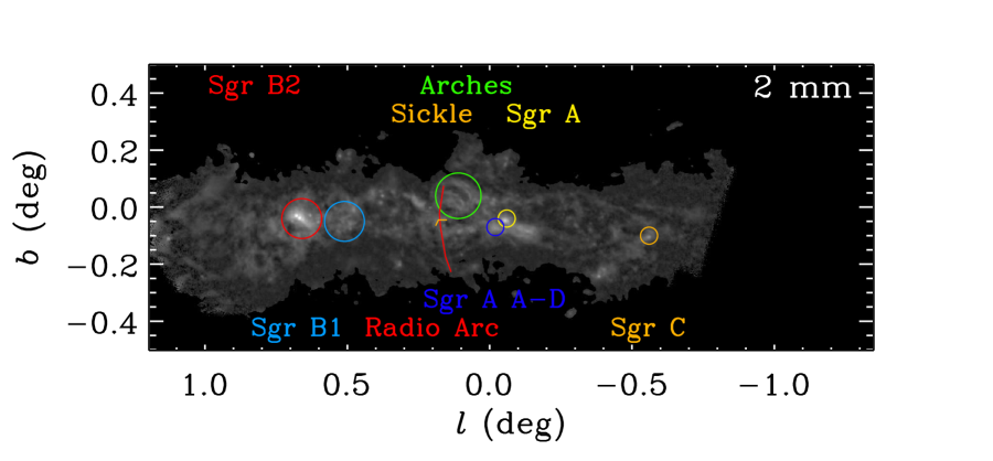
Figure 1: Features in the central molecular zone. Originally defined from longer wavelength radio observations, these features are notable 2 mm sources as well. See Figure 4 for an unadorned version of the 2 mm image.

The Galactic Center presents an interesting challenge to observe and understand because of the huge variety of sources and structures that are superimposed along the line of sight. The line of sight extinction prevents any useful observations at UV or optical wavelengths. The development of infrared, radio, and X-ray observations has provided a clearer view of the Galactic center region. Infrared and radio observations have revealed a central molecular zone (CMZ) within Galactic longitude $|l|\lesssim 1\arcdeg$ or a radius of $\sim 140$ pc of the Galactic center (Morris & Serabyn, 1996). The CMZ contains the largest, densest collection of giant molecular clouds in the Galaxy. Originating from these clouds are numerous star forming regions and young stellar objects with various sizes and ages (e.g Yusef-Zadeh et al., 2009). These in turn have generated large stellar clusters, including the nuclear cluster that swarms around the Galaxy’s central supermassive black hole, and the more outlying Arches and Quintuplet clusters (e.g. Figer et al., 1999, 2002; Genzel et al., 2003). The clusters and individual stars interact with their surrounding medium to produce ionized structures and bubbles (Simpson et al., 1997; Cotera et al., 2005; Simpson et al., 2007). Non-thermal radio structures are seen in the form of supernova remnants and an assortment of individual and bundles of filaments. High-energy (X-ray) observations (e.g. Wang et al., 2002) reveal emission from sources such as accreting compact objects (white dwarfs, neutron stars, or stellar-mass black holes) in binary systems, very hot gas, and colliding stellar winds (Wang et al., 2006; Yusef-Zadeh et al., 2015). Figure 1 provides a guide to the locations of some of the relevant structures in the CMZ.

New observations with new instruments invariably provide insight to one or more of these components of the Galactic Center region. We have carried out a 2 mm continuum survey of the CMZ region using the IRAM 30 m telescope (Baars et al., 1987) paired with the Goddard-IRAM Superconducting 2-Millimeter Observer (GISMO) instrument (Staguhn et al., 2006, 2008). Observations at 2 mm are in an interesting transition zone between mid- and far-IR wavelengths on the one hand (10-500 µm), which are generally dominated by emission from warm and cold interstellar dust, and radio wavelengths on the other hand ($>1$ cm), where the dominant emission mechanisms are free-free emission from ionized gas and synchrotron emission from relativistic electrons. The GISMO survey offers coverage of a wide angular extent (the entire CMZ) with excellent sensitivity and the ability to trace large angular scale emission that higher angular resolution interferometric observations miss. Previous similar surveys and observations are: the BOLOCAM Galactic Plane Survey (Bally et al., 2010; Ginsburg et al., 2013) which covers the entire CMZ at 1.1 mm and is thus dominated by cold dust emission; 3 mm interferometric observations of the inner portion of the CMZ from Sgr A to the Radio Arc by Pound & Yusef-Zadeh (2018), which are sensitive to thermal and non-thermal radio emission and very insensitive to thermal dust emission; 2 mm observations of the Radio Arc region by Reich et al. (2000); and relatively low angular resolution observations at 2 and 3 mm (and other wavelengths) by cosmic microwave background surveys (Culverhouse et al., 2010; Planck Collaboration et al., 2015).

In this paper we present the full 2 mm GISMO image of the Galactic center (Section 2). Here we concentrate on understanding the thermal emission from cold dust in molecular clouds which makes up the bulk of the emission seen at 2 mm. In section 3 we describe the modeling of the Herschel far-IR observations of the CMZ region for the purpose of extrapolating this emission to 2 mm. The comparison of the extrapolated dust emission to the observed 2 mm emission provides a check on the inferred dust properties, temperature and emissivity, and a means to separate 2 mm emission that arises from sources other than cold dust. The comparison between 2 mm free-free emission and thermal emission from dust allows us to make rough estimates of the gas density in regions where these components coexist (Section 4). Investigation of 2 mm emission from the brightest of the nonthermal radio filaments in the Galactic center is presented in a separate paper (Staguhn et al., 2019).

2 Data and Resolution

2.1 GISMO

The 2 mm GISMO bolometric data were collected during April and November 2012. A raster scanning pattern was used for 52 separate scans that are combined here. The total observing time was approximately 8 hours and results in a median integration time of $\sim 1.1$ s pixel^-1. CRUSH (version 2.22-b1) was used for the data reduction (Kovács, 2008), employing the “faint” and “extended” processing flags and 40 “rounds” of iterations to help recover extended emission. The final image has a median noise level of 4.3 mJy beam^-1. The data reduction yields an image spanning roughly $1.2\arcdeg>l>-0.8\arcdeg$ and $|b|<0.3$, with an effective Gaussian beam of $21^{\prime\prime}$ (FWHM). Although these data are collected from a single-dish telescope (not an interferometer), the data reduction necessitated some loss of large-scale structure due to the time-domain filtering required to remove atmospheric variations. There is also no measure of the absolute zero point of the intensity. The GISMO data have been converted from the default units of Jy beam^-1 to MJy sr^-1 to facilitate comparison with the IR maps.

2.2 Herschel

The Herschel data used are data release 1 (DR1) data products, collected and processed as part of the Herschel infrared Galactic Plane Survey (Hi-GAL) survey (Molinari et al., 2016). The data are broad-band images from both the PACS (Poglitsch et al., 2010) and SPIRE (Griffin et al., 2010) instruments. The nominal wavelengths and angular resolution of the data are listed in Table 1. The data were obtained in seven separate fields from the archive and re-joined together to cover the entire region observed by GISMO.

2.3 Convolution

To avoid artifacts in the modeling, we used the procedures of Aniano et al. (2011) to convolve all the images to a common resolution of $37^{\prime\prime}$ (FWHM) which is limited by the 500 µm Herschel SPIRE data (see Table 1). For some later investigation of specific features in the 2 mm image, we convolved images to match GISMO’s $21^{\prime\prime}$ resolution. In such cases one must be cognizant of possible artifacts due to mismatched resolutions of the 350 and 500 $\mu$m data.

The Hi-GAL and GISMO images at $21^{\prime\prime}$ resolution are shown in Figures 2-4. Figure 4 also shows the 19.5 cm radio continuum image of the region from Yusef-Zadeh et al. (2009) which reveals free-free and synchrotron emission.

Table 1: Data Sets Used

Instrument	Wavelength (µm)	FWHM (′′)
PACS	70	5.2
PACS	160	12
SPIRE	250	18
SPIRE	350	25
SPIRE	500	37
GISMO	2 mm	21

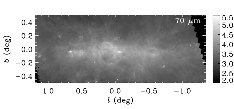
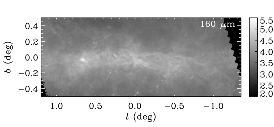
Figure 2: Herschel PACS 70 (top) and 160 $\mu$m (bottom) images from the Hi-GAL survey (Molinari et al., 2016). These are displayed on a logarithmic scale spanning $[100,3.5\times 10^{5}]$ MJy sr^-1. These images are convolved to the $21^{\prime\prime}$ resolution of the GISMO 2 mm data. Emission is dominated by cool dust ($T_{\rm d}\approx 19$ K, see Figure 6), but warmer dust components ($T_{\rm d}$ up to 30 K) in compact and extended H II regions are evident at 70 $\mu$m.

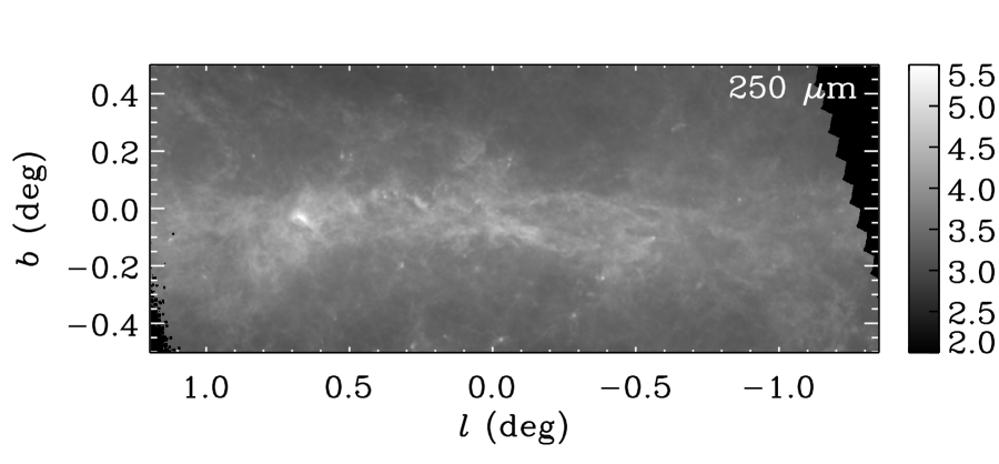
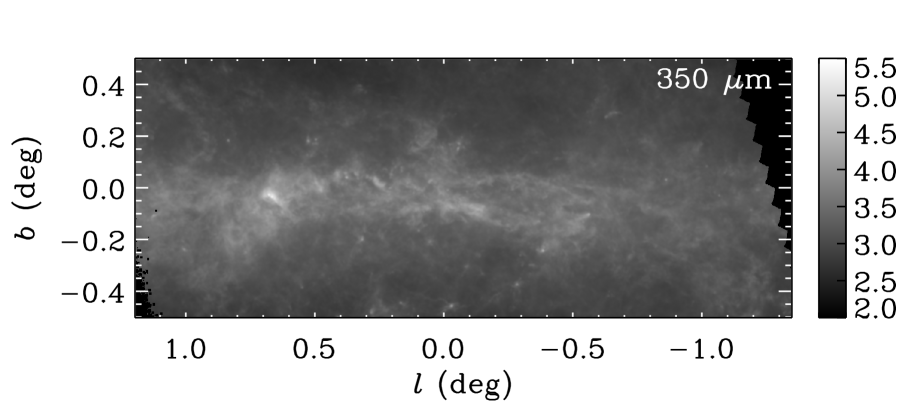
Figure 3: Herschel SPIRE 250 (top) and 350 $\mu$m (bottom) images from the Hi-GAL survey (Molinari et al., 2016). These are displayed on a logarithmic scale spanning $[100,3.5\times 10^{5}]$ MJy sr^-1. The 250 $\mu$m image is convolved to the $21^{\prime\prime}$ resolution of the GISMO 2 mm data. Emission is dominated by cool dust ($T_{\rm d}\approx 19$ K, see Figure 6).

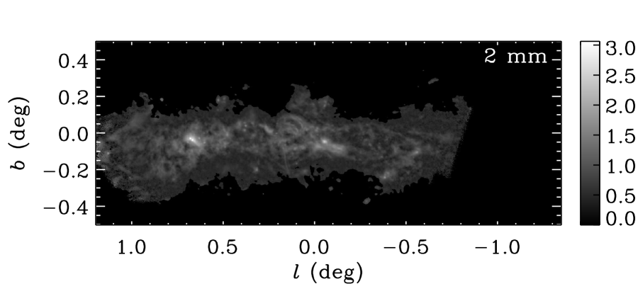
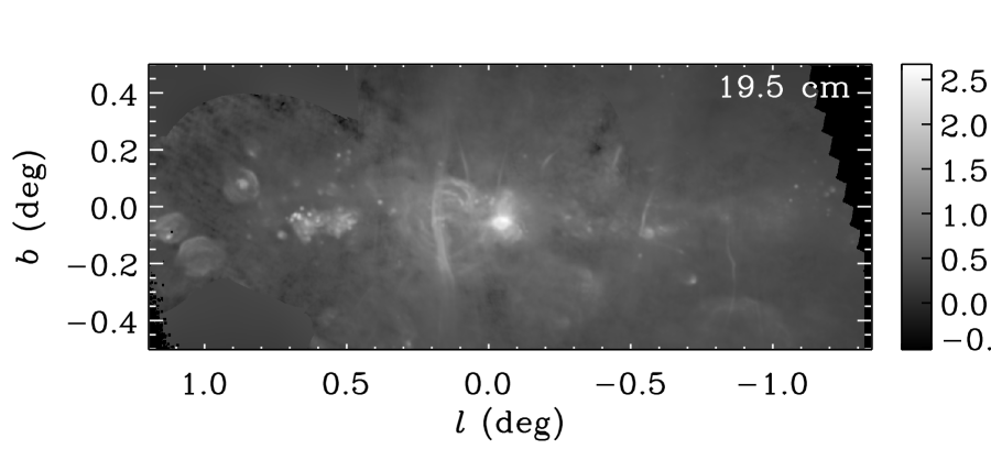
Figure 4: (top to bottom) SPIRE 500 $\mu$m, GISMO 2 mm and VLA 19.5 cm images of the Galactic center region. These are displayed on a logarithmic scale spanning $[100,3.5\times 10^{5}]$, $[1,1150]$, and $[0.3,470]$ MJy sr^-1 respectively (an offset of +3 MJy sr^-1 is applied to the 2 mm image to avoid truncating the negative noise variations of the background). The 19.5 cm image exhibits both thermal (free-free) and non-thermal (synchrotron) sources. The 2 mm image shows features in common with both longer and shorter wavelength images.

3 Dust Emission Models

Inspection of Figure 4 shows that much of the 2 mm emission is correlated with far-IR (500 $\mu$m) emission. However, there are additional features in the 2 mm image that instead correlate with the radio (19.5 cm) emission. In order to characterize each of these emission components, we begin by constructing a model of the dust emission based on the far-IR Herschel data. This model can be used to predict and subtract the dust emission at 2 mm.

3.1 Far-IR emission

The observed surface brightness, $I_{\nu}$, of any pixel is given by

$$I_{\nu}=\int_{0}^{\tau_{\nu}}B_{\nu}(T^{\prime}_{\rm d})e^{-\tau^{\prime}_{\nu}}d\tau^{\prime}_{\nu}$$ (1)

where $B_{\nu}(T^{\prime}_{\rm d})$ is the Planck function, $T^{\prime}_{\rm d}$ and $\tau^{\prime}_{\nu}$ are the temperature and optical depth along the line of sight, and $\tau_{\nu}$ is the total optical depth on the line of sight. Initial examination of the Herschel data indicated that the 160-500 µm data could generally be accurately fit if $T^{\prime}_{\rm d}$ is taken to be constant ($T_{\rm d}$) along the line of sight, while varying for each different line of sight. Therefore we can model the emission as

$$I_{\nu} = B_{\nu}(T_{\rm d})\ \int_{0}^{\tau_{\nu}}e^{-\tau^{\prime}_{\nu}}d\tau^{\prime}_{\nu}$$ (2)

$$= B_{\nu}(T_{\rm d})\ (1-e^{-\tau_{\nu}})$$ (3)

$$\approx B_{\nu}(T_{\rm d})\ \tau_{\nu}$$ (4)

$$= B_{\nu}(T_{\rm d})\ {\cal M}_{d}\ \kappa_{\nu}.$$ (5)

With Equation (4) we assume $\tau_{\nu}\ll 1$, and then express the total optical depth in terms of the mass column density of the dust, ${\cal M}_{d}$, and the mass absorption coefficient of the dust, $\kappa_{\nu}$. At long wavelengths, it is common to characterize the dust emissivity with a power law, such that $\kappa_{\nu}(\lambda)=\kappa_{0}\ \lambda^{-\beta}$.

Therefore the model applied to fit the observed emission at $\lambda_{i}\in[160,\ 250,\ 350,\ 500]$ µm is:

$$I_{\nu}(\lambda_{i})=A\ B_{\nu}(T_{\rm d},\lambda_{i})\ \lambda_{i}^{-\beta}$$ (6)

where the parameters to be determined by $\chi^{2}$ minimization are: the dust temperature, $T_{\rm d}$, the spectral index of the dust emissivity, $\beta$, and the normalization coefficient, $A$, which will be proportional to the product, ${\cal M}_{d}\ \kappa_{0}$. The fitting procedure integrates the model over the appropriate filter bandwidths before comparison to the observed intensities.

Figure 5 shows images of the dust temperature ($T_{\rm d}$) and the dust emissivity index ($\beta$) as derived from these fits. The image of $\chi^{2}$ of the fits is also shown. The image for the normalization ($A$) is very similar to that of $I_{\nu}(500\ \micron)$ and is omitted. On large scales, the derived dust temperature is higher than average in the vicinity of Sgr A and the Arches; it is lower than average in dense molecular clouds that are bright at 500 µm and are sometimes seen in extinction at 70 µm. Large scale variations in the spectral index are correlated with some features, but it’s not clear that consistent trends are present. Figure 6 shows a histogram of $\beta$ that reveals that most of the data are consistent with a mean emissivity index of $\beta\approx 2.25$. A portion of the tails in the histogram, and some more extreme outliers, arise from scattered pixels where poor signal to noise in one or more bands leads to anomalous fits. Figure 7 shows that we find no strong correlation of $T_{\rm d}$ and $\beta$ in this region. We do note that regions with $T_{\rm d}\gtrsim 23$ K generally have lower $\beta$ than most regions, although regions with relatively low $\beta$ can be found at all temperatures. The maps in the lower panels of Figure 7 show that a relatively distinct clustering of points with high $T_{\rm d}$ and low $\beta$ are mostly found in the vicinity of Sgr A and the Arches. Regions with low $T_{\rm d}$ and low $\beta$ are mostly associated with molecular clouds such as the Sgr B2 complex.

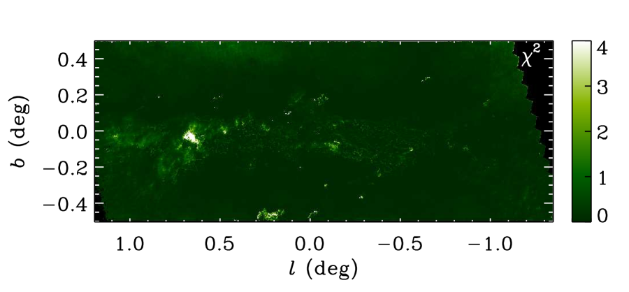
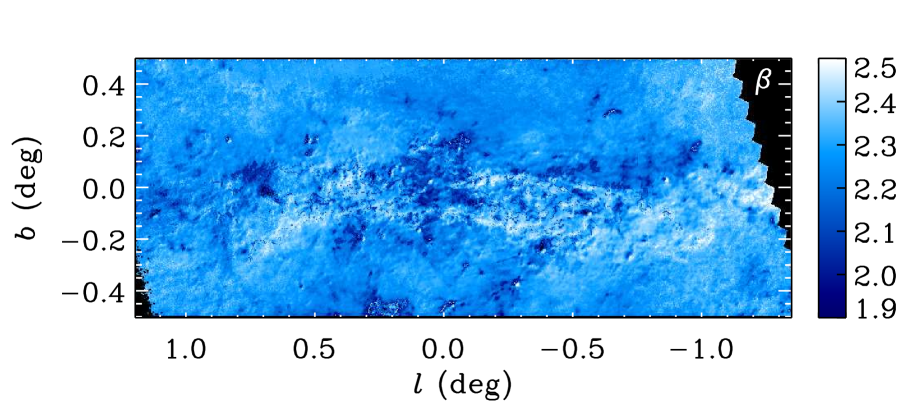
Figure 5: Modeling the 160–500 $\mu$m images using both dust temperature $T_{\rm d}$ (top) and $\beta$ (bottom) as free parameters. The display ranges are [15,35] for $T_{\rm d}$ and [1.9,2.5] for $\beta$. The middle panel shows $\chi^{2}$ for the fit at each pixel on a range of [0,4] (fixed for comparison with later figures). Input data were convolved to $37^{\prime\prime}$ resolution. $T_{\rm d}$ shows cold molecular clouds and warmer regions where strong local heating occurs. Results for $\beta$ are more erratic and show spurious noise-induced features at the pixel scale.

Figure 6: Histograms of the derived $T_{\rm d}$ (top) and $\beta$ (bottom) for each pixel derived using the model in which both are free parameters (See Figure 5). The mean and median values of $\beta$ are 2.27 and 2.28. Based on this distribution, we used a fixed $\beta=2.25$ for subsequent models.

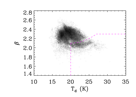
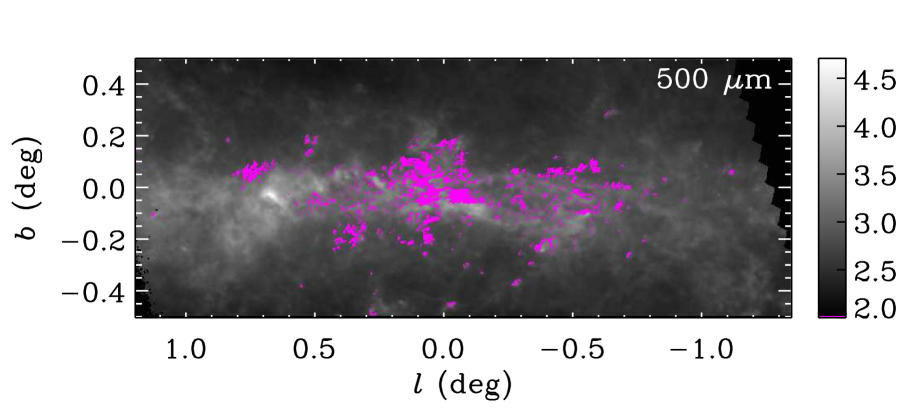
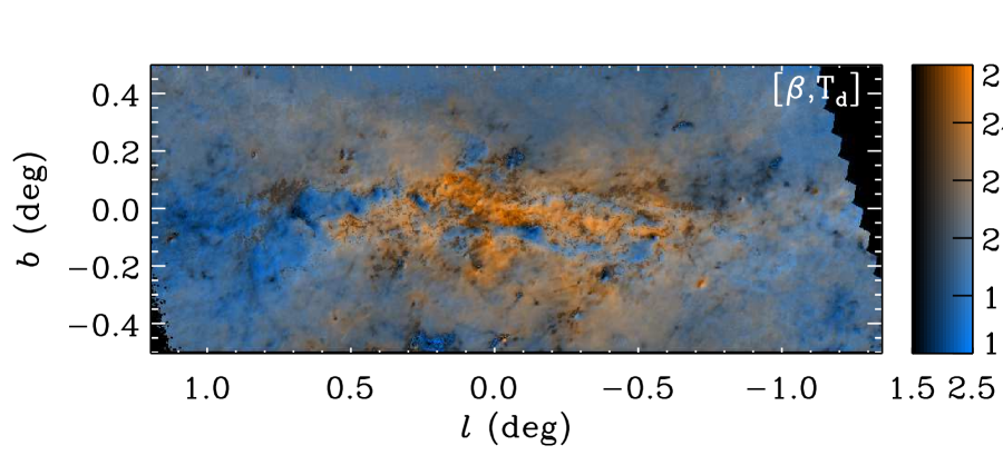
Figure 7: The top panel shows a scatter plot between $T_{\rm d}$ and $\beta$ for all pixels shown in Figure 5. There is no tight correlation between these parameters, although there is the loose trend that regions with high temperatures are likely to have relatively low values of $\beta$. The magenta line separates a branch of points with high $T_{\rm d}$ and low $\beta$ whose locations are marked in magenta on the 500 $\mu$m image in the second panel. The bottom panel shows the simultaneous distribution of $T_{\rm d}$ and $\beta$, encoding $T_{\rm d}$ with color from blue (cold) to orange (warm) and $\beta$ with brightness from low (dark) to high (light) (cf. Fig. 5).

Because of the occasionally spurious fitting results, we next investigated constrained fits where the emissivity index was fixed at $\beta=2.25$. Figure 8 shows that the derived temperatures are similar to those found when $\beta$ is a free parameter, but now there are no spurious pixel-to-pixel variations. The values of $\chi^{2}$ increase somewhat, but there are few major changes. This constrained fit is used as our standard model in further analysis. The third panel in Figure 8 shows the dust mass surface density derived from the fit normalization $A$, assuming $\kappa_{0}=50$ cm² g^-1 at $\lambda_{0}=100$ $\mu$m and that all the dust is at the Galactic center distance of 8.18 kpc (Abuter et al., 2019).

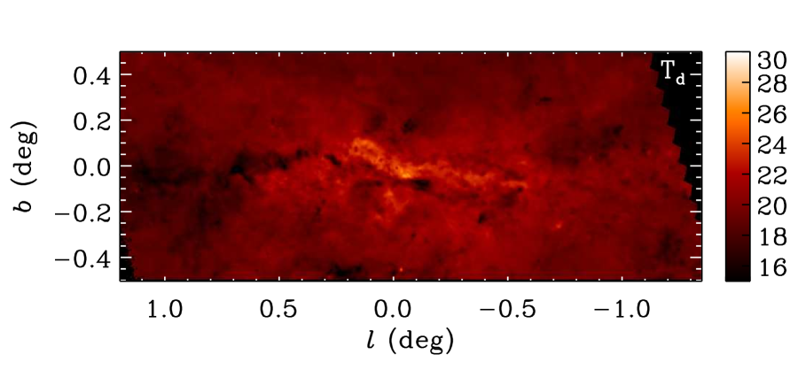
Figure 8: Modeling the 160–500 $\mu$m images using a free dust temperature $T_{\rm d}$ (top) but a fixed $\beta=2.25$. The display range is [15,35] for $T_{\rm d}$. The middle panel shows $\chi^{2}$ for the fit at each pixel on a range of [0,4] (fixed for comparison with other figures). Input data were convolved to $37^{\prime\prime}$ resolution. $T_{\rm d}$ is very similar to the case where $\beta$ is a free parameter, except now all the variations are smoothly continuous without any spurious pixel-to-pixel variations caused by noise. $\chi^{2}$ becomes worse at some locations (cf. Figure 5), as expected for a more constrained model. The bottom panel shows the model’s dust mass surface density (proportional to the normalization parameter $A$). The image is logarithmically scaled from 0.01 – 1 $M_{\sun}$ asec^-2. Contours are at [0.04, 0.08, 0.3] $M_{\sun}$ asec^-2.

For comparison, we also performed a constrained fit using a more conventional value of $\beta=2.0$. The temperature distribution (Figure 9) is very similar to that found for $\beta=2.25$ except it is systematically slightly warmer, as would be expected for a flatter emissivity index. There are a few isolated regions where $\chi^{2}$ is distinctly lower for the flatter spectral index. Many of these are associated with higher latitude features that appear as IR dark clouds at shorter wavelengths ($\lambda\lesssim 70$ $\mu$m). The high latitude and extreme darkness of these clouds suggest that they are in the foreground relative to the Galactic center.

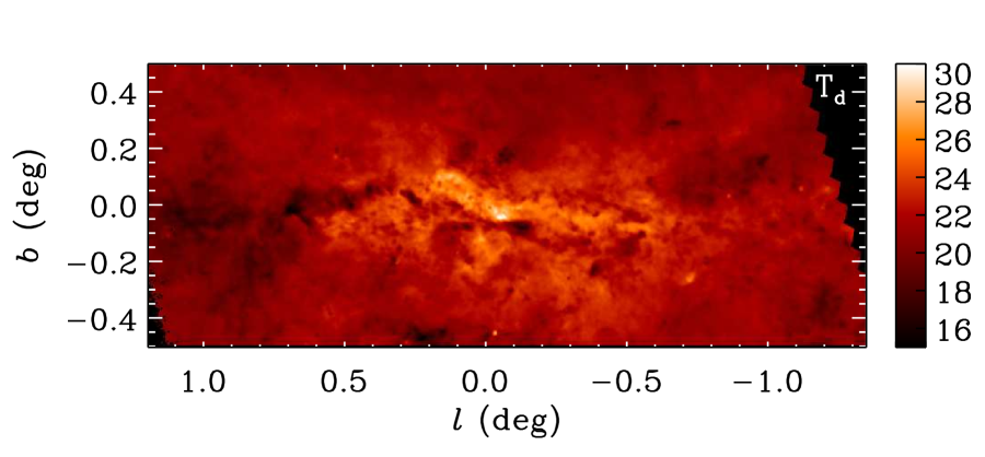
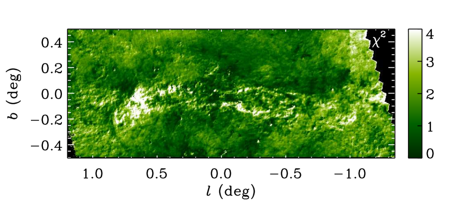
Figure 9: Modeling the 160–500 $\mu$m images using a free dust temperature $T_{\rm d}$ (top) but a fixed $\beta=2.00$. The display range is [15,35] for $T_{\rm d}$. The lower panel shows $\chi^{2}$ for the fit at each pixel on a range of [0,4] (fixed for comparison with other figures). Input data were convolved to $37^{\prime\prime}$ resolution. $T_{\rm d}$ is similar to, but systematically higher than the case where $\beta=2.25$. $\chi^{2}$ is now much worse at all locations (cf. Figures 5 and 8), indicating that the Herschel data alone require $\beta>2.0$. Curiously, it is in this $\chi^{2}$ image that a circular feature at $(l,b)=(-0.35,0.18)$ is most easily distinguished.

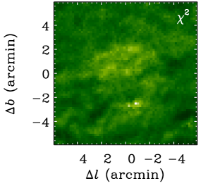
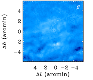
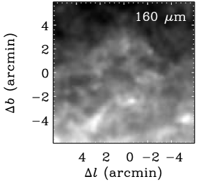
Figure 10: Magnified images of an unusual circular structure as revealed by fitting deviations ($\chi^{2}$), emissivity index ($\beta$), and 160 $\mu$m emission (left to right). The structure is centered at $(l,b)=(359.65,+0.18)$. The structure seems to be largely defined by unusual dust properties (See Section 3.1).

There is a peculiar shell-like feature in the $\chi^{2}$ map for $\beta=2.0$ (Figure 9). It is $3^{\prime}$ in radius at $(l,b)=(359.65,+0.18)$ and is also distinguished from its surroundings by a slightly steeper value of $\beta\sim 2.35$ (Figure 5). Figure LABEL:fig:circle_provides_a_magnified_view_of_this_region. The structure is not particularly distinctive, but can be discerned, in the Herschel 160 - 500 $\mu$m intensity maps. The structure is not evident in Spitzer images at 3.6 - 24 $\mu$m or at radio wavelengths. While there are many possible candidates for a central star to this structure, none are particularly distinguished by exceptional colors or brightnesses at 1.25 - 24 $\mu$m.

3.2 2 mm and 70 µm emission

We extrapolate the emission model fit to the 160 – 500 µm data to predict the dust emission at 2 mm and at 70 µm. The extrapolated intensity maps are shown in Figure 11.

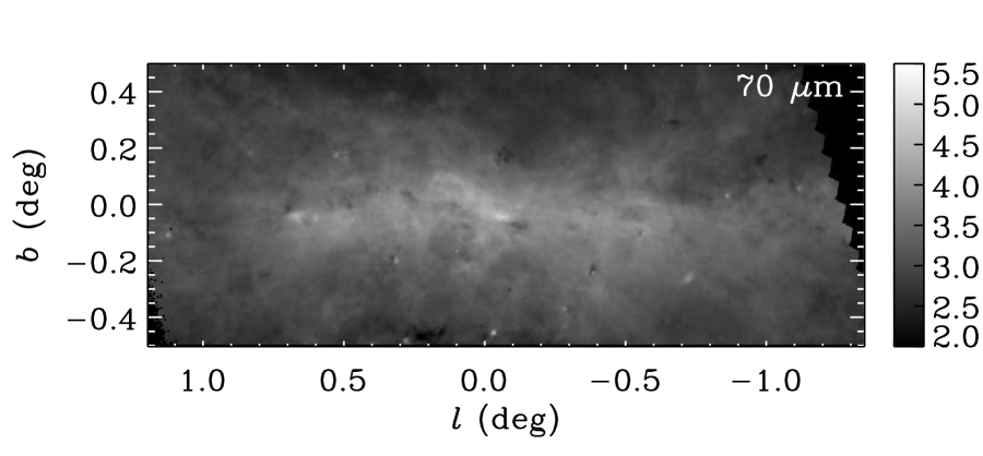
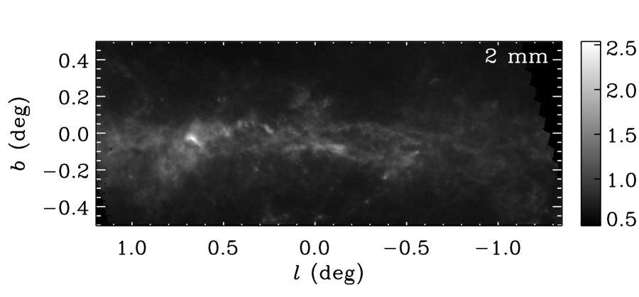
Figure 11: Images of 70 $\mu$m (top) and 2 mm (bottom) emission extrapolated from the fixed $\beta=2.25$ model of the 160–500 $\mu$m emission. The data are convolved to $37^{\prime\prime}$ resolution. These images are visually similar to the observed intensities shown in Figures 2 and 4, and are shown on the same logarithmic display ranges.

The observed 70 µm emission is always larger than the 70 µm intensity extrapolated from the model (Figure 12). The median ratio of the observed to predicted intensities is 2.1. The ratio tends to be higher in regions where the temperature is low, even though such regions can be optically thick at 70 $\mu$m and appear as IR dark clouds. The underestimate is likely due to two factors. The first is the neglect of a distribution of dust temperatures in the model. Warmer dust (either smaller dust and/or stochastically heated dust) will add intensity at the shorter wavelengths, broadening the spectrum. The second factor is the adoption of $\beta=2.25$, which leads to a more sharply peaked spectrum than flatter values of the emissivity index. While the steep index is found to fit the longer wavelengths, it is not necessary that this index continues to apply at shorter wavelengths. In either case, a more complete and physical model of the ISM emission would require additional parameters to fit the 70 µm data. However at 160 – 500 µm wavelengths, the fit is already sufficiently good that additional parameters are not statistically warranted.

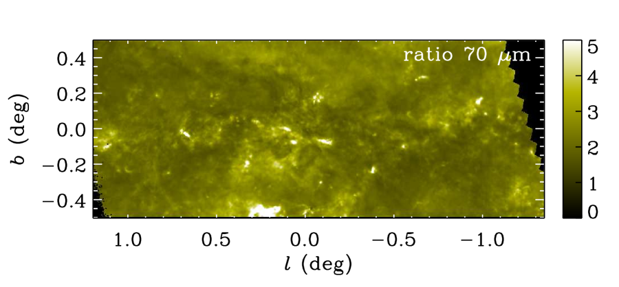
Figure 12: Ratio of observed to extrapolated 70 µm intensities (from Figures 2 and 11). The linear grayscale range is [0,5]. White regions, where the observed 70 $\mu$m intensity is significantly greater than the extrapolated intensity, include star-forming regions with warm dust and, prominently, cold molecular clouds and IRDCs.

Despite the steep emissivity index, the model generally overestimates the 2 mm emission, especially in the cold dense molecular clouds of Sgr B2 and the Galactic center (Figure 13). However, there are many structures where the observed 2 mm emission is in excess of the extrapolated dust emission. These include: extended and compact regions in Sgr B2, and Sgr B1; the Arches, Sickle, and Pistol Nebula; The Sgr A region; and other regions near Sgr C. Additionally, the brightest of the nonthermal filaments in the Galactic center is also evident, especially to the south of the Sickle nebula. There is very weak evidence of emission from some of the other adjacent parallel filaments. However, none of the other nonthermal filaments are detected at other locations around the Galactic center.

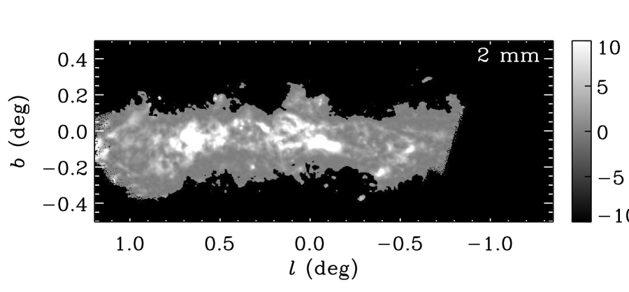
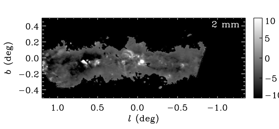
Figure 13: The observed 2 mm intensity (top) displayed on a linear grayscale range of [-10,10] MJy sr^-1, and the difference (bottom) between the observed and extrapolated 2 mm intensities on the same display range ($37^{\prime\prime}$ resolution). The difference image shows that most of the 2 mm emission is associated with thermal emission from dust. In regions where $T_{\rm d}$ is low, the emission is sometimes over-subtracted (appearing dark). Regions exhibiting 2 mm emission in excess of the dust emission (bright in the difference image) are H II regions and ionized structures that radiate via free-free emission at radio wavelengths, and non-thermal emission from the central filament of the Galactic center Radio Arc.

4 Discussion

The far-IR spectral index of $\beta=2.25$ derived here is steeper than would be expected for typical carbon grains ($\beta=1$) or silicate grains ($\beta=2$). However the relatively high value of $\beta$ is similar to that derived in other studies that fit for dust properties in selected areas or over the whole sky. For example, Planck Collaboration et al. (2014) used Planck observations at $30^{\prime}$ resolution to fit dust emission over the whole sky. They found $\beta\approx 1.6$ at high Galactic latitudes ($|b|\gtrsim 10\arcdeg$), but increasing to $\beta=1.8-2.0$ in the inner Galactic plane ($|l|\lesssim 30$). Using 450 and 850 $\mu$m SCUBA observations of the CMZ combined with 100 $\mu$m IRAS data, Pierce-Price et al. (2000) found vales of $\beta\sim 2.4$ when $\beta$ was allowed to be a free parameter of their model. Paradis et al. (2010) used Herschel data at 160, 250, 350, and 500 $\mu$m, and IRAS (IRIS) 100 $\mu$m data (Miville-Deschênes & Lagache, 2005) to model dust in two fields at $l=30\arcdeg$ and $l=59\arcdeg$. Their derived results at $l=30\arcdeg$ have a similar mean $T_{\rm d}$ and $\beta$ as ours, but show a much stronger inverse correlation between these two parameters. The lack of correlation towards the Galactic center may be caused by more intrinsic variation in dust properties along longer lines of sight. The lack of spatial smoothness in the derived $T_{\rm d}$ and $\beta$ (Fig. 5), and the sometimes spurious results, may be the response to noise in the data when using $\chi^{2}$ fitting methods (Juvela & Ysard, 2012; Juvela et al., 2013).

The total dust masses within the 0.04, 0.08, and 0.3  $M_{\sun}$ asec^-2 contours shown in Figure 8 are 4.3, 3.5, and $0.99\times 10^{5}$ $M_{\sun}$ when 0.04 $M_{\sun}$ asec^-2 is subtracted as background. With no background subtraction, the dust masses are 7.8, 4.6, and $1.05\times 10^{5}$ $M_{\sun}$, and the total dust mass in the shown image is $1.3\times 10^{6}$ $M_{\sun}$. Integrating the dust mass within the 0.08 $M_{\sun}$ asec^-2 contour and where $0.75>l>-0.65$ yields $2.4\times 10^{5}$ $M_{\sun}$ over an area of $4.2\times 10^{-5}$ sr [consistent with the area and the $3\times 10^{7}$ $M_{\sun}$ gas mass reported for the twisted ring structure by Molinari et al. (2011)].

It was expected that extrapolation of the single-temperature dust model to 70 $\mu$m would underestimate the emission in star-forming regions where warm dust is common. This is indeed found in our modeling. However, underestimates also are unexpectedly found at the locations of IRDCs and other low temperature regions (Figure 12). This result indicates that the 70 $\mu$m emission is coming from a substantially warmer dust component, possibly smaller or stochastically heated grains, or from warmer dust along the line of sight.

The extrapolation of the model to 2 mm shows that the observed emission can be brighter or fainter than the model prediction (Figure 13). The model tends to over-predict emission in the giant molecular clouds of Sgr B2, and the twisted ring of molecular clouds (Molinari et al., 2011). These are also well-correlated with regions of low dust temperature, suggesting a value of $\beta>2.25$ would be applicable to the colder clouds. This is weakly evident in the initial model which allowed a freely varying $\beta$, but is obscured by the overall noisiness of that unconstrained model (Figs. 5, 7). An additional contribution to overestimates of the 2 mm emission may be caused by missing large-scale structure in the GISMO image (§2.1), although the small scale of some overestimated features indicates that this cannot be the sole explanation.

Finally, the real regions of interest are where there is 2 mm emission in excess of the model prediction. These regions are places where the 2 mm observations are sensitive to emission components other than the thermal emission from dust. For the most part, the excess regions correspond to the known star-forming regions and ionized structures in the Galactic center. The most prominent are Sgr A and its nearby H II regions Sgr A A-D (these 4 compact H II regions are not fully resolved from one another), the Arches, the Sickle and the Pistol Nebula, Sgr B1, and Sgr C. A large and bright region of excess emission is located around and to the south of the compact H II regions embedded in Sgr B2. Most surprisingly, there is excess 2 mm emission from the central filament of the Radio Arc. The emission extends southward from the vicinity of the Sickle and Pistol Star, $(l,b)=(0.16,-0.06)$, to a location near $(l,b)=(0.14,-0.21)$. The Radio Arc is the largest and brightest of the collection of non-thermal filaments that have been identified in the Galactic center. A detailed investigation of this feature and the 2 mm emission from other non-dust sources is presented by Staguhn et al. (2019, Paper II).

In H II regions, the dust emissivity, $\epsilon_{\nu}^{\rm{IR}}(\lambda)$, is given by

$$\epsilon_{\nu}^{\rm{IR}}(\lambda)=4n_{\rm d}\ m_{\rm d}\ \kappa(\lambda)\ \pi B_{\nu}(T_{\rm d},\lambda)$$ (7)

where $n_{\rm d}$ is the number density of dust grains, $m_{\rm d}$ is the mass of a single dust grain, $\kappa(\lambda)$ is the mass absorption coefficient for the dust, and $B_{\nu}(T_{\rm d},\lambda)$ is the Planck function evaluated at the dust temperature, $T_{\rm d}$. Meanwhile, the free-free emissivity, $\epsilon_{\nu}^{\rm{ff}}(\lambda)$, is given by:

$$\epsilon_{\nu}^{\rm{ff}}(\lambda)=C\ g_{\rm ff}\ \frac{n_{\rm e}\ n_{\rm i}}{T^{0.5}\ e^{h\nu/kT}}$$ (8)

where $C$ is a numerical constant ($\approx 5.44\times 10^{-41}$), $g_{\rm ff}$ is the gaunt factor, $n_{\rm e}$ and $n_{\rm i}$ are the number densities of electrons and ions, and $T$ is the gas temperature. Thus for a dusty region of ionized gas, the observed ratio, $R$, of 70 $\mu$m emission from $T_{\rm d}=51$ K dust (Kaneda et al., 2012) to 2 mm free-free emission from $T=10^{4}$ K gas can be used a rough diagnostic of the electron density via

$$R\approx 1.7\times 10^{6}\ n_{\rm e}^{-1}$$ (9)

assuming a dust-to-gas mass ratio of $Z=0.01$. If the gas temperature were instead taken to be 8000 K, then the electron density derived from the ratio of IR to free-free emission would increase by $\sim 10\%$. The coefficient in Equation 9 is much more sensitive to $T_{d}$, dropping by a factor of $\sim 70$ if $T_{d}=25$ K.

To employ this relation as a density diagnostic, we have plotted the 2 mm free-free emission (i.e. the residual after subtraction of the ISM dust contribution), against the 70 $\mu$m emission in Figure 14. We compare with the observed 70 $\mu$m emission, and with the emission after the subtraction of the extrapolated emission of cold dust component determined from the 160-500 $\mu$m observations. The subtraction of this colder dust component is intended to better isolate the warmer emission from H II regions which produce the free-free emission. The comparison is limited to regions where $I_{\nu}(70\mu{\rm m})>10^{4}$ MJy sr^-1, and where the residual $I_{\nu}(2{\rm mm})>0$ MJy sr^-1 after adjustment for the (negative) median background level. These scatter plots are shaded as a function of $n_{\rm e}$ as indicated by the diagonal lines. Figure 15 maps out the locations of the points in Figure 14 using the same color coding for the density $n_{\rm e}$. Without subtraction of the cold dust contribution at 70 $\mu$m, the relatively small variation in the selected 70 $\mu$m data means that the implied density is largely determined by the residual 2 mm brightness. For example the extremely bright regions in Sgr B2 imply the highest densities. The less bright regions at Sgr B1, the Arches, and Sgr A have somewhat lower implied densities. If the extrapolated emission of the colder dust is subtracted from the 70 $\mu$m emission, the implied densities near Sgr B2 and Sgr A remain high, with a slight increase. Implied densities are more strongly increased for the fainter regions, which still exhibit large-scale structure though the structure is no longer directly correlated with the observed intensity.

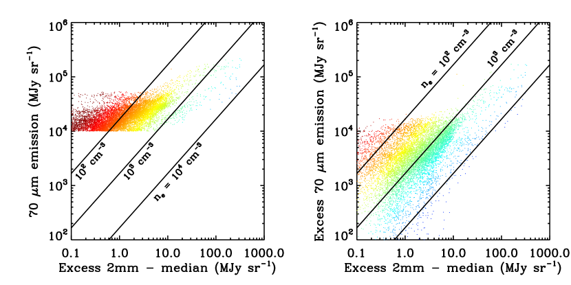
Figure 14: Ratio of residual 2 mm emission (mostly free-free) to 70 $\mu$m emission without (left) and with (right) subtraction of the emission of cold dust extrapolated from longer wavelengths. The points are shaded as a function of $n_{\rm e}$, with several lines of constant density overplotted for guidance.

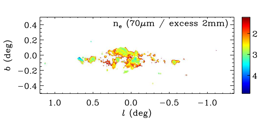
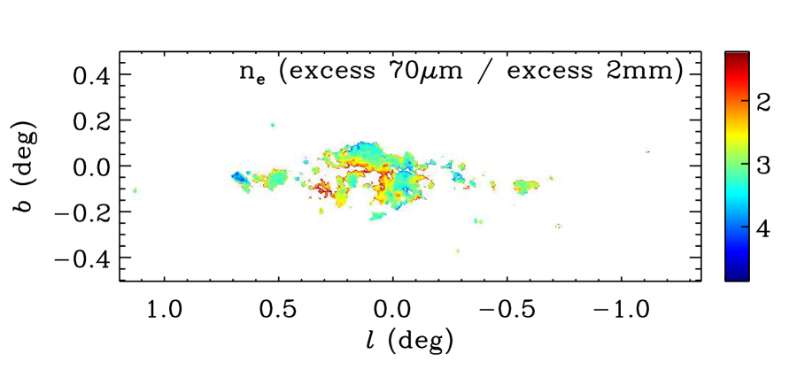
Figure 15: Maps of the logarithm of the electron density, $\log(n_{\rm e})$, implied by the ratio of residual 2 mm emission (mostly free-free) to 70 $\mu$m emission without (top) and with (bottom) subtraction of the emission of cold dust extrapolated from longer wavelengths. The latter case better isolates dust emission from warm regions where free-free emission is more likely to arise, and results in derived $n_{\rm e}$ values that are less correlated with the 70 $\mu$m brightness. The color scale for $\log(n_{\rm e})$ is the same as in Figure 14.

Electron densities are more typically estimated from the ratios of ground state fine structure lines. Such determinations may be affected by extinction effects, but are only very weakly dependent on the gas temperature. Rodríguez-Fernández & Martín-Pintado (2005) derived $n_{\rm e}<30-200$ cm^-3 from the [O III] 25/88 $\mu$m line ratios observed with ISO in several lines of sight in the CMZ. Simpson et al. (2018) used the FIFI-LS instrument on SOFIA to observe this line ratio in the Sgr B1 region, finding $n_{\rm e}\sim 300$ cm^-3, with some denser regions along some edges of Sgr B1. Using Spitzer observations of [S III] 18.7/33.5 $\mu$m line ratios, Simpson (2018) typically found $n_{\rm e}\sim 300$ cm^-3 in large regions across the CMZ, and $n_{\rm e}\sim 300-600$ cm^-3 across the Arches region in particular (Simpson et al., 2007). Direct comparison with the Arches results shows our densities are higher by factors of 1-10. Better agreement could be achieved by adjusting the estimates of one or more of the parameters in Equations (7) or (8), but without further information it is impossible to judge which of the parameters should be adjusted.

5 Summary

GISMO 2 mm observations of the Galactic center are dominated by the thermal emission of dust in the general ISM and particularly in molecular clouds. We model the far-IR emission seen by Herschel in order to predict and remove dust emission from the 2 mm image. The dust temperature varies about a mean value of $T_{\rm d}\approx 19$ K. Even though we find and set a relatively steep spectral index for the dust emission, $\beta=2.25$, the 2 mm emission extrapolated from shorter-wavelength measurements is often overestimated for cold molecular clouds. This is consistent with previous studies finding an inverse correlation between spectral index and dust temperature. Star-forming regions and other ionized structures show additional 2 mm emission arising from the free-free mechanism. Nonthermal emission from the central filament of the Galactic center Radio Arc is also detected at 2 mm. This is the shortest wavelength at which this feature has been detected.

References

- Abuter et al. (2019) Abuter, R., Amorim, A., Bauboeck, M., et al. 2019, arXiv e-prints, arXiv:1904.05721
- Aniano et al. (2011) Aniano, G., Draine, B. T., Gordon, K. D., & Sandstrom, K. 2011, PASP, 123, 1218
- Baars et al. (1987) Baars, J. W. M., Hooghoudt, B. G., Mezger, P. G., & de Jonge, M. J. 1987, A&A, 175, 319
- Bally et al. (2010) Bally, J., Aguirre, J., Battersby, C., et al. 2010, ApJ, 721, 137
- Cotera et al. (2005) Cotera, A. S., Colgan, S. W. J., Simpson, J. P., & Rubin, R. H. 2005, ApJ, 622, 333
- Culverhouse et al. (2010) Culverhouse, T., Ade, P., Bock, J., et al. 2010, ApJ, 722, 1057
- Figer et al. (1999) Figer, D. F., McLean, I. S., & Morris, M. 1999, ApJ, 514, 202
- Figer et al. (2002) Figer, D. F., Najarro, F., Gilmore, D., et al. 2002, ApJ, 581, 258
- Genzel et al. (2003) Genzel, R., Schödel, R., Ott, T., et al. 2003, ApJ, 594, 812
- Ginsburg et al. (2013) Ginsburg, A., Glenn, J., Rosolowsky, E., et al. 2013, ApJS, 208, 14
- Griffin et al. (2010) Griffin, M. J., Abergel, A., Abreu, A., et al. 2010, A&A, 518, L3
- Juvela et al. (2013) Juvela, M., Montillaud, J., Ysard, N., & Lunttila, T. 2013, A&A, 556, A63
- Juvela & Ysard (2012) Juvela, M., & Ysard, N. 2012, A&A, 541, A33
- Kaneda et al. (2012) Kaneda, H., Yasuda, A., Onaka, T., et al. 2012, A&A, 543, A79
- Kovács (2008) Kovács, A. 2008, in Proc. SPIE, Vol. 7020, Millimeter and Submillimeter Detectors and Instrumentation for Astronomy IV, 70201S
- Landsman (1995) Landsman, W. B. 1995, in Astronomical Society of the Pacific Conference Series, Vol. 77, Astronomical Data Analysis Software and Systems IV, ed. R. A. Shaw, H. E. Payne, & J. J. E. Hayes, 437
- Miville-Deschênes & Lagache (2005) Miville-Deschênes, M.-A., & Lagache, G. 2005, ApJS, 157, 302
- Molinari et al. (2011) Molinari, S., Bally, J., Noriega-Crespo, A., et al. 2011, ApJ, 735, L33
- Molinari et al. (2016) Molinari, S., Schisano, E., Elia, D., et al. 2016, A&A, 591, A149
- Morris & Serabyn (1996) Morris, M., & Serabyn, E. 1996, ARA&A, 34, 645
- Paradis et al. (2010) Paradis, D., Veneziani, M., Noriega-Crespo, A., et al. 2010, A&A, 520, L8
- Pierce-Price et al. (2000) Pierce-Price, D., Richer, J. S., Greaves, J. S., et al. 2000, ApJ, 545, L121
- Planck Collaboration et al. (2014) Planck Collaboration, Abergel, A., Ade, P. A. R., et al. 2014, A&A, 571, A11
- Planck Collaboration et al. (2015) Planck Collaboration, Ade, P. A. R., Aghanim, N., et al. 2015, A&A, 580, A13
- Poglitsch et al. (2010) Poglitsch, A., Waelkens, C., Geis, N., et al. 2010, A&A, 518, L2
- Pound & Yusef-Zadeh (2018) Pound, M. W., & Yusef-Zadeh, F. 2018, MNRAS, 473, 2899
- Reich et al. (2000) Reich, W., Sofue, Y., & Matsuo, H. 2000, PASJ, 52, 355
- Rodríguez-Fernández & Martín-Pintado (2005) Rodríguez-Fernández, N. J., & Martín-Pintado, J. 2005, A&A, 429, 923
- Simpson (2018) Simpson, J. P. 2018, The Astrophysical Journal, 857, 59
- Simpson et al. (1997) Simpson, J. P., Colgan, S. W. J., Cotera, A. S., et al. 1997, ApJ, 487, 689
- Simpson et al. (2007) —. 2007, ApJ, 670, 1115
- Simpson et al. (2018) Simpson, J. P., Colgan, S. W. J., Cotera, A. S., Kaufman, M. J., & Stolovy, S. R. 2018, ApJ, 867, L13
- Staguhn et al. (2019) Staguhn, J., Arendt, R. G., Dwek, E., et al. 2019, ApJ, submitted
- Staguhn et al. (2008) Staguhn, J., Allen, C., Benford, D., et al. 2008, Journal of Low Temperature Physics, 151, 709
- Staguhn et al. (2006) Staguhn, J. G., Benford, D. J., Allen, C. A., et al. 2006, in Proc. SPIE, Vol. 6275, Society of Photo-Optical Instrumentation Engineers (SPIE) Conference Series, 62751D
- Wang et al. (2006) Wang, Q. D., Dong, H., & Lang, C. 2006, MNRAS, 371, 38
- Wang et al. (2002) Wang, Q. D., Lu, F., & Lang, C. C. 2002, ApJ, 581, 1148
- Yusef-Zadeh et al. (2015) Yusef-Zadeh, F., Bushouse, H., Schödel, R., et al. 2015, ApJ, 809, 10
- Yusef-Zadeh et al. (2009) Yusef-Zadeh, F., Hewitt, J. W., Arendt, R. G., et al. 2009, ApJ, 702, 178