Synchronous Maneuver Searching and Trajectory
Planning for Autonomous Vehicles in Dynamic Traffic Environments

Abstract

10For1 [] 10In1In [] the real-time decision-making and local planning process of autonomous vehicles in dynamic environments, the autonomous driving system may fail to find a reasonable policy or even gets trapped in some situation due to the complexity of global tasks and the incompatibility between 10upper level1upper level [] maneuver decisions with the10low-level1 [] 10lower level1lower level [] trajectory planning. To solve this problem, this paper presents a synchronous maneuver searching and trajectory planning (SMSTP) algorithm based on the topological concept of homotopy. Firstly, a set of alternative maneuvers with boundary limits are enumerated on a multi-lane road. Instead of sampling numerous paths in the whole spatio-temporal space, we, for the first time, propose using Trajectory Profiles (TPs) to quickly construct the topological maneuvers represented by different routes, and put forward a corridor generation algorithm based on graph-search. The bounded corridor further constrains the maneuver’s space in the spatial space. A step-wise heuristic optimization algorithm is then proposed to synchronously generate a feasible trajectory for each maneuver. To achieve real-time performance, we initialize the states to be optimized with the boundary constraints of maneuvers, and we set some heuristic states as terminal targets in the quadratic cost function. The solution of a feasible trajectory is always guaranteed only if a specific maneuver is given. The simulation and realistic driving-test experiments verified that the proposed SMSTP algorithm has a short computation time which is less than 37ms, and the experimental results showed the validity and effectiveness of the SMSTP algorithm.

I Introduction

Autonomous driving has been extensively studied in the past three decades and has a wide variety of applications, especially in intelligent transportation systems. However, the thriving of autonomous driving does not give birth to a sufficiently-developed pilot system. There are still many research challenges in developing autonomous driving systems in complex environments. Among these challenges, real-time maneuver decision and local planning are two key technologies for dealing with dynamic traffic. Generally, a typical hierarchical maneuver reasoning and trajectory planning system is applied in most autonomous vehicles [buehler2009DARPAUrbanChallengea]. The hierarchical design can result in inconsistent situations. The upper10layer1 [] 10level1level [] of maneuver reasoning does not guarantee a favourable space for the lower10layer1 [] 10level1level [] of trajectory planning. Besides, maneuver reasoning in only spatial space or in spatio-temporal space with a short horizon does not discover more reasonable maneuvers, especially in the scenarios of lane merging, turning at intersections, etc. In the maneuver decision10layer1 [] 10level,1level, [] various drive strategies are decided according to global task (e.g. speed limit, intersection precedence handling), and local traffic (e.g. surrounding vehicles, obstacles in lane). Traditionally, the rule-based finite state machine [montemerlo2009JuniorStanfordEntry] and decision trees [Miller2008Team] have been widely used for 10the1the [] maneuver decision. The experience-based rules can reliably deal with deterministic and rather simple traffic situations well, but it generalizes poorly to unknown situations. The problem lies in that the artificial rules is not robust and completeness are not guaranteed. At the same time, machine learning based decision methods also have been investigated elaborately [Bahram2016AGame, lenz2016TacticalCooperativePlanning, li2017GameTheoreticModeling, talebpourModelingLaneChangingBehavior2015]. These methods model the interactions between the agent and other traffic participants in discrete actions and search an optimal action in a tree graph. Although these methods have developed traditional rules in some specific traffic situations, they still rely on artificially designed states or hand-crafted feature sets, and sometimes have problems with oscillatory behaviours and integrate the traffic rules poorly.

For the lower10layer1 [] 10level1level [] of trajectory planning, given a certain maneuver, it searches a set of executable trajectories connecting the start state space to target state space independently[johnson2012Optimal]. David et al. [gonzalez2015A] have surveyed several methods of trajectory planners for autonomous vehicles, which will not be repeated here. A hierarchical pilot system may fail in tough situations, since the conservative maneuver decision can hardly guarantee enough space to plan a safe and comfort trajectory. A reasonable pilot system requires that the trajectory planner should distinguish between maneuvers and the maneuver-decision maker should guarantee a feasible trajectory at the same time.

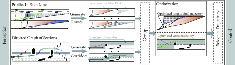
Figure 1: System architecture of SMSTP algorithm.

Apparently, a close integration of 10the1the [] maneuver decision and trajectory planning requires that all feasible tunnels should be extracted from the whole spatio-temporal space. Similarly, human drivers find a desired tunnel with a quick glance at the surrounding environments. Chen [chen2005TopologicalApproachPerceptual] indicates that the global topological perception is prior to the perception of other geometrical properties. In other words, the topological perception based on physical connectivity emerges earlier than the geometric perception. The topological perception occurs in only five milliseconds at the early stages of visual perception, and this explains why human drivers are talented in making decision10s.1s. [] Taking the lane change, for example, a lane change can be divided into mandatory lane change (occurs when a vehicle must get into the target lane in limited time or space) and discretionary lane change (maintains high cruise speed in natural traffic flow). Obviously, a lane change involves a dichotomy between the endogenously generated signals (e.g. traffic rules, drive styles or the motivation) and physical stimuli (e.g. lane boundaries, static obstacles and dynamic objects)[bisley2010AttentionIntentionPriority]. The combined dichotomy determines task-level expectation of a driver whilst the physical stimuli decide the topological perception that is, the tunnels in the spatio-temporal space. Inspired by this, we mainly focus on maneuver searching based on the topological tunnels in this paper.

Currently, two main topology-based methods have been extensively investigated, namely, the sampling based methods and the combinatorial methods. Sampling based methods group paths laterally shifted from a lane-center with motion primitives smoothly connected [gu2016AutomatedTacticalManeuver, gu2017ImprovedTrajectoryPlanning, sontges2018ComputingDrivableArea]. The maneuvers are10defined1 [] 10generated1generated [] by clustering paths into the same groups or homotopy classes. The discrete sampling sacrifices optimality and the fixed look-ahead time will prevent the algorithm from finding more smoother maneuvers. In addition, sample-based methods have problems 10in1in [] dealing traffic rules where precedence or other semantic elements must be considered. The second kind is the combinatorial method using a divide-and-conquer strategy. Firstly, different convex decomposition methods, such as cell decomposition and reference-frame methods are utilized to enumerate different homotopy classes in the unstructured environments [Bes2012Path, bhattacharya2012TopologicalConstraintsSearchbased, bhattacharya2015PersistentHomologyPath, kuderer2014OnlineGenerationHomotopicallya, rosmann2017IntegratedOnlineTrajectorya], then suboptimal paths are generated in each homotopy class. The idea of generating distinct topologies first of all, has also been used for on-road situation [zhan2017SpatiallypartitionedEnvironmental, park2015HomotopyBasedDivideandConquerStrategy, bender2015CombinatorialAspectMotiona]. Bender et al.[bender2015CombinatorialAspectMotiona] distinguish different maneuvers according to surrounding dynamic vehicles. However, these methods are merely applicable to quasi-static traffic situations. Florent et al.[altche2017PartitioningFreeSpacetime] extend the planning problem into 3D space by partitioning the collision-free space in discrete time, which results in a graph method for a deep path search with only one path generated. Then, the trajectory generation problem is solved in decomposed non-convex space by using quadratic optimizing approach. Moreover, the optimization sometimes finishes without a feasible solution. In contrast to the proposed SMSTP algorithm, these methods have two main disadvantages in dealing with on-road traffic. To the authors's knowledge, the first disadvantage is that current methods aim at finding out only one optimal trajectory either by sampling in the spatio-temporal space, or by solving a non-convex optimization problem. Even if these methods find only one optimal solution, they require either heavy computation load or excessive time for a real-time system respectively. The other is that these methods do focus on the optimal trajectory. However, to deal with the complex traffic, the expectation and preference of passengers vary at different situations thus leading to a discrete changing of the cost function. Only one optimal solution to a specific cost function cannot deal with situations where multiple alternative policies are needed.

The main difficulty of optimization-based method lies in that generating a good initialization of the solution is never easy. Apart from that, focusing on a global optimal trajectory tends to face a dilemma in many circumstances. The optimum refers to the best solution under given conditions with respect to a quadratic cost function. Nevertheless, the maneuver searching and trajectory planning problem for autonomous vehicles cannot be represented in a single cost function. The reason is that the maneuver decision is discrete, and the cost function varies in different traffic environments and long short-term expectations. In addition, optimum requires a huge cost for computational time and space for a real-time system. Nevertheless, sometimes a solution is not guaranteed. As a matter of fact, a feasible and comfort trajectory satisfies the expectation of most people in regular driving circumstances. Thus, instead of searching a global optimal trajectory, we focus on finding out a group of alternative solutions in different maneuvers each of which has a smooth trajectory.

In this work, a novel synchronous maneuver searching and trajectory planning (SMSTP) algorithm is proposed based on the topological concept of homotopy, whose overall architecture is shown in Fig.1 The key contributions are two-folds. Firstly, we propose a topological maneuver searching method by partitioning the spatio-temporal space10in1 [] 10into1into [] two 2D planes and reassembling the matched corridors and routes in each plane. We come up with TPs in adjacent $s$–$t$ planes for the first time to represent a topological route. A TP is a profile combining different segments of vehicles' trajectories in the $s$–$t$ plane. A TP reveals a compact space that a series of trajectory points can locate in. By using TPs to represent a homotopy route, SMSTP avoids sampling discretely in the temporal dimension and gets a closed space for path planning without any collision area inside. In addition, we propose an effective corridor generation algorithm by searching a tree structure. The corridors constrain the lateral width of the maneuvers in the $d$–$s$ plane. Different from traditional methods using fixed sampling distance, our method faithfully splits the bands laterally shifted from the lane-center into sections according to the distribution of obstacles. Finally, the combination of routes and corridors10results in the topological maneuver1 [] 10gives birth to the topological maneuvers.1gives birth to the topological maneuvers. []

Secondly, we present a step-wise numerical optimization method to generate a smooth trajectory. The algorithm uses adjusted weights of cost10term1 [] 10functions1functions [] to balance the solution and constraints for longitudinal and lateral10optimization1 [] 10optimizations1optimizations [] successively, where the boundary constraints of a maneuver are given as initial values and a heuristic state is set as the terminal target while optimizing. Thus, the massive computational time cost for non-convex optimization is avoided. The proposed algorithm is validated in simulation and real traffic. The realistic experimental test results show the rapidity and adaptability of the SMSTP algorithm to various dynamic traffic.

10Note that the SMSTP algorithm cannot be directly used in urban traffic. The complex intersections and sharp turns require a whole picture of surrounding roads, thus the HD (High definition) map and the road topology are required. Given these prerequisites, the SMSTP algorithm can be used in complex environments.1Note that the SMSTP algorithm cannot be directly used in urban traffic. The complex intersections and sharp turns require a whole picture of surrounding roads, thus the HD (High definition) map and the road topology are required. Given these prerequisites, the SMSTP algorithm can be used in complex environments. []

The remainder of this paper is organized as follows. Section II introduces basic problem definitions. Section III presents the algorithm of generating different topological corridors and routes in detail. Section LABEL:sec_trajectory_optimizaiont describes the numerical optimization method for10our1 [] trajectory generation. Section LABEL:sec_exp gives the experiments of both simulation and driving test results to evaluate the proposed algorithm. Finally, Section LABEL:sec_conclusion concludes this paper.

II Problem Definition

II-A Notations

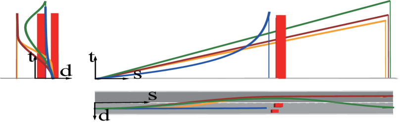
(a) 10Three orthographic views of the trajectories in Fig.1Three orthographic views of the trajectories in Fig. [] 2(b)

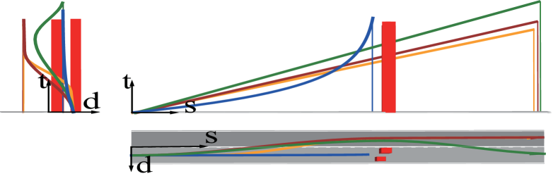
(b) 10Global view of right lane totally blocked. Three homotopy paths exist.1Global view of right lane totally blocked. Three homotopy paths exist. []

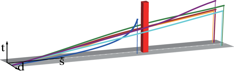
(c) 10Global view of right lane partly blocked. Five homotopy paths exist.1Global view of right lane partly blocked. Five homotopy paths exist. []

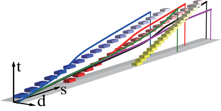
(d) 10Homotopy paths in traffic flow(boxes with the same gradient colors represent the same vehicle at different times).1Homotopy paths in traffic flow(boxes with the same gradient colors represent the same vehicle at different times). []

Figure 2: 10Homotopy paths in different scenarios. The long red boxes represent static obstacles. The orange and yellow trajectories belong to the same homotopy path. The trajectories in other colors represent different homotopy paths separately. $d$–$s$ is the Curvilinear coordinate. $s$–axis is tangent to the lane line, $d$–axis is orthogonal to $s$–axis. $t$–axis representing time is orthogonal to $d$–$s$ plane.1Homotopy paths in different scenarios. The long red boxes represent static obstacles. The orange and yellow trajectories belong to the same homotopy path. The trajectories in other colors represent different homotopy paths separately. $d$–$s$ is the Curvilinear coordinate. $s$–axis is tangent to the lane line, $d$–axis is orthogonal to $s$–axis. $t$–axis representing time is orthogonal to $d$–$s$ plane. []

II-A1 Planning Space

As shown in Fig.2, the lane lines are boundary constraints on a vehicle, and the spaces occupied by obstacles and vehicles are the collision10-free1 [] areas. The obstacles, the vehicles and the ego agent refer to the stationary entities, the moving traffic participants and the agent (ego autonomous vehicle) respectively in the following context without specific description. The obstacles will occupy the lane for all time. A vehicle in each lane covers either the whole lane (keeping in the lane) or two lanes (overtaking others, 10changing lane1changing lane [] ), and a vehicle moves along its trajectory in the 3D space (see Fig.2(d)). The number of the obstacles can be enormous. For the convenience of computation, a cost-map, $m_{cost}$ is generated from the obstacles. The side-ward boundaries are limited by lane lines $L_{lines}$. The state of a vehicle or the agent at time $t$ is given as $\mathbf{x}_{i}^{t}=[s_{i}^{t},d_{i}^{t},v_{i}^{t}]^{\top}$, which consists of the longitudinal and lateral positions $s_{i}^{t}$ and $d_{i}^{t}$ in the curvilinear-coordinate [chu2012LocalPathPlanninga] and the velocity $v_{i}^{t}$. $\mathbf{x}_{i}=[x_{0},...,x_{T}]^{\top}$ is the trajectory of a vehicle $i$ and $\mathbf{x}_{e}$ is the planned trajectory of the ego agent. For simplicity, $\mathbf{X}=\{x_{1},\dots,x_{M}\}$ is the set of trajectories with all other traffic participants, and $M$ is the number of vehicles.

II-A2 Corrdinates Conversion

As the lane lines are not always straight, various shapes of lane make it difficult to model lane structure in a unified form. Traditional methods use polynomial curves, splines, parabolic curves, etc [narote2018ReviewRecentAdvances] to fit a line, where the resultant curves are only precise within a short range and various models must be used to cover different road shapes. Instead of fitting curves, the lanes are represented by a line that is in a set of points with fixed interval. An accumulated reference path is used to convert between Curvilinear coordinate and Cartesian coordinate as shown in Fig.3. The reference path accumulates along a lane line. The reference path includes the pose $(x,y)$ in Cartesian coordinate, the perpendicular vector $\mathbf{d}_{n}$, the accumulated distance $s$ in Curvilinear coordinate and the curvature $\rho$ of each point. For conversion 10of any point $P$1of any point $P$ [] from $(x_{p},y_{p})$ to $(\bar{s}_{p},\bar{d}_{p})$, it searches the closest point on the reference path by binary search(this is guaranteed by a fixed interval of points in reference path)10.1 [] 10,1, [] and the accumulated distance is $\bar{s}_{p}$10,1 [] 10.1. [] 10the1 [] 10The1The [] lateral shift $\bar{d}_{p}$ is calculated by the point-to-line distance. For conversion 10of the point $P$1of the point $P$ [] from $(\bar{s}_{p},\bar{d}_{p})$ to $(x_{p},y_{p})$, it searches the accumulated length of $\bar{s}_{p}$ by binary search in reference path, and a shift 10$\bar{d}_{p}$1$\bar{d}_{p}$ [] from the corresponding point in $\mathbf{d}_{n}$ gets $(x_{p},y_{p})$. Apparently, the pose of10the agent1 [] 10ego vehicle1ego vehicle [] is10$(s_{ego},d_{ego})$1 [] 10$(s_{e},d_{e})$1$(s_{e},d_{e})$ [] in Curvilinear coordinate and is $(0,0)$ in local Cartesian coordinate.10And1 [] 10For1For [] conversions of other points related to vehicle, it only needs a shift to the coordinate of the10agent1 [] 10vehicle's1vehicle's [] pose.

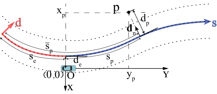
Figure 3: 10Conversions between two coordinates. The colored curve is the Curvilinear coordinate. XOY is the Cartesian coordinate of the ego vehicle.1Conversions between two coordinates. The colored curve is the Curvilinear coordinate. XOY is the Cartesian coordinate of the ego vehicle. []

II-B Homotopy Class

The utility of homotopy classes in vehicle navigation has been studied in [Bes2012Path]. A homotopy path class is defined as a set of paths that connect the start state and the terminal state in the same topology. Inspired by Bhattacharya's work [bhattacharya2012TopologicalConstraintsSearchbased], Gu [gu2016AutomatedTacticalManeuver] and Schulz [schulz2017EstimationCollectiveManeuvers] extended the co-terminal-guaranteed paths to spatio-temporal trajectory planning based on the idea of pseudo-homology where co-terminal is replaced by a co-region. Relaxing some specific end states to terminal regions has also been used in [zhan2017SpatiallypartitionedEnvironmental, altche2017PartitioningFreeSpacetime]. In this paper, lanes are distinguished as different topologies vividly, so the behavioral discovery is consistent with the road structure, i.e. the lane branches. Therefore, the top-level semantic instructions can be easily integrate into10a1 [] 10the1the [] maneuver decision.

For 10the1the [] maneuver decision, lanes should be considered in a discrete manner. As show in Fig.2(b), three homotopy paths exist when right (forward direction) lane is totally blocked by red obstacles. The brown and orange paths going to the end of the left lane are homotopic. The blue path goes straight and stops in front of obstacles. The green path leads the agent to the end of original lane with two lane-change avoiding the obstacles. When obstacles occupy part of the right lane in Fig.2(c), two more homotopy paths exist. One purple path goes to left lane after passing the obstacle on 10the1the [] right side. The other homotopy path leads the agent to the end of lane on 10the1the [] right 10side.1side. [] Paths derived from the discretization of lanes now are corresponding to different maneuvers topologically.

Considering the temporal aspect of vehicles, a different kind of homotopy paths exists in the spatio-temporal without collision with other vehicles. In Fig.2(d) two vehicles in the left lane yield three alternative collision-free spaces and the yellow vehicle splits right lane into two halves. Primitively, connecting the center of a vehicle at each time instance by a single line generates the future trajectory $\mathbf{x}$. A plane is expanded by $\mathbf{x}$ and10a line perpendicular to both $\mathbf{s}$ coordinate and $\mathbf{x}$1 [] 10$d$-axis.1$d$-axis. [] The plane splits spatio-temporal space into two halves. Each space is defined as a Trajectory Profile (TP), that is, a profile $P_{i}^{j}$ is the $j^{th}$ collision-free zone split by different vehicles without a hole in the $i^{th}$ lane, where $i$ and $j$ $\in$ {0, 1, 2, 3, …}. Fig.4 reappears the 3D view of TPs in Fig.2(d). The green profile $P_{0}^{0}$ is the space just behind the blue vehicle in the left lane, and the yellow profile $P_{1}^{1}$ is the space in front of the yellow vehicle. The purple trajectory taking over the red and the yellow vehicles successively arrives at the front region of the yellow vehicle. The corresponding maneuver can be represented by a sequence of connective profiles $\{P_{1}^{0}\rightarrow P_{0}^{2}\rightarrow P_{1}^{1}\}$, which means a unique homotopy class.

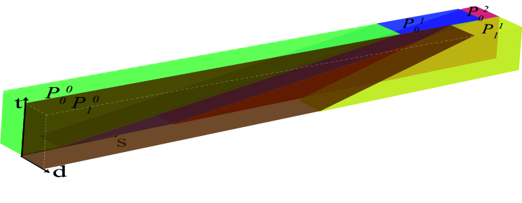
(a) 10The homotopy classes in global view.1The homotopy classes in global view. []

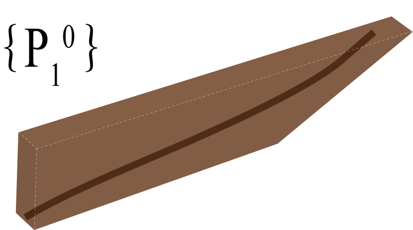
(b) 10Lane keep.1Lane keep. []

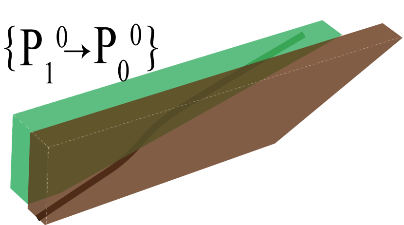
(c) 10To left.1To left. []

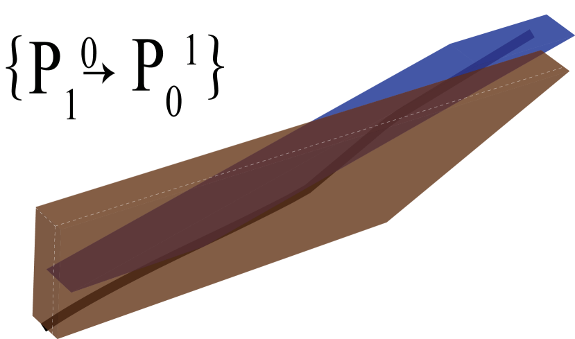
(d) 10To left.1To left. []

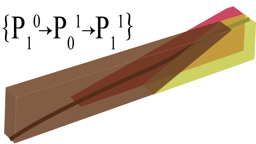
(e) 10Back after to left.1Back after to left. []

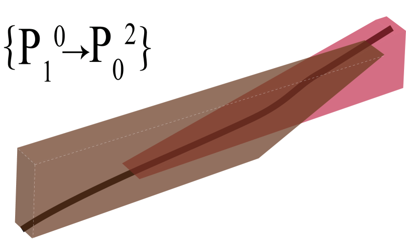
(f) 10To left.1To left. []

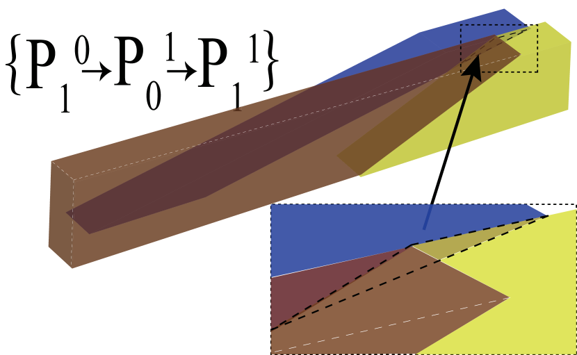
(g) 10Back after to left.1Back after to left. []

Figure 4: 10Homotopy classes consider temporal dimension. Profiles are created by the vehicles in Fig.1Homotopy classes consider temporal dimension. Profiles are created by the vehicles in Fig. [] 2(d). 10In Fig.1In Fig. [] 4(g)10, the time interval between profile $P_{0}^{1}$ and profile $P_{1}^{1}$ is too narrow to change to the right lane.1, the time interval between profile $P_{0}^{1}$ and profile $P_{1}^{1}$ is too narrow to change to the right lane. []

III Topology Generation

To enable an enumeration of maneuvers, a topological structure of the agent’s planning space must be generated. There are three basic steps needed. Firstly, we propose an algorithm of generating topological corridors by considering obstacles that limit the non-collision spatial space of the agent in the lanes. Then an algorithm of generating topological routes is presented using the mobility of our agent and future trajectories of other vehicles to split the whole spatio-temporal space. Finally, by matching the corridors and routes in lane level, we enumerate all possible maneuvers in the predicting horizon.

III-A Topology by Static Obstacles

As described in II-B, the agent has more choices to pass the occupied region when the obstacles block part of the lane. However, fewer options exist when the whole right lane is occupied in a double-lane road. The disordered and irregular obstacles give rise to the complexity of planning space. Firstly, the whole space are split into pieces, then, they are reconnected into several structured spaces where trajectory planning is easier.

III-A1 Lane Split and Reconnection

For being able to decide discretely on which side of a lane that the agent can go through, we split the lane into seven parallel bands based on experience. And the width of each band is $W_{b}=W_{lane}/7$, where $W_{lane}$ is the lane's width. Each band is bilaterally shifted from the10lane1 [] center 10of lane.1of lane. [] The center of middle band is the center of lane.10And1 [] The minimum width of drivable side $W_{d}$, is

$$W_{d}=\max(3W_{b},W_{vehicle}+2d_{safe})$$ (1)

where $d_{safe}$ is the safe distance to obstacles, and $W_{vehicle}$ is the width of a vehicle.

(a) Corridor 1.

(b) Corridor 2.

(c) Corridor 3.

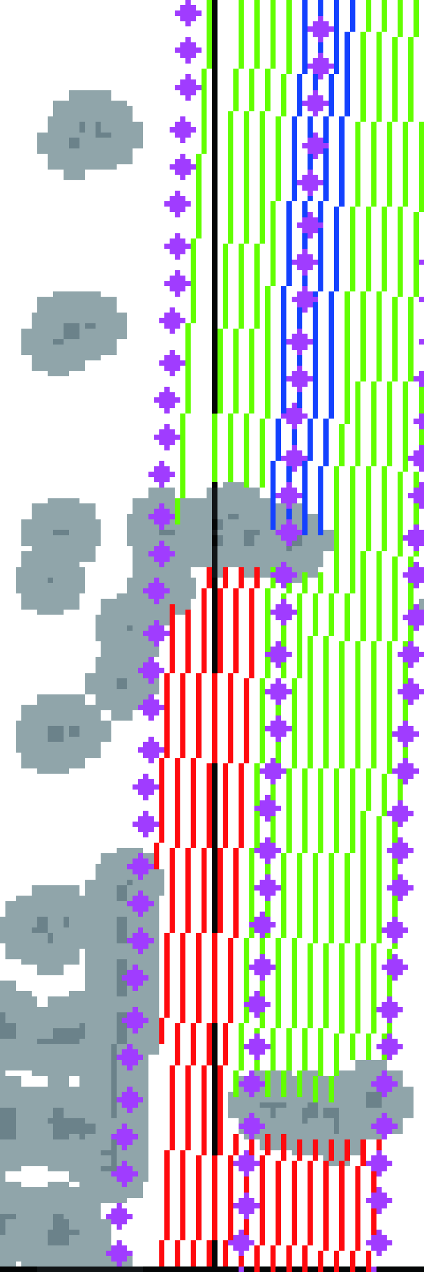
(d) Band split.

Figure 5: Homotopy paths in a double-lane road with obstacles. The red dots represent lane lines, and the blue dots represent left and right boundaries of a corridor. The colors of three sections in one band are red, cyan and blue respectively. 10The dark grey dots are the obstacles, and the light grey areas are the inflated area of obstacles.1The dark grey dots are the obstacles, and the light grey areas are the inflated area of obstacles. []

As shown in Fig.5, the obstacles occupy the lane permanently and cut one band into several sections. One section $s_{j\_k}^{i}$ is the $k_{th}$ section in $j_{th}$ band, and $i$ represents lane id. Where i $\in(0,1\dots N),j\in(0,1,\dots,7N)$ and $k\in(0,1,2)$.10Here at1 [] 10At1At [] most three sections in each band of N lanes are considered, since the smoothness of a lane is directly related to the distribution of the obstacles. An illustrative example is also shown in Fig.6, and the lane is split into five bands for the simplicity of explaining. Only the front two sections are enough to plan a reasonable path according to experience. The advantages are two folds. Firstly, the split is only related to the obstacles but not a designed sampling distance. The split implies a more natural choice of the sampling interval, thus avoiding an unevenness path from fixed value of sampling distance. Secondly, the number or the length of sections in one line directly reflects the smoothness of the front road, and this will guide the agent at what level the speed should be.

One generated section is viewed as a node while searching. One section connects only to those in adjacent bands. Given no more than three sections in each band, there are at most five edges connecting two bands. Sections are connected in a directed graph following rules 10below1below []

• The connection means that the adjacent sections have a minimum overlapping thresh (the width of the agent) along lane direction.

• Connections start from root section (where vehicle locates at) to the leftest and rightest sides separately.

• Different sections in the same line cannot connect to each other directly. The connection to different sections in one band has at least one transitional section in a adjacent line.

A directed graph of sections is generated once the connection work is done. The procedure is shown in Fig.6.

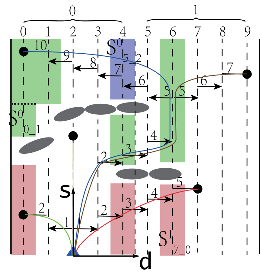
(a) Corridors starts in the left lane.

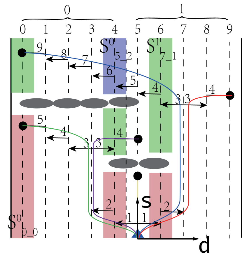
(b) Corridors starts in the right lane.

Figure 6: Terminal sections generated in two similar scenarios with different initial positions in two lanes. The start pose locates at the blue triangle. The grey areas are the inflated obstacles. The light red, cyan and blue bands are the corresponding sections in Fig.5. The arrow line with a number means the search direction with depth. The black dot at the end of each line represents a terminal section.

Algorithm 1 Generate Topological Corridors in 2D Space

1:cost-map:$m_{cost}$, lane lines:$L_{lines}$

2:corridors with different homotopy type:$C_{cor}$

3:$G_{sec}$ $\leftarrow$ generateSectionGraph($m_{cost},L_{lines}$)

4:$C_{sec}$ $\leftarrow$ generate-end-sections($G_{sec}$, $s_{r}$)

5:$C_{cor}$ $\leftarrow$ generate-Corridors($C_{sec},G_{sec}$)

6:

7:function generate-end-Sections($G_{sec}$, $s_{r}$)

8:    ${Init}$: unvisited sections $G_{uv}\leftarrow G_{sec}$, $C_{sec}\leftarrow s_{r}$

9:    while  $G_{uv}\neq\emptyset$  do

10:         for each  $s_{c}\in C_{sec}$ do $\triangleright$ $s_{c}$ is current section

11:             $s_{n}\leftarrow s_{n(i)}\cap s_{c}\neq\emptyset$, $i\subset[0,4]$

12:             $G_{uv}\leftarrow G_{uv}\backslash s_{c}$

13:             if  $s_{n}\neq\emptyset$  then

14:                 $G_{sec}\leftarrow G_{sec}\backslash s_{c}$

15:                 $G_{sec}\leftarrow G_{sec}\cup\{s_{n}\}$

16:             end if

17:         end for

18:    end while

19:    if  $s_{r}\notin G_{sec}$ then

20:         $G_{sec}\leftarrow G_{sec}\cup\{s_{r}\}$

21:    end if

22:    return $C_{sec}$

23:end function

24:

25:function generate-Corridors($C_{sec},G_{sec}$)

26:    ${Init}:$ Corridors:$C_{cor}\leftarrow\emptyset$

27:    for each  $s_{c}\in C_{sec}$ do

28:         if $s_{c}$ is much shorter than parent section  then

29:             $s_{c}\leftarrow s_{p}$ $\triangleright$ move to parent section

30:         end if

31:    end for

32:    for each  $s_{c}\in C_{sec}$ do

33:         $c_{cor}$ $\leftarrow$ connect from $s_{c}$ to $s_{r}$ $\triangleright$ get a corridor

34:         add $c_{cor}$ to $C_{cor}$

35:    end for

36:    for each  $c_{cor}\in C_{cor}$  do

37:         for each  $\bar{c}_{cor}\in C_{cor}{}\ \&\ c_{cor}\neq\bar{c}_{cor}$ do

38:             complement $c_{cor}$ with $c_{cor-next}$

39:         end for

40:         $c_{cor}\leftarrow$ smoothSectionInCorridor($c_{cor}$)

41:    end for

42:    return $C_{cor}$

43:end function

III-A2 Generate topological corridors in 2D space

Algorithm 1 shows high-level pseudo-code for the generation of topological corridors at each planning10circle1 [] 10cycle.1cycle. [] The directed graph of sections, $G_{sec}$, is created in line 3 given lane lines as bounds and a cost-map generated from obstacles. As shown in Fig.5 and 6, the connection between sections of adjacent lines is checked according to Rule 1.

One core function in line 4 finds the terminal sections of all possible topological corridors $C_{sec}$. Originally, the $C_{sec}$ is only initialized with root section $s_{r}$ (the blue triangle). The corridor searching starts from each element in $C_{sec}$ in every loop. If the current section $s_{c}$ in $C_{sec}$ connects to adjacent sections, then the connected sections are added into $C_{sec}$ for next loop quire and current section $s_{c}$ is removed (see line 7). Looping stops until all sections have been visited, and the elements left in $C_{sec}$ represent all potential topological corridors. Taking Fig.6(a), for example, searching starts with only root section $s_{2\_0}^{0}$ in $C_{sec}$. The next step confirms two connections that $s_{1\_0}^{0}$ and $s_{3\_0}^{0}$ are connected to $s_{2\_0}^{0}$, then $C_{sec}$ is updated with $s_{1\_0}^{0}$ and $s_{3\_0}^{0}$ instead of $s_{2\_0}^{0}$. In the next loop, $s_{0\_0}^{0}$ taking place of $s_{1\_0}^{0}$ becomes a real terminal section. Besides, unvisited sections $s_{4\_0}^{0}$ and $s_{4\_1}^{0}$ connect to $s_{3\_0}^{0}$ respectively and take place of $s_{3\_0}^{0}$ in $C_{sec}$. The search ends with four real terminal sections $s_{0\_0}^{0}$, $s_{7\_0}^{1}$, $s_{9\_0}^{1}$, $s_{0\_1}^{0}$ and one extra root section $s_{2\_0}^{0}$.

Procedure above mainly finds a possible path to the terminal section without left and right boundary constraints. The other core function in line 5 generates real drivable corridors. Due to the irregular shape and the complex distribution of the obstacles, some unreasonable corridors are inevitable. Illogical terminal sections are removed inside the first loop in line 27. The next loop body searches a corridor from terminal section to root section $s_{r}$ reversely. One problem still exists as the sections stretch from current position to either side, thus the corridor is unable to completely coverage a total lane. A quick solution is to query from sections of other corridors that connecting to either side of the current corridor. For this reason, corridors with missing part can be easily complemented. As illustrated in Fig.6(a), an incomplete corridor in red curve covers six sections in bands from 2 to 7. This corridor leads vehicle to Lane 1 before passing the obstacles and the uncovered sections of lane 1 can be complemented by querying from the corridor in brown curve that ends at $s_{9\_0}^{1}$. For the convenience to decide the width of corridor, some protuberant bands are truncated to fit adjacent bands. For example, the terminal section $s_{0\_1}^{0}$ in blue curve is trimmed off to match with parent section $s_{1\_1}^{0}$. Now all the drivable corridors are generated without considering the vehicles.

The corridor generation algorithm has three basic advantages as below. Firstly, the number and the length of sections are qualitative descriptions of the road smoothness. Secondly, the agent's position and obstacle distribution always implicitly ignore those corridors crossing more lateral bands. In Fig.6(b), a hidden corridor ($s_{5\_0}^{1}$$\rightarrow$$s_{3\_0}^{0}$$\rightarrow$$s_{6\_1}^{1}$$\rightarrow$$s_{0\_1}^{0}$) is ignored naturally, as the blue route reaches section $s_{6\_1}^{1}$ at third step firstly. And the hidden corridor is taken over since it takes10more1 [] 10a longer1a longer [