Probability distribution of the boundary local time
of reflected Brownian motion in Euclidean domains

Abstract

How long does a diffusing molecule spend in a close vicinity of a confining boundary or a catalytic surface? This quantity is determined by the boundary local time, which plays thus a crucial role in the description of various surface-mediated phenomena such as heterogeneous catalysis, permeation through semi-permeable membranes, or surface relaxation in nuclear magnetic resonance. In this paper, we obtain the probability distribution of the boundary local time in terms of the spectral properties of the Dirichlet-to-Neumann operator. We investigate the short-time and long-time asymptotic behaviors of this random variable for both bounded and unbounded domains. This analysis provides complementary insights onto the dynamics of diffusing molecules near partially reactive boundaries.

I Introduction

Diffusion in confined media is common for many physical, chemical and biological systems. The presence of reflecting obstacles or reactive surfaces drastically alters statistical properties of conventional Brownian motion and controls diffusion-influenced phenomena such as chemical reactions, surface relaxation or target search processes Redner ; Schuss ; Metzler ; Oshanin ; Bouchaud90 ; Grebenkov07 ; Benichou14 . A mathematical construction of such stochastic processes requires a substantial modification of the underlying stochastic equation. In fact, a specific term has to be introduced into the stochastic differential equation in order to ensure reflections and to prohibit crossing a reflecting boundary. In the simplest setting, the reflected Brownian motion $\bm{X}_{t}$ in a given Euclidean domain $\Omega\subset{\mathbb{R}}^{d}$ with a smooth enough boundary $\partial\Omega$ is constructed as the solution of the stochastic Skorokhod equation Ito ; Freidlin ; Anderson76 ; Brosamler76 ; Lions84 ; Saisho87 ; Hsu85 ; Williams87 :

$$d\bm{X}_{t}=\sigma\,d\bm{W}_{t}+\bm{n}(\bm{X}_{t}){\mathbb{I}}_{\partial\Omega}(\bm{X}_{t})d\ell_{t},\quad\bm{X}_{0}=\bm{x}_{0},$$ (1)

where $\bm{x}_{0}\in\bar{\Omega}=\Omega\cup\partial\Omega$ is a fixed starting point, $\bm{W}_{t}$ is the standard $d$-dimensional Wiener process, $\sigma>0$ is the volatility, $\bm{n}(\bm{x})$ is the normal unit vector at a boundary point $\bm{x}$, which is perpendicular to the boundary at $\bm{x}$ and oriented outwards the domain $\Omega$, ${\mathbb{I}}_{\partial\Omega}(\bm{x})$ is the indicator function of the boundary (i.e., ${\mathbb{I}}_{\partial\Omega}(\bm{x})=1$ if $\bm{x}\in\partial\Omega$, and $0$ otherwise), and $\ell_{t}$ (with $\ell_{0}=0$) is a nondecreasing process, which increases only when $\bm{X}_{t}\in\partial\Omega$, known as the boundary local time. The second term in Eq. (1), which is nonzero only on the boundary, ensures that Brownian motion is reflected in the perpendicular direction from the boundary. The peculiar feature of this construction is that the single Skorokhod equation determines simultaneously two tightly related stochastic processes: $\bm{X}_{t}$ and $\ell_{t}$. Even though $\ell_{t}$ is called local time, it has units of length, according to Eq. (1).

In physics literature, the reflected Brownian motion is often described without referring to the boundary local time $\ell_{t}$ by using the heat kernel (also known as the propagator), $G_{0}(\bm{x},t|\bm{x}_{0})$, which is the probability density of finding the process $\bm{X}_{t}$ at time $t$ in a vicinity of $\bm{x}\in\bar{\Omega}$, given that it was started from $\bm{x}_{0}\in\bar{\Omega}$ at time $0$. This heat kernel satisfies the diffusion equation

$$\partial_{t}G_{0}(\bm{x},t|\bm{x}_{0})=D\,\Delta_{\bm{x}}G_{0}(\bm{x},t|\bm{x}_{0})\qquad(\bm{x}\in\Omega),$$ (2)

where $D=\sigma^{2}/2$ is the diffusion coefficient of reflected Brownian motion, and $\Delta_{\bm{x}}$ is the Laplace operator acting on $\bm{x}$. This equation is completed by the initial condition $G_{0}(\bm{x},t=0|\bm{x}_{0})=\delta(\bm{x}-\bm{x}_{0})$ and Neumann boundary condition:

$$\partial_{n}G_{0}(\bm{x},t|\bm{x}_{0})=0\qquad(\bm{x}\in\partial\Omega),$$ (3)

where $\partial_{n}=(\bm{n}(\bm{x})\cdot\nabla)$ is the normal derivative and $\delta(\bm{x})$ is the Dirac distribution.

In turn, the boundary local time $\ell_{t}$ characterizes the behavior of reflected Brownian motion $\bm{X}_{t}$ on the boundary $\partial\Omega$ (Fig. 1). As first described by P. Lévy Levy , the boundary local time can be understood as the renormalized residence time of $\bm{X}_{t}$ in a thin layer near the boundary, $\partial\Omega_{a}=\{\bm{x}\in\Omega~{}:~{}|\bm{x}-\partial\Omega|<a\}$ up time $t$ Ito ; Freidlin ,

$$\ell_{t}=\lim\limits_{a\to 0}\frac{D}{a}\underbrace{\int\limits_{0}^{t}dt^{\prime}\,{\mathbb{I}}_{\partial\Omega_{a}}(\bm{X}_{t^{\prime}})}_{\textrm{residence time in}~{}\partial\Omega_{a}}.$$ (4)

This relation highlights that the residence time in the boundary layer $\partial\Omega_{a}$ vanishes in the limit $a\to 0$ when $\partial\Omega_{a}$ shrinks to the boundary $\partial\Omega$. This is not surprising given that the boundary $\partial\Omega$ has a lower dimension, $d-1$, as compared to the dimension $d$ of the domain $\Omega$, and the residence time on the boundary is strictly zero. In turn, the rescaling of the residence time in $\partial\Omega_{a}$ by the width $a$ of this layer yields a well-defined limit, namely, the boundary local time. Importantly, Eq. (4) implies that the residence time spent in a thin boundary layer $\partial\Omega_{a}$ can be approximated as $a\ell_{t}/D$, as soon as $a$ is small enough. The boundary local time $\ell_{t}$ is thus the proper intrinsic characteristics of reflected Brownian motion on the boundary, which is independent of the layer width used.

The boundary local time $\ell_{t}$ is also related to the number $\mathcal{N}_{t}^{a}$ of downcrossings of the boundary layer $\partial\Omega_{a}$ by reflected Brownian motion up to time $t$, multiplied by $a$, in the limit $a\to 0$ Ito ; Freidlin ,

$$\ell_{t}=\lim\limits_{a\to 0}a\,\mathcal{N}_{t}^{a}.$$ (5)

The number of downcrossings can be mathematically defined by introducing a sequence of interlacing hitting times $0\leq\delta_{0}^{(0)}<\delta_{0}^{(a)}<\delta_{1}^{(0)}<\delta_{1}^{(a)}<\ldots$ as

$$\delta_{n}^{(0)} =\inf\{t>\delta_{n-1}^{(a)}~{}:~{}\bm{X}_{t}\in\partial\Omega\},$$ (6a)

$$\delta_{n}^{(a)} =\inf\{t>\delta_{n}^{(0)}~{}:~{}\bm{X}_{t}\in\Gamma_{a}\},$$ (6b)

(with $\delta_{-1}^{(a)}=0$), where $\Gamma_{a}=\{\bm{x}\in\Omega~{}:~{}|\bm{x}-\partial\Omega|=a\}$. Here, one records the first moment $\delta_{0}^{(0)}$ when reflected Brownian motion hits the boundary $\partial\Omega$, then the first moment $\delta_{0}^{(a)}$ of leaving the thin layer $\partial\Omega_{a}$ through its inner boundary $\Gamma_{a}$, then the next moment $\delta_{1}^{(0)}$ of hitting the boundary $\partial\Omega$, and so on. In this setting, the number of downcrossings of the thin layer $\partial\Omega_{a}$ up to time $t$ (i.e., the number of excursions in the bulk) is the index $n$ of the largest hitting time $\delta_{n}^{(0)}$, which is below $t$:

$$\mathcal{N}_{t}^{a}=\sup\{n>0~{}:~{}\delta_{n}^{(0)}<t\}.$$

While the number of downcrossings diverges as $a\to 0$, its renormalization by $a$ yields a well-defined limit $\ell_{t}$. Conversely, the boundary local time divided by the layer width $a$, $\ell_{t}/a$, is a proxy of the number of downcrossings of $\partial\Omega_{a}$, as soon as $a$ is small enough.

One sees that the boundary local time characterizes the dynamics of a diffusing particle near the boundary and thus plays a crucial role in the description of various diffusion-mediated phenomena in cellular biology, heterogeneous catalysis, nuclear magnetic resonance, etc. Redner ; Schuss ; Metzler ; Oshanin ; Bouchaud90 ; Grebenkov07 ; Benichou14 ; Lauffenburger ; Shoup82 ; Sapoval94 ; Sapoval02 ; Grebenkov05 ; Levitz06 ; Levitz08 ; Benichou10 ; Benichou10b ; Rojo13 ; Bressloff13 ; Grebenkov19b . In these phenomena, a diffusing particle approaching the boundary can change its state due to, e.g., permeation through a pore, chemical reaction on a catalytic germ, or surface relaxation on a paramagnetic impurity Grebenkov06 ; Grebenkov07a ; Grebenkov09 . As the related interactions are typically short-ranged, the efficiency of such surface mechanisms is directly related to the residence time of the particle in a close vicinity of the boundary or, equivalently, to the number of returns to that boundary, both being described by the boundary local time. In spite of its importance, the distribution of the boundary local time in generic Euclidean domains and its statistical properties are not well understood. This is in contrast to point local time processes whose properties were thoroughly investigated, in particular, for Brownian motion and Bessel processes (see Borodin ; Takacs95 ; Randon18 and references therein). Likewise, the residence (or occupation) time in a subset of a bounded domain, which can be obtained by integrating the point local time over the subset, was extensively studied for various diffusion processes (see Darling57 ; Agmon84 ; Berezhkovskii98 ; Majumdar05 ; Benichou05 ; Condamin05 ; Condamin07 ; Grebenkov07 ; Nguyen10 and references therein).

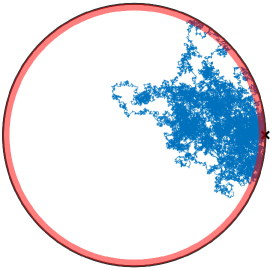
Figure 1: A simulated reflected Brownian motion with diffusion coefficient $D$ inside a disk of radius $R$, up to time $t=R^{2}/D$. Shadowed region is a thin layer near the boundary of width $a/R=0.05$. The residence time in this region, divided by $a$, is close to the boundary local time $\ell_{t}$, see Eq. (4). Black cross denotes the starting point of the trajectory.

In this paper, we provide a general description of the statistical properties of the boundary local time $\ell_{t}$. This description relies on the spectral theory of diffusion-reaction processes with heterogeneous surface reactivity developed in Grebenkov19 . In Sec. II, we derive a spectral representation for the probability density of the boundary local time $\ell_{t}$ in terms of the eigenvalues and eigenfunctions of the Dirichlet-to-Neumann operator. We also establish the asymptotic behavior of the probability density and of the moments of $\ell_{t}$. In Sec. III, our general results are illustrated for reflected Brownian motion inside and outside two archetypical confinements: a disk and a ball. Conclusions and perspectives of this work are discussed in Sec. IV.

II General theory

Our characterization of the boundary local time relies on two key results: the construction of partially reflected Brownian motion (Sec. II.1) and the spectral representation of the propagator via the Dirichlet-to-Neumann operator (Sec. II.2).

II.1 Partially reflected Brownian motion

In order to characterize the boundary local time $\ell_{t}$, we consider a more general partially reflected Brownian motion (PRBM) $\tilde{\bm{X}}_{t}$, whose heat kernel satisfies the diffusion equation

$$\partial_{t}G_{q}(\bm{x},t|\bm{x}_{0})=D\,\Delta_{\bm{x}}G_{q}(\bm{x},t|\bm{x}_{0})\qquad(\bm{x}\in\Omega)$$ (7)

for any $\bm{x}_{0}\in\bar{\Omega}$, subject to the initial condition $G_{q}(\bm{x},t=0|\bm{x}_{0})=\delta(\bm{x}-\bm{x}_{0})$ and the Robin (also known as Fourier, radiation or third) boundary condition

$$\partial_{n}G_{q}(\bm{x},t|\bm{x}_{0})+q\,G_{q}(\bm{x},t|\bm{x}_{0})=0\quad(\bm{x}\in\partial\Omega)$$ (8)

with a constant parameter

$$q=\kappa/D\geq 0$$

(see Papanicolaou90 ; Bass08 ; Zhou16 for mathematical details and references). When the domain $\Omega$ is unbounded, one also needs to impose a regularity condition at infinity: $G_{q}(\bm{x},t|\bm{x}_{0})\to 0$ as $|\bm{x}|\to\infty$ (similar condition has to be imposed for the related boundary value problems (12, 18, 19), see below).

The Robin boundary condition (8) appears in a large variety of physical, chemical and biological applications Collins49 ; Sano79 ; Sano81 ; Sapoval94 ; Benichou00 ; Sapoval02 ; Grebenkov05 ; Grebenkov06a ; Bressloff08 ; Singer08 ; Grebenkov10a ; Grebenkov10b ; Rojo12 ; Grebenkov15 , as well as the effective boundary condition after homogenization Zwanzig90 ; Berezhkovskii04 ; Berezhkovskii06 ; Muratov08 ; Dagdug16 ; Bernoff18b (see an overview in Grebenkov19b ). The subscript $q$ allows us to distinguish three types of boundary condition: Neumann ($q=0$), Robin ($0<q<\infty$), and Dirichlet ($q=\infty$). We note that the notation $G_{q}(\bm{x},t|\bm{x}_{0})$ is different from that of Refs. Grebenkov19 ; Grebenkov19b , in which Neumann and Dirichlet propagators were denoted as $G_{\kappa=0}$ and $G_{0}$, respectively.

The partially reflected Brownian motion $\tilde{\bm{X}}_{t}$ can be defined as reflected Brownian motion $\bm{X}_{t}$, which is stopped at the random time ${\mathcal{T}}$ of reaction. This stopping time is introduced by the following reasoning (see Grebenkov06 ; Grebenkov07a for details). At each arrival onto the boundary, the particle either reacts with the probability $p=1/(1+D/(\kappa a))$, or resumes bulk diffusion from a distance $a$ above the boundary, with the probability $1-p$ Filoche99 ; Grebenkov03 . Let $\hat{n}$ denote the random number of failed attempts (reflections) before successful reaction. As each reaction attempt is independent from the others, one has ${\mathbb{P}}\{\hat{n}=n\}=p(1-p)^{n}$ (with $n=0,1,2,\ldots$) and thus ${\mathbb{P}}\{\hat{n}\geq n\}=(1-p)^{n}\approx e^{-na\kappa/D}$ (for small $a$). Since $\hat{n}\approx\ell_{\mathcal{T}}/a$ due to Eq. (5), we set $\ell=na$ and thus get ${\mathbb{P}}\{\ell_{\mathcal{T}}\geq\ell\}=e^{-\ell\kappa/D}$ in the limit $a\to 0$; in other words, $\ell_{\mathcal{T}}$ obeys the exponential distribution with the mean $D/\kappa$. As the boundary local time is a nondecreasing process, the event $\{{\mathcal{T}}>t\}$ is identical to $\{\ell_{\mathcal{T}}>\ell_{t}\}$:

$${\mathbb{P}}_{\bm{x}_{0}}\{{\mathcal{T}}>t\}={\mathbb{P}}_{\bm{x}_{0}}\{\ell_{\mathcal{T}}>\ell_{t}\}\,.$$ (9)

As a consequence, the stopping time ${\mathcal{T}}$ can be defined as the first moment when the boundary local time $\ell_{t}$ exceeds a random threshold $\hat{\ell}$ ($=\ell_{\mathcal{T}}$):

$${\mathcal{T}}=\inf\{t>0~{}:~{}\ell_{t}>\hat{\ell}\},$$ (10)

where $\hat{\ell}$ is an independent exponential random variable with the mean $D/\kappa$. The independence follows from the fact that $\ell_{t}$ is determined by the dynamics of the particle, whereas $\hat{\ell}=\ell_{\mathcal{T}}$ is determined by the reactivity of the boundary.

The cumulative distribution function of the stopping time ${\mathcal{T}}$, ${\mathbb{P}}_{\bm{x}_{0}}\{{\mathcal{T}}\leq t\}$, is related to the survival probability of the particle,

$$S_{q}(t|\bm{x}_{0})={\mathbb{P}}_{\bm{x}_{0}}\{{\mathcal{T}}>t\}=1-{\mathbb{P}}_{\bm{x}_{0}}\{{\mathcal{T}}\leq t\},$$

which is obtained by integrating the propagator over the arrival point $\bm{x}$:

$$S_{q}(t|\bm{x}_{0})=\int\limits_{\Omega}d\bm{x}\,G_{q}(\bm{x},t|\bm{x}_{0}).$$ (11)

The survival probability also satisfies the diffusion equation with Robin boundary condition:

$$\partial_{t}S_{q}(t|\bm{x}_{0}) =D\Delta_{\bm{x}_{0}}S_{q}(t|\bm{x}_{0})\quad(\bm{x}_{0}\in\Omega),$$ (12a)

$$\partial_{n}S_{q}(t|\bm{x}_{0})+q\,S_{q}(t|\bm{x}_{0}) =0\quad(\bm{x}_{0}\in\partial\Omega),$$ (12b)

with the initial condition $S_{q}(t=0|\bm{x}_{0})=1$, that follows from Eqs. (7, 8) written in a backward form Redner ; Gardiner .

Since $\ell_{t}$ and $\hat{\ell}$ are independent by construction, the average over random realizations of $\hat{\ell}$ in Eq. (9) can be written as

$$S_{q}(t|\bm{x}_{0})=\int\limits_{0}^{\infty}d\ell\,\underbrace{e^{-q\ell}}_{={\mathbb{P}}\{\hat{\ell}>\ell\}}\,\rho(\ell,t|\bm{x}_{0})\,,$$ (13)

where $\rho(\ell,t|\bm{x}_{0})$ is the probability density function (PDF) of $\ell_{t}$ that we are looking for. Even though Eq. (13) fully determines $\rho(\ell,t|\bm{x}_{0})$ via the inverse Laplace transform with respect to $q$, the parameter $q$ is involved implicitly as the coefficient in Robin boundary condition (12b). As a consequence, even for simple domains like a disk or a ball, the above relation accesses the PDF of the boundary local time $\ell_{t}$ only numerically, and its practical implementation is time consuming. In the next section, we use a recently developed representation of the survival probability in the basis of the Dirichlet-to-Neumann operator Grebenkov19 in order to deduce a more explicit characterization of the boundary local time.

II.2 Spectral representation via Dirichlet-to-Neumann operator

The Laplace transform of Eq. (13) with respect to time $t$, denoted by tilde, reads

$$\tilde{S}_{q}(p|\bm{x}_{0})=\int\limits_{0}^{\infty}d\ell\,e^{-q\ell}\,\tilde{\rho}(\ell,p|\bm{x}_{0}).$$ (14)

Writing the survival probability in terms of the PDF of the stopping time ${\mathcal{T}}$, $H_{q}(t|\bm{x}_{0})$,

$${\mathbb{P}}_{\bm{x}_{0}}\{{\mathcal{T}}>t\}=1-\int\limits_{0}^{t}dt^{\prime}\,H_{q}(t^{\prime}|\bm{x}_{0}),$$ (15)

one gets

$$\frac{1-\tilde{H}_{q}(p|\bm{x}_{0})}{p}=\int\limits_{0}^{\infty}d\ell\,e^{-q\ell}\,\tilde{\rho}(\ell,p|\bm{x}_{0}),$$ (16)

where

$$\tilde{H}_{q}(p|\bm{x}_{0})={\mathbb{E}}_{\bm{x}_{0}}\{e^{-p{\mathcal{T}}}\}=\int\limits_{0}^{\infty}dt\,e^{-pt}\,H_{q}(t|\bm{x}_{0})$$ (17)

is the Laplace transform of $H_{q}(t|\bm{x}_{0})$, and ${\mathbb{E}}_{\bm{x}_{0}}$ denotes the expectation. Applying the Laplace transform to Eqs. (12, 15), one easily shows that $\tilde{H}_{q}(p|\bm{x}_{0})$ is the solution of the following boundary value problem:

$$(p-D\Delta_{\bm{x}_{0}})\tilde{H}_{q}(p|\bm{x}_{0}) =0\quad(\bm{x}_{0}\in\Omega),$$ (18a)

$$\biggl{(}\frac{1}{q}\partial_{n}\tilde{H}_{q}(p|\bm{x}_{0})+\tilde{H}_{q}(p|\bm{x}_{0})\biggr{)} =1\quad(\bm{x}_{0}\in\partial\Omega).$$ (18b)

It is therefore convenient to express it in terms of the spectral properties of the Dirichlet-to-Neumann operator ${\mathcal{M}}_{p}$ Grebenkov19 .

For a given function $f$ on the boundary $\partial\Omega$, the operator ${\mathcal{M}}_{p}$ associates another function on that boundary, ${\mathcal{M}}_{p}~{}:~{}f\mapsto g=(\partial_{n}u)_{|\partial\Omega}$, where $u$ is the solution of the modified Helmholtz equation subject to Dirichlet boundary condition:

$$(p-D\Delta)u(\bm{x}) = 0\quad(\bm{x}\in\Omega),$$ (19a)

$$u(\bm{x}) = f\quad(\bm{x}\in\partial\Omega).$$ (19b)

In physical terms, if $f$ prescribes a concentration of particles maintained on the boundary, then ${\mathcal{M}}_{p}f$ is proportional to the steady-state diffusive flux density of these particles into the bulk (with the bulk reaction rate $p$). In mathematical terms, for a given solution $u$ of the modified Helmholtz equation (19a), the operator ${\mathcal{M}}_{p}$ maps the Dirichlet boundary condition, $u|_{\partial\Omega}=f$, onto the equivalent Neumann boundary condition, $(\partial_{n}u)|_{\partial\Omega}=g={\mathcal{M}}_{p}f$. Note that there is a family of operators ${\mathcal{M}}_{p}$ parameterized by $p\geq 0$. For a smooth enough boundary $\partial\Omega$ (here we skip conventional mathematical restrictions and rigorous formulation of the involved functional spaces, see Egorov ; Jacob ; Taylor ; Marletta04 ; Arendt07 ; Arendt15 ; Hassell17 ; Girouard17 for details), ${\mathcal{M}}_{p}$ is well-defined pseudo-differential self-adjoint operator.

When the boundary is bounded, the spectrum of ${\mathcal{M}}_{p}$ is discrete, i.e., there are infinitely many eigenpairs $\{\mu_{n}^{(p)},\,v_{n}^{(p)}\}$, satisfying

$${\mathcal{M}}_{p}\,v_{n}^{(p)}=\mu_{n}^{(p)}\,v_{n}^{(p)}\quad(n=0,1,2,\ldots).$$ (20)

The eigenvalues $\mu_{n}^{(p)}$ are nonnegative and growing to infinity as $n\to\infty$, whereas the eigenfunctions $\{v_{n}^{(p)}\}$ form an orthonormal complete basis of the space $L_{2}(\partial\Omega)$ of square-integrable functions on $\partial\Omega$. In order to rely on this eigenbasis, we focus on bounded boundaries, whereas the confining domain $\Omega$ can be bounded or not. The limiting value of the smallest eigenvalue $\mu_{0}^{(p)}$ as $p\to 0$ distinguishes two types of diffusion: $\mu_{0}^{(0)}=0$ for recurrent motion (diffusion in a bounded domain in any dimension or diffusion in the exterior of a compact set for $d=2$) and $\mu_{0}^{(0)}>0$ for transient motion (diffusion in the exterior of a compact set for $d\geq 3$). Moreover, for diffusion in a bounded domain, the corresponding eigenfunction is constant: $v_{0}^{(0)}=|\partial\Omega|^{-1/2}$.

On one hand, the action of the Dirichlet-to-Neumann operator can be expressed by solving the boundary value problem (19) in a standard way with the help of the Laplace-transformed propagator $\tilde{G}_{\infty}(\bm{x},p|\bm{x}_{0})$ with Dirichlet boundary condition ($\kappa=\infty$):

$$[{\mathcal{M}}_{p}f](\bm{s}_{0})$$ (21)

$$=\biggl{(}\partial_{n_{0}}\int\limits_{\partial\Omega}d\bm{s}\,\bigl{(}-D\partial_{n}\tilde{G}_{\infty}(\bm{x},p|\bm{x}_{0})\bigr{)}_{\bm{x}=\bm{s}}\,f(\bm{s})\biggr{)}_{\bm{x}_{0}=\bm{s}_{0}}.$$

On the other hand, the inverse of the Dirichlet-to-Neumann operator for $p>0$ can be expressed in terms of the Laplace-transformed propagator $\tilde{G}_{0}(\bm{x},p|\bm{x}_{0})$ with Neumann boundary condition ($\kappa=0$) Grebenkov19 :

$$D\tilde{G}_{0}(\bm{s},p|\bm{s}_{0})={\mathcal{M}}_{p}^{-1}\delta(\bm{s}-\bm{s}_{0})\quad(\bm{s},\bm{s}_{0}\in\partial\Omega)$$ (22)

(note that ${\mathcal{M}}_{0}$ is not invertible for bounded domains). We hasten to outline a slight abuse of notation here and throughout the paper: on the left-hand side of Eq. (22), boundary points $\bm{s}$ and $\bm{s}_{0}$ are understood as points in ${\mathbb{R}}^{d}$ restricted to $\partial\Omega$; on the right-hand side, boundary points $\bm{s}$ and $\bm{s}_{0}$ are understood as points on a $(d-1)$-dimensional manifold $\partial\Omega$, on which the Dirichlet-to-Neumann operator acts. In particular, the Laplace-transformed propagator has units of second $\cdot$ meter^-d, whereas the Dirac distribution has units of meter^1-d.

Now we come back to the problem of finding the solution of Eqs. (18). As shown in Grebenkov19 , $\tilde{H}_{q}(p|\bm{x}_{0})$ admits the following spectral representation:

$$\tilde{H}_{q}(p|\bm{x}_{0})=\sum\limits_{n=0}^{\infty}\frac{V_{n}^{(p)}(\bm{x}_{0})\int\nolimits_{\partial\Omega}d\bm{s}\,[v_{n}^{(p)}(\bm{s})]^{*}}{1+\mu_{n}^{(p)}/q}\,,$$ (23)

where asterisk denotes complex conjugate, and

$$V_{n}^{(p)}(\bm{x}_{0})=\int\limits_{\partial\Omega}d\bm{s}\,\tilde{j}_{\infty}(\bm{s},p|\bm{x}_{0})\,v_{n}^{(p)}(\bm{s}),$$ (24)

with $\tilde{j}_{\infty}(\bm{s},p|\bm{x}_{0})=-D\bigl{(}\partial_{n}\tilde{G}_{\infty}(\bm{x},p|\bm{x}_{0})\bigr{)}_{\bm{x}=\bm{s}}$ being the Laplace transform of the probability flux density onto a perfectly absorbing boundary (with Dirichlet boundary condition, $\kappa=\infty$).

If the starting point $\bm{x}_{0}$ lies in the bulk $\Omega$, any trajectory of the PRBM $\tilde{\bm{X}}_{t}$ can be split into two successive paths: from $\bm{x}_{0}$ to a first hitting point $\bm{s}_{0}$ on the boundary, and from $\bm{s}_{0}$ to a boundary point $\bm{s}$, at which the process is stopped. The stopping time ${\mathcal{T}}$ is thus the sum of two random durations of these paths. Along the first path, the boundary local time $\ell_{t}$ remains zero and thus is not informative. As first-passage times to a boundary were thoroughly investigated in the past, it is convenient to exclude this contribution from our analysis and to focus on the second, much more complicated and less studied random variable. For this reason, we assume in the following that the starting point $\bm{x}_{0}$ lies on the boundary, i.e., $\bm{x}_{0}=\bm{s}_{0}\in\partial\Omega$. In this case, $\tilde{j}_{\infty}(\bm{s},p|\bm{s}_{0})=\delta(\bm{s}-\bm{s}_{0})$ and thus $V_{n}^{(p)}(\bm{s}_{0})=v_{n}^{(p)}(\bm{s}_{0})$ so that Eq. (23) is reduced to

$$\tilde{H}_{q}(p|\bm{s}_{0})=\sum\limits_{n=0}^{\infty}\frac{\hat{v}_{n}^{(p)}(\bm{s}_{0})}{1+\mu_{n}^{(p)}/q}\,.$$ (25)

where

$$\hat{v}_{n}^{(p)}(\bm{s}_{0})=v_{n}^{(p)}(\bm{s}_{0})\,\int\limits_{\partial\Omega}d\bm{s}\,[v_{n}^{(p)}(\bm{s})]^{*}$$ (26)

are just the rescaled eigenfunctions $v_{n}^{(p)}(\bm{s}_{0})$. Once $\tilde{H}_{q}(p|\bm{s}_{0})$ (or related quantity) is known for a starting point $\bm{s}_{0}$ on the boundary, one can easily extend it to any starting point $\bm{x}_{0}$ in the bulk using the relation:

$$\tilde{H}_{q}(p|\bm{x}_{0})=\int\limits_{\partial\Omega}d\bm{s}_{0}\,\tilde{j}_{\infty}(\bm{s}_{0},p|\bm{x}_{0})\,\tilde{H}_{q}(p|\bm{s}_{0}),$$ (27)

which follows from Eqs. (23, 24, 25). In particular, this relation applied to Eq. (14) gives

$$\underbrace{\int\limits_{0}^{\infty}d\ell\,e^{-q\ell}\,\tilde{\rho}(\ell,p|\bm{x}_{0})}_{=\tilde{S}_{q}(p|\bm{x}_{0})}=\tilde{S}_{\infty}(p|\bm{x}_{0})$$

$$+\int\limits_{\partial\Omega}d\bm{s}_{0}\,\tilde{j}_{\infty}(\bm{s}_{0},p|\bm{x}_{0})\underbrace{\int\limits_{0}^{\infty}d\ell\,e^{-q\ell}\,\tilde{\rho}(\ell,p|\bm{s}_{0})}_{=\tilde{S}_{q}(p|\bm{s}_{0})},$$

from which the inverse Laplace transform with respect to $q$ yields

$$\tilde{\rho}(\ell,p|\bm{x}_{0})=\tilde{S}_{\infty}(p|\bm{x}_{0})\,\delta(\ell)+\int\limits_{\partial\Omega}d\bm{s}_{0}\,\tilde{j}_{\infty}(\bm{s}_{0},p|\bm{x}_{0})\,\tilde{\rho}(\ell,p|\bm{s}_{0}),$$ (28)

whereas the inverse Laplace transform with respect to $p$ leads to

$$\rho(\ell,t|\bm{x}_{0}) =S_{\infty}(t|\bm{x}_{0})\,\delta(\ell)$$ (29)

$$+\int\limits_{\partial\Omega}d\bm{s}_{0}\int\limits_{0}^{t}dt^{\prime}\,j_{\infty}(\bm{s}_{0},t^{\prime}|\bm{x}_{0})\,\rho(\ell,t-t^{\prime}|\bm{s}_{0}).$$

This relation has a simple probabilistic interpretation. When the particle starts from a bulk point $\bm{x}_{0}\in\Omega$, the boundary local time remains zero until the first arrival onto the boundary. As a consequence, the probability distribution of $\ell_{t}$ has an atom at $\ell=0$, i.e., $\ell_{t}$ is zero with a finite probability, which is equal to the survival probability $S_{\infty}(t|\bm{x}_{0})$ (the first term). In turn, the positive values of $\ell_{t}$ are given by the convolution of the probability density of arriving at $\bm{s}_{0}$ at time $t^{\prime}$ with the probability density of getting $\ell$ within the remaining time $t-t^{\prime}$ from the starting point $\bm{s}_{0}$ (the second term). As Eq. (29) expresses the probability density $\rho(\ell,t|\bm{x}_{0})$ for any bulk point $\bm{x}_{0}$ in terms of $\rho(\ell,t|\bm{s}_{0})$ for a boundary point $\bm{s}_{0}$, we focus on the latter quantity in the reminder of the paper.

The completeness of eigenfunctions $v_{n}^{(p)}$ implies the identity

$$\sum\limits_{n=0}^{\infty}\hat{v}_{n}^{(p)}(\bm{s}_{0})=1.$$ (30)

Using this representation of $1$, one can rewrite Eq. (16) as

$$\frac{1}{p}\sum\limits_{n=0}^{\infty}\hat{v}_{n}^{(p)}(\bm{s}_{0})\frac{\mu_{n}^{(p)}}{\mu_{n}^{(p)}+q}=\int\limits_{0}^{\infty}d\ell\,e^{-q\ell}\,\tilde{\rho}(\ell,p|\bm{s}_{0})\,,$$ (31)

from which

$$\tilde{\rho}(\ell,p|\bm{s}_{0})=\frac{1}{p}\sum\limits_{n=0}^{\infty}\hat{v}_{n}^{(p)}(\bm{s}_{0})\,\mu_{n}^{(p)}\,e^{-\mu_{n}^{(p)}\ell}\,.$$ (32)

The inverse Laplace transform with respect to $p$ yields the PDF $\rho(\ell,t|\bm{s}_{0})$ of the boundary local time $\ell_{t}$:

$$\rho(\ell,t|\bm{s}_{0})={\mathcal{L}}^{-1}_{t}\biggl{\{}\frac{1}{p}\sum\limits_{n=0}^{\infty}\hat{v}_{n}^{(p)}(\bm{s}_{0})\,\mu_{n}^{(p)}\,e^{-\mu_{n}^{(p)}\ell}\biggr{\}}\,.$$ (33)

Since

$$\rho(\ell,t|\bm{s}_{0})=-\frac{\partial{\mathbb{P}}_{\bm{s}_{0}}\{\ell_{t}>\ell\}}{\partial\ell}\,,$$ (34)

the integral of Eq. (32) from $\ell$ to infinity gives

$$\int\limits_{0}^{\infty}dt\,e^{-pt}\,{\mathbb{P}}_{\bm{s}_{0}}\{\ell_{t}>\ell\}=\frac{1}{p}\sum\limits_{n=0}^{\infty}\hat{v}_{n}^{(p)}(\bm{s}_{0})\,e^{-\mu_{n}^{(p)}\ell}\,,$$ (35)

and thus

$${\mathbb{P}}_{\bm{s}_{0}}\{\ell_{t}>\ell\}={\mathcal{L}}^{-1}_{t}\left\{\frac{1}{p}\sum\limits_{n=0}^{\infty}\hat{v}_{n}^{(p)}(\bm{s}_{0})\,e^{-\mu_{n}^{(p)}\ell}\right\}\,.$$ (36)

Either of Eqs. (32, 35) fully determines the distribution of the boundary local time $\ell_{t}$. These are the main results of the paper. While we treated the boundary as reactive to define the stopping time ${\mathcal{T}}$ and to perform the above derivation, the final results (32, 35) do not depend on the reactivity $\kappa$. Indeed, these relations determine the boundary local time and thus characterize the dynamics near reflecting boundary, which is disentangled from eventual surface reactions. Note that Eq. (30) implies ${\mathbb{P}}_{\bm{s}_{0}}\{\ell_{t}>0\}=1$ that is equivalent to the normalization of the probability density $\rho(\ell,t|\bm{s}_{0})$.

The relation (32) also determines the positive moments of the boundary local time in the Laplace domain:

$$\int\limits_{0}^{\infty}dt\,e^{-pt}\,{\mathbb{E}}_{\bm{s}_{0}}\{\ell_{t}^{k}\}=\frac{k!}{p}\sum\limits_{n=0}^{\infty}\frac{\hat{v}_{n}^{(p)}(\bm{s}_{0})}{[\mu_{n}^{(p)}]^{k}}\,.$$ (37)

II.3 Short-time behavior

For $k=1$, the sum in the right-hand side of Eq. (37) can be seen as the spectral representation of the inverse of the Dirichlet-to-Neumann operator, ${\mathcal{M}}_{p}^{-1}$, which is equal to $D\tilde{G}_{0}(\bm{s},p|\bm{s}_{0})$ according to Eq. (22). As a consequence, the Laplace transform can be inverted to get

$${\mathbb{E}}_{\bm{s}_{0}}\{\ell_{t}\}=\int\limits_{0}^{t}dt^{\prime}\,\int\limits_{\partial\Omega}d\bm{s}\,DG_{0}(\bm{s},t^{\prime}|\bm{s}_{0})\,.$$ (38)

This representation also follows directly from the general formula for the residence time and its limiting form in Eq. (4). In the short-time limit, the propagator can be locally approximated by that near a reflecting hyperplane,

$$G_{0}(\bm{s},t|\bm{s}_{0})\simeq\frac{\exp\bigl{(}-|\bm{s}-\bm{s}_{0}|^{2}/(4Dt)\bigr{)}}{(4\pi Dt)^{(d-1)/2}}\,\frac{1}{\sqrt{\pi Dt}}\,,$$ (39)

where the second factor accounts for the orthogonal direction. Integrating this function over $\bm{s}\in{\mathbb{R}}^{d-1}$, one gets from Eq. (38):

$${\mathbb{E}}_{\bm{s}_{0}}\{\ell_{t}\}\simeq 2\sqrt{Dt}/\sqrt{\pi}\qquad(t\to 0).$$ (40)

Here, the short-time behavior does not depend on the starting point $\bm{s}_{0}$ because the boundary locally looks flat as $t\to 0$. This asymptotic behavior agrees with the upper bound provided in Hsu85 . Qualitatively, this universal asymptotic behavior can be rationalized as following. At short times, the particle moves away from the boundary by a distance of the order of $\sqrt{Dt}$, i.e., the typical available volume is $(\sqrt{Dt})^{d}$ (here, we omit eventual numerical prefactors), in which the residence time is close to $t$. The mean residence time in a thin boundary layer of width $a$ and of lateral radius $\sqrt{Dt}$, whose volume is of the order $a(\sqrt{Dt})^{d-1}$, is the total residence time (close to $t$), multiplied by the ratio of these volumes: $t\,a(\sqrt{Dt})^{d-1}/(\sqrt{Dt})^{d}$. According to Eq. (4), the mean boundary local time is then $\sqrt{Dt}$, up to the numerical constant (given in Eq. (40)).

II.4 Long-time behavior

To study the long-time behavior, we distinguish three cases.

Diffusion in a bounded domain

Diffusion in a bounded domain is recurrent in any space ${\mathbb{R}}^{d}$ so that $\mu_{0}^{(p)}\to 0$ as $p\to 0$. More precisely, one has (see Appendix A)

$$\mu_{0}^{(p)}\simeq\frac{p}{D}\,\frac{|\Omega|}{|\partial\Omega|}\qquad(p\to 0)$$ (41)

(here $|A|$ is the Lebesgue measure of $A$), while $v_{0}^{(p)}\to v_{0}^{(0)}=|\partial\Omega|^{-1/2}$ so that the orthogonality of eigenfunctions $\{v_{n}^{(0)}\}$ simplifies Eq. (37) and yields

$${\mathbb{E}}_{\bm{s}_{0}}\{\ell_{t}^{k}\}\simeq(Dt|\partial\Omega|/|\Omega|)^{k}\qquad(t\to\infty).$$ (42)

As expected, these moments grow up to infinity as $t\to\infty$, and the long-time asymptotic behavior does not depend on the starting point $\bm{s}_{0}$. In particular, the linear growth of the mean boundary local time with $t$ has a simple explanation: at long times, the particle is uniformly distributed in the bounded domain and thus spends in a thin boundary layer $\partial\Omega_{a}$ a fraction of time, which is proportional to the volume of $\partial\Omega_{a}$ divided by the volume of the domain $\Omega$. In other words, the mean residence time in $\partial\Omega_{a}$ is approximately $t|\partial\Omega_{a}|/|\Omega|\approx ta|\partial\Omega|/|\Omega|$, from which Eq. (4) yields ${\mathbb{E}}_{\bm{s}_{0}}\{\ell_{t}\}\simeq Dt|\partial\Omega|/|\Omega|$, in agreement with Eq. (42).

In Grebenkov07a , a much stronger property was established: all the cumulant moments of $\ell_{t}$ grow linearly with time $t$. As a consequence, the distribution of the boundary local time is asymptotically close to a Gaussian distribution in the limit $t\to\infty$:

$$\rho(\ell,t|\bm{s}_{0})\simeq\frac{\exp\bigl{(}-\frac{(\ell-Dt|\partial\Omega|/|\Omega|)^{2}}{2b_{2,1}t}\bigr{)}}{\sqrt{2\pi b_{2,1}t}}\quad(t\to\infty),$$ (43)

where the constant $b_{2,1}$ was formally computed in Grebenkov07a . In Appendix B, we express this constant in terms of the second derivative of the smallest eigenvalue $\mu_{0}^{(p)}$ with respect to $p$ (evaluated at $p=0$):

$$b_{2,1}=-\biggl{(}\frac{D|\partial\Omega|}{|\Omega|}\biggr{)}^{3}\lim\limits_{p\to 0}\frac{d^{2}\mu_{0}^{(p)}}{dp^{2}}\,.$$ (44)

Diffusion in the exterior of a compact planar set

When $\Omega$ is the exterior of a compact planar set, diffusion is still recurrent, and $\mu_{0}^{(p)}\to 0$ as $p\to 0$. However, the approach to zero is much slower than in Eq. (37). In this setting, the mean boundary local time also grows up to infinity but much slower (see Sec. III.3 for an example in the exterior of a disk).

Diffusion in the exterior of a compact set in higher dimensions

When $\Omega$ is the exterior of a compact set in ${\mathbb{R}}^{d}$ with $d\geq 3$, one has $\mu_{0}^{(p)}\to\mu_{0}^{(0)}>0$ as $p\to 0$, diffusion is transient, i.e., the particle will ultimately escape to infinity and never return. As a consequence, Eq. (35) implies

$${\mathbb{P}}_{\bm{s}_{0}}\{\ell_{t}>\ell\}\to{\mathbb{P}}_{\bm{s}_{0}}\{\ell_{\infty}>\ell\}\qquad(t\to\infty),$$ (45)

with

$${\mathbb{P}}_{\bm{s}_{0}}\{\ell_{\infty}>\ell\}=\sum\limits_{n=0}^{\infty}\hat{v}_{n}^{(0)}(\bm{s}_{0})\,e^{-\mu_{n}^{(0)}\ell}\,.$$ (46)

In other words, the boundary local time reaches its steady-state limit $\ell_{\infty}$ determined by the above distribution and the following moments:

$${\mathbb{E}}_{\bm{s}_{0}}\{\ell_{\infty}^{k}\}=k!\sum\limits_{n=0}^{\infty}\frac{\hat{v}_{n}^{(0)}(\bm{s}_{0})}{[\mu_{n}^{(0)}]^{k}}\,.$$ (47)

We emphasize that $v_{n}^{(0)}(\bm{s})$ is not in general constant for exterior diffusion so that all eigenmodes can contribute.

II.5 A probabilistic interpretation

Introducing an independent exponentially distributed random stopping time $\tau$, defined by the rate $p$ as ${\mathbb{P}}\{\tau>t\}=e^{-pt}$, one can multiply the left-hand side of Eq. (35) by $p$ and interpret it as the average over the exponential stopping time $\tau$ (with the probability density $p\,e^{-pt}$)

$${\mathbb{P}}_{\bm{s}_{0}}\{\ell_{\tau}>\ell\}=\int\limits_{0}^{\infty}dt\,p\,e^{-pt}\,{\mathbb{P}}_{\bm{s}_{0}}\{\ell_{t}>\ell\}.$$ (48)

In other words, we get explicitly the probability law for the boundary local time $\ell_{\tau}$ stopped at an exponentially distributed time $\tau$:

$${\mathbb{P}}_{\bm{s}_{0}}\{\ell_{\tau}>\ell\}=\sum\limits_{n=0}^{\infty}\hat{v}_{n}^{(p)}(\bm{s}_{0})\,e^{-\mu_{n}^{(p)}\ell}\,.$$ (49)

Similarly, Eq. (37) yields the moments of the boundary local time stopped at $\tau$:

$${\mathbb{E}}_{\bm{s}_{0}}\{\ell_{\tau}^{k}\}=k!\sum\limits_{n=0}^{\infty}\frac{\hat{v}_{n}^{(p)}(\bm{s}_{0})}{[\mu_{n}^{(p)}]^{k}}\,.$$ (50)

The probabilistic interpretation of $\ell_{\tau}$ is rather straightforward in terms of “mortal walkers” Yuste13 ; Meerson15 ; Grebenkov17d . In fact, one can consider a particle that diffuses in a reactive bulk and can spontaneously disappear with the rate $p$. In this setting, $\tau$ is the random lifetime of such a mortal walker.

III Examples

In this section, we illustrate the properties of the boundary local time with five examples, for which the eigenbasis of the Dirichlet-to-Neumann operator is known explicitly. The probability density function $\rho(\ell,t|\bm{s}_{0})$ is then obtained by the numerical inversion of the Laplace transform in Eq. (33) using the Talbot algorithm. The accuracy of this numerical computation was validated by Monte Carlo simulations presented in Appendix C.

III.1 Half-space

The simplest setting for the analysis of the boundary local time $\ell_{t}$ is the half-space ${\mathbb{R}}^{d}_{+}$. Formally, one would need to consider the Dirichlet-to-Neumann operator on a hyperplane which is the boundary of this domain, and thus to deal with continuous spectrum. However, the translational invariance of the half-space implies that the lateral motion along the hyperplane is independent of the transverse motion, which thus fully determines $\ell_{t}$. In other words, the boundary local time on a hyperplane is identical to that on the endpoint of the positive half-line ${\mathbb{R}}_{+}=(0,+\infty)$ with reflections at $0$. The latter is twice the local time of Brownian motion at zero that was thoroughly investigated starting from the seminal works by P. Lévy Levy (see also Takacs95 ).

For illustrative purposes, we rederive its distribution from our general approach. The derivation is particularly simple because the boundary of the half-line is just a single point so that the Dirichlet-to-Neumann operator acts on a one-dimensional space of functions. In fact, a general solution of the modified Helmholtz equation (19a) is $u(x)=f\,\exp(-x\sqrt{p/D})$ with a constant $f$ set by the boundary condition (19b), while its normal derivative at zero is $f\sqrt{p/D}$. The action of ${\mathcal{M}}_{p}$ is thus the multiplication of a function at the boundary, namely, a constant $f$, by $\sqrt{p/D}$. There exists a single eigenvalue of ${\mathcal{M}}_{p}$, $\mu_{0}^{(p)}=\sqrt{p/D}$, with the corresponding eigenfunction $v_{0}^{(p)}=1$. According to Eq. (33), the probability density of the boundary local time is then

$$\rho(\ell,t)={\mathcal{L}}^{-1}_{t}\left\{\frac{\sqrt{p/D}}{p}\,e^{-\ell\sqrt{p/D}}\right\}=\frac{\exp\bigl{(}-\frac{\ell^{2}}{4Dt}\bigr{)}}{\sqrt{\pi Dt}}\,.$$ (51)

A similar computation can be undertaken for an interval.

III.2 Interior of a disk

We then study the local time on the boundary $\partial\Omega$ of a disk of radius $R$, $\Omega=\{\bm{x}\in{\mathbb{R}}^{2}~{}:~{}|\bm{x}|<R\}$. Even though the eigenmodes of the Dirichlet-to-Neumann operator ${\mathcal{M}}_{p}$ are well known for this domain, we rederive them to illustrate the method. For this purpose, one needs to solve the Dirichlet boundary value problem (19). Due to the rotational symmetry of the domain $\Omega$, one can search a general solution of the modified Helmholtz equation (19a) in polar coordinates $(r,\theta)$ in the form

$$u(r,\theta)=\sum\limits_{n=-\infty}^{\infty}c_{n}\,I_{n}(r\sqrt{p/D})\,e^{in\theta},$$ (52)

where $I_{n}(z)$ are the modified Bessel functions of the first kind, and the coefficients $c_{n}$ are fixed by the Dirichlet condition (19b) with a given function $f$:

$$c_{n}=\frac{1}{I_{n}(R\sqrt{p/D})}\int\limits_{0}^{2\pi}\frac{d\theta}{2\pi}f(\theta)\,e^{-in\theta}.$$ (53)

As the normal derivative acts only on the radial coordinate, $\partial_{n}=\partial_{r}$, the action of ${\mathcal{M}}_{p}$ onto $f$ reads

$${\mathcal{M}}_{p}f =\bigl{(}\partial_{n}u(r,\theta)\bigr{)}_{|\partial\Omega}$$

$$=\sum\limits_{n=-\infty}^{\infty}\frac{\sqrt{p/D}\,I^{\prime}_{n}(R\sqrt{p/D})}{I_{n}(R\sqrt{p/D})}\,e^{in\theta}\int\limits_{0}^{2\pi}\frac{d\theta}{2\pi}f(\theta)\,e^{-in\theta},$$

where prime denotes the derivative with respect to the argument. Setting $f(\theta)=e^{in\theta}$, one has

$${\mathcal{M}}_{p}e^{in\theta}=\frac{\sqrt{p/D}\,I^{\prime}_{n}(R\sqrt{p/D})}{I_{n}(R\sqrt{p/D})}\,e^{in\theta}\,,$$ (54)

i.e., $e^{in\theta}$ is an eigenfunction of ${\mathcal{M}}_{p}$ for any $n\in{\mathbb{Z}}$, whereas

$$\mu_{n}^{(p)}=\sqrt{p/D}\,\frac{I^{\prime}_{n}(R\sqrt{p/D})}{I_{n}(R\sqrt{p/D})}$$ (55)

is the corresponding eigenvalue. We emphasize that the form of the eigenfunctions is a direct consequence of the rotational symmetry of the domain. For coherence with the general description in Sec. II, we substitute the angular coordinate $\theta$ by the curvilinear coordinate $s/R$, with $s$ ranging from $0$ to $2\pi R$ along the circular boundary $\partial\Omega$,

$$v_{n}^{(p)}(s)=\frac{e^{ins/R}}{\sqrt{2\pi R}}\qquad(n\in{\mathbb{Z}}),$$ (56)

in which the $L_{2}(\partial\Omega)$-normalization is also incorporated. In this particular example, the eigenfunctions do not depend on $p$, whereas the eigenvalues are twice degenerate, except for $n=0$. Here, the index $n$ runs over all integer numbers for convenience of enumeration.

The orthogonality of the harmonics $\{e^{ins/R}\}$ to a constant implies that only the term with $n=0$ survives in Eqs. (32, 35), yielding

$${\mathbb{P}}_{\bm{s}_{0}}\{\ell_{t}>\ell\}={\mathcal{L}}^{-1}_{t}\left\{\frac{1}{p}\exp\left(-\ell\sqrt{p/D}\frac{I_{1}(R\sqrt{p/D})}{I_{0}(R\sqrt{p/D})}\right)\right\},$$ (57)

from which $\rho(\ell,t)$ is found via Eq. (34). As expected, this result does not depend on the starting point $\bm{s}_{0}$ on the circle. The mean boundary local time from Eq. (37) reads

$${\mathbb{E}}\{\ell_{t}\}={\mathcal{L}}^{-1}_{t}\left\{\frac{1}{p}\,\frac{I_{0}(R\sqrt{p/D})}{\sqrt{p/D}\,I_{1}(R\sqrt{p/D})}\right\}\,.$$ (58)

From this expression, one easily retrieves the short-time and long-time asymptotic behaviors: ${\mathbb{E}}\{\ell_{t}\}\simeq 2\sqrt{Dt}/\sqrt{\pi}$ as $t\to 0$ and ${\mathbb{E}}\{\ell_{t}\}\simeq 2Dt/R$ as $t\to\infty$, in agreement with Eqs. (40, 42). We emphasize that Eqs. (57, 58) also characterize the boundary local time of reflected Brownian motion inside a cylinder of radius $R$ (given that displacements along the cylinder axis do not affect the boundary local time). In particular, $\ell_{t}$ determines the residence time in a thin cylindrical layer and the number of returns to this layer.

Figure 2a shows the probability density function $\rho(\ell,t)$ for different times $t$. One can notice that $\rho(\ell,t)$ exhibits a maximum, which is progressively shifted toward larger $\ell$ with time. At short times (blue curves), the PDF is flat at small $\ell$, and then rapidly drops at large $\ell$. As time $t$ increases, the shape of the PDF transforms and becomes more localized near the mean boundary local time. At long times (red curves), the PDF is getting close to a Gaussian distribution (43), with the linearly growing mean and variance, as discussed in Sec. II.4.

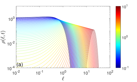
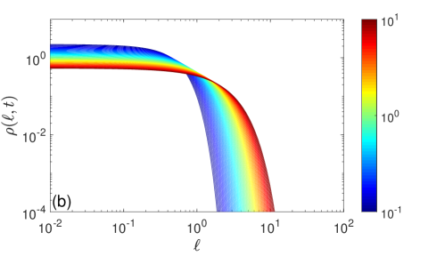
Figure 2: Probability density function $\rho(\ell,t)$ of the boundary local time $\ell_{t}$ for a disk of radius $R=1$, with $D=1$ and $t$ taking 64 logarithmically spaced values from $10^{-1}$ (dark blue) to $10^{1}$ (dark red). (a) diffusion inside the disk; (b) diffusion outside the disk.

III.3 Exterior of a disk

For the exterior of a disk of radius $R$, $\Omega=\{\bm{x}\in{\mathbb{R}}^{2}~{}:~{}|\bm{x}|>R\}$, the eigenfunctions of the Dirichlet-to-Neumann operator remain unchanged (as a consequence of the preserved rotational symmetry), whereas the eigenvalues are

$$\mu_{n}^{(p)}=-\sqrt{p/D}\frac{K^{\prime}_{n}(R\sqrt{p/D})}{K_{n}(R\sqrt{p/D})}\qquad(n\in{\mathbb{Z}})\,,$$ (59)

where $K_{n}(z)$ are the modified Bessel functions of the second kind. Indeed, one can repeat the derivation from Sec. III.2 by replacing $I_{n}(r\sqrt{p/D})$ in Eq. (52) by $K_{n}(r\sqrt{p/D})$, which vanish as $r\to\infty$, and using $\partial_{n}=-\partial_{r}$, which results in the negative sign in Eq. (59).

As previously, the orthogonality of eigenfunctions reduces Eq. (35) to

$${\mathbb{P}}_{\bm{s}_{0}}\{\ell_{t}>\ell\}={\mathcal{L}}^{-1}_{t}\biggl{\{}\frac{1}{p}\exp\biggl{(}-\ell\sqrt{p/D}\frac{K_{1}(R\sqrt{p/D})}{K_{0}(R\sqrt{p/D})}\biggr{)}\biggr{\}},$$ (60)

whereas the probability density $\rho(\ell,t)$ follows from Eq. (34). The mean boundary local time is

$${\mathbb{E}}\{\ell_{t}\}={\mathcal{L}}^{-1}_{t}\left\{\frac{1}{p}\,\frac{K_{0}(R\sqrt{p/D})}{\sqrt{p/D}\,K_{1}(R\sqrt{p/D})}\right\}\,.$$ (61)

We note that Eqs. (60, 61) also characterize the boundary local time of reflected Brownian motion outside a cylinder of radius $R$. For instance, $\ell_{t}$ describes the number of bulk relocations on a cylindrical strand, which is relevant, e.g., in a field cycling NMR dispersion technique Levitz08 .

The short-time behavior is the same as for the interior problem: ${\mathbb{E}}\{\ell_{t}\}\simeq 2\sqrt{Dt}/\sqrt{\pi}$, in agreement with Eq. (40). In turn, the long-time behavior is different, as can be seen by looking at the limit $p\to 0$. The asymptotic properties of the modified Bessel functions imply that the smallest eigenvalue $\mu_{0}^{(p)}$ approaches $0$ logarithmically slowly:

$$\mu_{0}^{(p)}\simeq\frac{1}{R(-\ln(R\sqrt{p/D}/2)-\gamma)}\qquad(p\to 0),$$ (62)

where $\gamma\approx 0.5772\ldots$ is the Euler constant. As a consequence,

$${\mathbb{E}}\{\ell_{t}\}\simeq R\bigl{(}\ln(\sqrt{4Dt}/R)-\gamma/2\bigr{)}+o(1)\quad(t\to\infty),$$ (63)

i.e., the boundary local time continues to grow (in agreement with the recurrent character of two-dimensional Brownian motion) but the growth is logarithmically slow.

It is also instructive to determine the long-time asymptotic behavior of the variance of $\ell_{t}$. Substituting Eq. (62) into Eq. (37) with $k=2$, one gets as $t\to\infty$:

$${\mathbb{E}}\{\ell_{t}^{2}\}\simeq 2R^{2}{\mathcal{L}}^{-1}_{t}\left\{\frac{(-\ln(R\sqrt{p/D}/2)-\gamma)^{2}}{p}\right\}$$

$$\simeq R^{2}\left\{2\biggl{(}\ln(\sqrt{4Dt}/R)-\gamma/2\biggr{)}^{2}-\frac{\pi^{2}}{12}+o(1)\right\},$$

so that

$${\rm var}\{\ell_{t}\}\simeq R^{2}\left\{\biggl{(}\ln(\sqrt{4Dt}/R)-\gamma/2\biggr{)}^{2}-\frac{\pi^{2}}{12}+o(1)\right\}.$$ (64)

The relative width of the distribution, $\sqrt{{\rm var}\{\ell_{t}\}}/{\mathbb{E}}\{\ell_{t}\}$, slowly approaches $1$ in this limit.

Figure 2b illustrates the behavior of $\rho(\ell,t)$, which is drastically different from the case of diffusion inside the disk (Fig. 2a). The PDF does not have a maximum. At any time $t$, $\rho(\ell,t)$ exhibits a flat behavior at small $\ell$ and then drops at large $\ell$. Moreover, the curves are getting very close to each other at long times. Even though this observation may suggest an approach to a steady-state limit, this is not the case, given that the mean boundary local time slowly grows, see Eq. (63).

In a similar way, one can derive the exact distribution of the boundary local time for an annulus between two concentric circles. Moreover, one can look for the local time on each circle or impose an absorbing boundary condition on one of the circles. In all these cases, the eigenfunctions of the Dirichlet-to-Neumann operator remain unchanged, while the eigenvalues can be written explicitly in terms of modified Bessel functions.

III.4 Interior of a ball

For the ball of radius $R$, $\Omega=\{\bm{x}\in{\mathbb{R}}^{3}~{}:~{}|\bm{x}|<R\}$, the eigenfunctions of the Dirichlet-to-Neumann operator are the (normalized) spherical harmonics, $Y_{mn}(\theta,\phi)/R$ (with $n=0,1,2,\ldots$ and $m=-n,\ldots,n$), whereas the eigenvalues are

$$\mu_{n}^{(p)}=\sqrt{p/D}\,\frac{i^{\prime}_{n}(R\sqrt{p/D})}{i_{n}(R\sqrt{p/D})}\quad(n=0,1,2,\ldots),$$ (65)

where $i_{n}(z)$ are the modified spherical Bessel functions of the first kind. The orthogonality of spherical harmonics to a constant function reduces Eq. (35) to

$${\mathbb{P}}_{\bm{s}_{0}}\{\ell_{t}>\ell\}$$ (66)

$$={\mathcal{L}}^{-1}_{t}\left\{\frac{1}{p}\exp\left(-\ell\biggl{(}\sqrt{p/D}\,\mathrm{ctanh}(R\sqrt{p/D})-1/R\biggr{)}\right)\right\},$$

where we used the explicit form $i_{0}(z)=\sinh(z)/z$. The probability density $\rho(\ell,t)$ follows from Eq. (34).

Figure 3a illustrates the behavior of $\rho(\ell,t)$, which is very similar to the case of diffusion inside a disk (Fig. 2a).

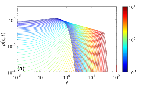
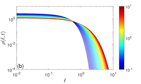
Figure 3: Probability density functions $\rho(\ell,t)$ of the boundary local time $\ell_{t}$ for a ball of radius $R=1$, with $D=1$ and $t$ taking 64 logarithmically spaced values from $10^{-1}$ (dark blue) to $10^{1}$ (dark red). (a) diffusion inside the ball, (b) diffusion outside the ball.

III.5 Exterior of a ball

For the exterior of a ball of radius $R$, $\Omega=\{\bm{x}\in{\mathbb{R}}^{3}~{}:~{}|\bm{x}|>R\}$, the eigenfunctions of the Dirichlet-to-Neumann operator remain unchanged, whereas the eigenvalues are

$$\mu_{n}^{(p)}=-\sqrt{p/D}\,\frac{k^{\prime}_{n}(R\sqrt{p/D})}{k_{n}(R\sqrt{p/D})}\quad(n=0,1,2,\ldots),$$ (67)

where $k_{n}(z)$ are the modified spherical Bessel functions of the second kind. Interestingly, the eigenvalues are just polynomials of $\sqrt{p/D}$, e.g., $\mu_{0}^{(p)}=(1+R\sqrt{p/D})/R$. The orthogonality of spherical harmonics implies then

$${\mathbb{P}}_{\bm{s}_{0}}\{\ell_{t}>\ell\} ={\mathcal{L}}^{-1}_{t}\left\{\frac{1}{p}\,\exp\left(-\ell\bigl{(}1/R+\sqrt{p/D})\right)\right\}$$

$$=\mathrm{erfc}\biggl{(}\frac{\ell}{\sqrt{4Dt}}\biggr{)}\,e^{-\ell/R}\,,$$ (68)

where $\mathrm{erfc}(z)$ is the complementary error function. Here, we managed to obtain the fully explicit form of this probability. The probability density $\rho(\ell,t)$ follows again from Eq. (34):

$$\rho(\ell,t)=\frac{e^{-\ell/R}}{R}\biggl{(}\mathrm{erfc}\biggl{(}\frac{\ell}{\sqrt{4Dt}}\biggr{)}+\frac{R\exp(-\ell^{2}/(4Dt))}{\sqrt{\pi Dt}}\biggr{)}.$$ (69)

The mean boundary local time reads

$${\mathbb{E}}\{\ell_{t}\}=R\bigl{(}1-\mathrm{erfcx}(\sqrt{Dt}/R)\bigr{)},$$ (70)

where $\mathrm{erfcx}(z)=e^{z^{2}}\mathrm{erfc}(z)$ is the scaled complementary error function. At short times, one has ${\mathbb{E}}\{\ell_{t}\}\simeq 2\sqrt{Dt}/\sqrt{\pi}$, whereas at long times, ${\mathbb{E}}\{\ell_{t}\}$ approaches $R$.

Figure 3b presents the behavior of $\rho(\ell,t)$. Even though this figure looks very similar to Fig. 2b for diffusion outside a disk, there is a substantial difference: due to the transient character of Brownian motion, the curves of $\rho(\ell,t)$ approach their steady-state limit $\rho(\ell,\infty)=e^{-\ell/R}/R$. This distribution is considerably different from the Gaussian one for diffusion in bounded domains.

In a similar way, one can derive the exact distribution of the boundary local time for a region between two concentric spheres. Moreover, one can look for the local time on each sphere or impose an absorbing boundary condition on one of the spheres. In all these cases, the eigenfunctions of the Dirichlet-to-Neumann operator remain unchanged, while the eigenvalues can be written explicitly in terms of modified spherical Bessel functions.

IV Conclusion

In summary, we presented a general description of the boundary local time $\ell_{t}$ of reflected Brownian motion in Euclidean domains. This description relies on the recent spectral representation of the distribution of stopping times on partially reflecting boundaries in terms of the Dirichlet-to-Neumann operator ${\mathcal{M}}_{p}$. As stopping occurs when $\ell_{t}$ exceeds a random threshold, one can access the boundary local time as well. The derived spectral representations (32, 35) involve the eigenvalues and eigenfunctions of ${\mathcal{M}}_{p}$ which depend only on the shape of the confining domain. From these general results, the short-time and long-time asymptotic behaviors of the boundary local time were investigated. In particular, three geometrical settings could be distinguished as $t\to\infty$: (i) diffusion in any bounded domain, for which the distribution of $\ell_{t}$ approaches a Gaussian one, with mean and variance growing linearly with time $t$; (ii) diffusion outside a bounded planar set, for which the distribution is not Gaussian and its shape varies very slowly with $t$, and (iii) diffusion outside a bounded set in ${\mathbb{R}}^{d}$ with $d\geq 3$, for which $\ell_{t}$ reaches a steady-state distribution. We illustrated the general properties of the boundary local time for five settings, for which the spectral properties of the Dirichlet-to-Neumann operator are known explicitly, namely, diffusion inside and outside a disk and a ball, as well as in a half-space. For all these cases, we derived exact formulas for the probability density function of $\ell_{t}$; moreover, in the case of diffusion outside the ball, the formulas are fully explicit. While the short-time asymptotic formula (40) for the mean boundary local time is universal, ${\mathbb{E}}\{\ell_{t}\}\propto\sqrt{t}$, the long-time behavior is not; in fact, ${\mathbb{E}}\{\ell_{t}\}$ exhibited a linear growth with $t$ for the interior of a disk and a sphere, a logarithmical growth with $t$ for the exterior of a disk, and an approach to a constant for the exterior of a sphere. This distinction reflects recurrent-versus-transient character of Brownian motion in these domains. In the latter case, the steady-state value ${\mathbb{E}}\{\ell_{\infty}\}$ is equal to $R$, the only nontrivial length scale of the problem in the limit $t\to\infty$.

As discussed in Grebenkov19 , the Dirichlet-to-Neumann operator can represent the whole propagator and thus contains equivalent information to describe diffusion-reaction processes. In this light, the eigenfunctions $v_{n}^{(p)}(\bm{s})$ of the Dirichlet-to-Neumann operator ${\mathcal{M}}_{p}$ present an alternative to the conventional eigenfunctions $u_{n}(\bm{x})$ of the Laplace operator $\Delta_{\bm{x}}$. The former ones have several advantages: (i) the eigenfunctions $v_{n}^{(p)}$ live on the boundary $\partial\Omega\subset{\mathbb{R}}^{d-1}$ and thus have the reduced dimensionality as compared to the eigenfunctions $u_{n}$ living on $\Omega\subset{\mathbb{R}}^{d}$; (ii) the spectral expansions over $v_{n}^{(p)}$ are available whenever the boundary is bounded, even for unbounded domains, for which the spectrum of the Laplace operator is continuous and thus conventional spectral expansions over $u_{n}$ cannot be used; and (iii) $v_{n}^{(p)}$ do not depend on the reactivity $\kappa$ of the boundary, in contrast to $u_{n}$. In fact, as the reactivity stands as the parameter of Robin boundary condition, it enters implicitly into the propagator, the Laplacian eigenfunctions $u_{n}$ and related quantities and thus remains entangled with the shape of the domain Grebenkov13 . In turn, the present approach characterizes repeated returns of the particle to the boundary via the boundary local time, which is coupled to the reactivity afterward via the stopping time ${\mathcal{T}}$. Here, the shape of the domain is captured via the Dirichlet-to-Neumann operator, while the reactivity $\kappa$ appears explicitly in spectral expansions and is thus disentangled from the geometry. In particular, formula (13) expresses the survival probability $S_{q}(t|\bm{x}_{0})$ (determining the associated first-passage time ${\mathcal{T}}$) as the Laplace transform of the probability density of the boundary local time. Once the latter is known, the distribution of the first-passage time can be accessed via this relation, for any reactivity $\kappa$. The boundary local time is therefore the fundamental key concept in the description of diffusion-mediated events on reactive surfaces. As a consequence, the current work lays the theoretical ground to better understand the interplay between the geometrical structure of the confining domain and its reactivity, and ultimately to control and optimize various diffusion-reaction processes.

Appendix A Asymptotic behavior of eigenvalues

For a bounded domain, the asymptotic behavior of the eigenvalues of the Dirichlet-to-Neumann operator at small $p$ can be obtained via a standard perturbation theory. For an eigenpair $\{\mu^{(p)},v^{(p)}\}$, one expects

$$v^{(p)} =v_{(0)}+p\,v_{(1)}+O(p^{2}),$$

$$\mu^{(p)} =\mu_{(0)}+p\,\mu_{(1)}+O(p^{2}).$$

Let $u^{(p)}$ denote the solution of the modified Helmholtz equation (19a) with $f=v^{(p)}$ in the Dirichlet boundary condition (19b). Setting

$$u^{(p)}=u_{(0)}+p\,u_{(1)}+O(p^{2})$$

and identifying the terms of the same order in $p$ in Eqs. (19), one sees that $u_{(0)}$ and $u_{(1)}$ are solutions of the following boundary value problems:

$$D\Delta u_{(0)}=0\quad(\textrm{in}~{}\Omega),\quad u_{(0)}|_{\partial\Omega}=v_{(0)},$$ (71)

$$D\Delta u_{(1)}=u_{(0)}\quad(\textrm{in}~{}\Omega),\quad u_{(1)}|_{\partial\Omega}=v_{(1)}.$$ (72)

At the same time, the definition of the Dirichlet-to-Neumann operator implies

$$(\partial_{n}u^{(p)})|_{\partial\Omega} ={\mathcal{M}}_{p}v^{(p)}=\mu^{(p)}v^{(p)}$$ (73)

$$=\bigl{(}\mu_{(0)}+p\mu_{(1)}+\ldots\bigr{)}\bigl{(}v_{(0)}+pv_{(1)}+\ldots\bigr{)},$$

from which the identification of the terms with the same $p$ yields

$$(\partial_{n}u_{(0)})|_{\partial\Omega} = \mu_{(0)}v_{(0)},$$ (74)

$$(\partial_{n}u_{(1)})|_{\partial\Omega} = \mu_{(0)}v_{(1)}+\mu_{(1)}v_{(0)}.$$ (75)

According to Eqs. (71, 74), $\mu_{(0)}$ and $v_{(0)}$ are expectedly an eigenvalue and an eigenfunction of the operator ${\mathcal{M}}_{0}$: ${\mathcal{M}}_{0}v_{(0)}=\mu_{(0)}v_{(0)}$.

The solution of the boundary value problem (72) can be searched as a linear combination of two solutions: $u_{(1)}=u_{(1)}^{\rm inh}+u_{(1)}^{\rm hom}$, with

$$D\Delta u_{(1)}^{\rm inh}=u_{(0)},\quad u_{(1)}^{\rm inh}|_{\partial\Omega}=0,$$ (76)

$$D\Delta u_{(1)}^{\rm hom}=0,\quad u_{(1)}^{\rm hom}|_{\partial\Omega}=v_{(1)}.$$ (77)

As a consequence, one can rewrite Eq. (75) as

$$(\partial_{n}u_{(1)}^{\rm inh})|_{\partial\Omega}+(\partial_{n}u_{(1)}^{\rm hom})|_{\partial\Omega}=\mu_{(0)}v_{(1)}+\mu_{(1)}v_{(0)}.$$ (78)

Rewriting the second term on the left-hand side as ${\mathcal{M}}_{0}v_{(1)}$, multiplying this relation by $v_{(0)}$ and integrating over $\partial\Omega$, one gets

$$\bigl{(}v_{(0)}\cdot\partial_{n}u_{(1)}^{\rm inh}\bigr{)}_{L_{2}(\partial\Omega)}=\mu_{(1)},$$ (79)

where we used the $L_{2}(\partial\Omega)$-normalization of $v_{(0)}$ as an eigenfunction of ${\mathcal{M}}_{0}$, and $(v_{(0)}\cdot{\mathcal{M}}_{0}v_{(1)})_{L_{2}(\partial\Omega)}=\mu_{(0)}(v_{(0)}\cdot v_{(1)})_{L_{2}(\partial\Omega)}$ because ${\mathcal{M}}_{0}$ is self-adjoint.

For the lowest eigenpair, with $\mu_{(0)}=0$ and $v_{(0)}=|\partial\Omega|^{-1/2}$, one gets

$$\mu_{(1)} =|\partial\Omega|^{-1/2}\int\limits_{\partial\Omega}d\bm{s}\,\partial_{n}u_{(1)}^{\rm inh}$$

$$=|\partial\Omega|^{-1/2}\int\limits_{\Omega}d\bm{x}\,\underbrace{\Delta u_{(1)}^{\rm inh}}_{=u_{(0)}}=\frac{|\Omega|}{D|\partial\Omega|}\,,$$ (80)

where we used that $u_{(0)}$ is a constant solution of Eq. (71) subject to the constant boundary condition $v_{(0)}=|\Omega|^{-1/2}$. We conclude that

$$\mu_{0}^{(p)}\simeq\frac{|\Omega|}{D|\partial\Omega|}\,p+O(p^{2})\qquad(p\to 0)\,.$$ (81)

Appendix B Variance of the boundary local time

In Grebenkov07a , the long-time asymptotic behavior of the cumulant moments of the residence time and other functionals of reflected Brownian motion was investigated. In particular, the variance of $\ell_{t}$ was shown to be

$${\rm var}\{\ell_{t}\}\simeq b_{2,1}t+b_{2,0}\qquad(t\to\infty),$$ (82)

with two constants $b_{2,1}$ and $b_{2,0}$ depending on the domain $\Omega$. For a bounded domain, the constant of the leading term reads

$$b_{2,1}=\frac{2}{D}\sum\limits_{m=1}^{\infty}\lambda_{m}^{-1}B_{0,m}^{2},$$ (83)

where $\lambda_{m}$ (with $m=0,1,2,\ldots$) are the eigenvalues of the Laplace operator in $\Omega$ with Neumann boundary condition on $\partial\Omega$, and

$$B_{m,m^{\prime}}=\int\limits_{\Omega}d\bm{x}\,u_{m}^{*}(\bm{x})\,B(\bm{x})\,u_{m^{\prime}}(\bm{x}),$$ (84)

where $u_{m}(\bm{x})$ are the corresponding eigenfunctions of the Laplace operator, and $B(\bm{x})$ is the considered functional. Note that the ground eigenmode with $m=0$ (corresponding to $\lambda_{0}=0$ and $u_{0}=|\Omega|^{-1/2}$) is excluded from the sum in Eq. (83).

In the case of the boundary local time, Eq. (4) implies that $B(\bm{x})$ is proportional to the indicator function of the vicinity $\partial\Omega_{a}$ of the boundary: $B(\bm{x})=\frac{D}{a}{\mathbb{I}}_{\partial\Omega_{a}}(\bm{x})$. Taking the limit $a\to 0$, one gets:

$$B_{m,m^{\prime}}=D\int\limits_{\partial\Omega}d\bm{s}\,u_{m}^{*}(\bm{s})\,u_{m^{\prime}}(\bm{s}).$$ (85)

As a consequence, the constant $b_{2,1}$ can be written as

$$b_{2,1}=\frac{2D}{|\Omega|}\int\limits_{\partial\Omega}d\bm{s}_{1}\int\limits_{\partial\Omega}d\bm{s}_{2}\,\sum\limits_{m=1}^{\infty}u_{m}^{*}(\bm{s}_{1})\,u_{m}(\bm{s}_{2})\lambda_{m}^{-1}.$$ (86)

Writing the Laplace-transformed propagator as

$$\tilde{G}_{0}(\bm{s},p|\bm{s}_{0})=\sum\limits_{m=0}^{\infty}\frac{u_{m}^{*}(\bm{s})\,u_{m}(\bm{s}_{0})}{p+D\lambda_{m}}\,,$$ (87)

we subtract the ground mode with $m=0$ to get

$$b_{2,1}=\frac{2D}{|\Omega|}\int\limits_{\partial\Omega}d\bm{s}_{1}\int\limits_{\partial\Omega}d\bm{s}_{2}\,{\mathcal{G}}(\bm{s}_{1},\bm{s}_{2}),$$ (88)

where

$${\mathcal{G}}(\bm{s},\bm{s}_{0})=D\lim\limits_{p\to 0}\biggl{(}\tilde{G}_{0}(\bm{s},p|\bm{s}_{0})-\frac{1}{p|\Omega|}\biggr{)}$$ (89)

is the pseudo-Green function. The subtraction of the ground mode, which diverges in the limit $p\to 0$, can be seen a regularization of the Laplace-transformed propagator. In fact, $\tilde{G}_{0}(\bm{s},p|\bm{s}_{0})$ diverges as $p\to 0$, in agreement with the well-known statement that the Green function of the Laplace operator (i.e., for $p=0$) in a bounded domain with Neumann boundary condition does not exist. Using the fact that $D\tilde{G}_{0}(\bm{s},p|\bm{s}_{0})$ is the kernel of ${\mathcal{M}}_{p}^{-1}$ due to Eq. (22), we get

$$b_{2,1}=\frac{2D}{|\Omega|}\lim\limits_{p\to 0}\biggl{(}\bigl{(}1,{\mathcal{M}}_{p}^{-1}1\bigr{)}_{L_{2}(\partial\Omega)}-\frac{D|\partial\Omega|^{2}}{p|\Omega|}\biggr{)}.$$ (90)

Finally, expanding the above scalar product on the eigenbasis of ${\mathcal{M}}_{p}$, one has

$$b_{2,1} =\frac{2D}{|\Omega|}\lim\limits_{p\to 0}\biggl{(}\frac{|(v_{0}^{(p)},1)_{L_{2}(\partial\Omega)}|^{2}}{\mu_{0}^{(p)}}-\frac{D|\partial\Omega|^{2}}{p|\Omega|}$$

$$+\sum\limits_{n=1}^{\infty}\frac{|(v_{n}^{(p)},1)_{L_{2}(\partial\Omega)}|^{2}}{\mu_{n}^{(p)}}\biggr{)},$$ (91)

where we wrote separately the term with $n=0$. In the limit $p\to 0$, the eigenfunctions $v_{n}^{(p)}$ tend to $v_{n}^{(0)}$, which are orthogonal to $v_{0}^{(0)}=|\partial\Omega|^{-1/2}$. As a consequence, the last term vanishes in this limit, and we are left with

$$b_{2,1}=\frac{2D|\partial\Omega|}{|\Omega|}\lim\limits_{p\to 0}\biggl{(}\frac{1}{\mu_{0}^{(p)}}-\frac{D|\partial\Omega|}{p|\Omega|}\biggr{)}.$$ (92)

Expanding the smallest eigenvalue $\mu_{0}^{(p)}$ into a series in powers of $p$, $\mu_{0}^{(p)}=0+p\mu_{(1)}+\frac{1}{2}p^{2}\mu_{(2)}+\ldots$, one finally gets

$$b_{2,1}=-\biggl{(}\frac{D|\partial\Omega|}{|\Omega|}\biggr{)}^{3}\lim\limits_{p\to 0}\frac{d^{2}\mu_{0}^{(p)}}{dp^{2}}\,.$$ (93)

Interestingly, while the first derivative of $\mu_{0}^{(p)}$ at $p=0$ determines the asymptotic mean of the boundary local time, the second derivative determines its variance.

Appendix C Validation by Monte Carlo simulations

In order to validate our analytical results and the quality of the numerical Laplace transform inversion, we undertake Monte Carlo simulations of reflected Brownian motion with diffusion coefficient $D$ inside a disk and a ball of radius $R$. We employ a basic fixed time-step scheme, even though more advanced Monte Carlo techniques are available Morillon97 ; Costantini98 ; Grebenkov14a ; Zhou16 ; Zhou17 . We set $R=1$ and $D=1$ to fix units of length and time. For a fixed time step $\delta$, each jump is generated independently as a Gaussian displacement with mean zero and variance $2D\delta$ in each spatial direction. When the next generated position $\bm{x}$ appears outside the domain, it is replaced by a reflected position $\bm{x}^{\prime}=\bm{x}(2R-|\bm{x}|)/|\bm{x}|$ inside the domain, which is at the same distance from the boundary as $\bm{x}$. For each simulated trajectory, we count how long it remained in a boundary layer of width $a$ until time $t$. If $N_{t}$ is the (random) number of positions of the trajectory inside this layer, then $N_{t}\delta$ is a discrete approximation of the residence time in this layer, whereas $DN_{t}\delta/a$ is an approximation of the boundary local time $\ell_{t}$. Simulating a large number $M$ of such trajectories, we get the statistics of $\ell_{t}$ at different times $t$. The normalized histogram of this statistics approximates the probability density function $\rho(\ell,t)$ of $\ell_{t}$. The starting point was fixed on the boundary (its actual location on the boundary does not matter due to the rotation symmetry).

The quality of Monte Carlo simulations depends on the choice of the numerical parameters $M$, $\delta$, and $a$. We set $M=10^{5}$ to have a good enough statistics of random realizations of $\ell_{t}$. To ensure an accurate simulation of reflected Brownian motion, the typical size of individual jumps, $\sqrt{2D\delta}$, should be the smallest length scale, i.e., $\sqrt{2D\delta}\ll a$. We fix $\delta=10^{-5}$ to get $\sqrt{2D\delta}\approx 0.0045$. To check the consistence of simulated results, we performed simulations for ten equally spaced values of $a$, from $a=0.005$ to $a=0.05$. On one hand, smaller $a$ ensures better approximation of the boundary local time by the residence time in Eq. (4). On the other hand, $a$ should not become smaller than $\sqrt{2D\delta}$.

Figure 4 shows the probability density function $\rho(\ell,t)$ for a disk at three values of time: $t=0.1$, $t=1$, and $t=10$. Solid line presents $\rho(\ell,t)$ evaluated via the numerical inversion of the Laplace transform (by Talbot algorithm) in Eq. (33), which can be written more explicitly as

$$\rho(\ell,t)={\mathcal{L}}^{-1}_{t}\left\{\frac{\mu_{0}^{(p)}}{p}\exp(-\ell\mu_{0}^{(p)})\right\},$$ (94)

with $\mu_{0}^{(p)}$ given by Eq. (55) for the disk and by Eq. (65) for the ball. In turn, symbols present $\rho(\ell,t)$ from Monte Carlo simulations for three values of $a$. As the value of $a$ decreases, the simulated normalized histograms are getting closer to our theoretical results, as expected. The best agreement is observed for $a=0.005$, which is actually comparable to $\sqrt{2D\delta}$. We performed another set of simulations with $\delta=10^{-6}$ and thus much smaller $\sqrt{2D\delta}$, and the obtained histograms were very close to those on Fig. 4 (for this reason, these histograms are not shown). The perfect agreement between Monte Carlo simulations and theoretical curves can be seen as a cross-validation of simulations, theory, and the used numerical inversion of the Laplace transform. Figure 5 presents very similar results for the case of a ball.

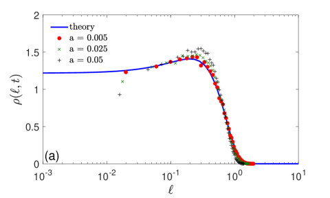
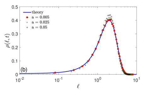
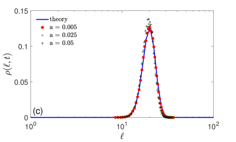
Figure 4: Probability density function $\rho(\ell,t)$ of the boundary local time $\ell_{t}$ for a disk of radius $R=1$, with $D=1$ and three values of time: (a) $t=0.1$, (b) $t=1$, and (c) $t=10$. Solid line shows numerical inversion of the Laplace transform in Eq. (94), whereas symbols illustrate normalized histograms obtained from Monte Carlo simulations, with $M=10^{5}$, $\delta=10^{-5}$, and three values of $a$ as indicated in the legend.

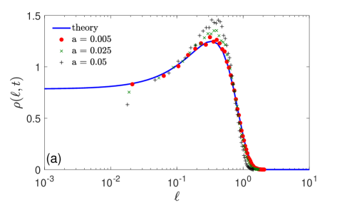
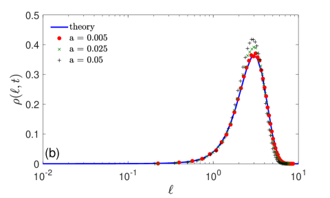
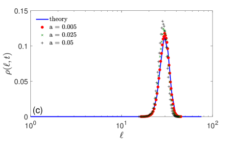
Figure 5: Probability density function $\rho(\ell,t)$ of the boundary local time $\ell_{t}$ for a ball of radius $R=1$, with $D=1$ and three values of time: (a) $t=0.1$. (b) $t=1$, and (c) $t=10$. Solid line shows numerical inversion of the Laplace transform in Eq. (94), whereas symbols illustrate normalized histograms obtained from Monte Carlo simulations, with $M=10^{5}$, $\delta=10^{-5}$, and three values of $a$ indicated in the legend.

References

- (1) S. Redner, A Guide to First Passage Processes (Cambridge: Cambridge University press, 2001).
- (2) Z. Schuss, Brownian Dynamics at Boundaries and Interfaces in Physics, Chemistry and Biology (Springer, New York, 2013).
- (3) R. Metzler, G. Oshanin, and S. Redner (Eds.) First-Passage Phenomena and Their Applications (Singapore: World Scientific, 2014).
- (4) G. Oshanin, R. Metzler, K. Lindenberg (Eds.) Chemical Kinetics: Beyond the Textbook (World Scientific, 2019).
- (5) J.-P. Bouchaud and A. Georges, “Anomalous diffusion in disordered media: Statistical mechanisms, models and physical applications” Phys. Rep. 195, 127-293 (1990).
- (6) D. S. Grebenkov, “NMR Survey of Reflected Brownian Motion”, Rev. Mod. Phys. 79, 1077-1137 (2007).
- (7) O. Bénichou and R. Voituriez, “From first-passage times of random walks in confinement to geometry-controlled kinetics”, Phys. Rep. 539, 225-284 (2014).
- (8) K. Ito and H. P. McKean, Diffusion Processes and Their Sample Paths (Springer-Verlag, Berlin, 1965).
- (9) M. Freidlin, Functional Integration and Partial Differential Equations (Annals of Mathematics Studies, Princeton University Press, Princeton, New Jersey, 1985).
- (10) R. F. Anderson and S. Orey, “Small Random Perturbations of Dynamical Systems with Reflecting Boundary”, Nagoya Math. J. 60, 189-216 (1976).
- (11) G. A. Brosamler, “A probabilistic solution of the Neumann problem”, Math. Scand. 38, 137-147 (1976).
- (12) P. L. Lions and A. S. Sznitman, “Stochastic Differential Equations with Reflecting Boundary Conditions”, Comm. Pure Appl. Math. 37, 511-537 (1984).
- (13) Y. Saisho, “Stochastic Differential Equations for Multi-Dimentional Domain with Reflecting Boundary”, Probab. Theory Rel. Fields 74, 455-477 (1987).
- (14) E. Hsu, “Probabilistic approach to the Neumann problem”, Comm. Pure Appl. Math. 38, 445-472 (1985).
- (15) R. J. Williams, “Local Time and Excursions of Reflected Brownian Motion in a Wedge”, Publ. RIMS 23, 297-319 (1987).
- (16) P. Lévy, Processus Stochastiques et Mouvement Brownien (Paris, Gauthier-Villard, 1948-1965).
- (17) D. A. Lauffenburger and J. Linderman, Receptors: Models for Binding, Trafficking, and Signaling (Oxford University Press, 1993).
- (18) D. Shoup and A. Szabo, “Role of diffusion in ligand binding to macromolecules and cell-bound receptors”, Biophys. J. 40, 33-39 (1982).
- (19) B. Sapoval, “General Formulation of Laplacian Transfer Across Irregular Surfaces”, Phys. Rev. Lett. 73, 3314-3317 (1994).
- (20) B. Sapoval, M. Filoche, and E. Weibel, “Smaller is better – but not too small: A physical scale for the design of the mammalian pulmonary acinus”, Proc. Nat. Ac. Sci. USA 99, 10411-10416 (2002).
- (21) D. S. Grebenkov, M. Filoche, B. Sapoval, and M. Felici, “Diffusion-Reaction in Branched Structures: Theory and Application to the Lung Acinus”, Phys. Rev. Lett. 94, 050602 (2005).
- (22) P. Levitz, D. S. Grebenkov, M. Zinsmeister, K. Kolwankar, and B. Sapoval, “Brownian flights over a fractal nest and first passage statistics on irregular surfaces”, Phys. Rev. Lett. 96, 180601 (2006).
- (23) P. Levitz, M. Zinsmeister, P. Davidson, D. Constantin, and O. Poncelet, “Intermittent Brownian dynamics over a rigid strand: Heavily tailed relocation statistics”, Phys. Rev. E 78, 030102(R) (2008).
- (24) O. Bénichou, D. S. Grebenkov, P. Levitz, C. Loverdo, and R. Voituriez, “Optimal Reaction Time for Surface-Mediated Diffusion”, Phys. Rev. Lett. 105, 150606 (2010).
- (25) O. Bénichou, C. Chevalier, J. Klafter, B. Meyer, and R. Voituriez, “Geometry-controlled kinetics”, Nature Chem. 2, 472-477 (2010).
- (26) F. Rojo, C. E. Budde Jr., H. S. Wio, and C. E. Budde, “Enhanced transport through desorption-mediated diffusion”, Phys. Rev. E 87, 012115 (2013).
- (27) P. C. Bressloff and J. M. Newby, “Stochastic models of intracellular transport”, Rev. Mod. Phys. 85, 135-196 (2013).
- (28) D. S. Grebenkov, “Imperfect Diffusion-Controlled Reactions”, in Chemical Kinetics: Beyond the Textbook, Eds. K. Lindenberg, R. Metzler, and G. Oshanin (World Scientific, 2019).
- (29) D. S. Grebenkov, Partially Reflected Brownian Motion: A Stochastic Approach to Transport Phenomena, in “Focus on Probability Theory”, Ed. L. R. Velle, pp. 135-169 (Nova Science Publishers, 2006).
- (30) D. S. Grebenkov, “Residence times and other functionals of reflected Brownian motion”, Phys. Rev. E 76, 041139 (2007).
- (31) D. S. Grebenkov, “Laplacian Eigenfunctions in NMR. II Theoretical Advances”, Conc. Magn. Reson. 34A, 264-296 (2009).
- (32) A. N. Borodin and P. Salminen, Handbook of Brownian Motion: Facts and Formulae (Birkhauser Verlag, Basel-Boston-Berlin, 1996).
- (33) L. Takacs, “On the Local Time of the Brownian Motion”, Ann. Appl. Probab. 5, 741-756 (1995).
- (34) J. Randon-Furling and S. Redner, “Residence time near an absorbing set”, J. Stat. Mech. 103205 (2018).
- (35) D. A. Darling and M. Kac, “On Occupation Times of the Markoff Processes”, Trans. Am. Math. Soc. 84, 444-458 (1957).
- (36) N. Agmon, “Residence times in diffusion processes”, J. Chem. Phys. 81, 3644-3647 (1984).
- (37) A. M. Berezhkovskii, V. Zaloj, and N. Agmon, “Residence time distribution of a Brownian particle”, Phys. Rev. E 57, 3937-3947 (1998).
- (38) S. N. Majumdar, “Brownian functionals in Physics and Computer Science”, Curr. Sci. 89, 2076-2092 (2005).
- (39) O. Bénichou, M. Coppey, M. Moreau, P. H. Suet, and R. Voituriez, “Averaged residence times of stochastic motions in bounded domains”, Euro. Phys. Lett. 70, 42-48 (2005).
- (40) S. Condamin, O. Bénichou, and M. Moreau, “First-exit times and residence times for discrete random walks on finite lattices”, Phys. Rev. E 72, 016127 (2005).
- (41) S. Condamin, V. Tejedor, and O. Bénichou, “Occupation times of random walks in confined geometries: From random trap model to diffusion-limited reactions”, Phys. Rev. E 76, 050102R (2007).
- (42) B.-T. Nguyen and D. S. Grebenkov, “A Spectral Approach to Survival Probabilities in Porous Media”, J. Stat. Phys. 141, 532-554 (2010).
- (43) D. S. Grebenkov, “Spectral theory of imperfect diffusion-controlled reactions on heterogeneous catalytic surfaces”, J. Chem. Phys. 151, 104108 (2019).
- (44) V. G. Papanicolaou, “The probabilistic solution of the third boundary value problem for second order elliptic equations”, Probab. Th. Rel. Fields 87, 27-77 (1990).
- (45) R. F. Bass, K. Burdzy, and Z.-Q. Chen, “On the Robin problem in Fractal Domains”, Proc. London Math. Soc. 96, 273-311 (2008).
- (46) Y. Zhou and W. Cai, “Numerical Solution of the Robin Problem of Laplace Equations with a Feynman-Kac Formula and Reflecting Brownian Motions”, J. Scient. Comput. 69, 107-121 (2016).
- (47) F. C. Collins and G. E. Kimball, “Diffusion-controlled reaction rates”, J. Coll. Sci. 4, 425 (1949).
- (48) H. Sano and M. Tachiya, “Partially diffusion-controlled recombination”, J. Chem. Phys. 71, 1276-1282 (1979).
- (49) H. Sano and M. Tachiya, “Theory of diffusion-controlled reactions on spherical surfaces and its application to reactions on micellar surfaces”, J. Chem. Phys. 75, 2870-2878 (1981).
- (50) O. Bénichou, M. Moreau, and G. Oshanin, “Kinetics of stochastically gated diffusion-limited reactions and geometry of random walk trajectories”, Phys. Rev. E 61, 3388 (2000).
- (51) D. S. Grebenkov, M. Filoche, and B. Sapoval, “Mathematical Basis for a General Theory of Laplacian Transport towards Irregular Interfaces”, Phys. Rev. E 73, 021103 (2006).
- (52) P. C. Bressloff, B. A. Earnshaw, and M. J. Ward, “Diffusion of protein receptors on a cylindrical dendritic membrane with partially absorbing traps”, SIAM J. Appl. Math. 68, 1223 (2008).
- (53) A. Singer, Z. Schuss, A. Osipov, and D. Holcman, “Partially reflected diffusion”, SIAM J. Appl. Math. 68, 844-868 (2008).
- (54) D. S. Grebenkov, “Searching for partially reactive sites: Analytical results for spherical targets”, J. Chem. Phys. 132, 034104 (2010).
- (55) D. S. Grebenkov, “Subdiffusion in a bounded domain with a partially absorbing-reflecting boundary”, Phys. Rev. E 81, 021128 (2010).
- (56) F. Rojo, H. S. Wio, and C. E. Budde, “Narrow-escape-time problem: The imperfect trapping case”, Phys. Rev. E 86, 031105 (2012).
- (57) D. S. Grebenkov, “Analytical representations of the spread harmonic measure density”, Phys. Rev. E 91, 052108 (2015).
- (58) R. Zwanzig, “Diffusion-controlled ligand binding to spheres partially covered by receptors: an effective medium treatment”, Proc. Natl. Acad. Sci. USA 87, 5856 (1990).
- (59) A. Berezhkovskii, Y. Makhnovskii, M. Monine, V. Zitserman, and S. Shvartsman, “Boundary homogenization for trapping by patchy surfaces”, J. Chem. Phys. 121, 11390 (2004).
- (60) A. M. Berezhkovskii, M. I. Monine, C. B. Muratov, and S. Y. Shvartsman, “Homogenization of boundary conditions for surfaces with regular arrays of traps”, J. Chem. Phys. 124, 036103 (2006).
- (61) C. Muratov and S. Shvartsman, “Boundary homogenization for periodic arrays of absorbers”, Multiscale Model. Simul. 7, 44-61 (2008).
- (62) L. Dagdug, M. Vázquez, A. Berezhkovskii, and V. Zitserman, “Boundary homogenization for a sphere with an absorbing cap of arbitrary size”, J. Chem. Phys. 145, 214101 (2016).
- (63) A. Bernoff, A. Lindsay, and D. Schmidt, “Boundary Homogenization and Capture Time Distributions of Semipermeable Membranes with Periodic Patterns of Reactive Sites”, Multiscale Model. Simul. 16, 1411-1447 (2018).
- (64) M. Filoche and B. Sapoval, “Can One Hear the Shape of an Electrode? II. Theoretical Study of the Laplacian Transfer”, Eur. Phys. J. B 9, 755-763 (1999).
- (65) D. S. Grebenkov, M. Filoche, and B. Sapoval, “Spectral Properties of the Brownian Self-Transport Operator”, Eur. Phys. J. B 36, 221-231 (2003).
- (66) C. W. Gardiner, Handbook of stochastic methods for physics, chemistry and the natural sciences (Springer: Berlin, 1985).
- (67) Yu. Egorov, Pseudo-differential Operators, Singularities, Applications (Berlin: Birkhauser, Basel, Boston, 1997).
- (68) N. Jacob, Pseudo-differential Operators and Markov Processes (Berlin: Akademie-Verlag, 1996).
- (69) M. E. Taylor, Pseudodifferential Operators (Princeton, New Jersey: Prince-ton University Press, 1981).
- (70) M. Marletta, “Eigenvalue problems on exterior domains and Dirichlet to Neumann maps”, J. Comput. Appl. Math. 171, 367-391 (2004).
- (71) W. Arendt, R. Mazzeo, “Spectral properties of the Dirichlet-to-Neumann operator on Lipschitz domains”, Ulmer Seminare 12, 23-37 (2007).
- (72) W. Arendt and A. F. M. ter Elst, “The Dirichlet-to-Neumann Operator on Exterior Domains”, Potential Anal. 43, 313-340 (2015).
- (73) A. Hassell and V. Ivrii, “Spectral asymptotics for the semiclassical Dirichlet to Neumann operator”, J. Spectr. Theory 7, 881-905 (2017).
- (74) A. Girouard and I. Polterovich, “Spectral geometry of the Steklov problem”, J. Spectr. Theory 7, 321-359 (2017).
- (75) S. B. Yuste, E. Abad, and K. Lindenberg, “Exploration and trapping of mortal random walkers”, Phys. Rev. Lett. 110, 220603 (2013).
- (76) B. Meerson and S. Redner, “Mortality, redundancy, and diversity in stochastic search”, Phys. Rev. Lett. 114, 198101 (2015).
- (77) D. S. Grebenkov and J.-F. Rupprecht, “The escape problem for mortal walkers”, J. Chem. Phys. 146, 084106 (2017).
- (78) D. S. Grebenkov and B.-T. Nguyen, “Geometrical structure of Laplacian eigenfunctions”, SIAM Rev. 55, 601-667 (2013).
- (79) J. P. Morillon, “Numerical solutions of linear mixed boundary value problems using stochastic representations”, Int. J. Numer. Meth. Engng. 40, 387-405 (1997).
- (80) C. Costantini, B. Pacchiarotti, and F. Sartoretto, “Numerical approximation for functionals of reflecting diffusion processes”, SIAM J. Appl. Math. 58, 73-102 (1998).
- (81) D. S. Grebenkov, “Efficient Monte Carlo methods for simulating diffusion-reaction processes in complex systems”, in First-Passage Phenomena and Their Applications, Eds. R. Metzler, G. Oshanin, S. Redner (World Scientific Press, 2014).
- (82) Y. Zhou, W. Cai, and E. Hsu, “Computation of the local time of reflecting Brownian motion and the probabilistic representation of the Neumann problem”, Comm. Math. Sci. 15, 237-259 (2017).