Three-in-a-Tree in Near Linear Time

Abstract

The three-in-a-tree problem is to determine if a simple undirected graph contains an induced subgraph which is a tree connecting three given vertices. Based on a beautiful characterization that is proved in more than twenty pages, Chudnovsky and Seymour [Combinatorica 2010] gave the previously only known polynomial-time algorithm, running in $O(mn^{2})$ time, to solve the three-in-a-tree problem on an $n$-vertex $m$-edge graph. Their three-in-a-tree algorithm has become a critical subroutine in several state-of-the-art graph recognition and detection algorithms.

In this paper we solve the three-in-a-tree problem in $\tilde{O}(m)$ time, leading to improved algorithms for recognizing perfect graphs and detecting thetas, pyramids, beetles, and odd and even holes. Our result is based on a new and more constructive characterization than that of Chudnovsky and Seymour. Our new characterization is stronger than the original, and our proof implies a new simpler proof for the original characterization. The improved characterization gains the first factor $n$ in speed. The remaining improvement is based on dynamic graph algorithms.

1 Introduction

The graphs considered in this paper are all assumed to be undirected. Also, it is convenient to think of them as connected. Let $G$ be such a graph with $n$ vertices and $m$ edges. An induced subgraph of $G$ is a subgraph $H$ that contains all edges from $G$ between vertices in $H$. For the three-in-a-tree problem, we are given three specific terminals in $G$, and we want to decide if $G$ has an induced tree $T$, that is, a tree $T$ which is an induced subgraph of $G$, containing these terminals. Chudnovsky and Seymour [28] gave the formerly only known polynomial-time algorithm, running in $O(mn^{2})$ time, for the three-in-a-tree problem. In this paper, we reduce the complexity of three-in-a-tree from $O(mn^{2})$ to $O(m\log^{2}n)=\tilde{O}(m)$ time.

Theorem 1.1.

It takes $O(m\log^{2}n)$ time to solve the three-in-a-tree problem on an $n$-vertex $m$-edge simple graph.

To prove Theorem 1.1, we first improve the running time to $O(mn)$ using a simpler algorithm with a simpler correctness proof than that of Chudnovsky and Seymour. The remaining improvement is done employing dynamic graph algorithms.

1.1 Significance of three-in-a-tree

The three-in-a-tree problem may seem like a toy problem, but it has proven to be of general importance because many difficult graph detection and recognition problems reduce to it. The reductions are often highly non-trivial and one-to-many, solving three-in-a-tree on multiple graph instances with different placements of the three terminals. With our near-linear three-in-a-tree algorithm and some improved reductions, we get the results summarized Figure 1. These results will be explained in more detail in Section 1.2.

best previously known results our work three-in-a-tree $O(n^{4})$ [28] $\tilde{O}(n^{2})$: Theorem 1.1 theta $O(n^{11})$ [28] $\tilde{O}(n^{6})$: Theorem 1.2 pyramid $O(n^{9})$ [18] $\tilde{O}(n^{5})$: Theorem 1.3 perfect graph $O(n^{9})$ [18] $O(n^{8})$: Theorem 1.4 odd hole $O(n^{9})$ [26] $O(n^{8})$: Theorem 1.4 beetle $O(n^{11})$ [15] $\tilde{O}(n^{6})$: Theorem 1.5 even hole $O(n^{11})$ [15] $O(n^{9})$: Theorem 1.6

Figure 1: Comparing our work with the best previously known results for an $n$-vertex graph.

Showcasing some of the connections, our improved three-in-a-tree algorithm leads to an improved algorithm to detect if a graph has an odd hole, that is, an induced cycle of odd length above three. This is via the recent odd-hole algorithm of Chudnovsky, Scott, Seymour, and Spirkl [26]. A highly nontrivial consequence of odd-hole algorithm is that we can use it to recognize if a graph $G$ is perfect, that is, if the chromatic number of each induced subgraph $H$ of $G$ equals the clique number of $H$. The celebrated Strong Perfect Graph Theorem states that a graph is perfect if and only if neither the graph nor its complement has an odd hole. An odd-hole algorithm can therefore trivially test if a graph is perfect. The Strong Perfect Graph Theorem, implying the last reduction was a big challenge to mathematics, conjectured by Berge in 1960 [6, 7, 8] and proved by Chudnovsky, Robertson, Seymour, and Thomas [25], earned them the 2009 Fulkerson prize. Our improved three-in-a-tree algorithm improves the time to recognize if a graph is perfect from $O(n^{9})$ to $O(n^{8})$. While this is a modest polynomial improvement, the point is that three-in-a-tree is a central sub-problem on the path to solve many other problems.

The next obvious question is why three-in-a-tree? Couldn’t we have found a more general subproblem to reduce to? The dream would be to get something like disjoint paths and graph minor theory where we detect a constant sized minor or detect if we have disjoint paths connecting of a constant number of terminal pairs (one path connecting each pair) in $O(n^{2})$ time. This is using the algorithm of Kawarabayashi, Kobayashi, and Reed [61], improving the original cubic algorithm of Robertson and Seymour [71].

In light of the above grand achievements, it may seem unambitious for Chudnovsky and Seymour to work on three-in-a-tree as a general tool. The difference is that the above disjoint paths and minors are not necessarily induced subgraphs. Working with induced paths, many of the most basic problems become NP-hard. Obviously, we can decide if there is an induced path between two terminals, but Bienstock [9] has proven that it is NP-hard to decide two-in-a-cycle, that is, if two terminals are in an induced cycle. From this we easily get that it is NP-hard to decide three-in-a-path, that is if there is an induced path containing three given terminals. Both of these problems would be trivial if we could solve the induced disjoint path problem for just two terminal pairs. In connection with the even and odd holes and perfect graphs, Bienstock also proved that it is NP-hard to decide if there is an even (respectively, odd) hole containing a given terminal.

In light of these NP-hardness results it appears quite lucky that three-in-a-tree is tractable, and of sufficient generality that it can be used as a base for solving other graph detection and recognition problems nestled between NP-hard problems. In fact, three-in-a-tree has become such a dominant tool in graph detection that authors sometimes explained when they think it cannot be used [29, 78], e.g., Trotignon and Vušković [78] wrote “A very powerful tool for solving detection problems is the algorithm three-in-a-tree of Chudnovsky and Seymour […] But as far as we can see, three-in-a-tree cannot be used to solve $\Pi_{H_{1|1}}$.”

While proving that a problem is in P is the first big step in understanding the complexity, there has also been substantial prior work on improving the polynomial complexity for many of the problems considered in this paper. In the next subsection, we will explain in more detail how our near-linear three-in-a-tree algorithm together with some new reductions improve the complexity of different graph detection and recognition problems. In doing so we also hope to inspire more new applications of three-in-a-tree in efficient graph algorithms.

1.2 Implications

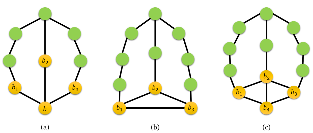
Figure 2: (a) Theta. (b) Pyramid. (c) Beetle.

We are now going to describe the use of our three-in-a-tree algorithm to improve the complexity of several graph detection and recognition problems. The reader less familiar with structural graph theory may find it interesting to see how the route to solve the big problems takes us through several toy-like subproblems, starting from three-in-a-tree. Often we look for some simple configuration implying an easy answer. If the simple configuration is not present, then this tells us something about the structure of the graph that we can try to exploit.

We first define the big problems in context. A hole is an induced simple cycle with four or more vertices. A graph is chordal if and only if it has no hole. Rose, Tarjan, and Leuker [72] gave a linear-time algorithm for recognizing chordal graphs. A hole is odd (respectively, even) if it consists of an odd (respectively, even) number of vertices. $G$ is Berge if $G$ and its complement are both odd-hole-free. The celebrated Strong Perfect Graph Theorem, which was conjectured by Berge [6, 7, 8] and proved by Chudnovsky, Robertson, Seymour, and Thomas [25], states that $G$ is Berge if and only if $G$ is perfect, i.e., the chromatic number of each induced subgraph $H$ of $G$ equals the clique number of $H$.

The big problems considered here are the detection of odd and even holes, but related to this we are going to look for “thetas”, “pyramids”, and “beetles”, as illustrated in Figure 2. These are different induced subdivisions where a subdivision of a graph is one where edges are replaced by paths of arbitrary length. A hole is thus an induced subdivision of a length-4 cycle, and a minimal three-in-a-tree is an induced subdivision of a star with two or three leaves that are all prespecified terminals.

The first problem Chudnovsky and Seymour [28] solved using their three-in-tree algorithm was to detect a theta which is any induced subdivision of $K_{2,3}$ [5]. Chudnovsky and Seymour are interested in thetas because they trivially imply an even hole. They developed the previously only known polynomial-time algorithm, running in $O(n^{11})$ time, for detecting thetas in $G$ via solving the three-in-a-tree problem on $O(n^{7})$ subgraphs of $G$. Thus, Theorem 1.1 reduces the time to $\tilde{O}(n^{9})$. Moreover, we show in Lemma 6.1 that thetas in $G$ can be detected via solving the three-in-a-tree problem on $O(mn^{2})$ $n$-vertex graphs, leading to an $\tilde{O}(n^{6})$-time algorithm as stated in Theorem 1.2.

Theorem 1.2.

It takes $O(mn^{4}\log^{2}n)$ time to detect thetas in an $n$-vertex $m$-edge graph.

The next problem Chudnovsky and Seymour solved using their three-in-tree algorithm was to detect a pyramid which is an induced subgraph consisting of an apex vertex $u$ and a triangle $v_{1}v_{2}v_{3}$ and three paths $P_{1}$, $P_{2}$, and $P_{3}$ such that $P_{i}$ connects $u$ to $v_{i}$ and touch $P_{j}$, $j\neq i$, only in $u$, and such that at most one of $P_{1}$, $P_{2}$, and $P_{3}$ has only one edge. The point in a pyramid is that it must contain an odd hole. An $O(n^{9})$-time algorithm for detecting pyramids was already contained in the perfect graph algorithm of Chudnovsky et al. [18, §2], but Chudnovsky and Seymour use their three-in-a-tree to give a more natural “less miraculous” algorithm for pyramid detection, but with a slower running time of $O(n^{10})$. With our faster three-in-a-tree algorithm, their more natural pyramid detection also becomes the faster algorithm with a running time of $\tilde{O}(n^{8})$. Moreover, as for thetas, we improve the reductions to three-in-a-tree. We show (see Lemma 6.2) that pyramids in $G$ can be detected via solving the three-in-a-tree problem on $O(mn)$ $n$-vertex graphs, leading to an $\tilde{O}(mn^{3})$-time algorithm as stated in Theorem 1.3.

Theorem 1.3.

It takes $O(mn^{3}\log^{2}n)$ time to detect pyramids in an $n$-vertex $m$-edge graph.

We now turn to odd holes and perfect graphs. Since a graph is perfect if and only if it and its complement are both odd-hole-free, an odd-hole algorithm implies a perfect graph algorithm, but not vice versa. Cornuéjols, Liu, and Vušković [39] gave a decomposition-based algorithm for recognizing perfect graphs that runs in $O(n^{18})$ time, which was reduced to $O(n^{15})$ time by Charbit, Habib, Trotignon, and Vušković [17]. The best previously known algorithm, due to Chudnovsky, Cornuéjols, Liu, Seymour, and Vušković [18], runs in $O(n^{9})$ time. However, the tractability of detecting odd holes was open for decades [30, 33, 37, 59] until recently. Chudnovsky, Scott, Seymour, and Spirkl [26] announced an $O(n^{9})$-time algorithm for detecting odd holes, which also implies a simpler $O(n^{9})$-time algorithm for recognizing perfect graphs. An $O(n^{9})$-time bottleneck of both of these perfect-graph recognition algorithms was the above mentioned algorithm for detecting pyramids [18, §2].

By Theorem 1.3, the pyramids can now be detected in $\tilde{O}(mn^{3})$-time, but Chudnovsky et al.’s odd-hole algorithm has six more $O(n^{9})$-time subroutines [26, §4]. By improving all these bottle-neck subroutines, we improve the detection time for odd holes to $O(m^{2}n^{4})$, hence the recognition time for perfect graphs to $O(n^{8})$.

Theorem 1.4.

(1) It takes $O(m^{2}n^{4})$ time to detect odd holes in an $n$-vertex $m$-edge graph, and hence (2) it takes $O(n^{8})$ time to recognize an $n$-vertex perfect graph.

Even-hole-free graphs have been extensively studied [2, 34, 35, 40, 41, 52, 62, 74]. Vušković [83] gave a comprehensive survey. Conforti, Cornuéjols, Kapoor, and Vušković [32, 36] gave the first polynomial-time algorithm for detecting even holes, running in $O(n^{40})$ time. Chudnovsky, Kawarabayashi, and Seymour [20] reduced the time to $O(n^{31})$. A prism consists of two vertex-disjoint triangles together with three vertex-disjoint paths between the two triangles such that the union of every two of the three paths induces a cycle. Chudnovsky et al. [20] also observed that the time of detecting even holes can be further reduced to $O(n^{15})$ as long as detecting prisms is not too expensive, but this turned out to be NP-hard [68]. However, Chudnovsky and Kapadia [19] and Maffray and Trotignon [68, Algorithm 2] devised $O(n^{35})$-time and $O(n^{5})$-time algorithms for detecting prisms in theta-free and pyramid-free graphs $G$, respectively. Later, da Silva and Vušković [41] improved the time of detecting even holes in $G$ to $O(n^{19})$. The best formerly known algorithm, due to Chang and Lu [15], runs in $O(n^{11})$ time. One of its two $O(n^{11})$-time bottlenecks [15, Lemma 2.3] detects so-called beetles in $G$ via solving the three-in-a-tree problem on $O(n^{7})$ subgraphs of $G$. Theorem 1.1 reduces the time to $\tilde{O}(n^{9})$. Moreover, we show in Lemma 6.3 that beetles can be detected via solving the three-in-a-tree problem on $O(m^{2})$ $n$-vertex graphs, leading to an $\tilde{O}(n^{6})$-time algorithm as stated in Theorem 1.5.

Theorem 1.5.

It takes $O(m^{2}n^{2}\log^{2}n)$ time to detect beetles in an $n$-vertex $m$-edge graph.

Combining our faster beetle-detection algorithm with our $O(n^{9})$-time algorithm in §6.3, which is carefully improved from the other $O(n^{11})$-time bottleneck subroutine [15, Lemma 2.4], we reduce the time of detecting even holes to $O(n^{9})$ as stated in Theorem 1.6.

Theorem 1.6.

It takes $O(m^{2}n^{5})$ time to detect even holes in an $n$-vertex $m$-edge graph.

For other implications of Theorem 1.1, Lévêque, Lin, Maffray, and Trotignon gave $O(n^{13})$-time and $O(n^{14})$-time algorithms for certain properties $\Pi_{B_{4}}$ and $\Pi_{B_{6}}$, respectively [66, Theorems 3.1 and 3.2]. By Theorem 1.1 and the technique of §6.2.1, the time can be reduced by a $\Theta({n^{5}}/{\log^{2}n})$ factor. Theorem 1.1 also improves the algorithms of van ’t Hof, Kaminski, and Paulusma [81, Lemmas 4 and 5]. We hope and expect that three-in-a-tree with its new near-optimal efficiency will find many other applications in efficient graph algorithms.

1.3 Other related work

For the general $k$-in-a-tree problem, we are given $k$ specific terminals in $G$, and we want to decide if $G$ has an induced tree $T$. The $k$-in-a-tree problem is NP-complete [43] when $k$ is not fixed. With our Theorem 1.1, it can be solved in near-linear time for $k\leq 3$, and the tractability is unknown for any fixed $k\geq 4$ [54]. Solving it in polynomial time for constant $k$ would be a huge result. It is, however, not clear that $k$-in-a-tree for $k>3$ would be as powerful a tool in solving other problems as three-in-a-tree has proven to be.

While $k$-in-a-tree with bounded $k$ is unsolved for general graphs, there has been substantial work devoted to $k$-in-a-tree for special graph classes. Derhy, Picouleau, and Trotignon [44] and Liu and Trotignon [67] studied $k$-in-a-tree on graphs with girth at least $k$ for $k=4$ and general $k\geq 4$, respectively. Dos Santos, da Silva, and Szwarcfiter [48] studied the $k$-in-a-tree problem on chordal graphs. Golovach, Paulusma, and van Leeuwen [54] studied the $k$-in-a-tree, $k$-in-a-cycle, and $k$-in-a-path problems on AT-free graphs [65]. Bruhn and Saito [13], Fiala, Kaminski, Lidický, and Paulusma [50], and Golovach, Paulusma, and van Leeuwen [55] studied the $k$-in-a-tree and $k$-in-a-path problems on claw-free graphs.

See [1, 4, 11, 14, 16, 21, 22, 23, 24, 27, 37, 46, 47, 49, 51, 53, 57, 70, 73] for more work on graph detection, recognition, and characterization. Also see [12, Appendix A] for a survey of the recognition complexity of more than $160$ graph classes.

On the hardness side, recall that three-in-a-tree can also be viewed as three in a subdivided star with two or three terminal leaves. However, detecting such a star with 4 terminal leaves is NP-hard. (This follows from Bienstock’s NP-hardness of 2-in-a-cycle [9], asking if there exists a hole containing two vertices $u$ and $v$, which may be assumed to be nonadjacent: Add two new leaves $u_{1}$ and $u_{2}$ adjacent to $u$ and then, for every two neighbors $v_{1}$ and $v_{2}$ of $v$, check if the new graph contains an induced subdivision of a star with exactly four terminal leaves $u_{1},u_{2},v_{1},v_{2}$.) Even without terminals, it is NP-hard to detect induced subdivisions of any graph with minimum degree at least four [4, 66]. Finally, we note that if we allow multigraphs with parallel edges, then even 2-in-a-path becomes NP-hard. This NP-hardness is an easy exercise since the induced path cannot contain both end-points of parallel edges.

We note that it is the subdivisions that make induced graph detection hard for constant sized pattern graphs. Without subdivisions, we can trivially check for any induced $k$-vertex graph in $O(n^{k})$ time. Nesetril and Poljak has improved this to roughly $O(n^{k\omega/3})$ where $\omega$ is the exponent of matrix multiplication [69]. On the other hand, the ETH hypothesis implies that we cannot detect if a $k$-clique is a(n induced) subgraph in $n^{o(k)}$ time [60]. A more general understanding of the hardness of detecting induced graphs has been presented recently in [42].

1.4 Techniques

Chudnovsky and Seymour’s $O(n^{2}m)$-time algorithm for the three-in-a-tree problem is based upon their beautiful characterization for when a graph with three given terminals are contained in some induced tree [28]. The aim is to either find a three-in-a-tree or a witness that it cannot exist. During the course of the algorithm, they develop the witness to cover more and more of the graph. In each iteration, they take some part that is not covered by the current witness and try to add it in, but then some other part of the witness may pop out. They then need a potential function argument to show progress in each iteration.

What we do is to introduce some extra structure to the witness when no three-in-a-tree is found, so that when things are added, nothing pops out. This leads to a simpler more constructive algorithm that is faster by a factor $n$. Our new witness has more properties than that of Chudnovsky and Seymour, so our characterization of no three-in-a-tree is strictly stronger, yet our overall proof is shorter. Essentially the point is that by strengthening the inductive hypothesis, we get a simpler inductive step. The remaining improvement in speed is based on dynamic graph algorithms.

1.5 Road map

The rest of the paper is organized as follows. Section 2 is a background section where we review Chudnovsky and Seymour’s characterization for three-in-a-tree, sketch how it is used algorithmically, as well as the bottleneck for a fast implementation. Section 3 presents our new stronger characterization as well as a high level description of the algorithms and proofs leading to our $\tilde{O}(m)$ implementation. Section 4 proves the correctness of our new characterization. Section 5 provides an efficient implementation. Finally, Section 6 shows how our improved three-in-a-tree algorithm, in tandem with other new ideas, can be used to improve many state-of-the-art graph recognition and detection algorithms. Section 7 concludes the paper.

2 Background

2.1 Preliminaries

Let $|S|$ denote the cardinality of set $S$. Let $R\setminus S$ for sets $R$ and $S$ consist of the elements of $R$ not in $S$. Let $G$ and $H$ be graphs. Let $V(G)$ (respectively, $E(G)$) consist of the vertices (respectively, edges) of $G$. Let $u$ and $v$ be vertices. Let $U$ and $V$ be vertex sets. Let $N_{G}(u)$ consist of the neighbors of $u$ in $G$. The degree of $u$ in $G$ is $|N_{G}(u)|$. Let $N_{G}[u]=N_{G}(u)\cup\{u\}$. Let $N_{G}(U)$ be the union of $N_{G}(u)\setminus U$ over all vertices $u\in U$. Let $N_{G}(u,H)=N_{G}(u)\cap V(H)$ and $N_{G}(U,H)=N_{G}(U)\cap V(H)$. The subscript $G$ in notation $N_{G}$ may be omitted. A leaf of $G$ is a degree-one vertex of $G$. Let $\nabla(G)$ denote the graph obtained from $G$ by adding an edge between each pair of leaves of $G$. Let $G[H]$ denote the subgraph of $G$ induced by $V(H)$. Let $G-U=G[V(G)\setminus U]$. Let $G-u=G-\{u\}$. Let $uv$ denote an edge with end-vertices $u$ and $v$. Graphs $H_{1}$ and $H_{2}$ are disjoint if $V(H_{1})\cap V(H_{2})=\varnothing$. Graphs $H_{1}$ and $H_{2}$ are adjacent in $G$ if $H_{1}$ and $H_{2}$ are disjoint and there is an edge $uv$ of $G$ with $u\in V(H_{1})$ and $v\in V(H_{2})$. A $UV$-path is either a vertex in $U\cap V$ or a path having one end-vertex in $U$ and the other end-vertex in $V$. A $UV$-rung [28] is a vertex-minimal induced $UV$-path. If $U=\{u\}$, then a $UV$-path is also called a $uV$-path and a $Vu$-path. If $U=\{u\}$ and $V=\{v\}$, then a $UV$-path is also called a $uv$-path. Let $Uv$-rung, $uV$-rung, and $uv$-rung be defined similarly.

For the three-in-a-tree problem, we assume without loss of generality that the three given terminals of the input $n$-vertex $m$-edge simple undirected graph $G$ are exactly the leaves of $G$. A sapling of $G$ is an induced tree containing all three leaves of $G$, so the three-in-a-tree problem is the problem of finding a sapling.

2.2 Chudnovsky and Seymour’s characterization

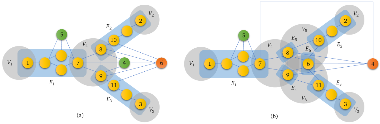
Figure 3: (a) An $X$-net $\mathds{H}$ with nodes $V_{1},\ldots,V_{4}$ and arcs $E_{1},E_{2},E_{3}$, where $X$ consists of the vertices other than $4,5,6$. Vertices $4$ and $5$ are $\mathds{H}$-local. Vertex $6$ is $\mathds{H}$-nonlocal. (b) A nonlocal net $\mathds{H}$ having a triad $\Delta(V_{4},V_{5},V_{6})=\{6,8,9\}$. Vertex $5$ is $\mathds{H}$-local. Vertex $4$ is $\mathds{H}$-nonlocal.

Let $\mathds{H}$ be a graph such that each member of $V(\mathds{H})$ and $E(\mathds{H})$, called node and arc respectively, is a subset of $X\subseteq V(G)$. $\mathds{H}$ is an $X$-net of $G$ if the following Conditions N hold (see Figure 3(a)):

1. 1. Graph $\mathds{H}$ is connected and graph $\nabla(\mathds{H})$ is biconnected.

   2. The arcs of $\mathds{H}$ form a nonempty disjoint partition of the vertex set $X$.

   3. Graph $\mathds{H}$ has exactly three leaf nodes, each of which consists of a leaf vertex of $G$.

   4. For any arc $E=UV$ of $\mathds{H}$, each vertex of $X$ in $E$ is on a $UV$-rung of $G[E]$.

   5. For any arc $E$ and node $V$ of $\mathds{H}$, $E\cap V\neq\varnothing$ if and only if $V$ is an end-node of $E$ in $\mathds{H}$.

   6. For any vertices $u$ and $v$ in $X$ contained by distinct arcs $E$ and $F$ of $\mathds{H}$, $uv$ is an edge of $G$ if and only if arcs $E$ and $F$ share a common end-node $V$ in $\mathds{H}$ with $\{u,v\}\subseteq V$.

An arc $E=UV$ is simple if $G[E]$ is a $UV$-rung. A net is an $X$-net for an $X$. A base net is a net obtained via the next lemma, for which we include a proof to make our paper self-contained.

Lemma 2.1 (Chudnovsky and Seymour [28]).

It takes $O(m)$ time to find a sapling of $G$ or a net of $G$ whose arcs are all simple.

Proof.

Let $s_{1},s_{2},s_{3}$ be the leaves of $G$. Obtain vertex sets $R$ and $S$ such that $G[S]$ is an $s_{2}s_{3}$-rung of $G$ and $G[R]$ is an $s_{1}S$-rung of $G$. Let $x_{1}\in R\setminus S$ be closest to $S$ in $G[R]$. Let each $x_{j}\in N(x_{1},S)$ with $j\in\{2,3\}$ be closest to $s_{j}$ in $G[S]$. Since $s_{2}$ and $s_{3}$ are leaves of $G$, $x_{2}$ and $x_{3}$ are internal vertices of path $G[S]$. If $x_{2}=x_{3}$, then $G[R\cup S]$ is a sapling of $G$. If $x_{2}$ and $x_{3}$ are distinct and nonadjacent, then $G[R\cup S]-I$ is a sapling of $G$, where $I$ consists of the internal vertices of the $x_{2}x_{3}$-path in $G[S]$. If $x_{2}$ and $x_{3}$ are adjacent in $G$, then $G$ admits an $R\cup S$-net having nodes $V_{0}=\{x_{1},x_{2},x_{3}\}$ and $V_{i}=\{s_{i}\}$ with $i\in\{1,2,3\}$ and simple arcs $E_{i}=V_{0}V_{i}$ with $i\in\{1,2,3\}$ consisting of the vertices of the $s_{i}x_{i}$-rung of $G[R\cup S]$. ∎

The original definition of Chudnovsky et al. only used nets with no parallel arcs, but for our own more efficient construction, we need to use parallel arcs. A triad of $\mathds{H}$ is $\Delta(V_{1},V_{2},V_{3})=(V_{1}\cap V_{2})\cup(V_{2}\cap V_{3})\cup(V_{3}\cap V_{1})$ for nodes $V_{1}$, $V_{2}$, and $V_{3}$ that induce a triangle in graph $\mathds{H}$. A subset $S$ of $X$ is $\mathds{H}$-local if $S$ is contained by a node, arc, or triad of $\mathds{H}$ [28]. A set $Y\subseteq V(G-X)$ is $\mathds{H}$-local if $N(Y,X)$ is $\mathds{H}$-local. $\mathds{H}$ is local if every $Y\subseteq V(G-X)$ with connected $G[Y]$ is $\mathds{H}$-local. See Figure 3. The following theorem is Chudnovsky and Seymour’s characterization.

Theorem 2.2 (Chudnovsky and Seymour [28, 3.2]).

$G$ is sapling-free if and only if $G$ admits a local net with no parallel arcs.

The proof of Theorem 2.2 in [28] takes up more than 20 pages. We will here present a stronger characterization with a shorter proof, which moreover leads to a much faster implementation. Our results throughout the paper do not rely on Theorem 2.2. Moreover, our paper delivers an alternative self-contained proof for Theorem 2.2.

Chudnovsky and Seymour’s proof of Theorem 2.2 is algorithmic maintaining an $X$-net $\mathds{H}$ with $X\subseteq V(G)$ having no parallel arcs until a sapling of $G$ is found or $\mathds{H}$ becomes local, implying that $G$ is sapling-free by the if direction of Theorem 2.2. In each iteration, if $\mathds{H}$ is not local, they find a minimal set $Y\subseteq V(G-X)$ with connected $G[Y]$ such that $Y$ is $\mathds{H}$-nonlocal. Their proof for the only-if direction of Theorem 2.2 shows that if $G[X\cup Y]$ is sapling-free, then $\mathds{H}$ can be updated to an $X^{\prime}$-net with $Y\subseteq X^{\prime}\subseteq X\cup Y$. Although $Y$ joins the resulting $X^{\prime}$-net $\mathds{H}$, a subset of $X$ may have to be moved out of $\mathds{H}$ to preserve Conditions N for $\mathds{H}$. To bound the number of iterations, Chudnovsky and Seymour showed that the potential $|X|+(n+1)\cdot|V(\mathds{H})|$ of $\mathds{H}$ stays $O(n^{2})$ and is increased by each iteration, implying that the total number of iterations is $O(n^{2})$. In the next section, we will present a new stronger characterization that using parallel arcs with particular properties avoids the aforementioned in-and-out situation. More precisely, our $X$ will grow in each iteration, reducing the number of iterations to at most $n$.

3 Our stronger characterization

A base net of $G$ contains only simple arcs. However, we do need other more complex arcs, but we will show that it suffices that all non-simple arcs are “flexible” in the sense defined below. For vertex sets $S$, $V_{1}$, and $V_{2}$, an $(S,V_{1},V_{2})$-sprout is an induced subgraph of $G$ in one of the following Types S:

1. 1. A tree intersecting each of $S$, $V_{1}$, and $V_{2}$ at exactly one vertex.

   2. An $SV_{1}$-rung not intersecting $V_{2}$ plus a disjoint $SV_{2}$-rung not intersecting $V_{1}$.

   3. A $V_{1}V_{2}$-rung not intersecting $S$ plus a disjoint $SV$-rung with $V=V_{1}\cup V_{2}$.

Figure 4: A web $\mathds{H}$. The arcs of $\nabla(\mathds{H})$ between the three leaves of $\mathds{H}$ are in yellow.

Let $S=\{1,\ldots,7\}$ for the example in Figure 4. Vertex $1$ is an $(S,V_{1},V_{2})$-sprout of Type SS1. The set $\{2,19,12,11,13,14,15,16\}$ induces an $(S,V_{1},U_{2})$-sprout of Type SS1. The only $(S,U_{1},U_{2})$-sprout and $(S,W_{1},W_{2})$-sprout of Type SS1 contain vertex $1$. The set $\{23,4,7,28\}$ induces an $(S,W_{1},W_{2})$-sprout of Type SS2. The set $\{19,2,13,14,15,16\}$ induces an $(S,U_{1},U_{2})$-sprout of Type SS3. An arc $E=UV$ of $\mathds{H}$ is flexible if $G[E]$ contains an $(S,U,V)$-sprout for each nonempty vertex set $S\subseteq E$. For the example in Figure 4, arcs $E_{1},E_{3},E_{4},E_{5},E_{6}$ are simple and arcs $E_{1},E_{2},E_{7}$ are flexible. An $X$-net $\mathds{H}$ is an $X$-web if all arcs of $\mathds{H}$ are simple or flexible. A web is an $X$-web for some $X$. A base net of $G$ is a web of $G$. Let $\mathds{H}$ be a net. A split component $\mathds{G}$ for $\mathds{H}$ is either an arc $UV$ of $\mathds{H}$ or a subgraph of $\mathds{H}$ containing a cutset $\{U,V\}$ of $\nabla(\mathds{H})$ such that $\mathds{G}$ is a maximal subgraph of $\nabla(\mathds{H})$ in which $U$ and $V$ are nonadjacent and do not form a cutset [45]. For both cases, we call $\{U,V\}$ the split pair of $\mathds{G}$ for $\mathds{H}$. The split components having split pair $\{V_{1},V_{2}\}$ in Figure 4 are (1) the $V_{1}V_{2}$-path with an arc $E_{1}$, (2) the $V_{1}V_{2}$-path with arcs $E_{3},E_{2},E_{4}$, and (3) the $V_{1}V_{2}$-path with arcs $E_{5},E_{7},E_{6}$. Thus, even if $\mathds{H}$ has no parallel arcs, there can be more than one split components sharing a common split pair. One can verify that each split component $\mathds{G}$ of $\mathds{H}$ contains at most one leaf node of $\mathds{H}$ and, if $\mathds{G}$ contains a leaf node $V$ of $\mathds{H}$, then $V$ belongs to the split pair of $\mathds{G}$. A vertex subset $C$ of $G$ is a chunk of $\mathds{H}$ if $C$ is the union of the arcs of one or more split components for $\mathds{H}$ that share a common split pair $\{U,V\}$ for $\mathds{H}$. In this case, we call $\{U,V\}$ the split pair of $C$ for $\mathds{H}$ and call $C$ a $UV$-chunk of $\mathds{H}$. A chunk of $\mathds{H}$ is maximal if it is not properly contained by any chunk of $\mathds{H}$. A node of $\mathds{H}$ is a maximal split node if it belongs to the split pair of a maximal chunk for $\mathds{H}$. For the net $\mathds{H}$ of $G$ in Figure 4, $E_{1}$, $E_{3}$, $E_{3}\cup E_{2}$, $E_{3}\cup E_{2}\cup E_{4}$, and $E_{1}\cup E_{3}\cup E_{2}\cup E_{4}$ are all chunks of $\mathds{H}$. If we consider only the subsets of $V(G)$ that intersect the numbered vertices, then $E_{1}\cup\cdots\cup E_{7}$ is the only maximal chunk and $V_{1}$ and $V_{2}$ are the only maximal split nodes. Given an $X$-net $\mathds{H}$, a subset $S$ of $X$ is $\mathds{H}$-tamed if every pair of vertices from $S$ is either in the same arc or together in some node of $\mathds{H}$. A set $Y\subseteq V(G-X)$ is $\mathds{H}$-tamed if $N(Y,X)$ is $\mathds{H}$-tamed. $\mathds{H}$ is taming if every $Y\subseteq V(G-X)$ with connected $G[Y]$ is $\mathds{H}$-tamed. If $S\subseteq X$ is $\mathds{H}$-local, then $S$ is $\mathds{H}$-tamed. The converse does not hold: If $\mathds{H}$ has simple arcs $E$ and $F$ between nodes $U$ and $V$, $G[E]$ is an edge $uv$ with $u\in U$ and $v\in V$, and $G[F]$ is a vertex $w\in U\cap V$, then $\{u,v,w\}$ is $\mathds{H}$-tamed and $\mathds{H}$-nonlocal. However, if $\mathds{H}$ has no parallel arcs, then each $\mathds{H}$-tamed subset of $X$ is $\mathds{H}$-local, as shown in Lemma 3.5(2).

A non-trivial $V_{1}V_{2}$-chunk $C$ of $\mathds{H}$ is one that is not an arc in $\mathds{H}$. We then define the operation $\textsc{merge}(C)$ which for a $V_{1}V_{2}$-chunk $C$ of $\mathds{H}$ replaces all arcs of $\mathds{H}$ intersecting $C$ by an arc $E=V_{1}V_{2}$ with $E=C$ and deletes the nodes whose incident arcs are all deleted. We shall prove that this merge operation preserves that $\mathds{H}$ is a net (see Lemma 3.4). Let ${\mathds{H}\hskip 1.19995pt}^{\dagger}$ denote the $X$-net obtained from $\mathds{H}$ by applying $\textsc{merge}(C)$ on $\mathds{H}$ for each maximal chunk $C$ of $\mathds{H}$. We call ${\mathds{H}\hskip 1.19995pt}^{\dagger}$ the $X$-net that aids $\mathds{H}$. Such an aiding net has no non-trivial chunks and no parallel arcs. See Figure 5 for examples. The simple graph $\nabla({\mathds{H}\hskip 1.19995pt}^{\dagger}$) is triconnected. $V$ is node of ${\mathds{H}\hskip 1.19995pt}^{\dagger}$ if and only if $V$ is a maximal split node of $\mathds{H}$. $E$ is an arc of ${\mathds{H}\hskip 1.19995pt}^{\dagger}$ if and only if $E$ is a maximal chunk of $\mathds{H}$ (respectively, ${\mathds{H}\hskip 1.19995pt}^{\dagger}$). The next theorem is our characterization, which is the basis for our much more efficient near-linear time algorithm.

Figure 5: The aiding net of the $\mathds{H}$ in (a) is the ${\mathds{H}\hskip 1.19995pt}^{\dagger}$ in (b) with $E^{\dagger}_{2}=E_{2}\cup\cdots\cup E_{8}$ and $E^{\dagger}_{3}=E_{9}\cup\cdots\cup E_{15}$. The net $\mathds{H}$ in (c) aids itself.

Theorem 3.1.

$G$ is sapling-free if and only if $G$ admits a web $\mathds{H}$ with a taming aiding net ${\mathds{H}\hskip 1.19995pt}^{\dagger}$.

Theorem 3.1 is stronger than Chudnovsky and Seymour’s Theorem 2.2 in that our proof of Theorem 3.1 provides as a new shorter proof of Theorem 2.2. To quantify the difference, the proof of Theorem 2.2 in [28] takes up more than 20 pages while our proof of our stronger Theorem 3.1 is self-contained and takes up 13 pages (pages 2–8) including the review of their structure, many more figures, and a simpler $O(mn)$-time algorithm. For the relation between the two structural theorems, we will prove in Lemma 3.5(2) that every taming net of $G$ having no parallel arcs is local. Since the aiding net ${\mathds{H}\hskip 1.19995pt}^{\dagger}$ in Theorem 3.1 has no parallel arcs, ${\mathds{H}\hskip 1.19995pt}^{\dagger}$ is local as required by Theorem 2.2. The algorithmic advantage of Theorem 3.1 is that we know that ${\mathds{H}\hskip 1.19995pt}^{\dagger}$ is the aiding net of a web $\mathds{H}$ which has more structure than an arbitrary net.

To get a self-contained proof of the easy if-direction of Theorem 3.1, we prove more generally that if $G$ admits a taming net, then $G$ is sapling-free (Lemma 3.5(1)). This proof holds for any net including nets with parallel arcs like our web $\mathds{H}$. Proving the only-if direction is the hard part for both structural theorems. Our new proof follows the same general pattern as the old one stated after the statement of Theorem 2.2, but with crucial differences to be detailed later.

We grow an $X$-web $\mathds{H}$ with $X\subseteq V(G)$ until a sapling of $G$ is found or ${\mathds{H}\hskip 1.19995pt}^{\dagger}$ becomes taming, implying that $G$ is sapling-free by the if direction of Theorem 3.1. In each iteration, if ${\mathds{H}\hskip 1.19995pt}^{\dagger}$ is not taming, we find a minimal set $Y\subseteq V(G-X)$ with connected $G[Y]$ such that $Y$ is not ${\mathds{H}\hskip 1.19995pt}^{\dagger}$-tamed. To prove the only-if direction of Theorem 3.1, we show that if $G[X\cup Y]$ is sapling-free, then $\mathds{H}$ can be expanded to an $X^{\prime}$-web with $X^{\prime}=X\cup Y$.

Comparing with the proof of Chudnovsky and Seymour that we sketched below Theorem 2.2, we note that in their case, their new $X^{\prime}$-net would be for some $Y\subseteq X^{\prime}\subseteq X\cup Y$, whereas we get $X^{\prime}=X\cup Y$. This is why we can guarantee termination in $O(n)$ rounds while they need a more complicated potential function to demonstrate enough progress in $O(n^{2})$ rounds.

Another important difference is that we operate both on a web $\mathds{H}$ and its aiding net ${\mathds{H}\hskip 1.19995pt}^{\dagger}$. Recall that the web $\mathds{H}$ is a net allowing parallel arcs, but with the special structure that all arcs are simple or flexible. This special structure is crucial to our simpler inductive step where we can always add $Y$ as above to get a new web over $X^{\prime}=X\cup Y$. If we just used $\mathds{H}$, then we would have too many untamed sets. This is where we use the aiding net ${\mathds{H}\hskip 1.19995pt}^{\dagger}$ which generally has fewer untamed sets. It is only for the minimally ${\mathds{H}\hskip 1.19995pt}^{\dagger}$-untamed sets $Y\subseteq V(G-X)$ that we can guarantee progress as above. Thus we need the interplay between the well-structured fine grained web $\mathds{H}$ and its more coarse grained aiding net ${\mathds{H}\hskip 1.19995pt}^{\dagger}$ to get our shorter more constructive proof of Theorem 3.1. On its own, our more constructive characterization buys us a factor $n$ in speed. This has to be combined with efficient data structures to get down to near-linear time.

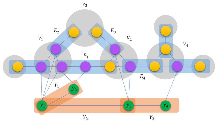
Figure 6: An $X$-web $\mathds{H}$, where $X$ consists of the vertices other than $y_{1},y_{2},y_{3},y_{4}$. Vertices $y_{1},\ldots,y_{4}$ are all $\mathds{H}$-tamed and ${\mathds{H}\hskip 1.19995pt}^{\dagger}$-tamed. $Y_{1}$ and $Y_{2}$ are $\mathds{H}$-wild and ${\mathds{H}\hskip 1.19995pt}^{\dagger}$-nonwild. $Y_{3}$ is $\mathds{H}$-wild and ${\mathds{H}\hskip 1.19995pt}^{\dagger}$-wild. $Y_{1}$ is $\mathds{H}$-solid. $Y_{2}$ and $Y_{3}$ are $\mathds{H}$-nonsolid. $E_{1}$, $E_{1}\cup E_{2}\cup E_{3}$, and $E_{1}\cup E_{2}\cup E_{3}\cup E_{4}$ are pods of $Y_{1}$ and $Y_{2}$ in $\mathds{H}$. $Y_{3}$ is $\mathds{H}$-unpodded. $Y_{1}$ and $Y_{2}$ are $\mathds{H}$-sticky and $Y_{3}$ is $\mathds{H}$-nonsticky.

3.1 Two major lemmas and our algorithm for detecting saplings

Let $\mathds{H}$ be an $X$-net. An $\mathds{H}$-wild set is a minimally $\mathds{H}$-untamed $Y\subseteq V(G-X)$ such that $G[Y]$ is a path. In Figure 6, $Y_{1}\cup Y_{2}$ is $\mathds{H}$-untamed but not $\mathds{H}$-wild, since $Y_{1}\subsetneq Y_{1}\cup Y_{2}$ is $\mathds{H}$-untamed. $\mathds{H}$ is not taming if and only if $G$ admits an $\mathds{H}$-wild set. An $S\subseteq X$ is $\mathds{H}$-solid if $S$ is a node of $\mathds{H}$ or $S$ is a subset of an arc $E=UV$ of $\mathds{H}$ such that $G[E]$ contains no $(S,U,V)$-sprout. If $S$ is a subset of a simple arc of $\mathds{H}$, then $S$ is $\mathds{H}$-solid if and only if $G[S]$ is an edge, since a sprout has to be an induced subgraph of $G$. Let $Y\subseteq V(G-X)$ such that $G[Y]$ is a path. $Y$ is $\mathds{H}$-solid if (1) $N(Y,X)$ is the union of two $\mathds{H}$-solid sets and (2) $N(y,X)=\varnothing$ for each internal vertex $y$, if any, of path $G[Y]$. A pod of $Y$ in $\mathds{H}$ is a $V_{1}V_{2}$-chunk $C$ of $\mathds{H}$ with the following Conditions P:

1. 1. $N(Y,X)\subseteq V_{1}\cup C\cup V_{2}$.

   2. For each $i\in\{1,2\}$, $N(y,V_{i})\subseteq C$ or $V_{i}\subseteq C\cup N(y)$ holds for an end-vertex $y$ of path $G[Y]$.

$Y$ is $\mathds{H}$-podded if $Y$ admits a pod in $\mathds{H}$. $Y$ is $\mathds{H}$-sticky if $Y$ is $\mathds{H}$-solid or $\mathds{H}$-podded. See Figure 6.

Lemma 3.2.

Let $Y$ be an ${\mathds{H}\hskip 1.19995pt}^{\dagger}$-wild set for an $X$-web $\mathds{H}$. (1) If $Y$ is $\mathds{H}$-nonsticky, then $G[X\cup Y]$ contains a sapling. (2) If $Y$ is $\mathds{H}$-sticky, then $\mathds{H}$ can be expanded to an $X\cup Y$-web.

By Lemmas 2.1 and 3.2 and Theorem 3.1, the following algorithm detects saplings in $G$:

Algorithm A

1. 1. If a sapling of $G$ is found (Lemma 2.1), then exit the algorithm.

   2. Let $X$-web $\mathds{H}$ be the obtained base net of $G$ and then repeat the following steps:

      1. If ${\mathds{H}\hskip 1.19995pt}^{\dagger}$ is taming, then report that $G$ is sapling-free (if-direction of Theorem 3.1) and exit.

      2. If ${\mathds{H}\hskip 1.19995pt}^{\dagger}$ is not taming, then obtain an ${\mathds{H}\hskip 1.19995pt}^{\dagger}$-wild set $Y$.

      3. If $Y$ is $\mathds{H}$-nonsticky, then report that $G[X\cup Y]$ contains a sapling (Lemma 3.2(1)) and exit.

      4. If $Y$ is $\mathds{H}$-sticky, then expand $\mathds{H}$ to an $X\cup Y$-web (Lemma 3.2(2)).

Lemma 3.3.

Algorithm A can be implemented to run in $O(m\log^{2}n)$ time.

3.2 Reducing Theorems 1.1, 2.2, and 3.1 to Lemmas 3.2 and 3.3 via aiding net

We need a relationship between simple paths in $\mathds{H}$ and induced paths in $G$. For any simple $UV$-path $\mathds{P}$ of $\mathds{H}$ (i.e., $U$ and $V$ are the end-nodes of $\mathds{P}$ in $\mathds{H}$), we define a $\mathds{P}$-rung of $G$ as a $UV$-rung of $G$ where all edges are contained in the arcs of $\mathds{P}$. Such a $\mathds{P}$-rung always exists by Conditions NN4 and NN6 of $\mathds{H}$ as long as $U\neq V$. For the degenerate case $U=V$, let $\mathds{P}$-rung be defined as the empty vertex set. For any distinct nodes $U_{1}$ and $U_{2}$ of $\mathds{H}$ intersecting a $V_{1}V_{2}$-chunk $C$ of $\mathds{H}$, there are disjoint $\mathds{U}\mathds{V}$-rungs $\mathds{P}_{1}$ and $\mathds{P}_{2}$ of $\mathds{H}$ with $\mathds{U}=\{U_{1},U_{2}\}$ and $\mathds{V}=\{V_{1},V_{2}\}$ by Condition NN1 of $\mathds{H}$. Since $\mathds{P}_{1}$ and $\mathds{P}_{2}$ are disjoint, any $\mathds{P}_{1}$-rung and $\mathds{P}_{2}$-rung of $G$ are disjoint and nonadjacent by Conditions NN2 and NN6 of $\mathds{H}$. Consider the $V_{1}V_{2}$-chunk $C=E_{1}\cup\cdots\cup E_{7}$ in Figure 4. Let $\mathds{V}=\{V_{1},V_{2}\}$. Let $\mathds{P}_{1}$ be the path of $\mathds{H}$ with arc $E_{3}$. Let $\mathds{P}_{2}$ be the path of $\mathds{H}$ with arc $E_{4}$. Let $\mathds{P}_{3}$ be the path of $\mathds{H}$ with arcs $E_{6}$ and $E_{7}$. Let $\mathds{P}_{4}$ be the degenerate path of $\mathds{H}$ consisting of a single node $V_{1}$. If $\mathds{U}=\{U_{1},U_{2}\}$, then $\mathds{P}_{1}$ and $\mathds{P}_{2}$ are disjoint $\mathds{U}\mathds{V}$-rungs. If $\mathds{U}=\{U_{1},W_{1}\}$, then $\mathds{P}_{1}$ and $\mathds{P}_{3}$ are disjoint $\mathds{U}\mathds{V}$-rungs of $\mathds{H}$. If $\mathds{U}=\{V_{1},W_{1}\}$, then $\mathds{P}_{3}$ and $\mathds{P}_{4}$ are disjoint $\mathds{U}\mathds{V}$-rungs of $\mathds{H}$. The path of $G$ induced by vertex set $\{11,12\}$ is the unique $\mathds{P}_{1}$-rung of $G$. The path of $G$ induced by vertex set $\{17,18\}$ is the unique $\mathds{P}_{2}$-rung of $G$. The paths induced by vertex sets $\{25,26,27,5,4,23\}$ and $\{25,26,28,7,6,24\}$ are the two $\mathds{P}_{3}$-rungs of $G$. The empty vertex set is the unique $\mathds{P}_{4}$-rung of $G$.

Lemma 3.4.

If $C$ is a $V_{1}V_{2}$-chunk of an $X$-net $\mathds{H}$, then applying $\textsc{merge}(C)$ on $\mathds{H}$ results in an $X$-net.

Proof.

Let ${\mathds{H}\hskip 0.80002pt}^{\prime}$ be the resulting $\mathds{H}$. Since any node cutset of ${\mathds{H}\hskip 0.80002pt}^{\prime}$ is also a node cutset of $\mathds{H}$, Conditions NN1 of ${\mathds{H}\hskip 0.80002pt}^{\prime}$ holds. Conditions NN2 and NN3 of ${\mathds{H}\hskip 0.80002pt}^{\prime}$ hold trivially. Conditions NN5 and NN6 of ${\mathds{H}\hskip 0.80002pt}^{\prime}$ follow from those of $\mathds{H}$. To see Condition NN4 of ${\mathds{H}\hskip 0.80002pt}^{\prime}$, let $x$ be a vertex in $C$. Let $E=U_{1}U_{2}$ be the arc of $\mathds{H}$ containing $x$. There are disjoint $\mathds{U}\mathds{V}$-rungs $\mathds{P}_{1}$ and $\mathds{P}_{2}$ of $\mathds{H}$ with $\mathds{U}=\{U_{1},U_{2}\}$ and $\mathds{V}=\{V_{1},V_{2}\}$. Let each $P_{i}$ with $i\in\{1,2\}$ be a $\mathds{P}_{i}$-rung of $G[C]$. Let $Q$ be a $U_{1}U_{2}$-rung of $G[E]$ containing $x$. $G[P_{1}\cup Q\cup P_{2}]$ is a $V_{1}V_{2}$-rung of $G[C]$ containing $x$. ∎

Lemma 3.5.

(1) If $G$ admits a taming net, then $G$ is sapling-free. (2) If an $X$-net $\mathds{H}$ has no parallel arcs, then every $\mathds{H}$-tamed subset of $X$ is $\mathds{H}$-local.

Since any $\mathds{H}$-local subset of $X$ for any $X$-net $\mathds{H}$ is $\mathds{H}$-tamed, Lemma 3.5(1) implies the if direction of Chudnovsky et al.’s Theorem 2.2. Moreover, by Lemma 3.5(2), the only-if direction of Theorem 3.1 implies the only-if direction of Theorem 2.2. Thus, our proofs for Lemma 3.5 and the only-if direction of Theorem 3.1 form a self-contained proof for Theorem 2.2.

Proof of Lemma 3.5.

Statement 1: Assume a taming net $\mathds{H}$ and a sapling $T$ of $G$ for contradiction. By Condition NN6 of $\mathds{H}$, any two adjacent vertices in $T$ contained by distinct arcs of $\mathds{H}$ belong to a node. If $G[Y]$ is a connected component of $T-X$, then vertices $u$ and $v$ of $T$ in $N(Y,X)$ belong to an arc of $\mathds{H}$: If $u$ and $v$ were in distinct arcs, then $\{u,v\}$ would be contained by a node of $\mathds{H}$, since $\mathds{H}$ is taming. By Condition NN6 of $\mathds{H}$, $uv$ is an edge of $G$, contradicting that $T$ is an induced tree. By Conditions NN2, NN3, and NN5 of $\mathds{H}$, the nodes and arcs of $\mathds{H}$ intersecting $T$ form a three-leaf connected subgraph $\mathds{T}$ of $\mathds{H}$. Thus, $T$ intersects a node of $\mathds{T}$ and three of its incident arcs in $\mathds{T}$. Condition NN6 implies a triangle in $T$, contradiction.

Statement 2: Assume an $\mathds{H}$-tamed $\mathds{H}$-nonlocal $S\subseteq X$ for contradiction. Let $E_{1},\ldots,E_{\ell}$ with $\ell\geq 2$ be the arcs of $\mathds{H}$ intersecting $S$. Since $S$ is $\mathds{H}$-tamed, any $E_{i}$ and $E_{j}$ with $1\leq i<j\leq\ell$ share a common end-node. If there is a common end-node $V$ of $E_{1},\ldots,E_{\ell}$, then the other end-nodes of $E_{i}$ with $i\in\{1,\ldots,\ell\}$ are pairwise distinct, since $\mathds{H}$ has no parallel arcs. Since $S$ is $\mathds{H}$-tamed, Condition NN6 implies $S\subseteq V$, contradicting that $S$ is $\mathds{H}$-nonlocal. Thus, $\ell=3$ and $E_{1},E_{2},E_{3}$ form a triangle of $\mathds{H}$. Since $S$ is $\mathds{H}$-nonlocal, there a vertex $x_{i}\in E_{i}\setminus V_{i}$ with $i\in\{1,2,3\}$ for an end-node $V_{i}$ of $E_{i}$. Let $x_{j}$ be a vertex of $S$ in the arc $E_{j}$ with $j\in\{1,2,3\}\setminus\{i\}$ incident to $V_{i}$. $\{x_{i},x_{j}\}\subseteq S$ is $\mathds{H}$-untamed, contradicting that $S$ is $\mathds{H}$-tamed. ∎

Proof of Theorems 1.1 and 3.1.

The if direction of Theorem 3.1 follows from Lemma 3.5(1). To see the only-if direction of Theorem 3.1, let $\mathds{H}$ be an $X$-web with maximum $|X|$ as ensured by Lemma 2.1. If ${\mathds{H}\hskip 1.19995pt}^{\dagger}$ were not taming, then any ${\mathds{H}\hskip 1.19995pt}^{\dagger}$-wild $Y$ would be $\mathds{H}$-sticky by Lemma 3.2(1), which in turn implies an $X\cup Y$-web by Lemma 3.2(2), contradicting the maximality of $\mathds{H}$. Thus Theorem 3.1 follows. By Lemmas 2.1 and 3.2 and the if direction of Theorem 3.1, Algorithm A correctly detects saplings in $G$. Thus, Theorem 1.1 follows from Lemma 3.3. ∎

Lemma 3.3 is not needed in the above reduction of Theorem 3.1 or else our proof of Theorem 2.2 would not be shorter than that in [28]. To complete proving Theorems 2.2 and 3.1, we prove Lemma 3.2 in §4. After that, to complete proving Theorem 1.1, we prove Lemma 3.3 in §5.

4 Proving Lemma 3.2

The following lemma is needed in the proofs of Lemma 3.2(1) in §4.1 and Lemma 3.2(2) in §4.2. For any chunk $C$ of a net $\mathds{H}$, the arc set $\mathds{C}$ of $\mathds{H}$ for $C$ consists of the arcs of $\mathds{H}$ that intersect $C$.

Lemma 4.1.

Let $\mathds{H}$ be an $X$-web. (1) If $Y$ is an ${\mathds{H}\hskip 1.19995pt}^{\dagger}$-wild set, then $Y$ is ${\mathds{H}\hskip 1.19995pt}^{\dagger}$-podded if and only if $Y$ is $\mathds{H}$-podded. (2) Each ${\mathds{H}\hskip 1.19995pt}^{\dagger}$-solid subset of $X$ is $\mathds{H}$-solid.

Proof.

Statement 1: The only-if direction is straightforward, since each $V_{1}V_{2}$-chunk of ${\mathds{H}\hskip 1.19995pt}^{\dagger}$ is a $V_{1}V_{2}$-chunk of $\mathds{H}$. For the if direction, let $C$ be a $V_{1}V_{2}$-chunk of $\mathds{H}$ that satisfies all Conditions P for $Y$. The maximal chunk of $\mathds{H}$ containing $C$ is an arc $E^{\dagger}=W_{1}W_{2}$ of ${\mathds{H}\hskip 1.19995pt}^{\dagger}$. By $N(Y,X)\subseteq V_{1}\cup C\cup V_{2}\subseteq W_{1}\cup E^{\dagger}\cup W_{2}$, Condition PP1 holds for $E^{\dagger}$ in ${\mathds{H}\hskip 1.19995pt}^{\dagger}$. Since $Y$ is ${\mathds{H}\hskip 1.19995pt}^{\dagger}$-untamed, $N(Y,X)$ intersects $(W_{1}\cup W_{2})\setminus E^{\dagger}$, implying $\{V_{1},V_{2}\}\cap\{W_{1},W_{2}\}\neq\varnothing$. Let $V_{1}=W_{1}$ and $W_{1}\setminus E^{\dagger}\subseteq V_{1}\setminus C\subseteq N(Y,X)$ without loss of generality. If $N(Y,X)$ does not intersect $W_{2}\setminus E^{\dagger}$, then Condition PP2 holds for $Y$ in ${\mathds{H}\hskip 1.19995pt}^{\dagger}$. Otherwise, we have $V_{2}=W_{2}$ and $W_{2}\setminus E^{\dagger}\subseteq V_{2}\setminus C\subseteq N(Y,X)$, also implying Condition PP2 of $Y$ in ${\mathds{H}\hskip 1.19995pt}^{\dagger}$. Thus, $E^{\dagger}$ is a pod of $Y$ in ${\mathds{H}\hskip 1.19995pt}^{\dagger}$.

Statement 2: It suffices to consider the case that the ${\mathds{H}\hskip 1.19995pt}^{\dagger}$-solid subset $S$ of $X$ is not a node of $\mathds{H}$, implying that $S$ is not a node of ${\mathds{H}\hskip 1.19995pt}^{\dagger}$. Let $\mathds{W}=\{W_{1},W_{2}\}$ for the arc $C=W_{1}W_{2}$ of ${\mathds{H}\hskip 1.19995pt}^{\dagger}$ with $S\subseteq C$. $G[C]$ contains no $(S,W_{1},W_{2})$-sprout. The rest of the proof lets all sprouts be $(S,W_{1},W_{2})$-sprouts unless explicitly specified otherwise. Let $E_{i}$ with $1\leq i\leq|\mathds{C}|$ be the arcs in the arc set $\mathds{C}$ of $\mathds{H}$ for $C$. Let $\mathds{V}_{i}$ consist of the end-nodes of $E_{i}$. For any $i$ and $j$ that may not be distinct, let $\mathds{P}_{i,j}$ and $\mathds{Q}_{i,j}$ be disjoint $\mathds{W}\mathds{V}_{i}$-rung and $\mathds{W}\mathds{V}_{j}$-rung of $\mathds{H}$. Let $P_{i,j}$ be a $\mathds{P}_{i,j}$-rung of $G$. Let $Q_{i,j}$ be a $\mathds{Q}_{i,j}$-rung of $G$. Let $U_{i,j}$ be the end-node of $\mathds{P}_{i,j}$ in $\mathds{V}_{i}$. Let $V_{i,j}$ be the end-node of $\mathds{Q}_{i,j}$ in $\mathds{V}_{j}$. If $S\subseteq E_{i}$ for an $i\in\{1,\ldots,|\mathds{C}|\}$, then $G[E_{i}]$ contains no $(S,U_{i,i},V_{i,i})$-sprout $T$ or else $G[T\cup P_{i,i}\cup Q_{i,i}]$ would be a sprout of $G[C]$. Thus, $S$ is $\mathds{H}$-solid. The rest of the proof assumes for contradiction that $S$ intersects two or more arcs of $\mathds{C}$.

We first show that $S$ is contained by a node of $\mathds{H}$. For any distinct $i$ and $j$ such that $S$ intersects both $E_{i}$ and $E_{j}$, let $r$ be an arbitrary vertex in $S\cap E_{i}$ and $s$ be an arbitrary vertex in $S\cap E_{j}$. Let $P=G[P_{i,j}\cup P^{\prime}]$ and $Q=G[Q_{i,j}\cup Q^{\prime}]$ for arbitrary $rU_{i,j}$-rung $P^{\prime}$ of $G[E_{i}]$ and $sV_{i,j}$-rung $Q^{\prime}$ of $G[E_{j}]$. By Conditions NN2 and NN5, $P-r$ and $Q-s$ are disjoint and nonadjacent, implying that $r$ and $s$ are adjacent or else $G[P\cup Q]$ would contain a sprout of Type SS2 in $G[C]$. Since $r$ and $s$ are arbitrary, Condition NN6 implies $S\subsetneq U$ for a node $U$ of $\mathds{H}$: If $S$ is not contained by any node of $\mathds{H}$, then $S$ is contained by $\Delta(V_{1},V_{2},V_{3})$ and intersects $V_{1}\cup V_{2}$, $V_{2}\cap V_{3}$, and $V_{3}\cap V_{1}$ for nodes $V_{1},V_{2},V_{3}$ of $\mathds{H}$. Let $\mathds{V}=\{V_{1},V_{2},V_{3}\}$. Let $\mathds{P}_{i}$ and $\mathds{P}_{j}$ with $\{i,j\}\subseteq\{1,2,3\}$ be disjoint $\mathds{V}\mathds{W}$-rungs of $\mathds{C}$ such that $V_{i}$ and $V_{j}$ are the end-nodes of $\mathds{P}_{i}$ and $\mathds{P}_{j}$ in $\mathds{V}$. $G[P_{i}\cup\{v\}\cup P_{j}]$ for $v\in S\cap V_{i}\cap V_{j}$ and $\mathds{P}_{i}$-rung $P_{i}$ and $\mathds{P}_{j}$-rung $P_{j}$ of $G[C]$ is a sprout of Type SS1, contradiction.

For any arcs $E_{i}=UV_{i}$ and $E_{j}=UV_{j}$ of $\mathds{C}$ with $V_{i}\neq V_{j}$, we say that $E_{i}$ evades $E_{j}$ if there are disjoint $\mathds{V}\mathds{W}$-rungs $\mathds{P}$ and $\mathds{Q}$ of $\mathds{H}$ with $\mathds{V}=\{V_{i},V_{j}\}$ such that $\mathds{P}\cup\mathds{Q}$ does not intersect $U$. $E_{i}$ evades $E_{j}$ if and only if $E_{j}$ evades $E_{i}$. If $E_{i}$ evades $E_{j}$ and $E_{i}$ intersects $S$, then $E_{j}\cap U\subseteq S$ or else $G[C]$ would contain a sprout $G[P_{i}\cup Q_{j}\cup P\cup Q]$ of Type SS1, where $P_{i}$ is an $E_{i}$-rung intersecting $S$, $Q_{j}$ is an $E_{j}$-rung intersecting $U\setminus S$, $P$ is a $\mathds{P}$-rung, and $Q$ is a $\mathds{Q}$-rung.

By $S\subsetneq U$, $E_{j}\cap U\not\subseteq S$ holds for an arc $E_{j}=UV_{j}$. If each arc $E_{i}=UV_{i}$ intersecting $S$ satisfies $V_{i}=V_{j}$, then $G[P_{i,i}\cup Q_{i,i}\cup R]$ for any $UV_{i}$-rung $R$ of $G[E_{i}]$ that intersects $S$ is a sprout of Type SS1, contradiction. Thus, an arc $E_{i}=UV_{i}$ with $V_{i}\neq V_{j}$ intersects $S$. By $E_{j}\cap U\nsubseteq S$ and $E_{i}\cap S\neq\varnothing$, $E_{i}$ does not evade $E_{j}$. We show contradiction by identifying an arc $E_{k}=UV_{k}$ with $V_{k}\notin\{V_{i},V_{j}\}$ such that $E_{i}$ evades $E_{k}$, implying $E_{k}\cap U\subseteq S$, and $E_{k}$ evades $E_{j}$, implying $E_{k}\cap S=\varnothing$. Let $\mathds{P}_{i}$ and $\mathds{P}_{j}$ be disjoint $\mathds{V}\mathds{W}$-rungs of $\mathds{H}$ with $\mathds{V}=\{V_{i},V_{j}\}$. Since $E_{i}$ does not evade $E_{j}$, $\mathds{P}_{i}\cup\mathds{P}_{j}$ intersects $U$. Let $\mathds{P}_{j}$ intersect $U$ without loss of generality. $U$ is the neighbor of $V_{j}$ in $\mathds{P}_{j}$. Let $E_{k}=UV_{k}$ be the incident arc of $U$ in $\mathds{P}_{j}$ with $V_{k}\neq V_{j}$. Let $\mathds{Q}=\mathds{P}_{j}-\{U,V_{j}\}$. Since $\mathds{P}_{i}$ and $\mathds{Q}$ are disjoint $\mathds{V}\mathds{W}$-rungs of $\mathds{H}$ with $\mathds{V}=\{V_{i},V_{k}\}$ and $\mathds{P}_{i}\cup\mathds{Q}$ does not intersect $U$, $E_{i}$ evades $E_{k}$. Let $\mathds{R}^{\prime}$ be a rung of $(\mathds{C}\cup\{W_{1}W_{2}\})-U$ between $V_{j}$ and $\mathds{P}_{i}$. $\mathds{R}^{\prime}$ does not intersect $\mathds{Q}$ or else $E_{i}$ would evade $E_{j}$. Let $\mathds{R}$ be the $V_{j}\mathds{W}$-rung of $\mathds{P}_{i}\cup\mathds{R}^{\prime}$. Since $\mathds{Q}$ and $\mathds{R}$ are disjoint $\mathds{V}\mathds{W}$-rungs of $\mathds{H}$ with $\mathds{V}=\{V_{k},V_{j}\}$ and $\mathds{Q}\cup\mathds{R}$ does not intersect $U$, $E_{k}$ evades $E_{j}$. ∎

4.1 Proving Lemma 3.2(1)

A net self-aids if it aids itself. Since the aiding net of any web self-aids, Lemma 3.2(1) is immediate from Lemma 4.2 by Lemma 4.1.

Lemma 4.2.

For self-aiding $X$-net $\mathds{H}_{0}$ and $\mathds{H}_{0}$-wild $\mathds{H}_{0}$-nonsticky set $Y$, $G[X\cup Y]$ contains a sapling.

The rest of the subsection proves Lemma 4.2 using Lemmas 4.3, 4.4, and 4.5. Let $\mathds{L}$ consist of the leaves of the self-aiding net $\mathds{H}$ in Lemma 4.3, 4.4, or 4.5. Since $\nabla(\mathds{H})$ is triconnected, each nonleaf node of $\mathds{H}$ has degree at least three in $\mathds{H}$ and any three-node set $\mathds{U}$ of $\mathds{H}$ admits pairwise disjoint $\mathds{U}\mathds{L}$-rungs $\mathds{P}_{1},\mathds{P}_{2},\mathds{P}_{3}$ of $\mathds{H}$. By Condition NN6 of $\mathds{H}$, any $\mathds{P}_{i}$-rungs $P_{i}$ of $G$ with $i\in\{1,2,3\}$ are pairwise disjoint and nonadjacent.

Lemma 4.3.

If $Y$ is an $\mathds{H}$-wild $\mathds{H}$-nonsticky set for a self-aiding $X$-net $\mathds{H}$ of $G$ such that $N_{G}(Y,X)=M_{1}\cup M_{2}$ and each of $M_{1}$ and $M_{2}$ is contained by a node or arc of $\mathds{H}$, then $G[X\cup Y]$ contains a sapling.

Proof.

Let $N=N_{G}(Y,X)$. We start with proving the following statement.

Claim 1: If $M_{i}\subseteq U$ with $\{i,j\}=\{1,2\}$ holds for a node $U$ and $M_{j}\subseteq U_{1}\cup F$ holds for an end-node $U_{1}$ of an arc $F$ with $U_{1}\neq U$, $U\setminus F\nsubseteq M_{i}$, and $M_{i}\nsubseteq F$, then $G[X\cup Y]$ contains a sapling.

Let $\mathds{R}_{1}=\{U_{1}\}$. Since the degree of $U$ is at least three, $U\setminus F\nsubseteq M_{i}$ and $M_{i}\nsubseteq F$ imply that the node set consisting of the neighbors of $U$ other than $U_{1}$ in $\mathds{H}$ admits a nonempty disjoint partition $\mathds{R}_{2}$ and $\mathds{R}_{3}$ such that (a) each arc between $U$ and $\mathds{R}_{2}$ intersects $M_{i}$ and (b) each arc between $U$ and $\mathds{R}_{3}$ intersects $U\setminus M_{i}$. Let ${\mathds{H}\hskip 0.80002pt}^{\prime}$ be the triconnected graph obtained from $\nabla(\mathds{H})$ by (1) replacing node $U$ and its incident arcs with a triangle on a set $\mathds{W}=\{W_{1},W_{2},W_{3}\}$ of three new nodes and (2) adding an arc between $W_{i}$ and each node in $\mathds{R}_{i}$ for all $i\in\{1,2,3\}$. There are pairwise disjoint $\mathds{W}\mathds{L}$-rungs $\mathds{P}_{1},\mathds{P}_{2},\mathds{P}_{3}$ of ${\mathds{H}\hskip 0.80002pt}^{\prime}$ such that each $\mathds{P}_{i}$ with $i\in\{1,2,3\}$ is a $W_{i}L_{i}$-rung with $L_{i}\in\mathds{L}$. Let $\mathds{Q}_{1}$ be the path of $\mathds{H}$ consisting of arc $F$ and path $\mathds{P}_{1}-W_{1}$. Let $Q_{1}$ be the $NL_{1}$-rung of a $\mathds{Q}_{1}$-rung of $G$ intersecting $M_{j}$. Let $\mathds{Q}_{2}$ be the $L_{2}L_{3}$-path of $\mathds{H}$ obtained from $\mathds{P}_{2}\cup\mathds{P}_{3}$ by replacing the two arcs $W_{2}U_{2}$ and $W_{3}U_{3}$ with the two arcs $UU_{2}$ and $UU_{3}$. Let $Q_{2}$ be a $\mathds{Q}_{2}$-rung of $G$ intersecting exactly one vertex in $M_{i}\cap U$. $N$ intersects each of $Q_{1}$ and $Q_{2}$ at exactly one vertex. Thus, $G[Y\cup Q_{1}\cup Q_{2}]$ contains a sapling of $G[X\cup Y]$. Claim 1 is proved.

Claim 2: If $G[X\cup Y]$ is sapling-free, then each $M_{i}$ with $i\in\{1,2\}$ is $\mathds{H}$-solid.

To prove Claim 2 by Claim 1, let each $M_{i}$ with $i\in\{1,2\}$ be contained by a node $V_{i}$ or an arc $E_{i}$. We first show that if $M_{1}\subseteq V_{1}$ and $M_{2}\subseteq V_{2}$, then $V_{1}V_{2}$ is not an arc. Assume an arc $E=V_{1}V_{2}$ for contradiction. Since $Y$ is $\mathds{H}$-wild and $\mathds{H}$-unpodded, we have $V_{i}\nsubseteq(E\cup M_{i})$ and $M_{i}\nsubseteq E$ for $\{i,j\}=\{1,2\}$, contradicting Claim 1 with $U=V_{i}$, $U_{1}=V_{j}$, and $F=E$.

To see Claim 2(a): $M_{i}\subseteq V_{i}$ for $\{i,j\}=\{1,2\}$ implies $M_{i}=V_{i}$, assume $V_{i}\nsubseteq M_{i}$. If $M_{j}\subseteq V_{j}$, then $V_{i}V_{j}$ is not an arc, contradicting Claim 1 with $U=V_{i}$, $U_{1}=V_{j}$, and $F$ being an incident arc of $V_{j}$. $M_{j}\subseteq E_{j}$ contradicts Claim 1 with $U=V_{i}$, $F=E_{j}$, and $U_{1}$ being an end-node of $E_{j}$ that is not $V_{i}$. To see Claim 2(b): $M_{i}\subseteq E_{i}=UV$ for $\{i,j\}=\{1,2\}$ implies that $M_{i}$ is $\mathds{H}$-solid, assume an $(M_{i},U,V)$-sprout $T$ of $G[E_{i}]$. If $M_{j}\subseteq V_{j}$, then let $W=V_{j}$. By Claim 2(a), $W$ is not incident to $E_{i}$ or else $E_{i}$ would be a pod of $Y$ in $\mathds{H}$. If $M_{j}\subseteq E_{j}$, then let $W$ be an end-node of $E_{j}$ not incident to $E_{i}$. Let $\mathds{U}=\{U,V,W\}$. Let $\mathds{P}_{1},\mathds{P}_{2},\mathds{P}_{3}$ be pairwise disjoint $\mathds{U}\mathds{L}$-rungs of $\mathds{H}$. Let each $P_{k}$ with $k\in\{1,2,3\}$ be a $\mathds{P}_{k}$-rung of $G$. $G[P_{1}\cup P_{2}\cup P_{3}\cup Y\cup T\cup E_{j}]$ contains a sapling.

To prove the lemma by Claim 2, assume for contradiction that $G[X\cup Y]$ is sapling-free. Since $Y$ is $\mathds{H}$-nonsolid, Claim 2 implies an internal vertex $y$ of path $G[Y]$ with nonempty $N_{G}(y,X)\subseteq M_{1}\cap M_{2}$. By Condition NN2, $M_{i}=V_{i}$ holds for $\{i,j\}=\{1,2\}$. By Condition NN5, if $M_{j}\subseteq V_{j}$, then $\mathds{H}$ has an arc $E=V_{i}V_{j}$, which is a pod of $Y$ in $\mathds{H}$; and if $M_{j}\subseteq E_{j}$, then $V_{i}$ is incident to $E_{j}$, which is thus a pod of $Y$ in $\mathds{H}$. Both cases contradict that $Y$ is $\mathds{H}$-nonsticky. ∎

If $Y$ is $\mathds{H}$-wild for an $X$-net $\mathds{H}$, then let $\ell(Y,\mathds{H},G)$ denote the minimum number of $\mathds{H}$-tamed subsets of $X$ whose union is $N_{G}(Y,X)$. A net is simple if all of its arcs are simple. If $\mathds{H}$ is a simple self-aiding $X$-net of $G$, then $G[X]$ is isomorphic to the line graph of a subdivision of $\mathds{H}$.

Lemma 4.4.

If $Y$ is an $\mathds{H}$-wild set for a simple self-aiding $X$-net $\mathds{H}$ of $G$ with $\ell(Y,\mathds{H},G)=2$ such that $N_{G}(Y,X)$ contains a triad of $\mathds{H}$, then $G[X\cup Y]$ contains a sapling.

Proof.

Let $\mathds{U}=\{U_{1},U_{2},U_{3}\}$ for nodes with $\Delta=\Delta(U_{1},U_{2},U_{3})\subseteq N=N_{G}(Y,X)$. Let $\mathds{P}_{1},\mathds{P}_{2},\mathds{P}_{3}$ be pairwise disjoint $\mathds{U}\mathds{L}$-rungs of $\mathds{H}$. For each $i\in\{1,2,3\}$, let $L_{i}\in\mathds{L}$ such that the $\mathds{P}_{i}$-rung $P_{i}$ of $G$ is a $U_{i}L_{i}$-rung. Since $N$ is untamed, $N\setminus\Delta\neq\varnothing$. Since $\mathds{H}$ is simple, each arc intersecting $N\setminus\Delta$ is incident to at most one node of $\mathds{U}$. By $\ell(Y,\mathds{H},G)=2$, $N\setminus\Delta$ intersects at most one of $P_{1}$, $P_{2}$, and $P_{3}$. If $N$ intersects $P_{i}$ for $\{i,j,k\}=\{1,2,3\}$, then $G[Y\cup Q_{i}\cup(U_{j}\cap U_{k})\cup P_{j}\cup P_{k}]$ contains a sapling for the $NL_{i}$-rung $Q_{i}$ of $P_{i}$. It remains to consider $(N\setminus\Delta)\cap V(P_{1}\cup P_{2}\cup P_{3})=\varnothing$.

Case 1: Each arc $E$ intersecting $N\setminus\Delta$ satisfies $|E|=1$ and is incident to $\mathds{P}_{i}$ and $\mathds{P}_{j}$ for $\{i,j,k\}=\{1,2,3\}$. Let $E$ be an arc intersecting $N\setminus\Delta$. Let $V_{i}\in V(\mathds{P}_{i})$ and $V_{j}\in V(\mathds{P}_{j})$ be end-nodes of $E$ with $U_{i}\neq V_{i}$. Let $\mathds{Q}_{1}$ be the $U_{i}L_{k}$-path of $\mathds{H}$ consisting of arc $E_{j}=U_{i}U_{k}$ and $\mathds{P}_{k}$. Let $Q_{1}$ be the $\mathds{Q}_{1}$-rung of $G$. Let $\mathds{Q}_{2}$ be the $L_{i}L_{j}$-path of $\mathds{H}$ consisting of $E$, the $V_{i}L_{i}$-rung of $\mathds{P}_{i}$, and the $V_{j}L_{j}$-rung of $\mathds{P}_{j}$. Let $Q_{2}$ be the $\mathds{Q}_{2}$-rung of $G$. By $U_{i}\neq V_{i}$, $\mathds{Q}_{1}$ and $\mathds{Q}_{2}$ are disjoint. By $(N\setminus\Delta)\cap V(P_{1}\cup P_{2}\cup P_{3})=\varnothing$, $Q_{1}$ (respectively, $Q_{2}$) intersects $N$ exactly at the vertex in arc $E_{j}$ (respectively, $E$). Thus, $G[Y\cup Q_{1}\cup Q_{2}]$ contains a sapling of $G[X\cup Y]$.

Case 2: An arc $E$ intersecting $N\setminus\Delta$ violates the condition of Case 1. Let $\mathds{Q}$ be a shortest path of $\mathds{H}$ between $V(E)$ and $V(\mathds{P}_{1}\cup\mathds{P}_{2}\cup\mathds{P}_{3})$. Since $E$ violates the condition of Case 1, we may require that if $U\in V(E)$ and $V_{i}\in V(\mathds{P}_{i})$ with $\{i,j,k\}=\{1,2,3\}$ are the end-nodes of $\mathds{Q}$, then the $NU$-rung $Q_{i}$ of $G[E]$ is not adjacent to $P_{j}\cup P_{k}$. Let $E_{i}=U_{j}U_{k}$. Let $Q$ be the $\mathds{Q}$-rung of $G$. Let $R_{i}$ be the $V_{i}L_{i}$-rung of $P_{i}$. $G[P_{j}\cup P_{k}\cup E_{i}\cup Q_{i}\cup Q\cup R_{i}]$ contains a sapling of $G[X\cup Y]$. ∎

Lemma 4.5.

Let $Y$ be an $\mathds{H}$-wild set for a simple self-aiding $X$-net $\mathds{H}$ of graph $G$ with $\ell(Y,\mathds{H},G)\geq 3$. If $G[X\cup Y]$ is sapling-free, then $Y$ is $\mathds{H}$-podded for $G$.

Proof.

Since $Y$ is $\mathds{H}$-wild with $\ell=\ell(Y,\mathds{H},G)\geq 3$, $Y$ consists of a vertex $y$. Let $N_{1},\ldots,N_{\ell}$ be pairwise disjoint $\mathds{H}$-tamed subsets of $X$ whose union is $N=N_{G}(Y,X)$. Let $L$ consist of the leaves of $H=G[X\cup Y]$. Let each graph $H_{i,j}$ with $1\leq i<j\leq\ell$ be obtained from $H$ by deleting the edges between $y$ and $N\setminus(N_{i}\cup N_{j})$. We claim that each $H_{i,j}$ is sapling-free. Since $\mathds{H}$ is a simple self-aiding $X$-net of $H_{i,j}$ with $\ell(Y,\mathds{H},H_{i,j})=2$, $Y$ is $\mathds{H}$-sticky for $H_{i,j}$ by Lemmas 4.3 and 4.4. Thus, each $N_{i}$ with $i\in\{1,\ldots,\ell\}$ is either contained by a node or arc of $\mathds{H}$. Assume that $N_{1},\ldots,N_{k}$ are $\mathds{H}$-solid and $N_{k+1},\ldots,N_{\ell}$ are not. If $k<\ell$, then $Y$ is $\mathds{H}$-podded for all $H_{i,\ell}$ with $i\in\{1,\ldots,\ell-1\}$. If $N_{\ell}$ is contained by a node $U$, then there is exactly one vertex $u$ in $U\setminus N_{\ell}$, implying $\ell=3$ and that the arc containing $u$ is a pod of $Y$ in $\mathds{H}$ for $G$. If $N_{\ell}$ is not contained by a node, then $\ell=3$ and the arc containing $N_{\ell}$ is a pod of $Y$ in $\mathds{H}$ for $G$. As for $k=\ell$, observe that there cannot be a $3$-node set $\mathds{U}=\{U_{i_{1}},U_{i_{2}},U_{i_{3}}\}$ with $\{i_{1},i_{2},i_{3}\}\subseteq\{1,\ldots,\ell\}$ such that each node $U_{i_{j}}$ with $j\in\{1,2,3\}$ is either a solid set $N_{i_{j}}$ or an end-node of the arc $E_{i_{j}}$ containing a solid set $N_{i_{j}}$: Assume for contradiction that such a $\mathds{U}$ exists. Let vertex set $E$ be the union of the arcs $E_{i_{j}}$ with $N_{i_{j}}\subseteq E_{i_{j}}$. Let $\mathds{P}_{1}$, $\mathds{P}_{2}$, and $\mathds{P}_{3}$ be pairwise disjoint $\mathds{U}\mathds{L}$-rungs of $\mathds{H}$. For each $j\in\{1,2,3\}$, let $P_{j}$ be a $\mathds{P}_{j}$-rung of $G$. $G[Y\cup P_{1}\cup P_{2}\cup P_{3}\cup E]$ contains a sapling, contradiction. The observation implies $\ell=3$ and that $Y$ is $\mathds{H}$-podded for $G$.

To prove the claim, assume a sapling $T$ of $H_{i,j}$. Since any edge in $H[T]\setminus T$ is between $y$ and $N_{i,j}$, the following statements hold or else $H$ would contain a sapling in which $y$ is the degree-$3$ vertex: (1) The degree of $y$ in $T$ is two. (2) $H[T]\setminus T$ has exactly one edge $e$, implying that $y$ and a vertex $u_{1}\in N_{i,j}$ are the end-vertices of $e$. (3) The degree-$3$ vertex $u_{2}$ of $T$ is adjacent to $y$ and $u_{1}$ in $T$, implying $u_{2}\in N_{i}\cup N_{j}$. That is, $H[T]$ consists of a triangle on $U=\{y,u_{1},u_{2}\}$ and pairwise disjoint $UL$-rungs $P_{1},P_{2},P_{3}$ of $T$ with $N\cap V(P_{1})=\{u_{1}\}\subseteq N_{i_{1}}$, $N\cap V(P_{2})=\{u_{2}\}\subseteq N_{i_{2}}$, and $y\in V(P_{3})$ for distinct $i_{1}$ and $i_{2}$ in $\{1,\ldots,\ell\}$. By Lemma 3.5(2), each $N_{i_{k}}$ with $k\in\{1,2\}$ is contained by a node, arc, or triad $S_{k}$. $N\cap(S_{1}\cup S_{2})$ is $\mathds{H}$-untamed or else there would be $\ell-1$ pairwise disjoint $\mathds{H}$-tamed subsets of $X$ whose union is $N$. Let each $E_{k}$ with $k\in\{1,2\}$ be the simple arc with $u_{k}\in E_{k}$. We show that $H$ contains a sapling in which $y$ is the degree-$3$ vertex.

Case 1: If $E_{1}=E_{2}$. Since $N\cap(S_{1}\cup S_{2})$ is $\mathds{H}$-untamed, a vertex $v_{k}\in S_{k}\cap(N\setminus E_{k})$ with $k\in\{1,2\}$. Since $\mathds{H}$ is simple and $\{u_{k},v_{k}\}\subseteq S_{k}$, $S_{k}$ is not a triad. $S_{k}$ is not an arc or else $E_{k}=S_{k}$ would intersect $N\setminus E_{k}$. Thus, $S_{k}$ is an end-node of $E_{k}$ with $\{u_{k},v_{k}\}\subseteq S_{k}$ and $u_{3-k}\notin S_{k}$. By $u_{k}\in S_{k}$ and Condition NN6, $S_{k}$ is not adjacent to $(P_{3}-y)\cup(P_{3-k}-u_{3-k})$ in $H$. Since $\mathds{H}$ is simple, $v_{k}\in N\cap S_{k}$ implies that $H[(T-u_{k})\cup\{v_{k}\}]$ is a sapling of $H$.

Case 2: $E_{1}\neq E_{2}$. By Condition NN5, $\{u_{1},u_{2}\}\subseteq V$ for a common end-node $V$ of arcs $E_{1}$ and $E_{2}$. By Condition NN6, $E_{k}\subseteq V(P_{k})$ for each $k\in\{1,2\}$. Since $N\cap(S_{1}\cup S_{2})$ is $\mathds{H}$-untamed, a vertex $v_{k}\in S_{k}\cap(N\setminus V)$ with $k\in\{1,2\}$. Since $\mathds{H}$ is simple and $\{u_{k},v_{k}\}\subseteq S_{k}$, $S_{k}$ is not a triad. $S_{k}$ is not an arc or else $\{u_{k},v_{k}\}\subseteq S_{k}=E_{k}\subseteq V(P_{k})$ would contradict $N\cap V(P_{k})=\{u_{k}\}$. Thus, $S_{k}$ is a node. By $u_{k}\in E_{k}\cap S_{k}$, $S_{k}$ is an end-node of $E_{k}$ containing $u_{k}$. By $v_{k}\in S_{k}\setminus V$, $S_{k}\neq V$. By $u_{k}\in S_{k}$ and Condition NN6, $S_{k}$ is not adjacent to $V(P_{3}-y)\cup V(P_{3-k}-u_{3-k})$ in $H$. Since $\mathds{H}$ is simple, $v_{k}\in N\cap S_{k}$ implies that $H[(T-u_{k})\cup\{v_{k}\}]$ is a sapling of $H$. ∎

Proof of Lemma 4.2.

Assume for contradiction that $G[X\cup Y]$ is sapling-free. A vertex set $D\subseteq X$ is an inducing set of $\mathds{H}_{0}$ if $G[E_{0}\cap D]$ for each arc $E_{0}=U_{0}V_{0}$ is an $U_{0}V_{0}$-rung of $G[E_{0}]$. For any inducing set $D$ of $\mathds{H}_{0}$, let $\mathds{H}_{0}(D)$ denote the simple self-aiding $D$-net of graph $H_{0}(D)=G[Y\cup D]$ obtained from $\mathds{H}_{0}$ by replacing each arc $E_{0}$ of $\mathds{H}_{0}$ with the arc $E=E_{0}\cap D$ and replacing each node $V_{0}$ of $\mathds{H}_{0}$ with the node $V=V_{0}\cap D$. Let $N=N_{G}(Y,X)$. Let $\ell=\ell(Y,\mathds{H}_{0},G)$. If $\ell=2$, then Lemma 4.3 implies $N\nsubseteq S_{1}\cup S_{2}$ for any node or arc $S_{i}$ of $\mathds{H}_{0}$ with $i\in\{1,2\}$. Thus, $N$ contains a triad $\Delta$ and $N\setminus\Delta$ is not contained by any arc of $\mathds{H}_{0}$ between two nodes of $\Delta$. By $\ell=2$, there is an inducing set $D$ of $\mathds{H}_{0}$ with $\ell(Y,\mathds{H}_{0}(D),H_{0}(D))=2$ and $\Delta\subseteq N_{H_{0}(D)}(Y,D)$, contradicting Lemma 4.4. Thus, $\ell\geq 3$, implying a three-vertex set $S\subseteq N$ such that every two-vertex subset of $S$ is $\mathds{H}_{0}$-untamed. Let $D$ be an inducing set of $\mathds{H}_{0}$ with $S\subseteq D$, implying $\ell(Y,\mathds{H}_{0}(D),H_{0}(D))\geq 3$. By Lemma 4.5, there is a pod $E=UV$ of $Y$ in $\mathds{H}_{0}(D)$ for $H_{0}(D)$ such that $N_{H_{0}(D)}(Y)$ intersects $E\setminus(U\cup V)$, $U\setminus E$, and $V\setminus E$. Let $E_{0}=U_{0}V_{0}$ be the arc of $\mathds{H}_{0}$ with $E=E_{0}\cap D$, $U=U_{0}\cap D$, and $V=V_{0}\cap D$. Since $E_{0}$ is not a pod of $Y$ in $\mathds{H}_{0}$ and $N$ intersects $E_{0}\setminus(U_{0}\cup V_{0})$, $U_{0}\setminus E_{0}$, and $V_{0}\setminus E_{0}$, a vertex $x$ belongs to $N\setminus(U_{0}\cup E_{0}\cup V_{0})$ or $(U_{0}\cup V_{0})\setminus(E_{0}\cup N)$. Let $D^{\prime}$ be an inducing set $(D\setminus E_{0})\cup V(P)$ of $\mathds{H}_{0}$, where $E_{0}=U_{0}V_{0}$ is the arc of $\mathds{H}_{0}$ containing $x$ and $P$ is a $U_{0}V_{0}$-rung of $G[E_{0}]$ containing $x$. One can verify that $Y$ is $\mathds{H}_{0}(D^{\prime})$-unpodded for $H_{0}(D^{\prime})$ with $\ell(Y,\mathds{H}_{0}(D^{\prime}),H_{0}(D^{\prime}))\geq 3$, contradicting Lemma 4.5. ∎

4.2 Proving Lemma 3.2(2)

This subsection shows that if $Y$ is $\mathds{H}$-sticky for an $X$-web $\mathds{H}$, then $\mathds{H}$ can be expanded to an $X\cup Y$-web via Subroutine B below. Let $\mathds{H}$ be an $X$-net. For any $\mathds{H}$-solid subset $S$ of $X$ contained by a simple arc $F=U_{1}U_{2}$ of $\mathds{H}$, define Operation $\textsc{subdivide}(S)$ to (1) create a new node $S$ and (2) replace the simple arc by new simple arcs $SU_{i}$ with $i\in\{1,2\}$ consisting of the vertices of the $SU_{i}$-rung of $G[F]$. Define Subroutine B with $N=N(Y,X)$ as follows (see Figure 7):

Subroutine B

1. 1. $Y$ is $\mathds{H}$-solid. Let $S_{1}$ and $S_{2}$ be $\mathds{H}$-solid sets with $N=S_{1}\cup S_{2}$.

      1. For each $i\in\{1,2\}$, if $S_{i}$ is contained by a simple arc, then create node $S_{i}$ by $\textsc{subdivide}(S_{i})$.

      2. Add each end-vertex $y$ of path $G[Y]$ into the nodes $S_{i}$ with $i\in\{1,2\}$ and $S_{i}\subseteq N(y)$.

      3. Make a simple arc $Y=S_{1}S_{2}$.

   2. $Y$ is $\mathds{H}$-nonsolid. Thus, $Y$ is $\mathds{H}$-podded. Let $V_{1}V_{2}$-chunk $C$ of $\mathds{H}$ be a minimal pod of $Y$ in $\mathds{H}$. Since $Y$ is ${\mathds{H}\hskip 1.19995pt}^{\dagger}$-wild, assume $V_{1}\in V({\mathds{H}\hskip 1.19995pt}^{\dagger})$ and $V_{1}\subseteq C\cup N$ without loss of generality.

      1. If $V_{2}$ is incident to exactly one arc $F=VV_{2}$ in the arc set for $C$, $N\cap V_{2}\subseteq F$, and $F$ is simple, then $N$ intersects $F\setminus V$ by the minimality of $C$. Let $v_{2}$ be the end-vertex of the $NV_{2}$-rung $P$ of $G[F]$ in $N$. Let $v$ be the neighbor of $v_{2}$ not in $P$. Call $\textsc{subdivide}(\{v,v_{2}\})$ to create a new node $V_{2}=\{v,v_{2}\}$. Delete $V(P)$ from $C$ to preserve that $C$ is a $V_{1}V_{2}$-chunk that is a minimal pod of $Y$ in $\mathds{H}$.

      2. Update $\mathds{H}$ by $\textsc{merge}(C)$. Let $E=V_{1}V_{2}$ be the arc of $\mathds{H}$ with $E=C$.

      3. Add $Y$ to arc $E$ and add each end-vertex $y$ of path $G[Y]$ to the nodes $V_{i}$ with $V_{i}\subseteq C\cup N(y)$.

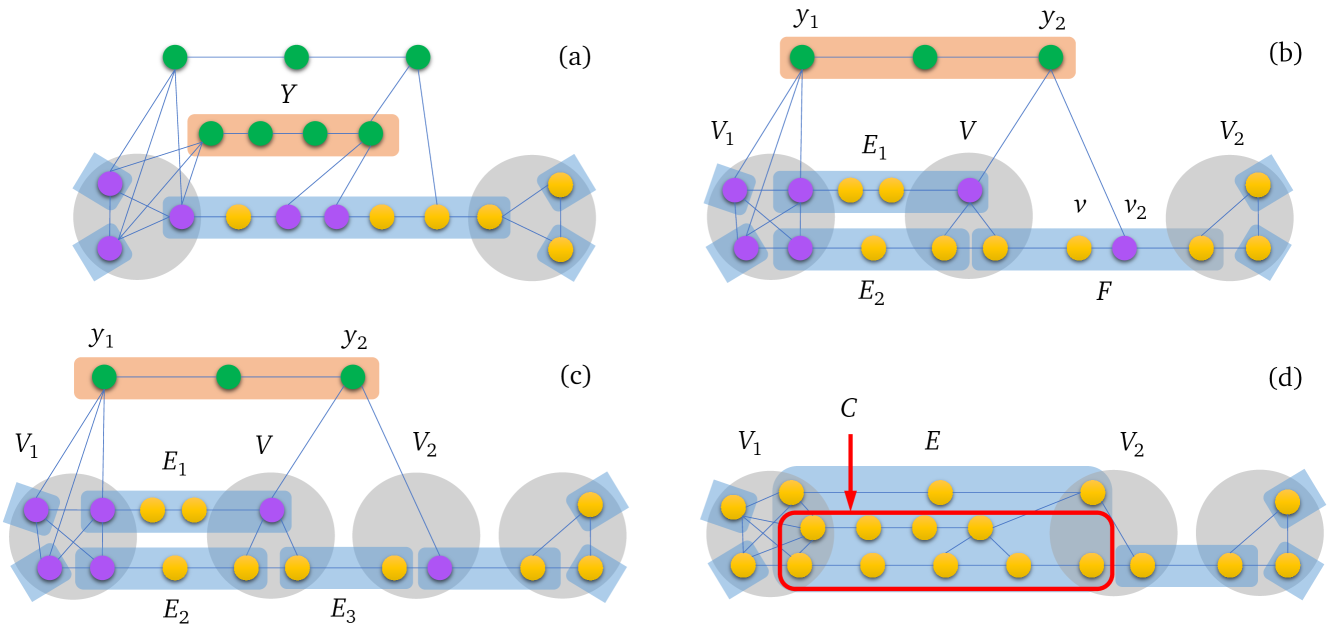
Figure 7: Applying Step BB1 on the example in (a) results in the example in (b), in which $E_{1}\cup E_{2}\cup F$ is a minimal pod of the green $y_{1}y_{2}$-rung. Applying Step B(B2)BB2(a) on the example in (b) results in the example in (c), in which $E_{1}\cup E_{2}\cup E_{3}$ is a minimal pod of the green $y_{1}y_{2}$-rung. Applying Steps B(B2)BB2(b) and B(B2)BB2(c) on the example in (c) results in the example in (d).

Proof of Lemma 3.2(2).

The resulting $\mathds{H}$ of Step BB1 is an $X\cup Y$-web, since all steps preserve Conditions N and all new arcs are simple. The rest of the proof shows that the resulting $\mathds{H}$ of Step BB2 is also an $X\cup Y$-web. At the beginning of Step B(B2)BB2(b) one can verify that, no matter whether $\mathds{H}$ is updated by Step B(B2)BB2(a) or not, $Y$ is $\mathds{H}$-nonsolid and $\mathds{H}$-podded and $\mathds{H}$ is an $X$-web with the following Condition F: If $V_{2}$ is incident to exactly one arc $F$ in the arc set for the minimal pod $C$ of $Y$ in $\mathds{H}$ and $F$ is simple, then $N(Y,V_{2})$ intersects $V_{2}\setminus C$. By Lemma 3.4, $\mathds{H}$ is an $X$-net (respectively, $X\cup Y$-net) at the end of Step B(B2)BB2(b) (respectively, Step B(B2)BB2(c)). It remains to show that $E=C\cup Y$ is a flexible arc by identifying an $(S,V_{1},V_{2})$-sprout of $G[E]$ for any nonempty subset $S$ of $E$. The rest of the proof lets $\mathds{H}$ denote the $X$-web at the beginning of Step B(B2)BB2(b) and lets all sprouts be $(S,V_{1},V_{2})$-sprouts of $G[E]$ unless specified otherwise. Let $y_{1}$ and $y_{2}$ be the end-vertices of path $G[Y]$ with $V_{1}\subseteq C\cup N(y_{1},X)$. If $|Y|=1$, then $y_{1}=y_{2}$. If $|Y|\geq 2$, then let $N_{i}=N(y_{i},X)$ and $M_{i}=N(Y\setminus\{y_{3-i}\},X)$ for each $i\in\{1,2\}$ and let $M=M_{1}\cap M_{2}$. Let $S_{C}=S\cap C$ and $S_{Y}=S\cap Y$. If $S_{C}\neq\varnothing$, then $S_{C}$ is assumed to be $\mathds{H}$-solid, since any $(S_{C},V_{1},V_{2})$-sprout of $G[C]$ is a sprout. If $S_{Y}\neq\varnothing$, then let each $P_{i}$ with $i\in\{1,2\}$ be the $Sy_{i}$-rung of $G[Y]$. Let $C^{*}=W_{1}W_{2}$ with $W_{1}=V_{1}$ be the arc of ${\mathds{H}\hskip 1.19995pt}^{\dagger}$ containing $C$.

Case 1: $S_{C}=\varnothing$. $G[S]$ is an edge in $G[Y]$ or else a $V_{1}V_{2}$-rung of $G[E]$ containing $Y$ contains a sprout of Type SS1 or SS2. By $|S|=2$, $|Y|\geq 2$. Since $Y$ is ${\mathds{H}\hskip 1.19995pt}^{\dagger}$-wild, $M_{1}\subseteq V_{1}$. We may assume $M_{1}=V_{1}$, since otherwise $G[P_{1}\cup Q]$ is a spout of Type SS3 for a $V_{1}V_{2}$-rung $Q$ of $G[C]$ intersecting $V_{1}\setminus M_{1}$. Case 1(a): $M_{2}$ is $\mathds{H}$-nonsolid. Lemma 4.1(2) implies an $(M_{2},W_{1},W_{2})$-sprout $T^{*}$ of $G[C^{*}]$. Let $T=G[T^{*}[C]\cup P_{2}]$. If $T^{*}$ is of Type SS1 or SS2, then $T$ contains a sprout of Type SS1. If $T^{*}$ is of Type SS3, then $T$ is a sprout of Type SS3. Case 1(b): $M_{2}$ is $\mathds{H}$-solid. Since $M_{1}$ is $\mathds{H}$-solid and $Y$ is $\mathds{H}$-nonsolid, we have $M\neq\varnothing$ and $M\subseteq V_{1}\cap M_{2}$. If $M_{2}$ were contained by a simple arc $F$ of $\mathds{H}$, then $F=V_{1}V_{2}$ by $V_{1}\cap M_{2}\neq\varnothing$ and minimality of $C$, contradicting Condition F. Thus, $M_{2}$ is a node of $\mathds{H}$. By $V_{1}\cap M_{2}\neq\varnothing$, $F=V_{1}M_{2}$ is an arc of $\mathds{H}$. By $M\subseteq V_{1}$, we have $M_{2}\subseteq F\cup N_{2}$. By minimality of $C$, $M_{2}=V_{2}$. By $M\neq\varnothing$ and $|Y|\geq 3$, $G[Y\cup M]$ contains a sprout of Type SS1.

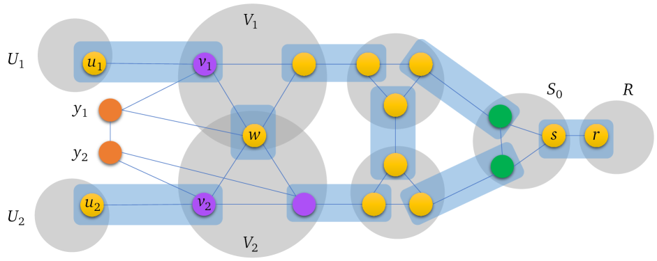
Figure 8: An example of $\mathds{H}_{0}$.

Case 2: $S_{Y}=\varnothing$. $S=S_{C}$ is $\mathds{H}$-solid. Let $v_{1}\in V_{1}\setminus C$, $v_{2}\in V_{2}\setminus C$, and a set of new vertices $B=\{r,s,u_{1},u_{2},w\}$. Define an $X_{0}$-net $\mathds{H}_{0}$ of a graph $G_{0}$ on $X_{0}\cup Y$ with $X_{0}=B\cup C\cup\{v_{1},v_{2}\}$ as follows (see Figure 8): Initially, let $G_{0}=G[C\cup Y\cup\{v_{1},v_{2}\}]$ and let $\mathds{H}_{0}$ consist of the nodes and arcs of $\mathds{H}$ that intersect $C$. For each $i\in\{1,2\}$, update $V_{i}$ by deleting all vertices not in $C$ except for $v_{i}$ and then adding $w$. Make a new simple arc $V_{1}V_{2}$ consisting of $w$. Add a minimum number of edges to make $N_{G_{0}}(w)=(\{y_{1}\}\cup V_{1}\cup V_{2})\setminus\{w\}$. Make new nodes $R=\{r\}$, $U_{1}=\{u_{1}\}$, and $U_{2}=\{u_{2}\}$. If $S$ is a node, then let $S_{0}=S$; otherwise, make a new node $S_{0}$ via $\textsc{subdivide}(S)$. Add $s$ into $S_{0}$. Make a simple arc $RS_{0}$ consisting of $r$ and $s$. For each $i\in\{1,2\}$, make a simple arc $U_{i}V_{i}$ consisting of vertices $u_{i}$ and $v_{i}$. Add a minimum number of edges to make $N_{G_{0}}(s)=R\cup S$, $N_{G_{0}}(r)=\{s\}$, $N_{G_{0}}(u_{1})=\{v_{1}\}$, and $N_{G_{0}}(u_{2})=\{v_{2}\}$.

$\mathds{H}_{0}$ is an $X_{0}$-net of $G_{0}$ with leaf nodes $R$, $U_{1}$, and $U_{2}$ and leaf vertices $r$, $u_{1}$, and $u_{2}$. Since $\mathds{H}$ is an $X$-web of $G$ and all new arcs of $\mathds{H}_{0}$ are simple, $\mathds{H}_{0}$ is an $X_{0}$-web of $G_{0}$. Since each $V_{i}$ with $i\in\{1,2\}$ is the neighbor of $U_{i}$ and $V_{1}V_{2}$ is an arc of $\mathds{H}_{0}$, $V_{1}$ is a maximal split node of $\mathds{H}_{0}$. Since $Y$ is ${\mathds{H}\hskip 1.19995pt}^{\dagger}$-wild, $Y$ is $\mathds{H}_{0}^{\dagger}$-wild. Since $Y$ is $\mathds{H}$-nonsolid, $\{w\}$ is not a pod of $Y$ in $\mathds{H}_{0}$ and $Y$ is $\mathds{H}_{0}$-nonsolid. Since node $S_{0}$ is adjacent to leaf $R$ in $\mathds{H}_{0}$, no $V_{1}V_{2}$-chunk of $\mathds{H}_{0}$ intersects $S_{0}$, implying no pod of $Y$ in $\mathds{H}_{0}$ that is a superset of $C$. The minimality of $C$ implies no pod of $Y$ in $\mathds{H}_{0}$ that is a proper subset of $C$. Thus, $Y$ is $\mathds{H}_{0}$-unpodded. Lemma 3.2(1) implies a sapling $T_{0}$ of $G_{0}$. $T_{0}-(B\cup\{v_{1},v_{2}\})$ is a sprout.

Case 3: $S_{Y}\neq\varnothing$ and $S_{C}\neq\varnothing$. $S_{C}$ is $\mathds{H}$-solid. Assume $S_{Y}=\{y_{2}\}$, since otherwise $G[P_{1}\cup Q]$ for an $S_{C}V_{2}$-rung $Q$ of $G[C]$ not intersecting $V_{1}$ is a sprout of Type SS2. Assume that any $N_{2}V_{2}$-rung $Q$ of $G[C]$ intersects $S_{C}$ exactly at its end-vertex in $N_{2}$, since otherwise $G[P_{1}\cup Q]$ contains a sprout of Type SS1 or SS2. Thus, each vertex $v\in C$ admits a $vV_{2}$-rung $Q(v)$ of $G[C]$ with $(V_{1}\cup S_{C})\cap V(Q(v))\subseteq\{v\}$: Assume for contradiction a $v\in C$ such that each $vV_{2}$-rung $Q(v)$ with $V_{1}\cap V(Q(v))\subseteq\{v\}$ intersects $S_{C}\setminus\{v\}$. If $S_{C}$ is a node $V$ of $\mathds{H}$, then graph $\mathds{G}(\mathds{C})-V$ is disconnected. If $S_{C}$ is contained by a simple arc $F$ of $\mathds{H}$, then graph $\mathds{H}[\mathds{C}]-\{V_{1},V\}$ is disconnected. Either way, the minimality of $C$ implies that $N_{2}$ intersects the connected component of $G[C]-S_{C}$ that intersects $V_{2}$, implying an $N_{2}(V_{2}\setminus S_{C})$-rung of $G[C]$, contradicting the above assumption.

Case 3(a): a vertex $v\in N_{2}\setminus S_{C}$. $Q(v)$ does not intersect $S_{C}$, so $G[Y\cup Q(v)]$ is a sprout of Type SS1. Case 3(b): a vertex $v\in S_{C}\setminus N_{2}$. $Q(v)$ does not intersect $N_{2}$ or else the $N_{2}V_{2}$-rung of $Q(v)$ does not intersect $S_{C}$ at its end-vertex in $N_{2}$, contradiction. Thus, $G[Y\cup Q(v)]$ is a sprout of Type SS2. Case 3(c): $N_{2}=S_{C}$. If $M_{1}\neq V_{1}$, then $G[P_{1}\cup Q(v_{1})]$ for a $v_{1}\in V_{1}\setminus M_{1}$ contains a sprout of Type SS3. If $M_{1}=V_{1}$, then $M$ contains a $v_{1}$, since $Y$ is $\mathds{H}$-nonsolid. We have $N=M_{1}\cup N_{2}$. $M_{1}$ and $N_{2}$ are both $\mathds{H}$-solid. Thus, $G[Y\cup Q(v_{1})]$ contains a sprout of Type SS1. ∎

This completes the proof of our characterization in Theorem 3.1 as well as Chudnovsky and Seymour’s characterization in Theorem 2.2. Subroutine B can be implemented to run in $O(m)$ time, so Steps A(A2)AA2(c) and A(A2)AA2(d) take $O(m)$ time. Steps AA1, A(A2)AA2(a), and A(A2)AA2(b) take $O(m)$ time. Since the set of vertices of $G$ in $\mathds{H}$ is enlarged by Step A(A2)AA2(d) and not affected elsewhere, Step AA2 halts in $O(n)$ iterations. Thus, Algorithm A can be implemented to run in $O(mn)$ time. To complete proving Theorem 1.1, it remains to implement Algorithm A to run in $O(m\log^{2}n)$ time in §5 using dynamic graph algorithms and other data structures.

5 Proving Lemma 3.3

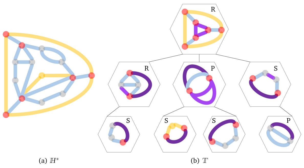
Figure 9: An example of ${\mathds{H}\hskip 1.00006pt}^{*}$ and $\mathds{T}$. The Q-knots are omitted for brevity. The virtual arc in dark purple in a nonroot knot $K$ matches a light purple arc in the parent of $K$ in $\mathds{T}$. They form the pair of virtual arcs between the poles of $K$. Each non-purple arc in a knot $K$ is a virtual arc whose corresponding arc of ${\mathds{H}\hskip 1.00006pt}^{*}$ is contained by a child Q-knot of $K$. A non-purple arc is in yellow if and only if its corresponding arc of ${\mathds{H}\hskip 1.00006pt}^{*}$ is dummy. The dummy nodes of ${\mathds{H}\hskip 1.00006pt}^{*}$ are in yellow. $\mathds{H}$ is the multigraph obtained from ${\mathds{H}\hskip 1.00006pt}^{*}$ by deleting the yellow nodes and arcs. ${\mathds{H}\hskip 1.19995pt}^{\dagger}$ is the simple graph obtained from the one in the root of $\mathds{T}$ by deleting the yellow arcs. The maximal split nodes of $\mathds{H}$, i.e., the nodes of ${\mathds{H}\hskip 1.19995pt}^{\dagger}$ are in red.

Let $G$ be represented by a static adjacency list. We use a dynamic adjacency list to represent an incremental biconnected multigraph ${\mathds{H}\hskip 1.00006pt}^{*}$ with $V({\mathds{H}\hskip 1.00006pt}^{*})=V(\mathds{H})$ that is a supergraph of $\nabla(\mathds{H})$. An arc or node of ${\mathds{H}\hskip 1.00006pt}^{*}$ is dummy if it is an empty vertex set of $G$. For instance, the three arcs of $\nabla(\mathds{H})$ between the leaves of $\mathds{H}$ are dummy in ${\mathds{H}\hskip 1.00006pt}^{*}$. Other dummy nodes and arcs are created only via operation merge. The $X$-web $\mathds{H}$ maintained by Algorithm A is exactly ${\mathds{H}\hskip 1.00006pt}^{*}$ excluding its dummy arcs and nodes. See Figure 9(a) for an example of ${\mathds{H}\hskip 1.00006pt}^{*}$. Each node and arc of $\mathds{H}$ and ${\mathds{H}\hskip 1.19995pt}^{\dagger}$ is associated with a distinct color that is a positive integer such that two vertices share a common arc color (respectively, node color) for $\mathds{H}$ and ${\mathds{H}\hskip 1.19995pt}^{\dagger}$ if and only if they are contained by a common arc (respectively, node) of $\mathds{H}$ and ${\mathds{H}\hskip 1.19995pt}^{\dagger}$. For each vertex $v$ of $G$, we maintain a set of at most six colors indicating the arc, maximal chunk, nodes, and maximal split nodes of $\mathds{H}$ that contain $v$, which are called the $\mathds{H}$-arc, ${\mathds{H}\hskip 1.19995pt}^{\dagger}$-arc, $\mathds{H}$-node, and ${\mathds{H}\hskip 1.19995pt}^{\dagger}$-node colors of vertex $v$. For each color $c$, we store its corresponding arc or node for $\mathds{H}$ or ${\mathds{H}\hskip 1.19995pt}^{\dagger}$ and maintain the number of the vertices having the color $c$ without keeping an explicit list of these vertices. For each node $V$ and each incident arc $E$ of $V$ in $\mathds{H}$, we maintain the cardinality of the vertex set $E\cap V$. Thus, it takes $O(1)$ time to (1) update and query the colors of a vertex and (2) add a vertex to an arc or node of $\mathds{H}$. For each arc of ${\mathds{H}\hskip 1.00006pt}^{*}$, we mark whether it is dummy, simple, or flexible and, for each simple arc $E=V_{1}V_{2}$ of ${\mathds{H}\hskip 1.00006pt}^{*}$, we use a doubly linked list to store the $V_{1}V_{2}$-rung $G[E]$. For any vertex $v$ and vertex set $Y$ of $G$, let $d(v)=|N(v)|$ and $d(Y)=\sum_{y\in Y}d(y)$ throughout the section.

Based on Lemma 5.1, to be proved in §5.4, Steps A(A2)AA2(a) and A(A2)AA2(b) are implemented in §5.1 to run in overall $O(m\log^{2}n)$ time throughout Algorithm A. Step A(A2)AA2(c) is implemented in §5.2 to run in overall $O(m)$ time throughout Algorithm A. Step A(A2)AA2(d), i.e., Subroutine B is implemented in §5.3 to run in overall $O(m\log n\cdot\alpha(n,n))$ time throughout Algorithm A, where $\alpha(n,n)$ is the inverse Ackermann function.

5.1 Steps A(A2)AA2(a) and A(A2)AA2(b) of Algorithm A

Although vertex colors change only in Step A(A2)AA2(d), the overall number of changes of the ${\mathds{H}\hskip 1.19995pt}^{\dagger}$-arc and ${\mathds{H}\hskip 1.19995pt}^{\dagger}$-node colors affects the analysis of our implementation of Steps A(A2)AA2(a) and A(A2)AA2(b). Therefore, this subsection analyzes the time for the change of ${\mathds{H}\hskip 1.19995pt}^{\dagger}$-arc and ${\mathds{H}\hskip 1.19995pt}^{\dagger}$-node colors. The time for the change of $\mathds{H}$-arc and $\mathds{H}$-node colors will be analyzed for Step A(A2)AA2(d) in §5.3. A vertex of $G$ stays uncolored until it is added into $X$. Each vertex of $X$ has exactly one ${\mathds{H}\hskip 1.19995pt}^{\dagger}$-arc color and at most two ${\mathds{H}\hskip 1.19995pt}^{\dagger}$-node colors. Each node $V$ of ${\mathds{H}\hskip 1.19995pt}^{\dagger}$ stays a node of ${\mathds{H}\hskip 1.19995pt}^{\dagger}$ and each vertex in $V$ stays in $V$ for the rest the algorithm. Thus, the ${\mathds{H}\hskip 1.19995pt}^{\dagger}$-node colors of each vertex are updated $O(1)$ times throughout the algorithm, implying that the overall time for updating ${\mathds{H}\hskip 1.19995pt}^{\dagger}$-node colors of all vertices is $O(n)$. Although the ${\mathds{H}\hskip 1.19995pt}^{\dagger}$-arc color of a vertex may change many times, the overall time for updating the ${\mathds{H}\hskip 1.19995pt}^{\dagger}$-node colors of all vertices can be bounded by $O(n\log n)$. Observe that $\mathds{H}$ is updated by Subroutine B only via (1) subdividing a simple arc of $\mathds{H}$, (2) merging an $\mathds{H}$-podded $Y$ into a minimal pod of $Y$ in $\mathds{H}$, and (3) creating an arc $E=Y$ for an $\mathds{H}$-solid $Y$. If the simple graph ${\mathds{H}\hskip 1.19995pt}^{\dagger}$ does not change, then each of these updates takes $O(d(Y))$ time. If the simple graph ${\mathds{H}\hskip 1.19995pt}^{\dagger}$ changes, then $Y$ is $\mathds{H}$-solid. For instance, let $\mathds{H}$ be as in Figure 5(a), implying that ${\mathds{H}\hskip 1.19995pt}^{\dagger}$ is as in Figure 5(b). If an $\mathds{H}$-solid $Y$ joins $\mathds{H}$ as the arc $E_{16}$ in Figure 5(c), then all nodes and arcs of $\mathds{H}$ become nodes and arcs of ${\mathds{H}\hskip 1.19995pt}^{\dagger}$. However, once two vertices of $X$ have distinct ${\mathds{H}\hskip 1.19995pt}^{\dagger}$-arc colors, they can no longer share a common arc color for ${\mathds{H}\hskip 1.19995pt}^{\dagger}$ for the rest of the algorithm. Thus, one can bound the overall number of changes of ${\mathds{H}\hskip 1.19995pt}^{\dagger}$-arc colors of all vertices by $O(n\log n)$ as follows: If $E$ is an arc of the original ${\mathds{H}\hskip 1.19995pt}^{\dagger}$ and $E_{1},\ldots,E_{k}$ are the arcs of the updated ${\mathds{H}\hskip 1.19995pt}^{\dagger}$ with $E_{1}\cup\cdots\cup E_{k}\subseteq E$ and $|E_{1}|\leq\cdots\leq|E_{k}|$, then let the vertices in $E_{k}$ keep their original ${\mathds{H}\hskip 1.19995pt}^{\dagger}$-arc color and assign a distinct new ${\mathds{H}\hskip 1.19995pt}^{\dagger}$-arc color to the vertices in each $E_{i}$ with $i\in\{1,\ldots,k-1\}$. Since the cardinality of the arc of ${\mathds{H}\hskip 1.19995pt}^{\dagger}$ containing a specific vertex of $X$ is halved each time its ${\mathds{H}\hskip 1.19995pt}^{\dagger}$-arc color changes, its ${\mathds{H}\hskip 1.19995pt}^{\dagger}$-arc color changes $O(\log n)$ times, implying that the ${\mathds{H}\hskip 1.19995pt}^{\dagger}$-arc colors of all vertices change $O(n\log n)$ times throughout the algorithm. With the data structure of Lemma 5.1, to be proved in §5.4, the overall time for Steps A(A2)AA2(a) and A(A2)AA2(b) throughout the algorithm is $O(m\log^{2}n)$.

Lemma 5.1.

If $X$ is an incremental subset of $V(G)$ such that each $x\in X$ has exactly one ${\mathds{H}\hskip 1.19995pt}^{\dagger}$-arc color $a$ and a set of at most two ${\mathds{H}\hskip 1.19995pt}^{\dagger}$-node colors corresponding to a subset of the two end-vertices of $a$, then there is an $O(m+n)$-time obtainable data structure supporting the following queries and updates:

1. Move a vertex $v$ of $G-X$ to $X$ in amortized $O(d(v)\cdot\log^{2}n)$ time.

2. Update the colors of a vertex $v\in X$ in amortized $O(d(v)\cdot\log n)$ time.

3. Determine if there is a set $Y\subseteq V(G-X)$ with connected $G[Y]$ such that two vertices of $N(Y,X)$ share no color and, for the positive case, report a minimal such $Y$ in amortized $O(d(Y)\cdot\log^{2}n)$ time.

5.2 Step A(A2)AA2(c) of Algorithm A

Let $\SS$ be the $O(d(Y))$-time obtainable set consisting of the nodes $V$ of $\mathds{H}$ with $V\subseteq N(Y,X)$ and the simple arcs $E$ of $\mathds{H}$ with $G[E\cap N(Y,X)]$ being an edge. $Y$ is $\mathds{H}$-solid if and only if $|\SS|=2$, $N(y,X)=\varnothing$ for each internal node $y$ of path $G[Y]$, and $N(Y,X)$ is contained by the union of the nodes or arcs in $\SS$. Therefore, it takes $O(d(Y))$ time to determine whether $Y$ is $\mathds{H}$-solid. Lemma 4.1(1) implies that $Y$ is $\mathds{H}$-podded if and only if both of the following conditions hold: (a) $N(Y,X)$ is contained by the union of an arc $E$ of ${\mathds{H}\hskip 1.19995pt}^{\dagger}$ and its end-nodes $V_{1}$ and $V_{2}$ in ${\mathds{H}\hskip 1.19995pt}^{\dagger}$ and (b) $E$ is a pod of $Y$ in ${\mathds{H}\hskip 1.19995pt}^{\dagger}$. Both conditions can be checked in $O(d(Y))$ time via the ${\mathds{H}\hskip 1.19995pt}^{\dagger}$-arc and ${\mathds{H}\hskip 1.19995pt}^{\dagger}$-node colors of each vertex in $N(Y,X)$ and the cardinalities of $V_{1}\setminus E$ and $V_{2}\setminus E$. Therefore, it takes $O(d(Y))$ time to determine whether $Y$ is $\mathds{H}$-podded. Since the ${\mathds{H}\hskip 1.19995pt}^{\dagger}$-wild sets $Y$ in all iterations of the algorithm are pairwise disjoint, it takes overall $O(m)$ time for Step A(A2)AA2(c) to determine whether $Y$ is $\mathds{H}$-sticky throughout the algorithm.

5.3 Step A(A2)AA2(d) of Algorithm A, i.e., Subroutine B

This subsection shows how to implement Subroutine B so that the overall time of Step A(A2)AA2(d) throughout Algorithm A is $O(m\log n\cdot\alpha(n,n))$. Although we may delete nodes and arcs from $\mathds{H}$ via $\textsc{merge}(C)$ for a minimal pod $C$ of $Y$ in $\mathds{H}$, they stay as dummy nodes and arcs in ${\mathds{H}\hskip 1.00006pt}^{*}$ in order to make the multigraph ${\mathds{H}\hskip 1.00006pt}^{*}$ incremental. One can verify that ${\mathds{H}\hskip 1.19995pt}^{\dagger}$ aids ${\mathds{H}\hskip 1.00006pt}^{*}$, even though ${\mathds{H}\hskip 1.00006pt}^{*}$ is not an $X$-net due to its dummy arcs and nodes. Although Step B(B1)BB1(b) may change ${\mathds{H}\hskip 1.19995pt}^{\dagger}$, the overall time for updating the ${\mathds{H}\hskip 1.19995pt}^{\dagger}$-colors has been accounted for in §5.1. Therefore, this subsection only analyzes the time required by the change of $\mathds{H}$-arc and $\mathds{H}$-node colors and the cardinalities of $E\cap V_{1}$ and $E\cap V_{2}$ for each arc $E=V_{1}V_{2}$ of $\mathds{H}$.

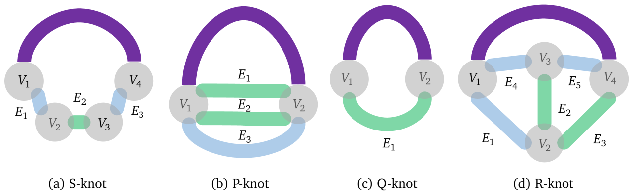
Figure 10: Four examples of the lowest common ancestor $K$ of the Q-knots containing the arcs of $\mathds{H}$ in $\mathds{C}_{1}\cup\mathds{C}_{2}$, which equals $E_{2}$ in (a), $E_{1}\cup E_{2}$ in (b), $E_{1}$ in (c), and $E_{2}\cup E_{3}$ in (d).

The SPQR-tree $\mathds{T}$ of the incremental multigraph ${\mathds{H}\hskip 1.00006pt}^{*}$ is an $O(n)$-time obtainable $O(n)$-space tree structure representing the triconnected components of ${\mathds{H}\hskip 1.00006pt}^{*}$ [45, 56]. Each member of $V(\mathds{T})$, which we call a knot, is a graph homeomorphic to a subgraph of ${\mathds{H}\hskip 1.00006pt}^{*}$ [45, Lemma 3] such that the knots induce a disjoint partition of the arcs of ${\mathds{H}\hskip 1.00006pt}^{*}$. Specifically, there is a supergraph $\mathds{G}$ of ${\mathds{H}\hskip 1.00006pt}^{*}$ with $V(\mathds{G})=V({\mathds{H}\hskip 1.00006pt}^{*})$, where each arc of $\mathds{G}\setminus{\mathds{H}\hskip 1.00006pt}^{*}$ is called virtual [80], and there are four types of knots of $\mathds{T}$: (1) S-knot: a simple cycle on three or more nodes. (2) P-knot: three or more parallel arcs. (3) Q-knot: two parallel arcs, exactly one of which is virtual. (4) R-knot: a triconnected simple graph that is not a cycle. The Q-knots are the leaves of $\mathds{T}$ and each arc of ${\mathds{H}\hskip 1.00006pt}^{*}$ is contained by a Q-knot. No two S-knots (respectively, P-knots) are adjacent in $\mathds{T}$. Each virtual arc is contained by exactly two adjacent knots. Since $\mathds{H}$ has $O(n)$ arcs by Condition NN2, $\mathds{T}$ has $O(n)$ knots. If $U$ and $V$ are nonleaf nodes of $\mathds{H}$ such that $UV$ is a virtual arc, then $\{U,V\}$ is a split pair of $\mathds{H}$. If distinct nodes $U$ and $V$ admit three internally disjoint $UV$-paths in ${\mathds{H}\hskip 1.00006pt}^{*}$, then $U$ and $V$ are contained by a common P-knot or R-knot of $\mathds{T}$ [45]. By Condition NN1 of $\mathds{H}$, there are three internally disjoint paths in $\nabla(\mathds{H})$ between each pair of leaves of ${\mathds{H}\hskip 1.00006pt}^{*}$, implying an R-knot of $\mathds{T}$ containing the leaves of $\mathds{H}$. Let $\mathds{T}$ be rooted at this unique R-knot. Figure 9(b) is the $\mathds{T}$ for the ${\mathds{H}\hskip 1.00006pt}^{*}$ in Figure 9(a). Let $K$ be a nonroot knot of $\mathds{T}$. The poles [56] of $K$ are the end-nodes of the unique virtual arc contained by $K$ and its parent knot in $\mathds{T}$. For the four nonroot knots $K$ in Figure 10, $V_{1}$ and $V_{4}$ (respectively, $V_{2}$) are the poles of the knots in (a) and (d) (respectively, (b) and (c)). Let $\mathds{C}(K)$ consist of the arcs of $\mathds{H}$ in the descendant Q-knots of $K$ in $\mathds{T}$. Let $C(K)$ consist of the vertices of $G$ contained by the arcs of $\mathds{C}(K)$. If $U$ and $V$ are the poles of a nonroot knot $K$ of $\mathds{T}$, then $C(K)$ is a $UV$-chunk and $\mathds{C}(K)$ is the arc set for $C(K)$. A nonempty vertex set $C$ is a maximal chunk of $\mathds{H}$ if and only if $C=C(K)$ holds for a child knot $K$ of the root of $\mathds{T}$. For instance, the $X$-net $\mathds{H}$ in Figure 9(a) has six maximal chunks. One of them is $C(K)$ for the child R-knot (respectively, P-knot and S-knot) $K$ of the root of $\mathds{T}$. The remaining three are $C(K)$ for three omitted child Q-knots $K$ of the root of $\mathds{T}$. For any nonroot knot $K$ of $\mathds{T}$ with $C(K)\neq\varnothing$, if $K$ is a P-knot, then $\mathds{C}(K)$ is the union of the arc sets of all split components of $\{U,V\}$ (e.g., three splits components of $\{V_{1},V_{2}\}$ in the example in Figure 10(b)); otherwise, $\mathds{C}(K)$ is the arc set of a single split component of $\{U,V\}$, where $U$ and $V$ are the poles of $K$ (e.g., exactly one split component for $\{V_{1},V_{4}\}$ in the examples in Figures 10(a) and 10(d) and exactly one split component for $\{V_{1},V_{2}\}$ in the example in Figure 10(c)).

Lemma 5.2 (Di Battista and Tamassia [45]).

Each update to $\mathds{T}$ corresponding to the following operations on the incremental biconnected multigraph ${\mathds{H}\hskip 1.00006pt}^{*}$ can be implemented to run in amortized $\alpha(n,n)$ time: (1) Add a new node $V$ to subdivide an arc $V_{1}V_{2}$ of ${\mathds{H}\hskip 1.00006pt}^{*}$ into two arcs $E_{1}=VV_{1}$ and $E_{2}=VV_{2}$. (2) Add an arc $UV$ between two nodes $U$ and $V$ of $\mathds{H}$.

We first show that, given a vertex set $S$ contained by a simple arc $E=V_{1}V_{2}$ such that $G[S]$ is an edge, Operation $\textsc{subdivide}(S)$ in Steps B(B1)BB1(a) and B(B2)BB2(a) can be implemented to run in amortized $O(\log n)$ time: Let each $P_{i}$ with $i\in\{1,2\}$ be the $V_{i}S$-rung of $G[E]$. Let $j$ be an index in $\{1,2\}$ with $|V(P_{j})|\leq|V(P_{3-j})|$. Using the doubly linked list for the $V_{1}V_{2}$-rung $G[E]$, it takes $O(|V(P_{j})|)$ time to (1) create a new node $V=S$ with a new $\mathds{H}$-node color assigned to both vertices in $S$, (2) create a new simple arc $E_{j}=VV_{j}$ consisting of the vertices of $P_{j}$, (3) assign a new $\mathds{H}$-arc color for each vertex in $E_{j}$, (4) let arc $E_{3-j}$ take over the $\mathds{H}$-arc color of $E$, and (5) obtain the doubly linked lists of $G[E_{1}]$ and $G[E_{2}]$ from that of $G[E]$. Each time a vertex $x$ is recolored this way, the cardinality of the simple arc of $\mathds{H}$ containing $x$ is halved. Therefore, the overall time for Operation $\textsc{subdivide}(S)$ in Steps B(B1)BB1(a) and B(B2)BB2(a) is $O(n\log n)$.

Step BB1: By the above analysis for subdivide, Step B(B1)BB1(a) runs in amortized $O(\log n)$ time. As for Steps B(B1)BB1(b) and B(B1)BB1(c), a new $\mathds{H}$-arc color is created for the new arc of $\mathds{H}$. The $\mathds{H}$-arc and $\mathds{H}$-node colors of the vertices in $Y$ and the cardinality of each vertex set that is a node, arc, or the intersection of a node and its incident arc can be updated in $O(d(Y))$ time. By Lemma 5.2 and the fact that Subroutine B is executed $O(n)$ times, the overall time for Step BB1 is $O(m\log n)$.

Step BB2: We first assume that we are given a set $\mathds{C}$ of arcs of $\mathds{H}$ whose union is a minimal pod $C$ of $Y$ in $\mathds{H}$ and show how to implement Steps B(B2)BB2(a), B(B2)BB2(b), and B(B2)BB2(c) to run in overall $O(m\log n)$ time throughout Algorithm A. Let $C$ be a $V_{1}V_{2}$-chunk of $\mathds{H}$.

Step B(B2)BB2(a): It takes $O(|\mathds{C}|)$ time to determine whether $V_{2}$ is incident to exactly one arc $F=VV_{2}$ in $\mathds{C}$ and $F$ is simple. We start from $V$ to traverse the $VV_{2}$-rung $G[F]$ to obtain the node $v_{2}\in N(Y,F)$ that is closest to $V_{2}$ in $G[F]$. The required time is linear in the number of traversed edges plus $d(Y)$. Observe that Step B(B2)BB2(a) in any remaining iteration of Algorithm A does not traverse these edges again. Moreover, the sum of $|\mathds{C}|$ over all iterations of Algorithm A is $O(n)$. Thus, the overall time of Step B(B2)BB2(a) including that of calling $\textsc{subdivide}(\{v,v_{2}\})$ is $O(m\log n)$.

Step B(B2)BB2(b): Let $E_{1},\ldots,E_{k}$ with $|E_{1}|\leq\cdots\leq|E_{k}|$ be the arcs of $\mathds{H}$ in $\mathds{C}$. We show how to implement Operation $\textsc{merge}(C)$ in Step B(B2)BB2(b) to run in amortized $O(\log n)$ time: We create a new arc $E=V_{1}V_{2}$ in ${\mathds{H}\hskip 1.00006pt}^{*}$ consisting of all vertices in $C$ and mark the original arcs $E_{1},\ldots,E_{k}$ of ${\mathds{H}\hskip 1.00006pt}^{*}$ intersecting $C$ dummy so that ${\mathds{H}\hskip 1.00006pt}^{*}$ is incremental as required by Lemma 5.2. The nodes of $\mathds{H}$ whose incident arcs are all dummy are also marked dummy. The cardinalities of $E$, $V_{1}$, $V_{2}$, $E\cap V_{1}$, and $E\cap V_{2}$ can be obtained in $O(k)$ time. Since we do not keep an explicit list of the vertices in $C$, we simply let all vertices in $C$ adopt the $\mathds{H}$-color of the vertices in $E_{k}$. Each time a vertex $v$ is recolored this way, the cardinality of the arc of $\mathds{H}$ containing $v$ is doubled. Observe that once a vertex in $X$ loses its $\mathds{H}$-node colors, it stays without any $\mathds{H}$-node color for the rest of the algorithm. Combining with Lemma 5.2(2), Step B(B2)BB2(b) takes overall $O(n\log n)$ time throughout Algorithm A.

Step B(B2)BB2(c): The $\mathds{H}$-arc and $\mathds{H}$-node colors of the vertices of $Y$ and the cardinalities of $E\cap V_{1}$ and $E\cap V_{2}$ can be updated in $O(d(Y))$ time.

Lemma 5.3 (Alstrup, Holm, Lichtenberg, and Thorup [3, §3.3]).

For any dynamic rooted $n$-knot tree, there is an $O(n)$-time obtainable data structure supporting the following operations and queries on $\mathds{T}$ in amortized $O(\log n)$ time for any given distinct knots $K_{1}$ and $K_{2}$ of $\mathds{T}$:

1. If $K_{2}$ is not a descendant of $K_{1}$, then make the subtree rooted at $K_{1}$ a subtree of $K_{2}$ such that $K_{2}$ becomes the parent of $K_{1}$.

2. Obtain the lowest common ancestor of $K_{1}$ and $K_{2}$.

3. If $K_{2}$ is a descendant of $K_{1}$, then obtain the child knot of $K_{1}$ that is an ancestor of $K_{2}$ in $\mathds{T}$.

It remains to show that it takes overall $O(m\log n\cdot\alpha(n,n))$ time to obtain the arc set $\mathds{C}$ of a minimal pod $C$ of an $\mathds{H}$-podded $Y$ in all iterations of Algorithm A. We additionally construct a data structure for $\mathds{T}$ ensured by Lemma 5.3. By Lemmas 5.2 and 5.3(1), the overall time for updating the data structure reflecting the updates to $\mathds{T}$ throughout algorithm A is $O(n\log n\cdot\alpha(n,n))$. Let $C^{*}=W_{1}W_{2}$ be the arc of ${\mathds{H}\hskip 1.19995pt}^{\dagger}$ with $V_{1}=W_{1}\subseteq N(Y,W_{1})\cup C^{*}$. By Conditions P, $C$ has to contain all arcs $E$ of $\mathds{H}$ with (1) $(E\setminus V_{1})\cap N(Y,X)\neq\varnothing$ or (2) $(E\cap V_{1})\setminus N(Y,X)\neq\varnothing$. Let $\mathds{C}_{1}$ and $\mathds{C}_{2}$ consist of the arcs of Types (1) and (2), respectively. It takes $O(d(Y))$ time to obtain $\mathds{C}_{1}$ and the incident arcs of $V_{1}$ that are not of Type (1) or (2). It then takes $O(|\mathds{C}_{2}|)$ time to obtain $\mathds{C}_{2}$. By Lemma 5.3(2), it takes $O(|\mathds{C}_{1}\cup\mathds{C}_{2}|\cdot\log n)$ time to obtain the lowest knot $K$ of $\mathds{T}$ with $\mathds{C}_{1}\cup\mathds{C}_{2}\subseteq\mathds{C}(K)$. Since all arcs in $\mathds{C}_{1}\cup\mathds{C}_{2}$ are merged into a single arc of $\mathds{H}$ via $\textsc{merge}(C)$ at the end of the current iteration, the overall time for obtaining $K$ throughout Algorithm A is $O(m\log n\cdot\alpha(n,n))$. It remains to show that $\mathds{C}$ can be obtained from $K$ in overall $O(m\log n\cdot\alpha(n,n))$ time throughout Algorithm A.

Case 1: $K$ is an S-knot. Let $V_{1}V_{2}\cdots V_{\ell}V_{1}$ with $\ell\geq 3$ be the cycle of $K$ such that $V_{1}$ and $V_{\ell}$ are the poles of $K$. For each $i\in\{1,\ldots,\ell-1\}$, let $K_{i}$ be the child knot of $K$ with poles $V_{i}$ and $V_{i+1}$, $\mathds{C}_{i}=\mathds{C}(K_{1})\cup\cdots\cup\mathds{C}(K_{i})$, and let $C_{i}$ be the union of the arcs in $\mathds{C}_{i}$. Let $j$ be the smallest index in $\{2,\ldots,\ell-1\}$ with $\mathds{C}_{1}\cup\mathds{C}_{2}\subseteq\mathds{C}_{j}$. If $N(Y,X)\setminus(V_{1}\cup C_{j-1})=V_{j}\setminus C_{j-1}$, then $\mathds{C}=\mathds{C}_{j-1}$; otherwise, $\mathds{C}=\mathds{C}_{j}$. For the example in Figure 10(a), if $N(X,Y)\setminus(V_{1}\cup E_{1})=V_{2}\setminus E_{1}$, then $E_{1}$ is a minimal pod of $Y$ in $\mathds{H}$; otherwise, $E_{1}\cup E_{2}$ is a minimal pod of $Y$ in $\mathds{H}$. By Lemma 5.3(3), the time required to obtain the index $j$ and determine whether $\mathds{C}=\mathds{C}_{j-1}$ or $\mathds{C}=\mathds{C}_{j}$ is dominated by the time of obtaining $K$ plus the time of $\textsc{merge}(C)$.

Case 2: $K$ is a P-knot. $\mathds{C}$ equals the union of $\mathds{C}(K^{\prime})$ over all child knots $K^{\prime}$ of $K$ in $\mathds{T}$ with $(\mathds{C}_{1}\cup\mathds{C}_{2})\cap\mathds{C}(K^{\prime})\neq\varnothing$. For the example in Figure 10(b), $E_{1}\cup E_{2}$ is a minimal pod of $Y$ in $\mathds{C}$. By Lemma 5.3(3), the time needed to obtain $\mathds{C}$ is dominated by that of obtaining $K$.

Case 3: $K$ is a Q-knot. As illustrated by Figure 10(c), $\mathds{C}=\mathds{C}(K)$ can be obtained in $O(1)$ time.

Case 4: $K$ is an R-knot. If there is child knot $K^{\prime}$ of $K$ in $\mathds{T}$ with poles $V_{1}$ and $V_{2}$ such that all arcs of $K$ intersecting $\mathds{C}_{1}\cup\mathds{C}_{2}$ are incident to $V_{2}$ and $N(Y,X)\setminus(V_{1}\cup C(K^{\prime}))=V_{2}\setminus C(K^{\prime})$, then $\mathds{C}=\mathds{C}(K^{\prime})$; otherwise, $\mathds{C}=\mathds{C}(K)$. For the example in Figure 10(d), if $N(Y,X)\setminus(V_{1}\cup E_{1})=V_{2}\setminus E_{1}$, then $E_{1}$ is a minimal pod of $Y$ in $\mathds{H}$; otherwise, $E_{1}\cup\cdots\cup E_{5}$ is a minimal pod of $Y$ in $\mathds{H}$. By Lemma 5.3(3), the time required to identify all possible vertices $V_{2}$, which can be at most two, is dominated by the time of identifying $K$. If there are no possible $V_{2}$, then we have $\mathds{C}=\mathds{C}(K)$. Otherwise, for each of the at most two vertices $V_{2}$, we spend $O(d(Y))$ time to determine whether the child knot $K^{\prime}$ with poles $V_{1}$ and $V_{2}$ satisfies $N(Y,X)\setminus(V_{1}\cup C(K^{\prime}))=V_{2}\setminus C(K^{\prime})$. For the positive (respectively, negative) case, we have $\mathds{C}=\mathds{C}(K^{\prime})$ (respectively, $\mathds{C}=\mathds{C}(K)$).

Therefore, the overall time for obtaining the arc set of a minimal pod of $Y$ in $\mathds{H}$ is $O(m\log n\cdot\alpha(n,n))$. To complete our proof of Lemma 3.3, it remains to prove Lemma 5.1 in §5.4.

5.4 Proving Lemma 5.1

The subsection omits ${\mathds{H}\hskip 1.19995pt}^{\dagger}$ from the terms ${\mathds{H}\hskip 1.19995pt}^{\dagger}$-wild, ${\mathds{H}\hskip 1.19995pt}^{\dagger}$-tamed, ${\mathds{H}\hskip 1.19995pt}^{\dagger}$-untamed, and ${\mathds{H}\hskip 1.19995pt}^{\dagger}$-node and ${\mathds{H}\hskip 1.19995pt}^{\dagger}$-arc colors. Recall that each vertex $x$ of $X$ is associated with exactly one arc color and at most two node colors from which we know which arc $E$ of ${\mathds{H}\hskip 1.19995pt}^{\dagger}$ contains $x$ and whether $x\in E\cap V$ holds for each end-node $V$ of $E$. For any nonempty $S\subseteq X$, we say that an $R\subseteq S$ represents $S$ and call $R$ a representative set of $S$ if $|R|\leq 3$ and, for any $V\subseteq X$, $R\cup V$ is tamed if and only if $S\cup V$ is tamed. If $S$ is untamed, then each untamed two-vertex subset of $S$ represents $S$. If $R_{1}$ represents $S_{1}$, $R_{2}$ represents $S_{2}$, and $R$ represents $R_{1}\cup R_{2}$, then $R$ represents $S_{1}\cup S_{2}$.

Lemma 5.4.

Any nonempty $S\subseteq X$ admits a representative set obtainable from the colors of the vertices of $S$ in $O(|S|)$ time.

Proof.

Let $E_{1},\ldots,E_{\ell}$ be the arcs of ${\mathds{H}\hskip 1.19995pt}^{\dagger}$ intersecting $S$. If $\ell=1$, then $S$ is tamed. Let $V_{1}$ and $V_{2}$ be the end-nodes of $E_{1}$. Choose an arbitrary vertex from each of the sets $S\cap V_{1}$, $S\cap V_{2}$, and $S\setminus(V_{1}\cup V_{2})$ that are nonempty to form a representative set of $S$. The rest of the proof assumes $\ell\geq 2$. It takes $O(|S|)$ time to either (1) identify distinct $i$ and $j$ in $\{1,\ldots,\ell\}$ such that $E_{i}$ and $E_{j}$ do not share a common end-node or (2) ensure that $E_{i}$ and $E_{j}$ for any distinct $i$ and $j$ in $\{1,\ldots,\ell\}$ share a common end-node. Case 1 implies that $S$ is untamed and any two-vertex subset of $S$ intersecting both $E_{i}$ and $E_{j}$ represents $S$.

Case 2(a): $E_{1},\ldots,E_{\ell}$ have a common end-node $V$. If $S\nsubseteq V$, then $S$ is untamed and any $\{u,v\}\subseteq S$ with $u\notin V$ intersecting distinct arcs represents $S$. If $S\subseteq V$, then $S$ is tamed. If $\ell=2$, then any two-vertex subset of $S$ intersecting both of $E_{1}$ and $E_{2}$ represents $S$. If $\ell\geq 3$, then any three-vertex subset of $S$ intersecting all of $E_{1}$, $E_{2}$, and $E_{3}$ represents $S$.

Case 2(b): $E_{1},\ldots,E_{\ell}$ have no common end-node. Therefore, $\ell=3$ and $E_{1}$, $E_{2}$, and $E_{3}$ form a triangle. For indices $i,j,k$ with $\{i,j,k\}=\{1,2,3\}$, let $V_{i}$ and $V_{j}$ be the end-nodes of $E_{k}$. If $S\subseteq\Delta(V_{1},V_{2},V_{3})$, then $S$ is tamed and any three-vertex subset of $S$ intersecting all of $E_{1}$, $E_{2}$, and $E_{3}$ represents $S$. If $S\nsubseteq\Delta(V_{1},V_{2},V_{3})$, then $S$ is untamed and $\{u,v\}$ with $u\in(S\cap E_{i})\setminus V_{j}$ and $v\in S\cap E_{k}$ for $\{i,j,k\}=\{1,2,3\}$ represents $S$. ∎

For each $y\in V(G-X)$, we maintain a balanced binary search tree $T_{y}$ on $N(y,X)$. For each vertex $x$ of $T_{y}$, we maintain a representative set $R_{y}(x)$ of the vertices in the subtree of $T_{y}$ rooted at $x$. Thus, $R_{y}=R_{y}(\text{root}(T_{y}))$ represents $N(y,X)$. We also maintain a doubly linked list $D_{1}$ for the vertices $y\in V(G-X)$ with untamed $N(y,X)$. When a vertex joins $N(y,X)$ or a vertex in $N(y,X)$ changes color, $R_{y}$ and $D_{1}$ can be updated in $O(\log n)$ time by Lemma 5.4. Thus, as long as $D_{1}\neq\varnothing$, ${\mathds{H}\hskip 1.19995pt}^{\dagger}$ is not taming and an ${\mathds{H}\hskip 1.19995pt}^{\dagger}$-wild set consisting of a single vertex can be obtained from $D_{1}$ in $O(1)$ time, implying Lemmas 5.1(1), 5.1(2), and 5.1(3). The rest of the subsection handles the case $D_{1}=\varnothing$.

Lemma 5.5 (Holm, de Lichtenberg, and Thorup [58]).

A spanning forest of an $n$-vertex dynamic graph can be maintained in amortized $O(\log^{2}n)$ time per edge insertion and deletion such that each update to the graph only adds and deletes at most one edge in the spanning forest.

We maintain a spanning forest $F$ of the decremental graph $G-X$ by Lemma 5.5. For each maximal connected $U\subseteq V(F)$, we maintain a balanced binary search tree $T_{U}$ on $U$. For each $y\in U$, we maintain a representative set $R_{U}(y)$ for the union of $R_{z}$ over all vertices $z$ in the subtree of $T_{U}$ rooted at $y$. It takes $O(1)$ time to determine if $U$ is tamed from $R_{U}=R_{U}(\text{root}(T_{U}))$. We also maintain a doubly linked list $D_{2}$ for the untamed maximal connected subsets $U$ of $V(F)$. When $R_{y}$ for a vertex $y\in V(G-X)$ changes, $D_{2}$ and $R_{U}$ for the maximal connected $U\subseteq V(F)$ containing $y$ can be updated in $O(\log n)$ time by Lemma 5.4. If deleting an edge of $F$ decomposes a maximal connected $U\subseteq V(F)$ into $U_{1}$ and $U_{2}$ with $|U_{1}|\leq|U_{2}|$, then it takes $O(|U_{1}|\log n)$ time to delete the vertices of $U_{1}$ from $T_{U}$, construct $T_{U_{1}}$, and obtain $R_{U_{1}}$. The resulting $T_{U}$ and $R_{U}$ become $T_{U_{2}}$ and $R_{U_{2}}$. $D_{2}$ can be updated in $O(1)$ time. Whenever a vertex $y$ moves to a new connected component, the number of vertices of the connected component containing $y$ is halved. Hence, the $T_{U}$ for all maximal connected sets $U\subseteq V(F)$ are changed overall $O(n\log n)$ times. Thus, the overall time throughout the algorithm to maintain $D_{2}$ and all representative sets $R_{U}$ is $O(n\log^{2}n)$, not affecting the correctness of Lemmas 5.1(1) and 5.1(2) and the first half of Lemma 5.1(3). It remains to prove the second half of Lemma 5.1(3) for the case $D_{1}=\varnothing$ and $D_{2}\neq\varnothing$, i.e., each $N(y,X)$ with $y\in V(G-X)$ is tamed and ${\mathds{H}\hskip 1.19995pt}^{\dagger}$ is not taming.

Figure 11: The cases of joining the child clusters $A$ and $B$ with $|\partial A|\geq|\partial B|$ into their parent cluster $C=A\cup B$ on a top tree. The first row shows the three cases with $|\partial A|=|\partial B|$. The second row shows the two cases with $|\partial A|>|\partial B|$. The vertex in $A\cap B$ is in purple. The vertices in $\partial C$ are in black. If $|\partial C|=2$, then the black line indicates $\Pi(C)$. If $|\partial A|=2$, then the red line indicates $\Pi(A)$. If $|\partial B|=2$, then the yellow line indicates $\Pi(B)$.

A top tree is defined over a dynamic tree $T$ and a dynamic set $\partial T$ of at most two vertices of $T$. For any subtree $C$ of $T$, $\partial C=\partial_{(T,\partial T)}C$ consists of the vertices of $C$ belonging to $\partial T$ or adjacent to $V(T)\setminus V(C)$. A cluster [3] of $(T,\partial T)$ is a subtree $C$ of $T$ with $|E(C)|\geq 1$ and $|\partial C|\leq 2$. If $|\partial C|=2$, then let $\Pi(C)$ denote the path of $T$ between the vertices of $\partial C$. If $|E(T)|=0$, then $(T,\partial T)$ admits no cluster and the top tree over $(T,\partial T)$ is empty. If $|E(T)|\geq 1$, then a top tree ${\mathcal{T}}$ over $(T,\partial T)$ is a binary tree on clusters of $(T,\partial T)$ such that (1) the root of ${\mathcal{T}}$ is the maximal cluster $T$ of $(T,\partial T)$, (2) the leaves of ${\mathcal{T}}$ are the edges of $T$, i.e., the minimal clusters of $(T,\partial T)$, and (3) the children $A$ and $B$ of any cluster $C$ of $(T,\partial T)$ on ${\mathcal{T}}$ are edge disjoint clusters of $(T,\partial T)$ with $C=A\cup B$ and $|V(A)\cap V(B)|=1$. Figure 11 illustrates all possible cases of joining child clusters $A$ and $B$ into their parent cluster $C$ on ${\mathcal{T}}$. If $|\partial A|=|\partial C|=2$, then $\Pi(A)\subseteq\Pi(C)$. Moreover, $\Pi(A)=\Pi(C)$ if and only if $|\partial B|\leq 1$. For each vertex $v\in V(T)\setminus\partial T$, let $C_{v}$ denote the lowest cluster of $(T,\partial T)$ on ${\mathcal{T}}$ with $v\in V(C_{v})\setminus\partial C_{v}$. If $|\partial C|=2$, then $v\in V(C)$ is an internal vertex of $\Pi(C)$ if and only if $|\partial A|=2$ holds for every cluster $A$ on the $CC_{v}$-path of ${\mathcal{T}}$. A top forest ${\mathcal{F}}$ over a forest $F$ consists of top trees, one for each maximal subtree of $F$. According to Lemma 5.5, each update to $F$ either deletes an edge of $F$ or adds an edge between two maximal subtrees of $F$. In addition to that, ${\mathcal{F}}$ also needs be modified if $\partial T$ for a maximal subtree $T$ of $F$ is updated. To accommodate each update to $F$ or $\partial T$, we modify ${\mathcal{F}}$ via a sequence of operations such that there can be temporary top trees ${\mathcal{T}}_{C}$ rooted at clusters $C$ that are not maximal subtrees of $F$. Specifically, ${\mathcal{F}}$ is modified via the following $O(1)$-time top-tree operations:

• Create or destroy a top tree on a single cluster that is an edge.

• Split a top tree ${\mathcal{T}}_{C}$ into the two immediate subtrees of ${\mathcal{T}}_{C}$ by deleting the root $C$.

• Merge top trees ${\mathcal{T}}_{A}$ and ${\mathcal{T}}_{B}$ with $|V(A)\cap V(B)|=1$ into a top tree ${\mathcal{T}}_{C}$ rooted at $C=A\cup B$.

Lemma 5.6 (Alstrup, Holm, de Lichtenberg, and Thorup [3]).

An $n$-vertex forest $F$ admits an $O(n)$-space top forest ${\mathcal{F}}$ consisting of $O(\log n)$-height top trees such that for any maximal subtree $T$ of $F$,

1. it takes $O(1)$ time to obtain on the top tree ${\mathcal{T}}$ for $T$ (a) the cluster $C_{v}$ for any $v\in V(T)\setminus\partial T$, (b) the parent of a nonroot cluster, (c) the children of a non-leaf cluster, and (d) $\partial C$ for a cluster $C$ and

2. it takes $O(\log n)$ time to identify a sequence of $O(\log n)$ top-tree operations with which ${\mathcal{F}}$ can be modified in $O(\log n)$ time with respect to (a) updating $\partial T$, (b) deleting an edge of $T$, or (c) adding an edge between $T$ and another maximal subtree of $F$.

We use Lemma 5.6 to maintain a top forest ${\mathcal{F}}$ over the spanning forest $F$ of $G-X$ maintained by Lemma 5.5. For each cluster $C$ on each nonempty top tree ${\mathcal{T}}$ of ${\mathcal{F}}$, we maintain a representative set $R_{C}$ of $N(V(C)\setminus\partial C,X)$. We first show that maintaining the representative sets $R_{C}$ does not affect the complexity of maintaining ${\mathcal{F}}$ stated in Lemma 5.6 and that of maintaining the colors of the vertices of $X$ stated in Lemmas 5.1(1) and 5.1(2). By Lemma 5.4, the following bottom-up update for a cluster $B$ on a top tree ${\mathcal{T}}$ of ${\mathcal{F}}$ takes $O(\log n)$ time: For each cluster $C$ on the $BT$-path of ${\mathcal{T}}$ from $B$ to $T$, if $C$ is an edge $uv$ of $T$, then an $R_{C}$ can be obtained from $R_{u}\cup R_{v}$ in $O(1)$ time; if $C$ is not an edge of $T$, then an $R_{C}$ can be obtained from $R_{C_{1}}\cup R_{C_{2}}\cup R_{c}$ in $O(1)$ time, where $C_{1}$ and $C_{2}$ are the children of $C$ on ${\mathcal{T}}$ and $c$ is the vertex in $V(C_{1})\cap V(C_{2})$. Hence, the initial $R_{C}$ for all clusters $C$ of all top trees ${\mathcal{T}}$ of ${\mathcal{F}}$ can be obtained in overall $O(m\log n)$ time by performing a bottom-up update for each leaf cluster of each top tree. With respect to each top-tree operation, the representative sets $R_{C}$ can be updated in $O(1)$ time: For destroy and split, we simply delete $R_{C}$ together with the root $C$ of ${\mathcal{T}}_{C}$. For create and merge, we just perform a bottom-up update for $C$ in $O(1)$ time. Thus, maintaining the representative sets $R_{C}$ does not affect the complexity of maintaining ${\mathcal{F}}$ stated in Lemma 5.6. If a vertex $v\in V(G-X)$ moves to $X$ or a vertex $v\in X$ changes color, we update $R_{C}$ for all $O(d(v)\log n)$ clusters $C$ with $v\in N(V(C)\setminus\partial C,X)$. Specifically, for each of the $O(d(v))$ vertices $y\in V(G-X)$ with $v\in N(y,X)$, we perform a bottom-up update for $C_{y}$ in $O(\log n)$ time. Thus, maintaining the representative sets $R_{C}$ does not affect the correctness of Lemmas 5.1(1) and 5.1(2).

The rest of the subsection proves the second half of Lemma 5.1(3) for the case $D_{1}=\varnothing$ and $D_{2}\neq\varnothing$ in two steps. Let $T=F[U]$ for an arbitrary $U$ kept in $D_{2}$. Step 1 calls $\textsc{tree-wild}(T)$ to obtain $\{u,w\}$ for distinct vertices $u$ and $w$ of $T$ such that the vertices of the $uw$-path of $T$ is a minimal untamed connected vertex set of $T$. Step 2 calls $\textsc{graph-wild}(\{u,w\})$ to obtain a minimal untamed set $Y$ such that $G[Y]$ is a $uw$-path of $G$.

Step 1: Let ${\mathcal{T}}$ be the top tree of ${\mathcal{F}}$ for $T$. For any cluster $C$ on ${\mathcal{T}}$, let $R_{\partial C}$ be the union of $R_{v}$ over the vertices $v\in\partial C$. Let $\textsc{closest}(S,C,c)$ for

• a tamed set $S\subseteq X$ with $|S|\leq 6$,

• a cluster $C$ on ${\mathcal{T}}$ with untamed $S\cup R_{C}\cup R_{\partial C}$, and

• a vertex $c\in\partial C$ such that $S\cup R_{c}$ is tamed

be the following $O(\log n)$-time recursive algorithm that outputs a $y\in V(C)$ such that

• $S\cup R_{y}$ is untamed and

• $S\cup R_{z}$ is tamed for every internal vertex $z$ of the $yc$-path of $T$:

If $C$ is an edge $bc$, then return $b$. If $C$ is not an edge, then let $C_{1}$ and $C_{2}$ be the children of $C$ and let $b$ be the vertex in $C_{1}\cap C_{2}$. If there is an $i\in\{1,2\}$ with $c\in\partial C_{i}$ such that $S\cup R_{C_{i}}\cup R_{\partial C_{i}}$ is untamed, then return $\textsc{closest}(S,C_{i},c)$. Otherwise, we have $b\neq c$ and that $S\cup R_{C_{i}}\cup R_{\partial C_{i}}$ is untamed for the index $i\in\{1,2\}$ with $c\notin\partial C_{i}$. Return $\textsc{closest}(S,C_{i},b)$.

Let $\textsc{tree-wild}(C)$ for a cluster $C$ on ${\mathcal{T}}$ with untamed $R_{C}\cup R_{\partial C}$ be the following recursive subroutine: If $C$ is an edge $uw$ of $T$, then return $\{u,w\}$. Otherwise, let $C_{1}$ and $C_{2}$ be the children of $C$ on ${\mathcal{T}}$. If there is an $i\in\{1,2\}$ with untamed $R_{C_{i}}\cup R_{\partial C_{i}}$, then return $\textsc{tree-wild}(C_{i})$. Otherwise, $R_{C}\cup R_{\partial C}$ is untamed and $R_{C_{1}}\cup R_{\partial C_{1}}$ is tamed. Let $c$ be the vertex in $V(C_{1})\cap V(C_{2})$. Call $\textsc{closest}(R_{C_{1}}\cup R_{\partial C_{1}},C_{2},c)$ to obtain in $O(\log n)$ time a $w\in V(C_{2})$ such that

• $R_{C_{1}}\cup R_{\partial C_{1}}\cup R_{w}$ is untamed and

• $R_{C_{1}}\cup R_{\partial C_{1}}\cup R_{v}$ is tamed for every internal vertex $v$ of the $wc$-path of $T$.

Call $\textsc{closest}(R_{w},C_{1},c)$ to obtain in $O(\log n)$ time a $u\in V(C_{1})$ such that

• $R_{w}\cup R_{u}$ is untamed and

• $R_{w}\cup R_{v}$ is tamed for every internal vertex $v$ of the $uc$-path of $T$.

Let $P$ be the $uw$-path of $T$. $V(P)$ is a minimally untamed subset of $V(T)$ that is connected in $T$: Let $u^{\prime}$ and $w^{\prime}$ be distinct vertices of $V(P)$ with $\{u^{\prime},w^{\prime}\}\neq\{u,w\}$ such that $R_{u^{\prime}}\cup R_{w^{\prime}}$ is untamed and $u^{\prime}$ is closer to $u$ than $w$ in $P$. Since $R_{C_{1}}\cup R_{\partial C_{1}}$ and $R_{C_{2}}\cup R_{\partial C_{2}}$ are both tamed, we have $u^{\prime}\in V(C_{1})\setminus\partial C_{1}$ and $w^{\prime}\in V(C_{2})\setminus\partial C_{2}$. Since $R_{C_{1}}\cup R_{\partial C_{1}}\cup R_{v}$ is tamed for every internal vertex $v$ of the $wc$-path of $T$ and $u^{\prime}\in V(C_{1})$, we have $w^{\prime}=w$. Since $R_{w}\cup R_{v}$ is tamed for every internal vertex $v$ of the $uc$-path of $T$, we have $u^{\prime}=u$.

Step 2: To obtain in $O(d(Y)\log n)$ time a set $Y$ such that $G[Y]$ is a $uw$-path of $G-X$, it suffices to show an $O(d(u)\log n)$-time subroutine $\textsc{jump}(u,w)$ returning for any distinct vertices $u$ and $w$ of $T$ the vertex $v\in N_{G}(u,V(P))$ that is closest to $w$ in the $uw$-path $P$ of $T$: With $Y=\{u\}$ initially, we repeatedly add $v=\textsc{jump}(u,w)$ into $Y$ and let $u=v$ until $v=w$. The subroutine $\textsc{jump}(u,w)$ starts with updating ${\mathcal{T}}$ for setting $\partial T=\{u,w\}$ in $O(\log n)$ time by Lemma 5.6(2). Recall that $U=N_{G}(u,V(P-w))$ consists of the vertices $v\in N_{G}(u)$ such that $|\partial B|=2$ holds for every cluster $B$ on the $TC_{v}$-path of ${\mathcal{T}}$. By Lemma 5.6(1), it takes $O(d(u)\log n)$ time for $\textsc{jump}(u,w)$ to obtain $U$ and the set $\mathcal{C}$ consisting of the clusters on the $TC_{v}$-path of ${\mathcal{T}}$ for all vertices $v\in U$. If $U=\varnothing$, then $\textsc{jump}(u,w)$ returns $w$, since $uw$ is an edge of $T$. If $U\neq\varnothing$, then $\textsc{jump}(u,w)$ returns $v=\textsc{next}(T,w)$, where $\textsc{next}(C,w)$ for a cluster $C\in\mathcal{C}$ and a vertex $w\in\partial C$ is the following $O(\log n)$-time recursive subroutine: If $w\in N_{G}(u)$, then $\textsc{next}(C,w)$ returns $w$. If $w\notin N_{G}(u)$, then $C$ is not an edge of $T$. Let $C_{1}$ and $C_{2}$ be the children of $C$ on ${\mathcal{T}}$ with $w\in\partial C_{2}\setminus\partial C_{1}$. Let $c$ be the vertex in $V(C_{1})\cap V(C_{2})$. If $C_{2}\in\mathcal{C}$, then $\textsc{next}(C,w)$ returns $\textsc{next}(C_{2},w)$; otherwise, $\textsc{next}(C,w)$ returns $\textsc{next}(C_{1},c)$.

6 Improved graph recognition and detection algorithms

Section 6.1 gives our algorithms for detecting thetas, pyramids, and beetles. Section 6.2 gives our algorithms for recognizing perfect graphs and detecting odd holes. Section 6.3 gives our algorithm for detecting even holes.

6.1 Improved theta, pyramid, and beetle detection

Each previous algorithm for detecting a family $\mathds{F}$ of graphs in $G$ via the three-in-a-tree algorithm identifies a set $\mathds{G}$ of a polynomial number of subgraphs $H$ of $G$, each associated with a set $L(H)$ of three terminals, such that $G$ is $\mathds{F}$-free if and only if each graph $H$ in $\mathds{G}$ does not admit an induced tree containing $L(H)$. In addition to Theorem 1.1, our improvement are obtained via exploiting that the graphs $H$ in $\mathds{G}$ need not be subgraphs of $G$. For instance, if $\mathds{F}$ are thetas, then Chudnovsky and Seymour [28] obtained a set $\mathds{G}$ of $O(n^{7})$ subgraphs of $G$. Each $H\in\mathds{G}$ with $L(H)=\{a_{1},a_{2},a_{3}\}$ is uniquely determined from vertices $b$, $b_{1}$, $b_{2}$, $b_{3}$, $a_{1}$, $a_{2}$, and $a_{3}$ of $G$ such that $bb_{1}$, $bb_{2}$, $bb_{3}$, $a_{1}b_{1}$, $a_{2}b_{2}$, and $a_{3}b_{3}$ are the distinct edges of $G[\{b,b_{1},b_{2},b_{3},a_{1},a_{2},a_{3}\}]$. We observe that the requirement that $a_{1}b_{1}$, $a_{2}b_{2}$, and $a_{3}b_{3}$ are the distinct edges of $G[\{a_{1},a_{2},a_{3},b_{1},b_{2},b_{3}\}]$ can be achieved by making the neighbors of each $b_{i}$ with $i\in\{1,2,3\}$ in $V(G)\setminus\{b,b_{1},b_{2},b_{3}\}$ a clique. As a result, each $H\in\mathds{G}$ is determined from four vertices $b$, $b_{1}$, $b_{2}$, and $b_{3}$ such that $bb_{1}$, $bb_{2}$, and $bb_{3}$ are the distinct edges of $G[\{b,b_{1},b_{2},b_{3}\}]$. Thus, there is a set $\mathds{G}$ of $O(n^{4})$ $n$-vertex graphs $H$ with $L(H)=\{b_{1},b_{2},b_{3}\}$ such that $G$ is theta-free if and only if each graph $H$ in $\mathds{G}$ does not admit an induced tree containing $L(H)$. An $n^{3}$-factor is reduced from the number of the three-in-a-tree problems to be solved in order to determine whether $G$ is theta-free. Beetle detection can be improved similarly. Improving the algorithm for pyramid detection needs additional care, since a pyramid has to contain exactly one triangle.

6.1.1 Proving Theorem 1.2

Theorem 1.2 is immediate from Theorem 1.1 and the next lemma.

Lemma 6.1.

Thetas in an $n$-vertex $m$-edge graph $G$ can be detected by solving the three-in-a-tree problem on $O(mn^{2})$ linear-time-obtainable $n$-vertex graphs.

Proof.

Observe that $H$ is a theta of $G$ if and only if there are vertices $b$, $b_{1}$, $b_{2}$, and $b_{3}$ of $H$ such that $bb_{1}$, $bb_{2}$, and $bb_{3}$ are the distinct edges of $G[\{b,b_{1},b_{2},b_{3}\}]$ and $H-b$ is an induced subtree of $G-b$ having exactly three leaves $b_{1}$, $b_{2}$, and $b_{3}$. See Figure 2(a). For each of the $O(mn^{2})$ choices of vertices $b$, $b_{1}$, $b_{2}$, and $b_{3}$ such that $bb_{1}$, $bb_{2}$, and $bb_{3}$ are the distinct edges in $G[\{b,b_{1},b_{2},b_{3}\}]$, let $G(b,b_{1},b_{2},b_{3})$ denote the graph that is $O(m+n)$-time obtainable from $G$ by (1) deleting $N[b]\setminus\{b_{1},b_{2},b_{3}\}$ and (2) adding edges to make the remaining vertices in each $N(b_{i})$ with $i\in\{1,2,3\}$ a clique. We show that $G$ admits a theta $H$ if and only if one of the $O(mn^{2})$ graphs $G^{*}=G(b,b_{1},b_{2},b_{3})$ admits an induced subtree $T^{*}$ containing $\{b_{1},b_{2},b_{3}\}$.

($\Rightarrow$) $G^{*}=G(b,b_{1},b_{2},b_{3})$ exists for the vertices $b$, $b_{1}$, $b_{2}$, and $b_{3}$ of $H$. The vertices deleted from $G$ in Step (1) are not in $T=H-b$, implying that $T$ is a subtree of $G^{*}$ containing $\{b_{1},b_{2},b_{3}\}$. Since $b_{1}$, $b_{2}$, and $b_{3}$ are the leaves of $T$, each edge added by Step (2) is incident to at most one vertex of $T$, implying that $T$ is an induced subtree $T^{*}$ of $G^{*}$ containing $\{b_{1},b_{2},b_{3}\}$.

($\Leftarrow$) The distinct edges of $G[\{b,b_{1},b_{2},b_{3}\}]$ are $bb_{1}$, $bb_{2}$, and $bb_{3}$. By Step (2), $b_{1}$, $b_{2}$, and $b_{3}$ are the leaves of $T^{*}$. Since each edge deleted in Step (1) is incident to at most one vertex of $T^{*}$, $T^{*}$ is an induced subtree of $G-b$, implying that $G[T^{*}\cup\{b\}]$ is a theta $H$ of $G$. ∎

6.1.2 Proving Theorem 1.3

A pyramid [28] of graph $G$ is the subgraph of $G$ induced by the vertices of an induced subtree $T$ of $G-\{b_{1}b_{2},b_{2}b_{3},b_{3}b_{1}\}$ having exactly three leaves $b_{1}$, $b_{2}$, and $b_{3}$ such that $G[\{b_{1},b_{2},b_{3}\}]$ is the only triangle of $G[T]$. See Figure 2(b). Theorem 1.3 is immediate from Theorem 1.1 and the next lemma.

Lemma 6.2.

Pyramids in an $n$-vertex $m$-edge graph $G$ can be detected by solving the three-in-a-tree problem on $O(mn)$ linear-time-obtainable $n$-vertex graphs.

Proof.

For each of the $O(mn)$ choices of distinct vertices $b_{1}$, $b_{2}$, and $b_{3}$ such that $G[\{b_{1},b_{2},b_{3}\}]$ is a triangle, let $G(b_{1},b_{2},b_{3})$ be the graph obtained from $G$ by (1) adding edges to make each $N(b_{i})\setminus\{b_{1},b_{2},b_{3}\}$ with $i\in\{1,2,3\}$ a clique, (2) deleting edges $b_{1}b_{2}$, $b_{2}b_{3}$, and $b_{3}b_{1}$, and (3) deleting $(N(b_{i})\cap N(b_{j}))\setminus\{b_{1},b_{2},b_{3}\}$ for any distinct indices $i$ and $j$ in $\{1,2,3\}$. We show that $G$ admits a pyramid $H$ if and only if one of the $O(mn)$ graphs $G^{*}=G(b_{1},b_{2},b_{3})$ admits an induced subtree $T^{*}$ containing $\{b_{1},b_{2},b_{3}\}$.

($\Rightarrow$) $G^{*}$ exists for the vertices $b_{1}$, $b_{2}$, and $b_{3}$ of $H$. Since $H[\{b_{1},b_{2},b_{3}\}]$ is the only triangle of $H$, $H$ does not intersect any $(N(b_{i})\cap N(b_{j}))\setminus\{b_{1},b_{2},b_{3}\}$ with $1\leq i<j\leq 3$. Hence, Steps (2) and (3) do not delete any edge of $T$, implying that $T$ is a subtree of $G^{*}$. Since $T$ is an induced tree of $G-\{b_{1}b_{2},b_{2}b_{3},b_{3}b_{1}\}$ having exactly three leaves $b_{1}$, $b_{2}$, and $b_{3}$, each edge added by Step (1) is incident to at most one vertex of $T$. Thus, $T$ is an induced subtree $T^{*}$ of $G^{*}$ containing $\{b_{1},b_{2},b_{3}\}$.

($\Leftarrow$) By Step (1), vertices $b_{1}$, $b_{2}$, and $b_{3}$ are the leaves of the subtree $T^{*}$ of $G$. Since each edge deleted in Step (3) is incident to at most one vertex of $T^{*}$, $T^{*}$ is an induced subtree of $G-\{b_{1}b_{2},b_{2}b_{3},b_{3}b_{1}\}$ by Step (2). By Steps (2) and (3), $G[\{b_{1},b_{2},b_{3}\}]$ is the only triangle of $G[T^{*}]$. Thus, $G[T^{*}]$ is a pyramid $H$ of $G$. ∎

6.1.3 Proving Theorem 1.5

A beetle [15] of graph $G$ is an induced subgraph of $G$ consisting of a cycle $b_{1}b_{2}b_{3}b_{4}b_{1}$ with a chord $b_{2}b_{4}$ (i.e., a diamond [36, 62] of $G$) and a tree $T$ of $G-b_{4}$ having exactly three leaves $b_{1}$, $b_{2}$, and $b_{3}$. See Figure 2(c). Theorem 1.5 is immediate from Theorem 1.1 and the next lemma.

Lemma 6.3.

Beetles in an $n$-vertex $m$-edge graph $G$ can be detected by solving the three-in-a-tree problem on $O(m^{2})$ linear-time-obtainable $n$-vertex graphs.

Proof.

For each of the $O(m^{2})$ choices of vertices $b_{1}$, $b_{2}$, $b_{3}$, and $b_{4}$ such that $G[\{b_{1},b_{2},b_{3},b_{4}\}]$ is a cycle $b_{1}b_{2}b_{3}b_{4}b_{1}$ with exactly one chord $b_{2}b_{4}$, let $G(b_{1},b_{2},b_{3},b_{4})$ be the $O(m+n)$-time obtainable graph from $G$ by (1) deleting $N[b_{4}]\setminus\{b_{1},b_{2},b_{3}\}$ and (2) adding edges to make the remaining vertices in each $N(b_{i})\setminus\{b_{1},b_{2},b_{3}\}$ with $i\in\{1,2,3\}$ a clique. We show that $G$ admits a beetle $H$ if and only if one of the $O(m^{2})$ graphs $G(b_{1},b_{2},b_{3},b_{4})$ admits an induced subtree $T^{*}$ containing $\{b_{1},b_{2},b_{3}\}$.

($\Rightarrow$) $G^{*}=G(b_{1},b_{2},b_{3},b_{4})$ exists for the vertices $b_{1}$, $b_{2}$, $b_{3}$, and $b_{4}$ of $H$. The vertices deleted fro $G$ in Step (1) are not in $T$, implying that $T$ is a subtree of $G^{*}$ containing $\{b_{1},b_{2},b_{3}\}$. Since $T$ intersects each $N(b_{i})\setminus\{b_{1},b_{2},b_{3}\}$ with $i\in\{1,2,3\}$ at exactly one vertex, each edge added by Step (2) is incident to at most one vertex of $T$. Thus, $T$ is an induced subtree $T^{*}$ of $G^{*}$ containing $\{b_{1},b_{2},b_{3}\}$.

($\Leftarrow$) $G[\{b_{1},b_{2},b_{3},b_{4}\}]$ is a cycle $b_{1}b_{2}b_{3}b_{4}b_{1}$ with exactly one chord $b_{2}b_{4}$. By Step (2), $b_{1}$, $b_{2}$, and $b_{3}$ are the leaves of $T^{*}$. Since each edge deleted in Step (1) is incident to at most one vertex of $T^{*}$, we have $G[T^{*}]=T^{*}\cup\{b_{1}b_{2},b_{2}b_{3}\}$, implying that $G[T^{*}\cup\{b_{4}\}]$ is a beetle $H$ of $G$. ∎

6.2 Improved perfect-graph recognition and odd-hole detection

As summarized by Maffray and Trotignon [68, §2], the algorithm of Chudnovsky et al. [18] consists of two $O(n^{9})$-time phases. The first phase (a) detects pyramids in $G$ in $O(n^{9})$ time, (b) detects the so-called $\mathcal{T}_{i}$ configurations with $i\in\{1,2,3\}$ in $O(n^{6})$ time, and (c) detects jewels in $\bar{G}$ in $O(n^{6})$ time. If any of them is detected, then either $G$ or $\bar{G}$ contains odd holes, implying that $G$ is not perfect. Otherwise, each shortest odd hole $C$ of $G$ is amenable, i.e., any anti-connected component of the $C$-major vertices is contained by $N_{G}(u)\cap N_{G}(v)$ for some edge $uv$ of $C$. The second phase (a) computes in $O(n^{5})$ time a set $\mathds{X}$ of $O(n^{5})$ subsets of $V(G)$ such that if $G$ contains an amenable shortest odd hole, then $\mathds{X}$ contains a near cleaner of $G$ and (b) spends $O(n^{4})$ time on each $X\in\mathds{X}$ to either obtain an odd hole of $G$ or ensure that $X$ is not a near cleaner of $G$. Theorem 1.3 reduces the time of detecting pyramids to $O(n^{6})$. Lemma 6.5 reduces the time of Phase 2(b) from $O(n^{4})$ to the time of performing $O(n)$ multiplications of Boolean $n\times n$ matrices [38, 64, 82]. Therefore, the time of recognizing perfect graphs is already reduced to $O(n^{8.377})$ without resorting to our improved odd-hole detection algorithm.

Let $G$ be an $n$-vertex $m$-edge graph. A $k$-hole (respectively, $k$-cycle and $k$-path) is a $k$-vertex hole (respectively, cycle and path). For any odd hole $C$ of $G$, a vertex $x\in V(G)\setminus V(C)$ is $C$-major [18] if $N_{G}(x,C)$ is not contained by any $3$-path of $C$. Let $M_{G}(C)$ consist of the $C$-major vertices. We have $M_{G}(C)\cap V(C)=\varnothing$. A shortest odd hole $C$ of $G$ is clean if $G$ does not contain any $C$-major vertex. A set $X\subseteq V(G)$ is a near cleaner [18] if there is a shortest odd hole $C$ of $G$ such that (1) $C[X]$ is contained by a $3$-path of $C$ and (2) all $C$-major vertices of $G$ are in $X$. A jewel of $G$ is an $O(n^{6})$-time detectable induced subgraph of $G$ [18]. If $G$ contains jewels or beetles, then $G$ contains odd holes. Let $\bar{G}$ denote the complement of graph $G$.

Lemma 6.4 (Chudnovsky, Cornuéjols, Liu, Seymour, and Vušković [18, 4.1]).

Let $u$ and $v$ be distinct vertices of a clean shortest odd hole $C$ of a pyramid-free jewel-free graph $G$. (1) The shortest $uv$-path of $C$ is a shortest $uv$-path of $G$. (2) The graph obtained from $C$ by replacing the shortest $uv$-path of $C$ with a shortest $uv$-path of $G$ remains a clean shortest odd hole of $G$.

6.2.1 An improved algorithm for recognizing perfect graphs

Although Theorem 1.4(1) implies Theorem 1.4(2), this subsection shows that we already have an improved algorithm for recognizing perfect graphs without resorting to Theorem 1.4(1). The next lemma reduces the time of Chudnovsky et al.’s algorithms [18, 4.2 and 5.1] from $O(n^{4})$ to $O(n^{3.377})$.

Lemma 6.5.

For any given vertex set $X$ of an $n$-vertex pyramid-free jewel-free graph $G$, it takes the time of performing $O(n)$ multiplications of $n\times n$ Boolean matrices to either obtain an odd hole of $G$ or ensure that $X$ is not a near cleaner of a shortest odd hole of $G$.

Proof.

It takes overall $O(n^{3})$ time to obtain for any distinct vertices $u$ and $v$ of $G$ that are connected in $G(u,v)=G-(X\setminus\{u,v\})$ (i) the length $d(u,v)$ of a shortest $uv$-path $P(u,v)$ in $G(u,v)$ and (ii) the neighbor $N(u,v)$ of $u$ in $P(u,v)$. Assume $P(u,v)=P(v,u)$ for all $u$ and $v$ without loss of generality. If $u$ and $v$ are not connected in $G(u,v)$, then let $d(u,v)=\infty$. It takes overall $O(n^{3})$ time to compute for any distinct vertices $x$ and $y$ of $G$ the set $Z(x,y)$ represented by an $n$-bit array, consisting of the vertices $z$ of $G$ with $d(z,x)=1$ and $d(z,y)>d(x,y)$. If

$$\begin{array}[]{rcl}d(x_{1},x_{2})&\geq&2\\ d(x_{1},y_{1})&=&d(x_{2},y_{2})\ \ =\ \ d(x_{1},y_{2})-1\ \ =\ \ d(x_{2},y_{1})-1\\ Z(x_{1},y_{1})\cap Z(x_{2},y_{2})&\neq&\varnothing\end{array}$$ (1)

with $y_{1}=N(y_{2},x_{1})$ hold for any distinct vertices $x_{1}$, $x_{2}$, and $y_{2}$ with minimum $d(x_{2},y_{2})$, then the $O(n^{2})$-time obtainable $C=G[P(x_{1},y_{1})\cup P(x_{2},y_{2})\cup\{z\}]$ for any $z\in Z(x_{1},y_{1})\cap Z(x_{2},y_{2})$ is an odd hole of $G$: Paths $P(x_{1},y_{1})$ and $P(x_{2},y_{2})$ are chordless. By $z\in Z(x_{1},y_{1})\cap Z(x_{2},y_{2})$, the only neighbors of $z$ in $C$ are $x_{1}$ and $x_{2}$. By $d(x_{1},x_{2})\geq 2$, $d(x_{i},y_{i})=d(x_{i},y_{3-i})-1$ for each $i\in\{1,2\}$, and the minimality of $d(x_{2},y_{2})$, the only edge between $P(x_{1},y_{1})$ and $P(x_{2},y_{2})$ is $y_{1}y_{2}$. Thus, $C$ is an odd hole of $G$. For each $y_{2}$, we construct a directed acyclic tripartite graph $G(y_{2})$ on three $n$-vertex sets $X_{1},Z,X_{2}$ such that (1) $x_{1}z$ with $x_{1}\in X_{1}$ and $z\in Z$ is a directed edge of $G(y_{2})$ if and only if $z\in Z(x_{1},N(y_{2},x_{1}))$ and (2) $zx_{2}$ with $z\in Z$ and $x_{2}\in X_{2}$ is a directed edge of $G(y_{2})$ if and only if $z\in Z(x_{2},y_{2})$. It takes the time of multiplying two $n\times n$ Boolean matrices to obtain the $O(n^{2})$ pairs of reachability in $G(y_{2})$ from $X_{1}$ to $X_{2}$. Thus, the time required to determine whether there is a choice of $x_{1}$, $x_{2}$, and $y_{2}$ satisfying Equation (1) is that of performing $O(n)$ multiplications for $n\times n$ Boolean matrices.

It remains to show that such a choice of $x_{1}$, $x_{2}$, and $y_{2}$ exists for the case that $X$ is a near cleaner of a shortest odd hole $C$ of $G$. Let $P$ be a $3$-path of $C$ such that $C-V(P)$ does not intersect the $C$-major vertices of $G$, implying that $C$ is a clean shortest odd hole of $H=G-(X\setminus V(P))$. Let $x_{1}$ and $x_{2}$ be the end-vertices of $P$. Let $y_{2}$ be the vertex of $C$ such that the shortest $x_{1}y_{2}$-path of $C$ is one edge longer than the shortest $x_{2}y_{2}$-path of $C$. By Lemma 6.4, each shortest $x_{i}y_{2}$-path $P_{i}$ of $C$ with $i\in\{1,2\}$ is a shortest $x_{i}y_{2}$-path of $H$. Since $X$ does not intersect the interior of $P_{1}$ and $P_{2}$, each $P(x_{i},y_{2})$ with $i\in\{1,2\}$ is a shortest $x_{i}y_{2}$-path of $H$. Applying Lemma 6.4(2) on $C$ to replace $P_{i}$ with $P(x_{i},y_{2})$ for each $i\in\{1,2\}$, we obtain a clean shortest odd hole $C^{*}$ of $H$, via which one can verify Equation (1) for the chosen $x_{1}$, $x_{2}$, and $y_{2}$: Let $y_{1}=N(y_{2},x_{1})$. Since $C^{*}$ is chordless in $G$, $d(x_{1},x_{2})\geq 2$. Since $X$ does not intersect the vertices of $C^{*}$ other than $x_{1}$, $x_{2}$, and the internal vertex $z$ of the shortest $x_{1}x_{2}$-path of $C^{*}$, we have $d(x_{1},y_{1})=d(x_{2},y_{2})=d(x_{1},y_{2})-1=d(x_{2},y_{1})-1$ by Lemma 6.4(1). We have $d(z,x_{1})=d(z,x_{2})=1$. By Lemma 6.4(1), $d(z,y_{i})>d(x_{i},y_{i})$ for both $i\in\{1,2\}$ or else the shortest $zy_{i}$-path of $C^{*}$ for an $i\in\{1,2\}$ would not be a shortest $zy_{i}$-path of $H$. Thus, $z\in Z(x_{1},y_{1})\cap Z(x_{2},y_{2})$. ∎

Lemma 6.6 (Chudnovsky, Cornuéjols, Liu, Seymour, and Vušković [18]).

Let $G$ be an $n$-vertex graph such that $G$ and $\bar{G}$ are pyramid-and-jewel-free. It takes $O(n^{6})$ time to (1) ensure that $G$ contains odd holes or (2) obtain a set $\mathds{X}$ of $O(n^{5})$ vertex subsets of $G$ such that if $G$ contains odd holes, then $\mathds{X}$ contains a near cleaner of $G$.

By Theorem 1.3, it takes $O(n^{6})$ time to detect pyramids or jewels in $G$ and $\bar{G}$. If $G$ or $\bar{G}$ contains pyramids or jewels, then $G$ is not perfect. By Lemma 6.6, it suffices to consider the case that we are given a set $\mathds{X}$ of $O(n^{5})$ vertex subsets such that if $G$ or $\bar{G}$ is not odd-hole-free, then $\mathds{X}$ contains a near cleaner of $G$ or $\bar{G}$. By Lemma 6.5, it takes overall $O(n^{8.377})$ time [38, 64, 82] to either obtain an odd hole of $G$ or $\bar{G}$ or ensure that both $G$ and $\bar{G}$ are odd-hole-free.

6.2.2 Proving Theorem 1.4

The recent odd-hole detection algorithm of Chudnovsky, Scott, Seymour, and Spirkl has seven $O(n^{9})$-time bottleneck subroutines. One is for pyramid detection, which is eliminated by Theorem 1.3. The remaining six are in two groups [26, §4]. The first (respectively, second) group handles the case that the longest $x$-gap (i.e., a path $D$ of $C$ such that $G[D\cup\{x\}]$ is a hole of $G$) over all $C$-major vertices $x$ for a shortest odd hole $C$ is shorter (respectively, longer) than one half of $C$. We give a two-phase algorithm to handle both cases in $O(n^{8})$ time. For the first case, Phase 1 tries all $O(n^{5})$ choices of five vertices to obtain an approximate cleaner for $C$, with which a shortest odd hole can be identified in $O(n^{3})$ time via Lemmas 6.5 and 6.8. For the second case, Phase 2 tries all $O(n^{6})$ choices of six vertices to obtain an approximate cleaner for $C$, with which a shortest odd hole can be identified in $O(n^{2})$ time via Lemma 6.9.

Lemma 6.7 (Chudnovsky, Scott, Seymour, and Spirkl [26, Theorem 3.4]).

Let $G$ be a jewel-free, pyramid-free, and $5$-hole-free graph. Let $C$ be a shortest odd hole in $G$. If $x\in M_{G}(C)$, then there is an edge of $C$ adjacent to each vertex of $M_{G}(C)\setminus N_{G}(x)$ in $G$.

A vertex set $X\subseteq V(G)$ is an approximate cleaner of $C$ if $X$ contains all $C$-major vertices and $X\cap V(C)\subseteq\{c_{1},c_{2}\}$ holds for two vertices $c_{1}$ and $c_{2}$ with $d_{C}(c_{1},c_{2})=3$. The second statement of the next lemma reduces the running time of an $O(n^{8})$-time subroutine of Chudnovsky et al. [26, Theorem 2.4] to $O(n^{5})$.

Lemma 6.8.

For any given vertex set $X$ of an $n$-vertex $m$-edge pyramid-free jewel-free $5$-hole-free graph $G$, (1) it takes $O(n^{3})$ time to obtain an odd hole of $G$ or ensure that $X$ is not an approximate cleaner of any shortest odd hole of $G$ and (2) it takes $O(mn^{3})$ time to either obtain an odd hole of $G$ or ensure that there is no shortest odd hole $C$ of $G$ such that an edge of $C$ is adjacent to all $C$-major vertices of $G$.

Proof.

We first show that Statement 1 implies Statement 2: For each edge $b_{1}b_{2}$ of $G$, we apply Statement 1 with $X=(N_{G}(b_{1})\cup N_{G}(b_{2}))\setminus\{b_{1},b_{2}\}$ in overall $O(mn^{3})$ time. If no odd hole is detected, then report that there is no shortest odd hole $C$ of $G$ such that an edge of $C$ is adjacent to all $C$-major vertices of $G$. To see the correctness, observe that if $C$ is a shortest odd hole of $G$ such that an edge $b_{1}b_{2}$ is adjacent to all $C$-major vertices of $G$, then $(N_{G}(b_{1})\cup N_{G}(b_{2}))\setminus\{b_{1},b_{2}\}$ is an approximate cleaner of $C$. Thus, Statement 2 holds.

It remains to prove Statement 1. It takes overall $O(n^{3})$ time to obtain for any distinct vertices $u$ and $v$ of $G$ that are connected in $G(u,v)=G-(X\setminus\{u,v\})$ (i) the length $d(u,v)$ of a shortest $uv$-path $P(u,v)$ in $G(u,v)$ and (ii) the neighbor $N(u,v)$ of $u$ in $P(u,v)$. Assume $P(u,v)=P(v,u)$ for all $u$ and $v$ without loss of generality. If $u$ and $v$ are not connected in $G(u,v)$, then let $d(u,v)=\infty$. It takes overall $O(n^{3})$ time to determine whether $C=G[P(c_{1},c_{2})\cup P(c_{1},b)\cup P(c_{2},b)]$ is a $7$-hole or the following equation holds for any distinct vertices $b$, $c_{1}$, and $c_{2}$ of $G$:

$$\begin{array}[]{rcl}d(c_{1},c_{2})&=&3\\ d(c_{1},N(c_{2},b))&>&3\\ d(c_{2},N(c_{1},b))&>&3\\ d(c_{1},b)&=&d(c_{2},b)\ \ =\ \ d(c_{1},N(b,c_{2}))-1\ \ =\ \ d(c_{2},N(b,c_{1}))-1.\end{array}$$ (2)

If Equation (2) holds for distinct vertices $b$, $c_{1}$, and $c_{2}$ with minimum $d(c_{1},b)$, then $C$ is an odd hole of $G$: Both $P(b,c_{1})$ and $P(b,c_{2})$ are chordless. By $d(c_{1},b)=d(c_{2},b)=d(c_{1},N(b,c_{2}))-1=d(c_{2},N(b,c_{1}))-1$ and the minimality of $d(c_{1},b)$, paths $P(b,c_{1})-b$ and $P(b,c_{2})-b$ are disjoint and nonadjacent. The interior of $P(c_{1},c_{2})$ is disjoint from and nonadjacent to $P((c_{1},b)-c_{1})\cup(P(c_{2},b)-c_{2})$, since otherwise $d(c_{i},N(c_{3-i},b))\leq 3$ or $d(c_{i},b)\geq d(c_{i},N(b,c_{3-i}))$ would hold for an $i\in\{1,2\}$. Thus, $C$ is an odd hole of $G$. It remains to show that if $X$ is an approximate cleaner for a shortest odd hole $C$ of $G$, then there is a choice of $b$, $c_{1}$, and $c_{2}$ such that Equation (2) holds or $C^{*}=G[P(c_{1},c_{2})\cup P(c_{1},b)\cup P(c_{2},b)]$ is a $7$-hole. Let $c_{1}$ and $c_{2}$ be two vertices of $C$ with $X\cap V(C)\subseteq\{c_{1},c_{2}\}$). Thus, $C$ is a clean shortest odd hole of $H=G-(X\setminus\{c_{1},c_{2}\})$. By $d_{C}(c_{1},c_{2})=3$, $|V(C)|\geq 7$, and Lemma 6.4, we have $d(c_{1},c_{2})=3$. Let $b$ be the vertex of $C$ with $d_{C}(b,c_{1})=d_{C}(b,c_{2})$. Apply Lemma 6.4 on $C$ to replace the shortest $bc_{1}$-path of $C$ with $P(b,c_{1})$, replace the shortest $bc_{2}$-path of $C$ with $P(b,c_{2})$, and replace the shortest $c_{1}c_{2}$-path of $C$ with $P(c_{1},c_{2})$. We obtain the clean shortest odd hole $C^{*}$ of $H$. Suppose $|V(C^{*})|\geq 9$. By $X\cap V(C)\subseteq\{c_{1},c_{2}\}$, $|V(C^{*})|\geq 9$, and Lemma 6.4, we have $d(c_{1},b)=d(c_{2},b)=d(c_{1},N(b,c_{2}))-1=d(c_{2},N(b,c_{2}))-1$. By Lemma 6.4 and $|V(C^{*})|\geq 9$, we have $d(c_{i},N(c_{3-i},b))>3$ for both $i\in\{1,2\}$. Thus, Equation (2) holds. ∎

Lemma 6.9.

Let $d$, $b_{1}$, and $b_{2}$ be distinct vertices of an $n$-vertex graph $G$. Let each $T_{i}$ with $i\in\{1,2\}$ be a subtree of $G-\{b_{1},b_{2}\}$ containing $d$. It takes $O(n^{2})$ time to determine whether there is a leaf $c_{i}$ of $T_{i}$ for each $i\in\{1,2\}$ such that if each $P_{i}$ with $i\in\{1,2\}$ is the $dc_{i}$-path of $T_{i}$, then $G[P_{1}\cup\{b_{1},b_{2}\}\cup P_{2}]$ is an odd hole of $G$.

Proof.

For each $i\in\{1,2\}$, let $T^{\prime}_{i}$ (respectively, $T^{\prime\prime}_{i}$) be the union of all $d$-to-leaf paths of $T_{i}$ with odd (respectively, even) lengths. In order for $G[P_{1}\cup\{b_{1},b_{2}\}\cup P_{2}]$ to be an odd hole, if $P_{1}$ is path of $T^{\prime}_{1}$ (respectively, $T^{\prime\prime}_{1}$), then $P_{2}$ is a path of $T^{\prime}_{2}$ (respectively, $T^{\prime\prime}_{2}$). Therefore, it suffices to work on the case that if each $c_{i}$ with $i\in\{1,2\}$ is a leaf of $T_{i}$, then (1) the union of path $c_{1}b_{1}b_{2}c_{2}$ and the $dc_{1}$-path $P_{1}$ of $T_{1}$ is an induced path of $G$, (2) the union of path $c_{1}b_{1}b_{2}c_{2}$ and the $dc_{2}$-path $P_{2}$ of $T_{2}$ is an induced path of $G$, and (3) $|E(P_{1})|+|E(P_{2})|$ is even. It remains to show how to determine in $O(n^{2})$ time whether there is an induced $c_{1}c_{2}$-path $P_{1}\cup P_{2}$. For each vertex $v$ of $T_{2}-d$, let set $S(v)$, implemented by an $n$-bit array associated with a counter for $|S(v)|$, be initially empty. Perform a depth-first traversal of $T_{1}$. When a vertex $u$ of $T_{1}-d$ is reached from its parent in $T_{1}$, insert $u$ into $S(v)$ for each vertex $v$ of $T_{2}-d$ with $u=v$ or $uv\in E(G)$ in overall $O(n)$ time. When the traversal is about to leave a vertex $u$ of $T_{1}-d$ for its parent in $T_{1}$, run the following $O(n)$-time steps: If $u$ is a leaf $c_{1}$ of $T_{1}$, then check whether there is a $dc_{2}$-path $P_{2}$ of $T_{2}$ for some leaf $c_{2}$ of $T_{2}$ such that $S(v)=\varnothing$ holds for all vertices $v$ of $P_{2}-d$. If there is such a $P_{2}$, then quit the traversal and report an odd hole $G[P_{1}\cup\{b_{1},b_{2}\}\cup P_{2}]$. If $u$ is not a leaf of $T_{1}$ or there is no such a $P_{2}$, then delete $u$ from $S(v)$ for each vertex $v$ of $T_{2}-d$ with $u\in S(v)$. If the traversal ends normally, then report negatively. The overall running time is $O(n^{2})$. To see the correctness, let $c_{1}$ be a traversed leaf of $T_{1}$. Let $c_{2}$ be an arbitrary leaf of $T_{2}$. Let each $P_{i}$ with $i\in\{1,2\}$ be the $dc_{i}$-path of $T_{i}$. Consider the moment when the traversal is about to leave $c_{1}$ for its parent in $T_{1}$. By the depth-first nature of the traversal, $S(v)\subseteq V(P_{1})$ holds for each vertex $v$ of $T_{2}-d$. Therefore, $P_{1}\cup P_{2}$ is an induced $c_{1}c_{2}$-path if and only if $S(v)=\varnothing$ holds for each vertex $v$ of $P_{2}-d$. ∎

Proof of Theorem 1.4.

It suffices to prove Statement 1. By Theorem 1.3 and Lemma 6.8(1), and the fact that jewels and $5$-holes are $O(n^{6})$-time detectable, we may assume that $G$ does not contain pyramids, jewels, $5$-holes, and clean shortest odd holes. By Lemma 6.8(2), we may further assume that $G$ does not contain any shortest odd hole $C$ such that an edge of $C$ is adjacent to all $C$-major vertices. The algorithm consists of two $O(m^{2}n^{4})$-time phases. If none of them identifies an odd hole of $G$, then report that $G$ is odd-hole-free. Let $x$, $d$, $d_{1}$, $d_{2}$, $c_{1}$, $b_{1}$, and $b_{2}$ be vertices of $G$ that are not necessarily distinct. Let

$$X_{1} = (N_{G}(b_{1})\cup N_{G}(b_{2}))\setminus\{b_{1},b_{2}\}$$

$$X_{2} = N_{G}(d_{1})\cap N_{G}(d_{2})$$

$$S_{0} = \{d_{1},d_{2}\}$$

$$S_{1} = \{d_{1},d_{2},c_{1}\}$$

$$S_{2} = \{d_{1},d_{2},c_{1},b_{1}\}.$$

For each $k\in\{0,1,2\}$, let

$$H_{k}=G-((X_{1}\cup N_{G}(x))\setminus S_{k}),$$

let $I_{k}$ consist of the internal vertices of all shortest $d_{1}d_{2}$-paths of $H_{k}$, let $J_{k}$ consist of vertex $d$ and the internal vertices of all shortest $dd_{1}$-paths and $dd_{2}$-paths of $H_{k}$, let $Y_{k}=N_{G}(x)\cap N_{G}(I_{k})$, and let $Z_{k}=N_{G}(x)\cap N_{G}(J_{k})$. If no odd hole of $G$ is identified via the following two phases, then report that $G$ is odd-hole-free.

Phase 1:

• For each of the $O(m^{2}n)$ choices of vertices $x,d_{1},d_{2},b_{1},b_{2}$ with $x\in N_{G}(d_{1})\cap N_{G}(d_{2})$ and $b_{1}b_{2}\in E(G)$, apply Lemma 6.8(1) with $X=(X_{1}\cup X_{2}\cup Y_{0})\setminus S_{0}$ in $O(n^{3})$ time.

• For each of the $O(m^{2}n)$ choices of vertices $x,c_{1},b_{1}=d_{1},b_{2},d_{2}$ with $x\in N_{G}(d_{1})\cap N_{G}(d_{2})$ and $b_{1}b_{2}\in E(G)$, apply Lemma 6.8(1) on $X=(X_{1}\cup X_{2}\cup Y_{1})\setminus S_{1}$ in $O(n^{3})$ time.

• For each of the $O(m^{2}n)$ choices of vertices $x,c_{1},b_{1},b_{2}=d_{1},d_{2}$ with $x\in N_{G}(d_{1})\cap N_{G}(d_{2})$ and $b_{1}b_{2}\in E(G)$, apply Lemma 6.8(1) on $X=(X_{1}\cup X_{2}\cup Y_{2})\setminus S_{2}$ in $O(n^{3})$ time.

Phase 2:

• For each of the $O(m^{2}n^{2})$ choices of vertices $x,d,d_{1},d_{2},b_{1},b_{2}$ with $x\in N_{G}(d_{1})\cap N_{G}(d_{2})$ and $b_{1}b_{2}\in E(G)$, apply the following procedure with $X=(X_{1}\cup X_{2}\cup Z_{0})\setminus S_{0}$ in $O(n^{2})$ time.

• For each of the $O(m^{2}n^{2})$ choices of vertices $x,d,c_{1},b_{1}=d_{1},b_{2},d_{2}$ with $x\in N_{G}(d_{1})\cap N_{G}(d_{2})$ and $b_{1}b_{2}\in E(G)$, apply the following procedure on $X=(X_{1}\cup X_{2}\cup Z_{1})\setminus S_{1}$ in $O(n^{2})$ time.

• For each of the $O(m^{2}n^{2})$ choices of vertices $x,d,c_{1},b_{1},b_{2}=d_{1},d_{2}$ with $x\in N_{G}(d_{1})\cap N_{G}(d_{2})$ and $b_{1}b_{2}\in E(G)$, apply the following procedure on $X=(X_{1}\cup X_{2}\cup Z_{2})\setminus S_{2}$ in $O(n^{2})$ time.

Let $C_{1}$ (respectively, $C_{2}$) consist of the vertices $c$ such that $cb_{1}b_{2}$ (respectively, $b_{1}b_{2}c$) is an induced path of $G$. Let $T^{*}_{1}$ be a tree that is the union of a shortest $dc$-path in $G-(X\setminus\{c,d\})$ over all vertices $c\in C_{1}$. Let each $T_{i}$ with $i\in\{1,2\}$ be a tree that is the union of a shortest $dd_{i}$-path and a shortest $d_{i}c$-path in $G-(X\setminus\{c,d\})$ over all vertices $c\in C_{i}$. Apply Lemma 6.9 on $d$, $b_{1}$, $b_{2}$, $T_{1}$ (respectively, $T^{*}_{1}$), and $T_{2}$ to identify an odd hole of $G$ in $O(n^{2})$ time.

The rest of the proof assumes that $C$ is a shortest odd hole of $G$ and shows that the above $O(m^{2}n^{4})$-time algorithm outputs an odd hole of $G$. Since $G$ does not contain any clean shortest odd hole, $M_{G}(C)\neq\varnothing$. For any $x\in M_{G}(C)$, a path $D$ of $C$ is an $x$-gap [26] if $G[D\cup\{x\}]$ is a hole of $G$. There is an $x\in M_{G}(C)$ with an $x$-gap or else each edge of $C$ would be adjacent to all vertices of $M_{G}(C)$. Let $x\in M_{G}(C)$ maximize the length of a longest $x$-gap $D$. Let $b_{1}b_{2}$ be an edge of $C$ adjacent to each vertex of $M_{G}(C)\setminus N_{G}(x)$ as ensured by Lemma 6.7, implying $M_{G}(C)\setminus X_{1}\subseteq N_{G}(x)$. Let $d_{1}$ and $d_{2}$ be the end-vertices of $D$. By the maximality of $D$, each vertex of $M_{G}(C)\setminus X_{2}$ is adjacent to the interior of $D$. Thus, each vertex of $M_{G}(C)\setminus(X_{1}\cup X_{2})$ is adjacent to $x$ and the interior of $D$. Let $c_{1}$ and $c_{2}$ be the vertices such that $c_{1}b_{1}b_{2}c_{2}$ is a path of $C$. We have $k=|V(D)\cap\{b_{1},b_{2}\}|\in\{0,1,2\}$. If $k=0$, then $S_{k}=\{d_{1},d_{2}\}$ and the interior of $D$ is disjoint from $c_{1}b_{1}b_{2}c_{2}$. If $k=1$, then assume without loss of generality $d_{1}=b_{1}$ and that $c_{1}$ is the neighbor of $d_{1}$ in $D$, implying $S_{k}=\{c_{1},b_{1}=d_{1},d_{2}\}$. If $k=2$, then assume without loss of generality $d_{1}=b_{2}$, by $x\in N_{G}(b_{1})\cup N_{G}(b_{2})$ and that $b_{1}$ is the neighbor of $d_{1}$ in $D$, implying $S_{k}=\{c_{1},b_{1},b_{2}=d_{1},d_{2}\}$.

For each $k\in\{0,1,2\}$, $D$ is a path of $H_{k}$: We have $N_{G}(x)\cap V(D)=\{d_{1},d_{2}\}\subseteq S_{k}$. By $X_{1}\cap V(D)=\{c_{1},c_{2}\}\cap V(D)\subseteq S_{k}$, we have $D\subseteq H_{k}$. By $M_{G}(C)\cap S_{k}=\varnothing$ and $M_{G}(C)\setminus X_{1}\subseteq N_{G}(x)$, we have $M_{G}(C)\subseteq(X_{1}\cup N_{G}(x))\setminus S_{k}$, implying $H_{k}\subseteq G-M_{G}(C)$.

Phase 1 handles the case $|E(D)|<0.5\cdot|E(C)|$: By Lemma 6.4(1), $D$ is a shortest $d_{1}d_{2}$-path of $G-M_{G}(C)$, implying that $D$ is a shortest $d_{1}d_{2}$-path of $H_{k}$. Since no edge of $C$ is adjacent to all $C$-major nodes of $G$, we have $|E(D)|\geq 3$ by the maximality of $D$. Thus, all internal vertices of $D$ are contained by $I_{k}$, implying $M_{G}(C)\setminus(X_{1}\cup X_{2})\subseteq Y_{k}$ by the maximality of $D$. Let $D^{*}$ be an arbitrary shortest $d_{1}d_{2}$-path of $H_{k}$. By $|E(D^{*})|=|E(D)|$ and $H_{k}\subseteq G-M_{G}(C)$, $D^{*}$ is a shortest $d_{1}d_{2}$-path of $G-M_{G}(C)$. By Lemma 6.4(2), the graph $C^{*}$ obtained from $C$ by replacing $D$ with $D^{*}$ is a clean shortest odd hole of $G-M_{G}(C)$. Therefore, the interior of $D^{*}$ is disjoint from and nonadjacent to $C-V(D)$, implying that $I_{k}$ is disjoint from and nonadjacent to $C-V(D)$. One can verify that $X=(X_{1}\cup X_{2}\cup Y_{k})\setminus S_{k}$ is either an approximate cleaner for $C$ with $X\cap V(C)=\{c_{1},c_{2}\}$ or $X\cap V(C)=\{c_{2}\}$. Thus, Phase 1 outputs an odd hole of $G$.

Phase 2 handles the case $|E(D)|>0.5\cdot|E(C)|$: Let $d$ be a middle vertex of $D$. For each index $i\in\{1,2\}$, the $dd_{i}$-path $D_{i}$ of $C$ is a shortest $dd_{i}$-path of $G-M_{G}(C)$ by Lemma 6.4(1), implying that $D_{i}$ is a shortest $dd_{i}$-path of $H_{k}$. Thus, all internal vertices of $D$ are contained by $J_{k}$, implying $M_{G}(C)\setminus(X_{1}\cup X_{2})\subseteq Z_{k}$. Let each $D^{*}_{i}$ with $i\in\{1,2\}$ be an arbitrary shortest $dd_{i}$-path of $H_{k}$. By $|E(D^{*}_{i})|=|E(D_{i})|$ and $H_{k}\subseteq G-M_{G}(C)$, $D^{*}_{i}$ is a shortest $dd_{i}$-path of $G-M_{G}(C)$. By Lemma 6.4(2), the graph $C^{*}$ obtained from $C$ by replacing $D$ with $D^{*}_{1}\cup D^{*}_{2}$ is a clean shortest odd hole of $G-M_{G}(C)$. Therefore, the interior of the $d_{1}d_{2}$-path $D^{*}_{1}\cup D^{*}_{2}$ is disjoint from and nonadjacent to $C-V(D)$, implying that $J_{k}$ is disjoint from and nonadjacent to $C-V(D)$. One can verify that $X=(X_{1}\cup X_{2}\cup Z_{k})\setminus S_{k}$ is an approximate cleaner for $C$ with $X\cap V(C)=\{c_{1},c_{2}\}$ or $X\cap V(C)=\{c_{2}\}$. We have $c_{1}\in C_{1}$ and $c_{2}\in C_{2}$.

• If $k=0$, then the $dc_{1}$-path $P_{1}$ of $T_{1}$ is the union of a shortest $dd_{1}$-path $P^{\prime}_{1}$ and a shortest $d_{1}c_{1}$-path $P^{\prime\prime}_{1}$ of $G-(X\setminus\{c_{1},d\})$ even if $c_{1}=d_{1}$. By $M_{G}(C)\subseteq X$, $X\cap V(C)\subseteq\{c_{1},c_{2}\}$, and the fact that the shortest $dd_{1}$-path and $d_{1}c_{1}$-path of $C$ are in $G-(X\setminus\{c_{1},d\})$, Lemma 6.4(1) implies that $P^{\prime}_{1}$ (respectively, $P^{\prime\prime}_{1}$) is a shortest $dd_{1}$-path (respectively, $d_{1}c_{1}$-path) of $G-M_{G}(C)$.

• If $k\in\{1,2\}$, then $c_{1}$ is an internal vertex of $D$. The $dc_{1}$-path $P_{1}$ of $T^{*}_{1}$ is a shortest $dc_{1}$-path of $G-(X\setminus\{c_{1},d\})$. By $M_{G}(C)\subseteq X$ and $X\cap V(C)=\{c_{2}\}$, Lemma 6.4(1) implies that $P_{1}$ is a shortest $dc_{1}$-path of $G-M_{G}(C)$.

The $dc_{2}$-path $P_{2}$ of $T_{2}$ is the union of a shortest $dd_{2}$-path $P^{\prime}_{2}$ and a shortest $d_{2}c_{2}$-path $P^{\prime\prime}_{2}$ of $G-(X\setminus\{c_{2},d\})$ even if $k=0$ and $c_{2}=d_{2}$. By $M_{G}(C)\subseteq X$, $X\cap V(C)\subseteq\{c_{1},c_{2}\}$, and the fact that the shortest $dd_{2}$-path and $d_{2}c_{2}$-path of $C$ are in $G-(X\setminus\{c_{2},d\})$, Lemma 6.4(1) implies that $P^{\prime}_{2}$ (respectively, $P^{\prime\prime}_{2}$) is a shortest $dd_{2}$-path (respectively, $d_{2}c_{2}$-path) of $G-M_{G}(C)$. By applying Lemma 6.4(2) at most four times on $C$, $G[P_{1}\cup\{b_{1},b_{2}\}\cup P_{2}]$ is a clean shortest odd hole of $G-M_{G}(C)$. Thus, Phase 2 outputs an odd hole of $G$. ∎

6.3 Improved even-hole detection

Chang and Lu’s algorithm consists of two $O(n^{11})$-time phases. The first phase detects beetles in $O(n^{11})$ time, which is now reduced to $O(n^{7})$ time by Theorem 1.5. The second phase maintains a set $\mathds{T}$ of induced subgraphs of $G$ with the property that if $G$ is even-hole-free, then so is each graph in $\mathds{T}$ until either $\mathds{T}$ becomes empty or an $H\in\mathds{T}$ is found to contain even holes. The initial $\mathds{T}$ consists of $O(n^{5})$ graphs obtained from guesses of (1) a $3$-path $P$ on a shortest even hole $C$ of $G$, (2) an $X\subseteq V(G)$ that contains the major vertices of $C$ without intersecting $C$, and (3) a $Y\subseteq V(G)$ that contains $N_{G}^{2,2}(C)$ (see §6.3.2 for definition) without intersecting $C$. Each iteration of Phase 2 takes $O(n^{4})$ time to either ensure that an $H\in\mathds{T}$ is an extended clique tree that contains even holes or replaces $H$ with $0$ (respectively, $1$ and $2$) smaller graphs via ensuring that $H$ is an even-hole-free extended clique tree (respectively, decomposing $H$ by a star-cutset and decomposing $H$ by a $2$-join). The guessed $P$ and $Y$ are crucial in arguing that $H$ can be decomposed by a star-cutset without increasing $|\mathds{T}|$, implying that each initial $H\in\mathds{T}$ incurs $O(n)$ decompositions by star-cutsets. Therefore, the overall time for decompositions by star-cutsets is $O(n^{10})$, i.e., $O(n^{5})$ times the initial $|\mathds{T}|$. Each initial $H\in\mathds{T}$ incurs $O(n^{2})$ decompositions by $2$-joins, implying that the overall time for detecting even holes in extended clique trees and decompositions by $2$-joins is $O(n^{11})$, i.e., $O(n^{6})$ times the initial $|\mathds{T}|$. We reduce the time of Phase 2 from $O(n^{11})$ to $O(n^{9})$. As in the proof of Lemma 6.10, a factor of $n$ is removed by reducing the initial $|\mathds{T}|$ from $O(n^{5})$ to $O(n^{4})$ via ignoring $Y$ and the internal vertex of $P$. Guessing only $X$ and the end-vertices of $P$ does complicate the task of decomposing $H$ by a star-cutset, but we manage to handle each decomposition by a star-cutset in the same time bound (see the proof of Lemma 6.11). Another factor of $n$ is removed by reducing the number of decompositions by $2$-joins incurred by each initial $H\in\mathds{T}$ from $O(n^{2})$ to $O(n)$ via carefully handling the boundary cases (see the proof of Lemma 6.12).

Let $G$ be an $n$-vertex $m$-edge graph. A major vertex [20] of an even hole $C$ is a $v\in V(G)\setminus V(C)$ with at least three distinct vertices in $N_{G}(v)\cap V(C)$ that are pairwise nonadjacent in $G$. Let $M_{G}(C)$ consist of the major vertices of an even hole $C$. A hole without major vertices is clear. A $v_{1}v_{2}$-hole of $G$ is a clear shortest even hole $C$ of $G$ such that $v_{1}$ and $v_{2}$ are the end-vertices of a $3$-path of $C$. A tracer of $G$ is a triple $\langle H,v_{1},v_{2}\rangle$ such that $v_{1}$ and $v_{2}$ are vertices of an induced subgraph $H$ of $G$. A tracer $\langle H,v_{1},v_{2}\rangle$ of $G$ is lucky if $H$ contains a $v_{1}v_{2}$-hole. A set $\mathds{T}$ of tracers of $G$ is reliable if $\mathds{T}$ satisfies the condition that if $G$ contains even holes, then $\mathds{T}$ contains lucky tracers.

Lemma 6.10.

If $G$ is beetle-free, then it takes $O(m^{2}n^{2})$ time to either ensure that $G$ contains even holes or obtain a reliable set of $O(mn^{2})$ tracers of $G$.

Subset $S$ of $V(H)$ is a star-cutset [31] of a graph $H$ if $S\subseteq N_{H}[s]$ holds for an $s\in S$ and the number of connected components of $H-S$ is more than that of $H$.

Lemma 6.11.

For any tracer $T$ of a beetle-free graph $G$, it takes $O(mn^{3})$ time to complete one of the following tasks. Task 1: ensure that $G$ contains even holes. Task 2: ensure that $T$ is not lucky. Task 3: obtain a star-cutset-free induced subgraph $H$ of $G$ such that if $T$ is lucky, then $H$ contains even holes.

The next lemma improves upon the $O(mn^{4})$-time algorithm of Chang and Lu. [15, Lemma 4.2].

Lemma 6.12.

It takes $O(mn^{3})$ time to detect even holes in an $n$-vertex $m$-edge star-cutset-free graph.

We first reduce Theorem 1.6 via Theorem 1.5 to Lemmas 6.10, 6.11, and 6.12.

Proof of Theorem 1.6.

By Theorem 1.5, it takes $O(m^{2}n^{3})$ time to detect beetles in $G$. If $G$ contains beetles, then $G$ contains even holes. Otherwise, we apply Lemma 6.10 on the beetle-free $G$ in $O(m^{2}n^{2})$ time. If $G$ is ensured to contain even holes, then the theorem is proved. Otherwise, we have a reliable set $\mathds{T}$ of $O(mn^{2})$ tracers of $G$. It takes overall $O(m^{2}n^{5})$ time to apply Lemma 6.11 on all $T\in\mathds{T}$. If Task 1 is completed for any $T\in\mathds{T}$, then $G$ contains even holes. If Task 2 is completed for all $T\in\mathds{T}$, then $G$ is even-hole-free. Otherwise, we apply Lemma 6.12 in overall $O(m^{2}n^{5})$ time on each of the $O(mn^{2})$ star-cutset-free induced subgraphs $H$ of $G$ corresponding to the tracers $T\in\mathds{T}$ for which Task 3 is completed. If an $H$ contains even holes, then so does $G$. Otherwise, $G$ is even-hole-free. ∎

Lemmas 6.10, 6.11, and 6.12 are proved in §6.3.1, §6.3.2, and §6.3.3, respectively.

6.3.1 Proving Lemma 6.10

Lemma 6.13 (da Silva and Vušković [40]).

Let $G$ be an $n$-vertex $m$-edge graph. It takes $O(mn^{2})$ time to either ensure that $G$ contains even holes or obtain all $O(m)$ maximal cliques of $G$.

Lemma 6.14 (Chang and Lu [15, Lemma 3.4]).

If $C$ is a shortest even hole of a $4$-hole-free graph $G$, then either $M_{G}(C)\subseteq N_{G}(v)$ holds for a vertex $v$ of $C$ or $G[M_{G}(C)]$ is a clique.

Proof of Lemma 6.10.

It takes $O(m^{2})$ time to detect $4$-holes in $G$, so we assume that $G$ is $4$-hole-free. By Lemma 6.13, it suffices to consider that the set $\mathds{K}$ of $O(m)$ maximal cliques of $G$ is available. It takes $O(m^{2}n^{2})$ time to obtain the set $\mathds{T}$ of $O(mn^{2})$ tracers of $G$ in the form of (1) $\langle G-(N_{G}(v)\setminus\{v_{1},v_{2}\}),v_{1},v_{2}\rangle$ with $\{v_{1},v,v_{2}\}\subseteq V(G)$ or (2) $\langle G-V(K),v_{1},v_{2}\rangle$ with $K\in\mathds{K}$ and $\{v_{1},v_{2}\}\subseteq V(G)$. To see that $\mathds{T}$ is reliable, let $C$ be a shortest even hole of $G$. Case 1: $M_{G}(C)\subseteq N_{G}(v)$ holds for a vertex $v$ of $C$. Let $v_{1}$ and $v_{2}$ be the neighbors of $v$ in $C$. By $M_{G}(C)\subseteq N_{G}(v)\setminus\{v_{1},v_{2}\}$ and $(N_{G}(v)\setminus\{v_{1},v_{2}\})\cap C=\varnothing$, $C$ is a $v_{1}v_{2}$-hole of $G-(N_{G}(v)\setminus\{v_{1},v_{2}\})$. Case 2: $M_{G}(C)\not\subseteq N_{G}(v)$ holds for all vertices $v$ of $C$. By Lemma 6.14, $G[M_{G}(C)]$ is a clique. Let $K$ be a maximal clique with $M_{G}(C)\subseteq V(K)$. We have $V(K)\cap C=\varnothing$ or else $M_{G}(C)\cap C=\varnothing$ would imply $M_{G}(C)\subseteq V(K)\setminus\{v\}\subseteq N_{G}(v)$ for any $v\in V(K)\cap C$, contradiction. Thus, $C$ is a $v_{1}v_{2}$-hole of $G-V(K)$ for any $v_{1}v_{2}$-path of $C$ with $3$ vertices. ∎

6.3.2 Proving Lemma 6.11

Vertex $x$ dominates vertex $y$ in graph $H$ if $x\neq y$ and $N_{H}[y]\subseteq N_{H}[x]$. Vertex $y$ is dominated in $H$ if some vertex of $H$ dominates $y$ in $H$. A star-cutset $S$ of graph $H$ is full if $S=N_{H}[s]$ holds for some vertex $s$ of $S$.

Lemma 6.15 (Chvátal [31, Theorem 1]).

A graph without dominated vertices and full star-cutsets is star-cutset-free.

Lemma 6.16 (Chudnovsky, Kawarabayashi, and Seymour [20, Lemma 2.2]).

If $x$ is a major vertex of a shortest even hole $C$ of graph $G$, then $|N_{G}(x,C)|$ is even.

Let $N_{G}^{i}(C)$ consist of the vertices $x\in N_{G}(C)\setminus M_{G}(C)$ such that $|N_{G}(x,C)|=i$ and $C[N_{G}(x,C)]$ is connected. Let $N_{G}^{i,i}(C)$ consist of the vertices $x\in N_{G}(C)\setminus M_{G}(C)$ such that $C[N_{G}(x,C)]$ has two connected components, each of which has $i$ vertices.

Lemma 6.17 (Chang and Lu [15, Lemma 2.2]).

For any clear shortest even hole $C$ of a beetle-free graph $G$, we have

$$N_{G}(C)\subseteq N_{G}^{1}(C)\cup N_{G}^{2}(C)\cup N_{G}^{3}(C)\cup N_{G}^{1,1}(C)\cup N_{G}^{2,2}(C).$$

Proof of Lemma 6.11.

We first prove the lemma using the following two claims for any tracer $T=\langle H,v_{1},v_{2}\rangle$ of an $n$-vertex $m$-edge beetle-free connected graph $G$:

1. It takes $O(mn^{2})$ time to obtain a tracer $T^{\prime}=\langle H^{\prime},v^{\prime}_{1},v^{\prime}_{2}\rangle$ of $G$, where $H^{\prime}$ is an induced subgraph of $H$ having no dominated vertices, such that if $T$ is lucky, then so is $T^{\prime}$.

2. It takes $O(mn^{2})$ time to (1) ensure that $H$ is full-star-cutset-free, (2) obtain an even hole of $G$, or (3) obtain a proper induced subgraph $H^{\prime}$ of $H$ such that if $T$ is lucky, then so is $\langle H^{\prime},v_{1},v_{2}\rangle$.

The algorithm proceeds in $O(n)$ iterations to update $T=\langle H,v_{1},v_{2}\rangle$. Each iteration starts with applying Claim 1 to update $T$ without destroying its luckiness by replacing $\langle H,v_{1},v_{2}\rangle$ with the ensured $\langle H^{\prime},v^{\prime}_{1},v^{\prime}_{2}\rangle$ such that $H^{\prime}$ is an induced subgraph of $H$ that does not contain any dominated vertex. It then applies Claim 2 on the resulting $T=\langle H,v_{1},v_{2}\rangle$. If $H$ is ensured to be full-star-cutset-free, then Task 3 is completed by Lemma 6.15. If we obtain an even hole of $G$, then Task 2 is completed. Otherwise, it updates $T$ without destroying its luckiness by replacing $H$ with the obtained proper induced subgraph $H^{\prime}$ of $H$ and proceed to the next iteration. The overall running time is $O(mn^{3})$.

To prove Claim 1, the $O(mn^{2})$-time algorithm outputs the resulting $T$ after iteratively updating the initial $T=\langle H,v_{1},v_{2}\rangle$ by the following procedure until $H$ contains no dominated vertices: (1) spend $O(mn)$ time to detect vertices $x$ and $y$ of $H$ such that $x$ dominates $y$ in $H$, (2) let $H=H-\{y\}$, and (3) if $y=v_{i}$ with $i\in\{1,2\}$, then let $v_{i}=x$. The resulting $H$ is an induced subgraph of the initial $H$. For the correctness, it suffices to prove that if a tracker $T$ is lucky, then so is the resulting $T$ after an iteration of the loop. Suppose that a $v_{1}v_{2}$-hole $C$ of $H$ contains $y$ or else $C$ remains a $v_{1}v_{2}$-hole of $H^{\prime}=H-\{y\}$. Since $C$ is an even hole, we have $x\notin V(C)$ and $|N_{C}[y]|=3$, implying a connected component of $C[N_{G}(x,C)]$ with at least $3$ vertices. By Lemma 6.17, we have $x\in N_{H}^{3}(C)$, implying that $N_{G}(x,C)$ consists of $y$ and the two neighbors of $y$ in $C$. Thus, $C^{\prime}=H[C\cup\{x\}\setminus\{y\}]$ remains a shortest even hole of $H^{\prime}$. Let $v_{0}$ be a vertex of $C$ such that $v_{1}v_{0}v_{2}$ is a $3$-path of $C$. For each $i\in\{0,1,2\}$, if $y=v_{i}$, then let $u_{i}=x$; otherwise, let $u_{i}=v_{i}$. Clearly, $u_{1}u_{0}u_{2}$ is a $3$-path of $C^{\prime}$. It remains to show that $C^{\prime}$ is clear. Assume for contradiction $z\in M_{H^{\prime}}(C^{\prime})$, implying $y\neq z$ and $z\in M_{H}(C^{\prime})$. By Lemma 6.16, $|N_{C^{\prime}}(z)|\geq 4$ and $|N_{C^{\prime}}(z)|\neq 5$. By Lemma 6.17, $M_{H}(C)=\varnothing$ implies $|N_{C}(z)|\leq 4$. By $C-\{y\}=C^{\prime}-\{x\}$, exactly one of $x$ and $y$ is adjacent to $z$ in $H$ or else $z\in M_{H}(C^{\prime})$ would imply $z\in M_{H}(C)$. Thus, $z\in N_{H}(x)\setminus N_{H}(y)$, implying $|N_{C}(z)|=|N_{C^{\prime}}(z)|-1=3$. Lemma 6.17 implies $z\in N_{H}^{3}(C)$. Since $C[N_{G}(z,C)]$ is a $3$-path, $H[C^{\prime}\cup\{z\}]$ is a beetle $B$ of $H$ in which $B[N_{B}[z]\setminus\{x\}]$ is a diamond, contradiction.

To prove Claim 2, it takes $O(mn)$ time to detect full star-cutsets in $H$. It suffices to focus on the case that $H$ contains a full star-cutset $S=N_{H}[s]$. Let $\mathds{B}$ consist of the connected components of $H-S$. It takes $O(n^{3})$ time to obtain, for every two nonadjacent vertices $s_{1}$ and $s_{2}$ of $S$, the list $L(s_{1},s_{2})$ of elements in $\mathds{B}$ that are adjacent to both $s_{1}$ and $s_{2}$. It takes $O(m^{2})$ time to check whether the following conditions hold:

1. There are distinct $B_{i}\in L(s_{1},s_{2})$ with $\{s_{1},s_{2}\}\subseteq S$ for $i\in\{1,2\}$.

2. There are disjoint edges $s_{i}s_{i+2}$ of $H[S]$ with distinct $B_{i}\in L(s_{2i-1},s_{2i})$ for $i\in\{1,2\}$.

If Condition 1 holds, then $H[P_{1}\cup P_{2}\cup s]$ (is a theta and thus) contains even holes for any shortest $s_{1}s_{2}$-path $P_{i}$ in $H[B_{i}\cup\{s_{1},s_{2}\}]$. If Condition 2 holds, then $H[P_{1}\cup P_{2}\cup s]$ contains even holes for any shortest $s_{2i-1}s_{2i}$-path $P_{i}$ in $H[B_{i}\cup\{s_{2i-1},s_{2i}\}]$. The rest of the proof assumes that neither condition holds. If there were a $v_{1}v_{2}$-hole $C$ of $H$ intersecting distinct $B_{1}$ and $B_{2}$ of $\mathds{B}$, then $s\notin C$, implying that $C[N_{G}(s,C)]$ is not connected. By Lemma 6.17, either $s\in N_{H}^{1,1}(C)$, implying Condition 1, or $s\in N_{H}^{2,2}(C)$, implying Condition 2. Hence, each $v_{1}v_{2}$-hole $C$ of $H$ intersects at most one element of $\mathds{B}$. If a $B\in\mathds{B}$ contains one or both of $v_{1}$ and $v_{2}$, then the claim is proved with $H^{\prime}=H[B\cup S]$. It remains to consider the case $\{v_{1},v_{2}\}\subseteq S$. Let $C$ be a $v_{1}v_{2}$-hole intersecting exactly one $B\in\mathds{B}$. If $s\in C$, then $V(C)\cap S=\{v_{1},s,v_{2}\}$, implying $B\in L(v_{1},v_{2})$. If $s\notin C$, then $s\in N_{H}^{3}(C)\cup N_{H}^{1,1}(C)\cup N_{H}^{2,2}(C)$ by Lemma 6.17, also implying $B\in L(v_{1},v_{2})$. Since Condition 1 does not hold, $|L(v_{1},v_{2})|\leq 1$. Therefore, if $|L(v_{1},v_{2})|=1$, then the claim is proved with $H^{\prime}=H[B\cup S]$, where $B$ is the only element in $L(v_{1},v_{2})$. If $|L(v_{1},v_{2})|=0$, then the claim is proved with $H^{\prime}=H[S]$. ∎

6.3.3 Proving Lemma 6.12

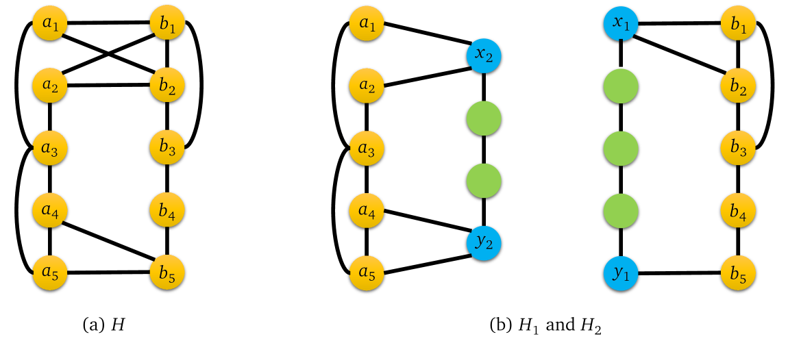
Figure 12: A $2$-join $J=(V_{1},V_{2},X_{1},X_{2},Y_{1},Y_{2})$ of $H$ with $V_{1}=\{a_{1},\ldots,a_{6}\}$, $V_{2}=\{b_{1},\ldots,b_{6}\}$, $X_{1}=\{a_{1},a_{2}\}$, $X_{2}=\{b_{1},b_{2}\}$ $Y_{1}=\{a_{5},a_{6}\}$, and $Y_{2}=\{b_{6}\}$ and and the parity-preserving blocks of decomposition $H_{1}$ and $H_{2}$ for $J$.

$(V_{1},V_{2},X_{1},X_{2},Y_{1},Y_{2})$ is a $2$-join [41, §1.3] (which is called a non-path $2$-join in, e.g., [15, 77, 79]) of a connected graph $H$ if

1. $V_{1}$ and $V_{2}$ form a disjoint partition of $V(H)$ with $|V_{1}|\geq 3$ and $|V_{2}|\geq 3$,

2. $X_{i}$ and $Y_{i}$ are disjoint nonempty subsets of $V_{i}$ for each $i$,

3. $H[V_{i}]$ is not a minimal $X_{i}Y_{i}$-path for each $i$, and

4. if $v_{i}\in V_{i}$ for each $i$, then $v_{1}v_{2}\in E(H)$ if and only if $v_{i}\in X_{i}$ for each $i$ or $v_{i}\in Y_{i}$ for each $i$.

See Figure 12(a) for an example.

Lemma 6.18 (Trotignon and Vušković [79, Lemma 3.2]).

If $(V_{1},V_{2},X_{1},Y_{1},X_{2},Y_{2})$ is a $2$-join of a star-cutset-free connected graph $H$, then the following statements hold for each $i\in\{1,2\}$:

1. Each connected component of $H[V_{i}]$ intersects both $X_{i}$ and $Y_{i}$.

2. Each vertex of $X_{i}$ (respectively, $Y_{i}$) has a non-neighbor of $H$ in $Y_{i}$ (respectively, $X_{i}$).

Lemma 6.19 (Charbit, Habib, Trotignon, and Vušković [17, Theorem 4.1]).

Given an $n$-vertex $m$-edge connected graph $H$, it takes $O(mn^{2})$ time to either obtain a $2$-join of $H$ or ensure that $H$ is $2$-join-free.

Lemma 6.20 (da Silva and Vušković [41, Corollary 1.3]).

A connected even-hole-free star-cutset-free $2$-join-free graph is an extended clique tree.

Let $J=(V_{1},V_{2},X_{1},X_{2},Y_{1},Y_{2})$ be a $2$-join of a star-cutset-free connected graph $H$. Let $P_{i}$ with $i\in\{1,2\}$ be a shortest induced $X_{i}Y_{i}$-path $P_{i}$ of $H[V_{i}]$ as ensured by Lemma 6.18(1). If $|V(P_{i})|$ is even (respectively, odd), then let $p_{i}=4$ (respectively, $p_{i}=5$). The parity-preserving blocks of decomposition [79] for $J$ are the graphs $H_{i}$ with $i\in\{1,2\}$ consisting of $H[V_{i}]$, a $p_{j}$-vertex $x_{j}y_{j}$-path with $j=3-i$, edges $xx_{j}$ for all vertices $x$ of $X_{i}$, and edges $yy_{j}$ for all vertices $y$ of $Y_{i}$. See Figure 12(b) for an example.

Lemma 6.21 (Trotignon and Vušković [79, Lemma 3.8]).

Let $H_{1}$ and $H_{2}$ be the parity-preserving blocks of decomposition for a $2$-join of an $m$-edge star-cutset-free connected graph $H$.

1. Both $H_{1}$ and $H_{2}$ are star-cutset-free.

2. Both $H_{1}$ and $H_{2}$ are even-hole-free if and only if $H$ is even-hole-free.

Lemma 6.22 (Chang and Lu [15, Lemma 4.12]).

Each of the parity-preserving blocks of decomposition for a $2$-join for an $n$-vertex $m$-edge star-cutset-free connected graph has at most $n$ vertices and $m$ edges.

Graph $H$ is an extended clique tree [41] if there is a set $S$ of two or fewer vertices of $H$ such that each biconnected component of $H-S$ is a clique. It takes $O(mn^{2})$ time to determine whether an $n$-vertex $m$-edge graph is an extended clique tree.

Lemma 6.23 (Chang and Lu [15, Lemma 4.6]).

It takes $O(n^{4})$ time to detect even holes in an $n$-vertex connected extended clique tree.

Proof of Lemma 6.12.

Let $W(H)$ consist of the $v\in V(H)$ with $|N_{H}(v)|\geq 3$. Let $h(H)=|V(H)|+|W(H)|$. We first prove the claim that if $H_{1}$ and $H_{2}$ are the parity-preserving blocks of decomposition for a $2$-join $(V_{1},V_{2},X_{1},X_{2},Y_{1},Y_{2})$ of a star-cutset-free connected graph $H$, then (a) $X_{i}\cup V_{j}$, $Y_{i}\cup V_{j}$, or $X_{i}\cup Y_{i}\cup V_{j}$ with $\{i,j\}=\{1,2\}$ induces a $6$-hole of $H$ or (b) we have

$$h(H_{1})+h(H_{2}) \leq h(H)+14$$ (3)

$$\max\{h(H_{1}),h(H_{2})\} \leq h(H)-1.$$ (4)

By definition of $H_{i}$ and $H_{j}$ with $\{i,j\}=\{1,2\}$, (i) if $v\in V_{i}$, then $|N_{H_{i}}(v)|\leq|N_{H}(v)|$, (ii) if $x_{j}\in W(H_{i})$, then $X_{j}\subseteq W(H)$, and (iii) if $y_{j}\in W(H_{i})$, then $Y_{j}\subseteq W(H)$. Thus, $|W(H_{i})|\leq|W(H)|$. By Lemma 6.22, $h(H_{i})\leq h(H)$. By $|V(H_{i})|=|V_{i}|+p_{j}\leq|V_{i}|+5$ and $W(H_{i})\setminus W(H)\subseteq\{x_{j},y_{j}\}$, Equation (3) holds. To see Equation (4), assume $h(H_{i})=h(H)$, implying

$$|V(H_{i})| = |V(H)|$$ (5)

$$|W(H_{i})| = |W(H)|.$$ (6)

By $|V(H_{i})|=|V(H)|-|V_{j}|+p_{j}$ and Equation (5), $|V_{j}|=p_{j}$. If $|V(P_{j})|\in\{4,5\}$, then $|V_{j}|=p_{j}=|V(P_{j})|$ contradicts $H[V_{j}]\neq P_{j}$. By $p_{j}\in\{4,5\}$, we have $|V(P_{j})|\in\{2,3\}$.

Case 1: $|V(P_{j})|=2$. $|V_{j}|=p_{j}=4$. By Lemma 6.18(2), $|X_{j}|=|Y_{j}|=2$. Thus, $|X_{i}|=|Y_{i}|=1$ or else $X_{j}\subseteq W(H)$ or $Y_{j}\subseteq W(H)$, contradicting Equation (6). Hence, $|N_{H_{i}}(x_{j})|=|N_{H_{i}}(y_{j})|=2$. By Equation (6), $X_{j}\cap W(H)=Y_{j}\cap W(H)=\varnothing$. By Lemma 6.18(1), $H[X_{i}\cup Y_{i}\cup V_{j}]$ is a $6$-hole.

Case 2: $|V(P_{j})|=3$. $|V_{j}|=p_{j}=5$. Let $Z=V_{j}\setminus V(P_{j})$. Thus, $Z\cap(X_{j}\cup Y_{j})\neq\varnothing$ or else $V(P_{j})$ is a star-cutset of $H$. Let $z\in Z\cap X_{j}$ without loss of generality. $|X_{i}|=1$ or else $X_{j}\subseteq W(H)$ with $|X_{j}|\geq 2$ contradicts Equation (6). Hence, $|N_{H_{i}}(x_{j})|=2$, implying $X_{j}\cap W(H)=\varnothing$ by Equation (6). By Lemma 6.18(1), $|N_{H}(z)|=2$. Let $z^{\prime}$ be the neighbor of $z$ in $V_{j}$. We know $z^{\prime}\notin Y_{j}$ or else $zz^{\prime}$ is shorter than $P_{j}$. By Equation (6), the internal vertex of $P_{j}$ has degree $2$ in $H$. Thus, $Z=\{z,z^{\prime}\}$ and $z^{\prime}y_{j}\in E(H)$ by Lemma 6.18(1). $H[X_{i}\cup V_{j}]$ is a $6$-hole.

It suffices to prove the lemma for any given $n$-vertex $m$-edge star-cutset-free connected graph $H_{0}$. Let $\mathds{H}$ initially consist of $H_{0}$. Repeat the following loop until $\mathds{H}=\varnothing$ or the current $H$ is ensured to contain an even hole: Each iteration starts with getting a current $H\in\mathds{H}$ and deleting $H$ from $\mathds{H}$. If $w(H)\leq 15$, then detect even holes in $H$ in $O(1)$ time. If $H$ is even-hole-free, then proceed to the next iteration; otherwise, exit the loop. If $w(H)\geq 16$, then apply Lemma 6.19 on $H$ in $O(mn^{2})$ time.

• Case 1: $H$ is $2$-join-free. Determine whether $H$ is an extended clique tree in $O(mn^{2})$ time. If $H$ is an extended clique tree, then apply Lemma 6.23 to detect even holes in $H$ in $O(n^{4})$ time; otherwise, $H$ contains an even hole by Lemma 6.20. If $H$ contains an even hole, then exit the loop; otherwise, proceed to the next iteration.

• Case 2: $H$ admits a $2$-join $J=(V_{1},V_{2},X_{1},X_{2},Y_{1},Y_{2})$ of $H$. Spend $O(1)$ time to detect $6$-holes in $H$ from $H[X_{i}\cup V_{j}]$, $H[Y_{i}\cup V_{j}]$, or $H[X_{i}\cup Y_{i}\cup V_{j}]$ with $\{i,j\}=\{1,2\}$. If $H$ contains a $6$-hole, then exit the loop. Otherwise, add to $\mathds{H}$ the $O(m)$-time obtainable parity-preserving blocks of decomposition for $J$, each of which has at most $n$ vertices and $m$ edges according to Lemma 6.22, and proceed to the next iteration.

By Lemma 6.21, if the loop stops with an empty $\mathds{H}$, then $H_{0}$ is even-hole-free; otherwise, $H_{0}$ contains an even hole. We bound the number of iterations by $O(n)$ as follows. Let Case 2 occur $f(h)$ times with $h=h(H_{0})$. By Equations (3) and (4), if $h\leq 15$, then $f(h)=0$; otherwise,

$$f(h)\leq\max\{1+f(h_{1})+f(h_{2}):h_{1},h_{2}\leq h-1,h_{1}+h_{2}\leq h+14\}.$$

By induction on $h$, we prove $f(h)\leq\max(h-15,0)$, which holds for $h\leq 15$. For $h\geq 16$,

$$f(h) \leq \max\{1+\max(h_{1}-15,0)+\max(h_{2}-15,0):h_{1},h_{2}\leq h-1,h_{1}+h_{2}\leq h+14\}$$

$$\leq \max\{\max(h_{1}+h_{2}-29,h_{1}-14,h_{2}-14,1):h_{1},h_{2}\leq h-1,h_{1}+h_{2}\leq h+14\}$$

$$\leq \max(h-15,h-15,h-15,1)$$

$$= \max(h-15,0).$$

Since the number of iterations is $O(h)=O(n)$, the overall running time is $O(mn^{3})$ except for that of applying Lemma 6.23. Since each iteration increases the overall number of vertices of graphs in $\mathds{H}$ by $O(1)$, the overall number of vertices of the graphs in $\mathds{H}$ remains $O(n)$ throughout. Thus, all $O(n)$ iterations of applying Lemma 6.23 take overall $O(n^{4})=O(mn^{3})$ time. ∎

7 Concluding remarks

We solve the three-in-a-tree problem on an $n$-vertex $m$-edge undirected graph in $O(m\log^{2}n)$ time, leading to improved algorithms for recognizing perfect graphs and detecting thetas, pyramids, beetles, and odd and even holes. It would be interesting to see if the complexity of the three-in-a-tree problem can be further reduced. The amortized cost of maintaining the connectivity information for the dynamic graph $G-X$ can be improved to $O(\log^{2}n/\log\log n)$ using [84] or even to $O(\log n\log\log^{O(1)}n)$ using [76]. Since $G-X$ is purely decremental, we can use the randomized algorithm in [75] for further speedup. However, this is not our only $O(\log^{2}n)$ bottleneck: At the moment we pay $O(\log n)$ time for each neighbor of a vertex in $X$ when it changes color, so if it changes color $O(\log n)$ times, then it will be hard to beat the $O(\log^{2}n)$ factor.

References

- [1] P. Aboulker, M. Radovanović, N. Trotignon, and K. Vušković. Graphs that do not contain a cycle with a node that has at least two neighbors on it. SIAM Journal on Discrete Mathematics, 26(4):1510–1531, 2012. doi:10.1137/11084933X.
- [2] L. Addario-Berry, M. Chudnovsky, F. Havet, B. Reed, and P. Seymour. Bisimplicial vertices in even-hole-free graphs. Journal of Combinatorial Theory, Series B, 98(6):1119–1164, 2008. doi:10.1016/j.jctb.2007.12.006.
- [3] S. Alstrup, J. Holm, K. D. Lichtenberg, and M. Thorup. Maintaining information in fully dynamic trees with top trees. ACM Transactions on Algorithms, 1(2):243–264, 2005. doi:10.1145/1103963.1103966.
- [4] J. Bang-Jensen, F. Havet, and A. K. Maia. Finding a subdivision of a digraph. Theoretical Computer Science, 562:283–303, 2015. doi:10.1016/j.tcs.2014.10.004.
- [5] J. Bang-Jensen, F. Havet, and N. Trotignon. Finding an induced subdivision of a digraph. Theoretical Computer Science, 443:10–24, 2012. doi:10.1016/j.tcs.2012.03.017.
- [6] C. Berge. Les problèmes de coloration en théorie des graphes. Publications de l’Institut de statistique de l’Université de Paris, 9:123–160, 1960.
- [7] C. Berge. Färbung von Graphen deren sämtliche bzw. deren ungerade Kreise starr sind (Zusammenfassung). Wissenschaftliche Zeitschrift, Martin Luther Universität Halle-Wittenberg, Mathematisch-Naturwissenschaftliche Reihe, 10:114–115, 1961.
- [8] C. Berge. Graphs. North-Holland, Amsterdam, New York, 1985.
- [9] D. Bienstock. On the complexity of testing for odd holes and induced odd paths. Discrete Mathematics, 90(1):85–92, 1991. See [10] for corrigendum, doi:10.1016/0012-365X(91)90098-M.
- [10] D. Bienstock. Corrigendum to: D. Bienstock, “On the complexity of testing for odd holes and induced odd paths” Discrete Mathematics 90 (1991) 85–92. Discrete Mathematics, 102(1):109, 1992. doi:10.1016/0012-365X(92)90357-L.
- [11] V. Boncompagni, M. Radovanović, and K. Vušković. The structure of (theta, pyramid, 1-wheel, 3-wheel)-free graphs. Journal of Graph Theory, 90(4):591–628, 2019. doi:10.1002/jgt.22415.
- [12] A. Brandstädt, V. B. Le, and J. P. Spinrad. Graph Classes: A Survey. SIAM, 1999.
- [13] H. Bruhn and A. Saito. Clique or hole in claw-free graphs. Journal of Combinatorial Theory, Series B, 102(1):1–13, 2012. doi:10.1016/j.jctb.2011.02.004.
- [14] K. Cameron, S. Chaplick, and C. T. Hoàng. On the structure of (pan, even hole)-free graphs. Journal of Graph Theory, 87(1):108–129, 2018. doi:10.1002/jgt.22146.
- [15] H.-C. Chang and H.-I. Lu. A faster algorithm to recognize even-hole-free graphs. Journal of Combinatorial Theory, Series B, 113:141–161, 2015. doi:10.1016/j.jctb.2015.02.001.
- [16] M.-S. Chang, M.-T. Ko, and H.-I. Lu. Linear-time algorithms for tree root problems. Algorithmica, 71(2):471–495, 2015. doi:10.1007/s00453-013-9815-y.
- [17] P. Charbit, M. Habib, N. Trotignon, and K. Vušković. Detecting -joins faster. Journal of Discrete Algorithms, 17:60–66, 2012. doi:10.1016/j.jda.2012.11.003.
- [18] M. Chudnovsky, G. Cornuéjols, X. Liu, P. D. Seymour, and K. Vušković. Recognizing Berge graphs. Combinatorica, 25(2):143–186, 2005. doi:10.1007/s00493-005-0012-8.
- [19] M. Chudnovsky and R. Kapadia. Detecting a theta or a prism. SIAM Journal on Discrete Mathematics, 22(3):1164–1186, 2008. doi:10.1137/060672613.
- [20] M. Chudnovsky, K.-i. Kawarabayashi, and P. Seymour. Detecting even holes. Journal of Graph Theory, 48(2):85–111, 2005. doi:10.1002/jgt.20040.
- [21] M. Chudnovsky and I. Lo. Decomposing and clique-coloring (diamond, odd-hole)-free graphs. Journal of Graph Theory, 86(1):5–41, 2017. doi:10.1002/jgt.22110.
- [22] M. Chudnovsky, I. Lo, F. Maffray, N. Trotignon, and K. Vušković. Coloring square-free Berge graphs. Journal of Combinatorial Theory, Series B, 135:96–128, 2019. doi:10.1016/j.jctb.2018.07.010.
- [23] M. Chudnovsky, F. Maffray, P. D. Seymour, and S. Spirkl. Corrigendum to “Even pairs and prism corners in square-free Berge graphs” [J. Combin. Theory, Ser. B 131 (2018) 12–39]. Journal of Combinatorial Theory, Series B, 133:259–260, 2018. doi:10.1016/j.jctb.2018.07.004.
- [24] M. Chudnovsky, F. Maffray, P. D. Seymour, and S. Spirkl. Even pairs and prism corners in square-free Berge graphs. Journal of Combinatorial Theory, Series B, 131:12–39, 2018. See [23] for corrigendum, doi:10.1016/j.jctb.2018.01.003.
- [25] M. Chudnovsky, N. Robertson, P. Seymour, and R. Thomas. The strong perfect graph theorem. Annals of Mathematics, 164(1):51–229, 2006. doi:10.4007/annals.2006.164.51.
- [26] M. Chudnovsky, A. Scott, P. Seymour, and S. Spirkl. Detecting an odd hole. Journal of the ACM, 67(1):5:1–5:12, 2020. doi:10.1145/3375720.
- [27] M. Chudnovsky, A. Scott, P. D. Seymour, and S. Spirkl. Induced subgraphs of graphs with large chromatic number. VIII. Long odd holes. Journal of Combinatorial Theory, Series B, 140:84–97, 2020. doi:10.1016/j.jctb.2019.05.001.
- [28] M. Chudnovsky and P. Seymour. The three-in-a-tree problem. Combinatorica, 30(4):387–417, 2010. doi:10.1007/s00493-010-2334-4.
- [29] M. Chudnovsky, P. D. Seymour, and N. Trotignon. Detecting an induced net subdivision. Journal of Combinatorial Theory, Series B, 103(5):630–641, 2013. doi:10.1016/j.jctb.2013.07.005.
- [30] M. Chudnovsky and V. Sivaraman. Odd holes in bull-free graphs. SIAM Journal on Discrete Mathematics, 32(2):951–955, 2018. doi:10.1137/17M1131301.
- [31] V. Chvátal. Star-cutsets and perfect graphs. Journal of Combinatorial Theory, Series B, 39(3):189–199, 1985. doi:10.1016/0095-8956(85)90049-8.
- [32] M. Conforti, G. Cornuéjols, A. Kapoor, and K. Vušković. Finding an even hole in a graph. In Proceedings of the 38th Symposium on Foundations of Computer Science, pages 480–485, 1997. doi:10.1109/SFCS.1997.646136.
- [33] M. Conforti, G. Cornuéjols, A. Kapoor, and K. Vušković. Even and odd holes in cap-free graphs. Journal of Graph Theory, 30(4):289–308, 1999. doi:10.1002/(SICI)1097-0118(199904)30:4<289::AID-JGT4>3.0.CO;2-3.
- [34] M. Conforti, G. Cornuéjols, A. Kapoor, and K. Vušković. Triangle-free graphs that are signable without even holes. Journal of Graph Theory, 34(3):204–220, 2000. doi:10.1002/1097-0118(200007)34:3<204::AID-JGT2>3.0.CO;2-P.
- [35] M. Conforti, G. Cornuéjols, A. Kapoor, and K. Vušković. Even-hole-free graphs Part I: Decomposition theorem. Journal of Graph Theory, 39(1):6–49, 2002. doi:10.1002/jgt.10006.
- [36] M. Conforti, G. Cornuéjols, A. Kapoor, and K. Vušković. Even-hole-free graphs Part II: Recognition algorithm. Journal of Graph Theory, 40(4):238–266, 2002. doi:10.1002/jgt.10045.
- [37] M. Conforti, G. Cornuéjols, X. Liu, K. Vušković, and G. Zambelli. Odd hole recognition in graphs of bounded clique size. SIAM Journal on Discrete Mathematics, 20(1):42–48, 2006. doi:10.1137/S089548010444540X.
- [38] D. Coppersmith and S. Winograd. Matrix multiplication via arithmetic progressions. Journal of Symbolic Computation, 9(3):251–280, 1990. doi:10.1016/S0747-7171(08)80013-2.
- [39] G. Cornuéjols, X. Liu, and K. Vušković. A polynomial algorithm for recognizing perfect graphs. In Proceedings of the 44th Symposium on Foundations of Computer Science, pages 20–27, 2003. doi:10.1109/SFCS.2003.1238177.
- [40] M. V. G. da Silva and K. Vušković. Triangulated neighborhoods in even-hole-free graphs. Discrete Mathematics, 307(9-10):1065–1073, 2007. doi:10.1016/j.disc.2006.07.027.
- [41] M. V. G. da Silva and K. Vušković. Decomposition of even-hole-free graphs with star cutsets and -joins. Journal of Combinatorial Theory, Series B, 103(1):144–183, 2013. doi:10.1016/j.jctb.2012.10.001.
- [42] M. Dalirrooyfard, T. D. Vuong, and V. Vassilevska Williams. Graph pattern detection: hardness for all induced patterns and faster non-induced cycles. In Proceedings of the 51st Symposium on Theory of Computing, pages 1167–1178, 2019. doi:10.1145/3313276.3316329.
- [43] N. Derhy and C. Picouleau. Finding induced trees. Discrete Applied Mathematics, 157(17):3552–3557, 2009. doi:10.1016/j.dam.2009.02.009.
- [44] N. Derhy, C. Picouleau, and N. Trotignon. The four-in-a-tree problem in triangle-free graphs. Graphs and Combinatorics, 25(4):489–502, 2009. doi:10.1007/s00373-009-0867-3.
- [45] G. Di Battista and R. Tamassia. On-line maintenance of triconnected components with SPQR-trees. Algorithmica, 15(4):302–318, 1996. doi:10.1007/BF01961541.
- [46] E. Diot, M. Radovanović, N. Trotignon, and K. Vušković. The (theta, wheel)-free graphs Part I: Only-prism and only-pyramid graphs. Journal of Combinatorial Theory, Series B, 143:123–147, 2020. doi:10.1016/j.jctb.2017.12.004.
- [47] E. Diot, S. Tavenas, and N. Trotignon. Detecting wheels. Applicable Analysis and Discrete Mathematics, 8(1):111–122, 2014. doi:10.2298/AADM131128023D.
- [48] V. F. dos Santos, V. G. da Silva, and J. L. Szwarcfiter. The -in-a-tree problem for chordal graphs. Matemática Contemporânea, 44:1–10, 2015. https://mc.sbm.org.br/volumes/volume-44/.
- [49] P. Erdös, M. E. Saks, and V. T. Sós. Maximum induced trees in graphs. Journal of Combinatorial Theory, Series B, 41(1):61–79, 1986. doi:10.1016/0095-8956(86)90028-6.
- [50] J. Fiala, M. Kaminski, B. Lidický, and D. Paulusma. The -in-a-path problem for claw-free graphs. Algorithmica, 62(1–2):499–519, 2012. doi:10.1007/s00453-010-9468-z.
- [51] F. V. Fomin, I. Todinca, and Y. Villanger. Large induced subgraphs via triangulations and CMSO. SIAM Journal on Computing, 44(1):54–87, 2015. doi:10.1137/140964801.
- [52] D. J. Fraser, A. M. Hamel, and C. T. Hoàng. On the structure of (even hole, kite)-free graphs. Graphs and Combinatorics, 34(5):989–999, 2018. doi:10.1007/s00373-018-1925-5.
- [53] I. Gitler, E. Reyes, and J. A. Vega. CIO and ring graphs: Deficiency and testing. Journal of Symbolic Computation, 79(2):249–268, 2017. doi:10.1016/j.jsc.2016.02.007.
- [54] P. A. Golovach, D. Paulusma, and E. J. van Leeuwen. Induced disjoint paths in AT-free graphs. In F. V. Fomin and P. Kaski, editors, Proceedings of the 13th Scandinavian Symposium and Workshops on Algorithm Theory, Lecture Notes in Computer Science 7357, pages 153–164, 2012. doi:10.1007/978-3-642-31155-0_14.
- [55] P. A. Golovach, D. Paulusma, and E. J. van Leeuwen. Induced disjoint paths in claw-free graphs. SIAM Journal on Discrete Mathematics, 29(1):348–375, 2015. doi:10.1137/140963200.
- [56] C. Gutwenger and P. Mutzel. A linear time implementation of SPQR-trees. Proceedings of the 8th International Symposium on Graph Drawing, pages 77–90, 2000. doi:10.1007/3-540-44541-2_8.
- [57] C. T. Hoàng. On the structure of (banner, odd hole)-free graphs. Journal of Graph Theory, 89(4):395–412, 2018. doi:10.1002/jgt.22258.
- [58] J. Holm, K. de Lichtenberg, and M. Thorup. Poly-logarithmic deterministic fully-dynamic algorithms for connectivity, minimum spanning tree, 2-edge, and biconnectivity. Journal of the ACM, 48(4):723–760, 2001. doi:10.1145/502090.502095.
- [59] W.-L. Hsu. Recognizing planar perfect graphs. Journal of the ACM, 34(2):255–288, 1987. doi:10.1145/23005.31330.
- [60] R. Impagliazzo and R. Paturi. On the complexity of -SAT. Journal of Computer and System Sciences, 52(2):367–375, 2001. doi:10.1006/jcss.2000.1727.
- [61] K. Kawarabayashi, Y. Kobayashi, and B. A. Reed. The disjoint paths problem in quadratic time. Journal of Combinatorial Theory, Series B, 102(2):424–435, 2012. doi:10.1016/j.jctb.2011.07.004.
- [62] T. Kloks, H. Müller, and K. Vušković. Even-hole-free graphs that do not contain diamonds: A structure theorem and its consequences. Journal of Combinatorial Theory, Series B, 99(5):733–800, 2009. doi:10.1016/j.jctb.2008.12.005.
- [63] K.-Y. Lai. Sapling detection. Master’s thesis, Department of Computer Science and Information Engineering, National Taiwan University, 2018.
- [64] F. Le Gall. Powers of tensors and fast matrix multiplication. In K. Nabeshima, K. Nagasaka, F. Winkler, and Á. Szántó, editors, Proceedings of the International Symposium on Symbolic and Algebraic Computation, pages 296–303, 2014. doi:10.1145/2608628.2608664.
- [65] C. G. Lekkerkerker and J. C. Boland. Representation of a finite graph by a set of intervals on the real line. Fundamenta Mathematicae, 51(1):45–64, 1962. doi:10.4064/fm-51-1-45-64.
- [66] B. Lévêque, D. Y. Lin, F. Maffray, and N. Trotignon. Detecting induced subgraphs. Discrete Applied Mathematics, 157(17):3540–3551, 2009. doi:10.1016/j.dam.2009.02.015.
- [67] W. Liu and N. Trotignon. The -in-a-tree problem for graphs of girth at least . Discrete Applied Mathematics, 158(15):1644–1649, 2010. doi:10.1016/j.dam.2010.06.005.
- [68] F. Maffray and N. Trotignon. Algorithms for perfectly contractile graphs. SIAM Journal on Discrete Mathematics, 19(3):553–574, 2005. doi:10.1137/S0895480104442522.
- [69] J. Nesetril and S. Poljak. On the complexity of the subgraph problem. Commentationes Mathematicae Universitatis Carolinae, 26(2):415–419, 1985. http://eudml.org/doc/17394.
- [70] M. Radovanović, N. Trotignon, and K. Vušković. The (theta, wheel)-free graphs Part II: Structure theorem. Journal of Combinatorial Theory, Series B, 143:148–184, 2020. doi:10.1016/j.jctb.2019.07.004.
- [71] N. Robertson and P. D. Seymour. Graph minors. XIII. The disjoint paths problem. Journal of Combinatorial Theory, Series B, 63(1):65–110, 1995. doi:10.1006/jctb.1995.1006.
- [72] D. Rose, R. Tarjan, and G. Lueker. Algorithmic aspects of vertex elimination on graphs. SIAM Journal on Computing, 5(2):266–283, 1976. doi:10.1137/0205021.
- [73] A. Scott and P. D. Seymour. Induced subgraphs of graphs with large chromatic number. I. Odd holes. Journal of Combinatorial Theory, Series B, 121:68–84, 2016. doi:10.1016/j.jctb.2015.10.002.
- [74] A. Silva, A. A. da Silva, and C. L. Sales. A bound on the treewidth of planar even-hole-free graphs. Discrete Applied Mathematics, 158(12):1229–1239, 2010. doi:10.1016/j.dam.2009.07.010.
- [75] M. Thorup. Decremental dynamic connectivity. Journal of Algorithms, 33(2):229–243, 1999. doi:10.1006/jagm.1999.1033.
- [76] M. Thorup. Near-optimal fully-dynamic graph connectivity. In Proceedings of the 32nd Symposium on Theory of Computing, pages 343–350, 2000. doi:10.1145/335305.335345.
- [77] N. Trotignon. Decomposing Berge graphs and detecting balanced skew partitions. Journal of Combinatorial Theory, Series B, 98(1):173–225, 2008. doi:10.1016/j.jctb.2007.07.004.
- [78] N. Trotignon and K. Vušković. A structure theorem for graphs with no cycle with a unique chord and its consequences. Journal of Graph Theory, 63(1):31–67, 2010. doi:10.1002/jgt.20405.
- [79] N. Trotignon and K. Vušković. Combinatorial optimization with -joins. Journal of Combinatorial Theory, Series B, 102(1):153–185, 2012. doi:10.1016/j.jctb.2011.06.002.
- [80] W. T. Tutte. Connectivity in graphs. University of Toronto Press, 1966.
- [81] P. van ’t Hof, M. Kaminski, and D. Paulusma. Finding induced paths of given parity in claw-free graphs. Algorithmica, 62(1-2):537–563, 2012. doi:10.1007/s00453-010-9470-5.
- [82] V. Vassilevska Williams. Multiplying matrices faster than Coppersmith–Winograd. In Proceedings of the 44th Symposium on Theory of Computing, pages 887–898, 2012. doi:10.1145/2213977.2214056.
- [83] K. Vušković. Even-hole-free graphs: A survey. Applicable Analysis and Discrete Mathematics, 4(2):219–240, 2010. doi:10.2298/AADM100812027V.
- [84] C. Wulff-Nilsen. Faster deterministic fully-dynamic graph connectivity. In Proceedings of the 24th Symposium on Discrete Algorithms, pages 1757–1769, 2013. doi:10.1137/1.9781611973105.126.