Truthful and Faithful Monetary Policy for a Stablecoin Conducted by a Decentralised, Encrypted Artificial Intelligence

Abstract

The Holy Grail of a decentralised stablecoin is achieved on rigorous mathematical frameworks, obtaining multiple advantageous proofs: stability, convergence, truthfulness, faithfulness, and malicious-security. These properties could only be attained by the novel and interdisciplinary combination of previously unrelated fields: model predictive control, deep learning, alternating direction method of multipliers (consensus-ADMM), mechanism design, secure multi-party computation, and zero-knowledge proofs. For the first time, this paper proves:

- the feasibility of decentralising the central bank while securely preserving its independence in a decentralised computation setting

- the benefits for price stability of combining mechanism design, provable security, and control theory, unlike the heuristics of previous stablecoins

- the implementation of complex monetary policies on a stablecoin, equivalent to ones used by central banks and beyond the current fixed rules of cryptocurrencies that hinder their price stability

- methods to circumvent the impossibilities of Guaranteed Output Delivery (G.O.D.) and fairness: standing on truthfulness and faithfulness, we reach G.O.D. and fairness under the assumption of rational parties

As a corollary, a decentralised artificial intelligence is able to conduct the monetary policy of a stablecoin, minimising human intervention.

1 Introduction

The Holy Grail of a stablecoin[Her18], an asset with all the benefits of decentralisation but none of the volatility, remains the most elusive single-horned creature of the cryptocurrency market. In fact, price stability is the most wanted feature of a cryptocurrency: in a recent survey[BCC⁺19], hedging against depreciation risk (i.e., price stability) was the most important attribute and it has a much higher feature than anonymity (40% vs. 1%) or illiquidity risk; however, subjects of the survey assigned to the anonymous medium-of-payment a value on average only 1.44% higher than to the non-anonymous medium-of-payment.

In monetary economics, monetary policy rules refer to a set of rule of thumb that the central bank is committed to, so it can maintain the price stability of a currency (Taylor rule, McCallum rule, inflation targeting, fixed exchange rate targeting, nominal income targeting, etc). However, the fixed rules for the emission of most cryptocurrencies[Mou19] cannot maintain price stability: the inflexibility of their emission rules and their inelasticity of supply provoke part of the high volatility of the cryptocurrency market; their lack of good monetary rules preclude their wide used as money[Cac18] as they lack clear a clear focus on monetary equilibrium; instead, they feature technical rules for stabilising the difficulty of mining[NOH19], but not monetary rules. Stablecoins[MIOT19, BKP19, PHP⁺19] were born to explicitly solve the volatility problem of cryptocurrencies: however, their current formulation relies on heuristics[Mak19, KKMP19, Lee14, SI19, IKMS14] without a general mathematical framework within which advantageous properties can be mathematically proven such as stability and convergence. Stablecoins lacking stability regimes and/or convergence guarantees suffer from the instabilities of unstable domains and deleveraging spirals that cause illiquidity during crises[KMM19]: these shortcomings cause price volatility, making cryptocurrencies unusable as short-term stores of value and means of payment, increasing barriers to adoption.

This paper introduces the novel combination of multiple mathematical frameworks in order to design a decentralised stablecoin by inheriting multiple useful properties of said frameworks: stability, convergence, truthfulness, faithfulness, and malicious-security.

Contributions

The main and novel contributions are:

• first formal treatment of decentralised stablecoin within which multiple mathematical properties can be proven: stability, convergence, truthfulness, faithfulness, and malicious-security.

• dynamical models of economic systems: currency prediction with deep learning, and stabilisation and emission of stablecoins.

• decomposition of Model Predictive Controllers with consensus-ADMM for their implementation in decentralised networks (i.e., blockchains).

• protection against malicious adversaries in said decentralised networks.

• from mechanism design, proofs to guarantee truthfulness for all the parties involved and faithfulness of the execution for the decentralised implementation.

2 Related

Previous cryptocurrencies with a controlled money suppy similar to a central bank currency were centralised[DM15, She16, HLX17, WKCC18]: for first time, this paper solves the decentralisation of the monetary policy, achieving a fully decentralised cryptocurrency when combined with a public permissionless blockchain.

Most stablecoins are centralised: the few ones that are decentralised (e.g., [Mak19]), rely on heuristics without a general mathematical framework within which advantageous properties can be mathematically proven such as stability and convergence.

3 Background

This section provides a brief introduction to the main technologies of the decentralised stablecoin: blockchains, model predictive control, alternating direction method of multipliers (ADMM), mechanism design, secure multi-party computation, and zero-knowledge proofs. A high-level and conceptual rendering of the interrelationship between these techniques can be found in Figure 1.

Blockchains

A blockchain is a distributed ledger that stores a growing list of unmodifiable records called blocks that are linked to previous blocks. Blockchains can be used to make online secure transactions, authenticated by the collaboration of the P2P nodes allowing participants to verify and audit transactions. Blockchains can be classified according to their openness. Open, permissionless networks don’t have access controls and reach decentralised consensus through costly Proof-of-Work calculations over the most recently appended data by miners. Permissioned blockchains have identity systems to limit participation and do not rely on Proofs-of-Work. Blockchain-based smart contracts are computer programs executed by the nodes and implementing self-enforced contracts. They are usually executed by all or many nodes (on-chain smart contracts), thus their code must be designed to minimise execution costs. Lately, off-chain smart contracts frameworks are being developed that allow the execution of more complex computational processes.

Model Predictive Control

Advanced method of process control including constraint satisfaction: a dynamical model of a system is used to predict the future evolution of state trajectories while bounding the input to an admissible set of values determined by a set of constraints, in order to optimise the control signal and account for possible violation of the state trajectories; at every time step, the optimal sequence over $N$ steps in determined but only the first element is implemented. Model Predictive Control is widely used in industrial settings, and its large literature contains proofs of feasibility, stability, convergence, robustness and many other useful properties that could be reused in many other settings.

In this paper, multiple dynamic systems for Model Predictive Control will be introduced: Economic Model for an Algorithmic Stablecoin and Economic Model for a Collaterised Stablecoin; Economic Model for a Central-Banked Currency; Decentralised Prediction of Currency Prices through Deep Learning; Decentralised Stabilisation of Stablecoins; and Auction Mechanism for Issuing Stablecoins.

Alternating Direction Method of Multipliers (ADMM)

Class of algorithms to solve distributed convex optimisation problems by breaking them into smaller pieces, and distributing between multiple parties[BPC⁺11]. Itself a variant of the augmented Lagrangian methods that use partial updates for the dual variable, it requires exchanges of information between neighbors for every iteration until converging to the result.

In this paper, multiple optimisation problems expressed in Model Predictive Control will be decomposed with ADMM techniques in order to decentralise their computation between multiple parties: Decentralised Prediction of Currency Prices through Deep Learning; Decentralised Stabilisation of Stablecoins; and Decentralised Implementation of Auction Mechanism.

Mechanism Design

Also called “reverse game theory”, is a field of game theory and economics in which a “game designer” chooses the game structure where players act rationally and engineers incentives or economic mechanisms, toward desired objectives pursuing a predetermined game’s outcome.

In this paper, parties truthfully report private information 5 (strategy-proofness) and faithfully execute a protocol (definition 10, 12, 2).

Secure Multi-Party Computation

Protocols for secure multi-party computation (MPC) enable multiple parties to jointly compute a function over inputs without disclosing said inputs (i.e., secure distributed computation). MPC protocols usually aim to at least satisfy the conditions of inputs privacy (i.e., the only information that can be inferred about private inputs is whatever can be inferred from the output of the function alone) and correctness (adversarial parties should not be able to force honest parties to output an incorrect result). Multiple security models are available: semi-honest, where corrupted parties are passive adversaries that do not deviate from the protocol; covert, where adversaries may deviate arbitrarily from the protocol specification in an attempt to cheat, but do not wish to be “caught” doing so ; and malicious security, where corrupted parties may arbitrarily deviate from the protocol.

We utilise the framework SPDZ[DPSZ11], a multi-party protocol with malicious security.

Zero-Knowledge Proofs

Zero-knowledge proofs are proofs that prove that a certain statement is true and nothing else, without revealing the prover’s secret for this statement. Additionally, zero-knowledge proofs of knowledge also prove that the prover indeed knows the secret.

In this paper, zero-knowledge proofs are used to prove that a local computation was executed correctly.

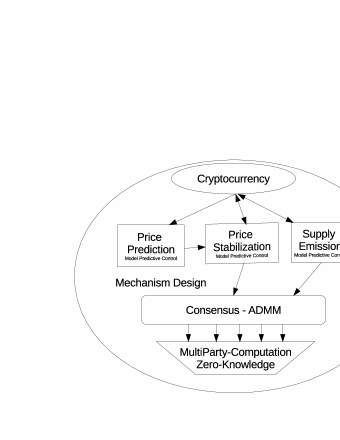
Figure 1: High-level rendering of the combination of techniques

4 Economic Models

We formalise a basic model of a cryptocurrency issuing variable block rewards and periodically auctioning a variable amount of unissued coins from its uncapped and dynamically adjusted supply: all these three variables are constantly adjusted by a dynamical system using Stochastic Model Predictive Control in order to maintain price stability (i.e., controlled variables).

Let $t\in T=\left\{1,\ldots,T\right\}$ denote the time slots used by the blockchain. Let $S_{max}(t)$ denote the maximum supply of a cryptocurrency, $S_{outstanding}(t)$ the supply that is visible on-chain, $S_{initial}$ the initially issued supply by an initial offering event (i.e., an initial auction) and $S_{unissued}(t)$ is the amount of cryptocurrency yet to be issued. Then, we have:

$$0 \leq S_{initial}\leq S_{outstanding}(t)\leq S_{max}(t),\forall t\in T,$$ (4.1)

$$S_{initial} = S_{outstanding}(1),$$ (4.2)

$$S_{max}(t) = S_{unissued}(t)+S_{outstanding}(t).$$ (4.3)

Periodically, miners are being rewarded for successfully processing blocks with a variable amount of block rewards, $BR(t)$:

$$S_{outstanding}(t+1) = S_{outstanding}(t)+BR(t),\forall t\in T,$$ (4.4)

$$S_{unissued}(t+1) = S_{unissued}(t)-BR(t),$$ (4.5)

$$0\leq BR(t)\leq BR_{max}.$$ (4.6)

Auctions are carried out to issue coins from the pool of $S_{unissued}(t)$ , each auction releasing a variable amount of auctioned coins, $AUC_{coins}(t)$, with $x_{i}(t)$ denoting the amount of coins demanded by participant $i$, $\forall t\in T$:

$$S_{outstanding}(t+1) = S_{outstanding}(t)+AUC_{coins}(t),$$ (4.7)

$$S_{unissued}(t+1) = S_{unissued}(t)-AUC_{coins}(t),$$ (4.8)

$$0\leq AUC_{coins}(t)\leq AUC_{max},$$ (4.9)

$$x_{i}^{min}(t)\leq x_{i}\left(t\right) \leq x_{i}^{max}\left(t\right),$$ (4.10)

$$\sum_{i}x_{i}(t) -AUC_{coins}(t) =0.$$ (4.11)

Let $P(t)$ denote the market price of a coin at time $t$ in a currency (i.e., the number of cryptocurrency coins that one unit of currency -EUR, JPY, USD- will buy at time $t$) and we adopt a geometric Brownian motion model:

$$\Delta P(t) = P(t+1)-P(t),$$ (4.12)

$$dP(t) = \mu P(t)dt+\sigma P(t)dW_{t},$$ (4.13)

where $W_{t}$ is a Weiner process. Let $\left\{S_{max}(t),BR(t),AUC_{coins}(t)\right\}$ be the controlled variables. Thus, in order to maintain price stability, these controlled variables will expand when the price is increasing and contract when the price is lowering:

$$S_{max}(t) \sim S_{max}(t-1)\cdot\frac{P(t)}{P(t-1)},$$ (4.14)

$$BR(t) \sim BR(t-1)\cdot\frac{P(t)}{P(t-1)},$$ (4.15)

$$AUC_{coins}(t) \sim AUC_{coins}(t-1)\cdot\frac{P(t)}{P(t-1)}.$$ (4.16)

4.1 Economic Model for an Algorithmic Stablecoin

Consider the stochastic linear state space system in the form

$$x_{k+1} = Ax_{k}+Bu_{k}+w_{k}$$ (4.17)

$$y_{k} = C_{y}x_{k}+v_{k}$$ (4.18)

$$z_{k} = C_{z}x_{k}$$ (4.19)

where $A,B,C_{y},C_{z}$ are state space matrices, $x_{k}\in\mathbb{R}^{n_{x}}$ is the state vector, $u_{k}\in\mathbb{R}^{n_{u}}$ is the input vector, $y_{k}\in\mathbb{R}^{n_{y}}$ is the output vector, $z_{k}\in\mathbb{R}^{n_{z}}$ is the vector of controlled variables, $w_{k}\in\mathbb{R}^{n_{x}}$ is the noise vector of the process, and $v_{k}\in\mathbb{R}^{n_{y}}$ is the vector of measurement noise. Let $N$ be the length of the prediction and receding horizon control and define the vectors

$$N_{i}=\left\{0+i,1+i,\ldots,N-1+i\right\}$$

$$u=\left[\begin{array}[]{cccc}u_{0}^{T}&u_{1}^{T}&\ldots&u_{N-1}^{T}\end{array}\right]^{T}, x=\left[\begin{array}[]{cccc}x_{1}^{T}&x_{2}^{T}&\ldots&x_{N}^{T}\end{array}\right]^{T},$$

$$z=\left[\begin{array}[]{cccc}z_{1}^{T}&z_{2}^{T}&\ldots&z_{N}^{T}\end{array}\right]^{T}, w=\left[\begin{array}[]{cccc}w_{1}^{T}&w_{2}^{T}&\ldots&w_{N}^{T}\end{array}\right]^{T}$$

Define the following exchange rate function measuring the cumulative exchange rate between the price of a currency (e.g., EUR, JPY, USD) and a stablecoin in the stochastic state space system 4.17 in the following $N$ time steps,

$$\begin{array}[]{c}\psi_{xch}\left(u;\bar{x}_{0},w\right)=\left\{\phi\left(u,x,z\right)\left|x_{0}=\bar{x}_{0},\right.\right.\\ \left.x_{k+1}=Ax_{k}+Bu_{k}+w_{k},z_{k+1}=Cx_{k+1},k\in N_{0}\right\},\end{array}$$ (4.22)

Let $P\left(t\right)$ be the spot price of the stablecoin cryptocurrency denominated in a currency (e.g., EUR, JPY, USD). Then, the cumulative exchange rate at time $t$ is

$$\phi\left(u,x,z\right)=\sum_{t=1}^{N}\left(P\left(t+1\right)\right)$$ (4.23)

Following a criterion of social welfare maximisation, users and holders of the stablecoin prefer to minimise the volatility of the exchange rate, with the following equation describing the minimisation problem

$$\underset{\forall t}{\mbox{minimise }}\lambda E\left[\psi_{xch}\right]+\left(1-\lambda\right)\mbox{Var}\left[\psi_{xch}\right]$$ (4.24)

with $\lambda\in\left[0,1\right]$ determines the trade-off between the expected exchange rate and the exchange rate variance.

4.2 Economic Model for a Collaterised Stablecoin

We extend the basic model of a cryptocurrency (4), with a reserve $R\left(t\right)$ backing every issued coin with $\lambda$ units of the reserve asset: for example, $\lambda=1$ for a 1 to 1 peg against a currency (e.g., EUR, JPY, USD), and $\lambda>1$ for an overcollaterised stablecoin backed with other cryptocurrencies. Then, we have:

$$R\left(t\right) = \lambda\cdot S_{outstanding}\left(t\right),$$ (4.25)

$$0\leq R\left(t\right) \leq\lambda\cdot S_{max}\left(t\right),$$ (4.26)

In order to maintain price stability, $\lambda\left(t\right)$ could also be a controlled variable that will increase when the price is lowering and contract when the price is increasing:

$$\lambda\left(t\right) \sim \lambda(t-1)\cdot\frac{P(t-1)}{P(t)},$$ (4.27)

$$1\leq \lambda\left(t\right) \leq\lambda_{max}.$$ (4.28)

4.3 Economic Model for a Central-Banked Currency

The framework and results of this paper could also be applied to the monetary policy conducted by central banks, just by representing their models in the framework of Model Predictive Control in a way similar to the previous Economic Model for an Algorithmic Stablecoin.

The Taylor rule[Tay93] is an approximation of the responsiveness of the nominal short-term interest rate $i_{t}$ as applied by the central bank to changes in inflation $\pi$ and output $y$, according to the following formula

$$i_{t}=\varphi_{y}\left(y_{t}-y^{*}\right)+\varphi_{\pi}\left(\pi_{t}-\pi^{*}\right)+\pi^{*}+r^{*}$$ (4.29)

where a standard model describes the evolution of the economy

$$\pi_{t+1} = \pi_{t}+\alpha y_{t}+e_{t+1}^{\pi},$$ (4.30)

$$y_{t+1} = \rho y_{t}-\zeta\left(i_{t}-\pi_{t}\right)+e_{t+1}^{y},$$ (4.31)

describing the dynamic relationship between the manipulated input $i_{t}$ and the two controlled outputs $y_{t}$ and $\pi_{t}$. At equilibrium, we obtain $i_{t}=i^{*}$, $\pi_{t}=\pi^{*}$, $y_{t}=0$ and $r^{*}=i^{*}-\pi^{*}$. Equations 4.30 and 4.31 can be rewritten in the terms of deviation variables from the equilibrium point, as

$$x_{t+1}=Ax_{t}+Bu_{t}+\epsilon_{t+1},$$ (4.32)

where

$$x = \left[\begin{array}[]{cc}y&-y^{*}\\ \pi&-\pi^{*}\end{array}\right],u=\Delta i=i-i^{*},\epsilon=\left[\begin{array}[]{c}e^{y}\\ e^{\pi}\end{array}\right],$$ (4.37)

$$A = \left[\begin{array}[]{cc}\rho&\zeta\\ \alpha&1\end{array}\right],$$ (4.40)

$$B = \left[\begin{array}[]{c}-\zeta\\ 0\end{array}\right]$$ (4.43)

The cost function of the central bank is of the standard optimal control form

$$\sum_{k=0}^{\alpha}\beta^{k}L\left(\hat{x}_{t+k\left|t\right.},u_{t+k\left|t\right.}\right)$$ (4.44)

where $\beta\in\left(0,1\right)$ is the discount factor, $\hat{x}_{t+k\left|t\right.}$ is the expected value of $x$ at time $t+x$ using all information available at time $t$ and model 4.32; $u_{t+k\left|t\right.}$ is the input value at time $t+k$ decided on at time $t$; and the $M$ function is usually defined as

$$M\left(\hat{x}_{t+k\left|t\right.},u_{t+k\left|t\right.}\right)=\hat{x}_{t+k\left|t\right.}^{T}Q\hat{x}_{t+k\left|t\right.}+R^{2}u_{t+k\left|t\right.}^{2}$$ (4.45)

with $R^{2}\geq 0$ and $Q\succeq 0$. The previous equations 4.44 and 4.45 can be reformulated as an objective for Model Predictive Control as

$$\underset{u}{\mbox{min}}\begin{array}[]{c}\left\{\sum_{k=0}^{N-1}\beta^{k}\left(\hat{x}_{t+k\left|t\right.}^{T}Q\hat{x}_{t+k\left|t\right.}+R^{2}u_{t+k\left|t\right.}^{2}+S^{2}\delta u_{t+k\left|t\right.}^{2}\right)\right.\\ \left.+\hat{x}_{t+N\left|t\right.}^{T}\beta^{N}\bar{Q}\hat{x}_{t+N\left|t\right.}+\beta^{N}S^{2}\delta u_{t+N\left|t\right.}^{2}\right\}\end{array}$$ (4.46)

where

$$Q = \left[\begin{array}[]{cc}1-\lambda&0\\ 0&\lambda\end{array}\right]\succ 0,0<\lambda<1,$$ (4.49)

$$u = \left[\Delta i_{t\left|t\right.}\ldots\Delta i_{t+N-1\left|t\right.}\right]^{T},$$ (4.50)

$$\delta u_{t+k\left|t\right.} = u_{t+k\left|t\right.}-u_{t+k-1\left|t\right.},k=0,\ldots,N$$ (4.51)

$$u_{t+k\left|t\right.} \geq -i^{*},k=0,\ldots,N-1,$$ (4.52)

$$u_{t+k\left|t\right.} = u_{t+m-1\left|t\right.},k=m,\ldots,N-1,$$ (4.53)

$$\hat{x}_{t+k\left|t\right.}^{T} = \sum_{l=0}^{k-1}A^{l}Bu_{t+k-l-1\left|t\right.}+A^{k}x_{t},k=1,\ldots,N$$ (4.54)

with $\hat{x}_{t\left|t\right.}=x_{t}$ and the values of $1-\lambda$ and $\lambda$ determine the trade-off between the output gap and inflation.

The decentralised implementation of the previous Model Predictive Control 4.46 using the ADMM decomposition technique is left as an exercise to the central banker.

4.3.1 Closed-Loop Stability

The following closed-loop structure is obtained from 4.29 and 4.32:

$$x_{t+1}=A^{{}^{\prime}}x_{t}+\epsilon_{t+1},$$ (4.55)

where

$$A^{{}^{\prime}}=A+Bc^{T}=\left[\begin{array}[]{cc}\rho-\zeta\varphi_{y}&\zeta-\zeta\varphi_{\pi}\\ \alpha&1\end{array}\right]$$ (4.56)

Theorem 1.

The Model Predictive Controller for the Taylor rule 4.46-4.54 has closed-loop stability, if and only if,

$$0.1\varphi_{\pi}-2.1 <\varphi_{y}$$ (4.57)

$$\varphi_{y}< 0.06\varphi_{\pi}+8.5,$$ (4.58)

$$\varphi_{\pi} > 1.$$ (4.59)

Proof.

The characteristic equation for the matrix $A^{{}^{\prime}}$ is:

$$f\left(\mu\right)=\mu^{2}-\mu\left(\alpha\zeta-\zeta\varphi_{y}-\alpha\zeta\varphi_{\pi}+1+\rho\right)+\left(\rho-\zeta\varphi_{y}\right)$$ (4.60)

where $\mu$ is an eigenvalue of matrix $A^{{}^{\prime}}$. The closed-loop system is stable when both eigenvalues of $A^{{}^{\prime}}$ are inside the unit disk (Jury[Jur74] and Routh[Rou77]-Hurtwiz[Hur95] stability criteria), if and only if,

$$2+2\rho-2\zeta\varphi_{y}+\alpha\zeta\left(\varphi_{\pi}-1\right) > 0,$$ (4.61)

$$1-\rho+\zeta\varphi_{y}-\alpha\zeta\left(\varphi_{\pi}-1\right) > 0,$$ (4.62)

$$\alpha\zeta\left(\varphi_{\pi}-1\right) > 0.$$ (4.63)

∎

Similar stability results can be derived for the Model Predictive Controllers of the Economic Model for an Algorithmic Stablecoin and the Economic Model for a Collaterised Stablecoin.

4.3.2 On Negative Interests

The Model Predictive Controller for the Taylor rule (4.46)-(4.54) includes a constraint for the zero lower bound on the interest rate, (LABEL:zero-lower-bound):

$$u_{t+k\left|t\right.}\geq-i^{*},k=0,\ldots,N-1.$$

In case the central bank wants to implement negative interest rates, said (LABEL:zero-lower-bound) must be removed. A possible implementation of negative interests for a cryptocurrency starts by considering coinage epochs and then defining a depreciation rate for every coinage epoch as time elapses. In the basic model of a cryptocurrency (4), we could add the following equation:

$$S_{outstanding}\left(t\right) = \sum_{t=0}^{T}\left(S_{minted}\left(t\right)-D_{T}\left(t\right)\right),$$ (4.64)

$$S_{initial} = S_{minted}(1)=S_{outstanding}(1),$$ (4.65)

$$0 \leq S_{initial}\leq S_{outstanding}(t)\leq S_{minted}\left(t\right)\leq S_{max}(t),\,\,\,\,\,\,\,$$ (4.66)

where $S_{minted}\left(t\right)$ is the amount of minted coins at time $t$ and $D_{T}\left(t\right)$ is the depreciation of coins minted at time $t$ evaluated at time $T$, for example,

$$D_{T}\left(t\right) = \mbox{min}\left(\left(T-t\right)\cdot D_{rate}\cdot S_{minted}\left(t\right),S_{minted}\left(t\right)\right),$$ (4.67)

$$D_{rate} = 0.01,$$ (4.68)

for a 1% depreciation rate for every coinage epoch since the first epoch.

5 Decentralised Prediction of Currency Prices through Deep Learning

As noted in previous publications about predicting markets using Stochastic Model Predictive Control techniques[PB17], this approach is only justifiable only for consistent prediction of the direction of price changes (i.e., sign changes): thus, it’s a requisite to use artificial intelligence techniques to predict price movements in order to maintain price stability. Of course, price data can be shifted by one sampling interval to the past, thereby making the economic models independent of any predictive power: however, the correct formulation is to use any potential good estimate of step-ahead prices as this is the core of Stochastic Model Predictive Control. Therefore, the exchange rate function 4.23 of the models is formulated with one step-ahead prices ($P\left(t+1\right)$).

A neural network has $L$ layers, each defined by a linear operator $W_{l}$ and a neural non-linear activation function $h_{l}$. A layer computes and outputs the non-linear function:

$$a_{l}=h_{l}\left(W_{l}a_{l-1}\right)$$ (5.1)

on input activations $a_{l-1}$. By nesting the layers, composite functions are obtained, for example,

$$f\left(a_{0},W\right)=W_{4}\left(h_{3}\left(W_{3}\left(h_{2}\left(W_{2}h_{1}\left(W_{1}a_{0}\right)\right)\right)\right)\right)$$ (5.2)

where the collection of weight matrices is $W=\left\{W_{l}\right\}$. Training a neural network for deep learning is the task of finding the $W$ that matches the output activations $a_{L}$ to targets $y$, given inputs $a_{0}$: it’s equivalent to the following minimisation problem, given loss function $l$,

$$\underset{W}{\mbox{minimise}}l\left(f\left(a_{0};W\right),y\right)$$ (5.3)

And this is equivalent to solving the following problem:

$$\underset{\left\{W_{l}\right\},\left\{a_{l}\right\},\left\{z_{l}\right\}}{\mbox{minimise}} l\left(z_{L},y\right)$$ (5.4)

subject to $$z_{l}= W_{l}a_{l-1},\mbox{ for }l=1,2,\ldots,L,$$ (5.5)

$$a_{l}= h_{l}\left(z_{l}\right),\mbox{ for }l=1,2,\ldots,L-1,$$ (5.6)

where a new variable stores the output of layer $l$, $z_{l}=W_{l}a_{l-1}$, and the output of the link function is represented as a vector of activations $a_{l}=h_{l}\left(z_{l}\right)$. By following the penalty method, a ridge penalty function is added to obtain the following unconstrained problem

$$\begin{array}[]{c}\underset{\left\{W_{l}\right\},\left\{a_{l}\right\},\left\{z_{l}\right\}}{\mbox{minimise}}\left\langle z_{L},\lambda\right\rangle+l\left(z_{L},y\right)+\beta_{L}\left\|z_{L}-W_{L}a_{L-1}\right\|^{2}\\ +\sum_{l=1}^{L-1}\left[\beta_{l}\left\|z_{l}-W_{l}a_{l-1}\right\|^{2}+\gamma_{l}\left\|a_{l}-h_{l}\left(z_{l}\right)\right\|^{2}\right]\end{array}$$ (5.7)

where $\left\{\gamma_{l}\right\}$ and $\left\{\beta_{l}\right\}$ are constants controlling the weight of each constraint, and $\left\langle z_{L},\lambda\right\rangle$ is a Lagrange multiplier term. The advantage of the previous formulation resides in that each sub-step has a simple closed-form solution with only one variable, thus these sub-problems can be solved globally.

The update steps of each variable in the minimisation problem 5.7 are considered as follows:

• To obtain $W_{l}$, each layer minimises $\left\|z_{l}-W_{l}a_{l-1}\right\|^{2}$: the solution of this least square problem is

  $$W_{l}\leftarrow z_{l}a_{l+1}^{+}$$ (5.8)

  where $a_{l+1}^{+}$ is the pseudo-inverse of $a_{l+1}$.

• To obtain $a_{l}$, another least-squares problem must be solved. The solution is

  $$a_{l}\leftarrow\left(\beta_{l+1}W_{l+1}^{T}W_{l+1}+\gamma_{l}I\right)^{-1}\left(\beta_{l+1}W_{l+1}^{T}z_{l+1}+\gamma_{l}h_{l}\left(z_{l}\right)\right)$$ (5.9)

• The update for $z_{l}$ requires minimising

  $$\mbox{arg min}_{z}\gamma_{l}\left\|a_{l}-h_{l}\left(z\right)\right\|^{2}+\beta_{l}\left\|z_{l}-W_{l}a_{l-1}\right\|^{2}$$

• Finally, the update of the Lagrange multiplier is given by

  $$\lambda\leftarrow\lambda+\beta_{L}\left(z_{L}-W_{L}a_{L-1}\right)$$ (5.10)

All the previous steps are listed in the next Algorithm 1:

do   for $l=1,2,\ldots,L-1$ do     $W_{l}\leftarrow z_{l}a_{l+1}^{+}$     $a_{l}\leftarrow\left(\beta_{l+1}W_{l+1}^{T}W_{l+1}+\gamma_{l}I\right)^{-1}\left(\beta_{l+1}W_{l+1}^{T}z_{l+1}+\gamma_{l}h_{l}\left(z_{l}\right)\right)$     $z_{l}\leftarrow\mbox{arg min}_{z}\left(\gamma_{l}\left\|a_{l}-h_{l}\left(z\right)\right\|^{2}+\beta_{l}\left\|z_{l}-W_{l}a_{l-1}\right\|^{2}\right)$   end for   $W_{L}\leftarrow z_{L}a_{L-1}^{+}$   $z_{l}\leftarrow\mbox{arg min}_{z}\left(l\left(z,y\right)+\left\langle z_{L},\lambda\right\rangle+\beta_{L}\left\|z-W_{L}a_{l-1}\right\|^{2}\right)$   $\lambda\leftarrow\lambda+\beta_{L}\left(z_{L}-W_{L}a_{L-1}\right)$ until converged; Algorithm 1 ADMM algorithm for Deep Learning

Finally, note that more advanced methods for training neural networks for deep learning have appeared in the literature[XWZ⁺19, WYCZ19], also considering their convergence.

6 Decentralised Stabilisation of Stablecoins

Following the Economic Model for an Algorithmic Stablecoin and its minimisation problem (4.24), the expectation of the exchange rate and the variance of the exchange rate are traded off in a mean-variance Optimal Control Problem with the following objective function

$$\psi=\lambda E_{w}\left[\psi_{xch}\right]+\left(1-\lambda\right)\mbox{Var}_{w}\left[\psi_{xch}\right]$$ (6.1)

with $\lambda\in\left[0,1\right]$ determining the trade-off between the expected exchange rate and the exchange rate variance. Estimates of prices for the expected exchange rate, $E_{w}\left[\psi_{xch}\right]$, and the variance, $\mbox{Var}_{w}\left[\psi_{xch}\right]$, are introduced as follows

$$E_{w}\left[\psi_{xch}\right] \approx \mu=\frac{1}{S}\sum_{i\in S}\psi_{xch}\left(u;\hat{x}_{0},w^{i}\right)$$ (6.2)

$$\mbox{Var}_{w}\left[\psi_{xch}\right] \approx s^{2}=\frac{1}{S-1}\sum_{i\in S}\left(\psi_{xch}\left(u;\hat{x}_{0},w^{i}\right)-\mu\right)^{2}$$ (6.3)

where $w^{i}$ is sampled from the distribution $w$ and $S$ is the set of scenarios: when the number of scenarios is large, then

$$\psi\approx\tilde{\psi}=\lambda\mu+\left(1-\lambda\right)s^{2}$$ (6.4)

The open-loop input trajectory is defined as the trajectory, $u^{*}\in U$, that minimises (6.4), with $U$ being some input constraint set. For the stochastic linear system (4.17), $u^{*}$ can be expressed as the solution to the following Optimal Control Problem,

$$\underset{\left\{u^{j}\in U,x^{j},z^{j},\psi^{j}\right\}_{j=1}^{S},\mu}{\mbox{minimise}} \lambda\mu+\tilde{\lambda}\sum_{j\in S}\left(\psi^{j}-\mu\right)^{2}$$ (6.5)

subject to $$\left(x^{i},u^{i},z^{i}\right)\in H\left(\hat{x_{0}},w^{i}\right), i\in S,$$ (6.6)

$$\psi^{i}\geq\phi\left(u^{i},x^{i},z^{i}\right), i\in S,$$ (6.7)

$$\mu=\frac{1}{S}\sum_{j\in S}\psi^{j},$$ (6.8)

$$u_{k}^{i}=u_{k}^{j}, i,j\in S,j\in M$$ (6.9)

where $$\tilde{\lambda}=\frac{1-\lambda}{S-1},$$

$$M=\left\{0,1,\ldots,M\right\},$$

$$M\leq N,$$

$$H\left(\hat{x}_{0},w\right)=\left\{\left(x,z,u\right)\left|x_{0}=\hat{x}_{0},\right.\right.$$

$$x_{k+1}=Ax_{k}+Bu_{k}+w_{k},$$

$$\left.z_{k+1}=C_{z}x_{k+1},k\in N_{0}\right\}$$

The previous Optimal Control Problem (6.5) is a convex optimisation problem when $U$ is a convex set and $\phi$ is a convex function: an ADMM-based decomposition algorithm for (6.5) is presented below.

6.1 ADMM Decomposition

The Optimal Control Problem (6.5) is re-written as

$$\underset{u\in\tilde{U},x,z,\psi,\mu}{\mbox{minimise}} \lambda\mu+\tilde{\lambda}\psi^{T}\psi+S\tilde{\lambda}\mu^{2}-2\tilde{\lambda}\mu\mathbf{1}^{T}\psi,$$ (6.10)

subject to $$\tilde{A}x+\tilde{B}u+\tilde{w}=0,$$ (6.11)

$$z=\tilde{C}x,$$ (6.12)

$$\psi\geq\tilde{\phi}\left(u,x,z\right),$$ (6.13)

$$\mu=\mathbf{1}^{T}\psi/S,$$ (6.14)

$$\tilde{L}u=0,$$ (6.15)

where

$$u=\left[\begin{array}[]{c}u^{1}\\ u^{2}\\ \vdots\\ u^{S}\end{array}\right],x=\left[\begin{array}[]{c}x^{1}\\ x^{2}\\ \vdots\\ x^{S}\end{array}\right],z=\left[\begin{array}[]{c}z^{1}\\ z^{2}\\ \vdots\\ z^{S}\end{array}\right],\psi=\left[\begin{array}[]{c}\psi^{1}\\ \psi^{2}\\ \vdots\\ \psi^{S}\end{array}\right],$$

$$\mathbf{1}=\left[\begin{array}[]{cccc}1&1&\ldots&1\end{array}\right],$$

$$\tilde{A}=\mbox{{blkdiag}}\left(\bar{A},\bar{A},\ldots,\bar{A}\right), \tilde{B}=\mbox{{blkdiag}}\left(\bar{B},\bar{B},\ldots,\bar{B}\right), \tilde{C}=\mbox{{blkdiag}}\left(\bar{C},\bar{C},\ldots,\bar{C}\right),$$

$$\bar{B}=\mbox{{blkdiag}}\left(B,B,\ldots,B\right), \bar{C}=\mbox{{blkdiag}}\left(C,C,\ldots,C\right),$$

$$\bar{A}=\left[\begin{array}[]{cccc}-I\\ A&-I\\ &\ddots&\ddots\\ &&A&-I\end{array}\right],\bar{w}^{i}=\left[\begin{array}[]{c}w_{0}^{i}\\ w_{1}^{i}\\ \vdots\\ w_{N-1}^{i}\end{array}\right]+\left[\begin{array}[]{c}Ax_{0}\\ 0\\ \vdots\\ 0\end{array}\right],i\in S,$$

$$\tilde{w}=\left[\left(\bar{w}^{1}\right)^{T}\left(\bar{w}^{2}\right)^{T}\ldots\left(\bar{w}^{S}\right)^{T}\right]^{T},$$

$$\tilde{\phi}\left(u,x,z\right)=\left[\phi\left(u^{1},x^{1},z^{2}\right)\ldots\phi\left(u^{S},x^{S},z^{S}\right)\right]^{T},$$

$$\tilde{L}=\left[\begin{array}[]{ccccc}L&-L\\ &L&-L\\ &&\ddots&\ddots\\ &&&L&-L\end{array}\right],$$

$$L=\left[\begin{array}[]{cc}I&0\end{array}\right],$$

$$Lu^{i}=\left[\left(u_{1}^{i}\right)^{T}\left(u_{2}^{i}\right)^{T}\ldots\left(u_{M}^{i}\right)^{T}\right]^{T}$$

The previous Optimal Control Problem (6.10) is then transformed into ADMM form,

$$\underset{y_{1,}y_{2}}{\mbox{minimise}} f_{1}\left(y_{1}\right)+f_{2}\left(y_{2}\right),$$ (6.18)

subject to $$M_{1}y_{1}+M_{2}y_{2}=0,$$ (6.19)

with the optimisation variables defined as

$$y_{1} = \left[\begin{array}[]{ccccc}\check{u}^{T}&x^{T}&z^{T}&\check{\psi}^{T}&\check{\mu}\end{array}\right]^{T},$$ (6.21)

$$y_{2} = \left[\begin{array}[]{ccc}u^{T}&\psi^{T}&\mu^{T}\end{array}\right]^{T}$$ (6.23)

where

$$g=\left[\begin{array}[]{ccccc}0&0&0&0&\lambda\end{array}\right]^{T}, H=\left[\begin{array}[]{ccc}0&0&0\\ 0&\tilde{\lambda}I&-\tilde{\lambda}\mathbf{1}^{T}\\ 0&-\tilde{\lambda}\mathbf{1}&S\tilde{\lambda}\end{array}\right],$$ (6.28)

$$M_{1}=\left[\begin{array}[]{ccccc}0&0&0&0&1\\ 0&0&0&0&1\\ I&0&0&0&0\\ 0&0&0&I&0\end{array}\right], M_{2}=\left[\begin{array}[]{ccc}0&\frac{-\mathbf{1}^{T}}{S}&0\\ 0&0&-1\\ -I&0&0\\ 0&-I&0\end{array}\right],$$ (6.37)

$$f_{1}\left(y_{1}\right) = g^{T}y_{1}+I_{\mathbb{Y}_{1}}\left(y_{1}\right),$$ (6.38)

$$f_{2}\left(y_{2}\right) = y_{2}^{T}Hy_{2}+I_{\mathbb{Y}_{2}}\left(y_{2}\right),$$ (6.39)

$$\mathbb{Y}_{1} = \left\{y_{1}\mid\tilde{A}x+\tilde{B}\check{u}+\tilde{w}=0,z=\tilde{C}x,\check{\psi}\geq\tilde{\phi}\left(\check{u},x,z\right)\right\},$$ (6.40)

$$\mathbb{Y}_{2} = \left\{y_{2}\mid\tilde{L}u=0\right\}$$ (6.41)

6.2 Decentralised Iterated Computation

The Lagrangian of (6.18) and (6.19) is

$$\mathscr{L}\left(y_{1},y_{2},\zeta\right)=f_{1}\left(y_{1}\right)+f_{2}\left(y_{2}\right)+\zeta^{T}\left(M_{1}y_{1}+M_{2}y_{2}\right)$$ (6.42)

where $\zeta$ is a vector of Lagrangian multipliers for (6.19). In ADMM, points satisfying the optimality conditions for (6.18) and (6.19) are obtained via the recursions with iteration number $j$

$$\begin{array}[]{c}y_{1}\left(j+1\right)=\underset{y_{1}}{\mbox{arg min}}\mathscr{L}_{\rho}\left(y_{1},y_{2}\left(j\right),\zeta\left(j\right)\right)\\ =\underset{y_{1}}{\mbox{arg min}}f_{1}\left(y_{1}\right)+\frac{\rho}{2}\left\|M_{1}y_{1}+M_{2}y_{2}\left(j\right)+\eta\left(j\right)\right\|_{2}^{2}\end{array}$$ (6.45)

$$\begin{array}[]{c}y_{2}\left(j+1\right)=\underset{y_{2}}{\mbox{arg min}}\mathscr{L}_{\rho}\left(y_{1}\left(j+1\right),y_{2},\zeta\left(j\right)\right)\\ =\underset{y_{2}}{\mbox{arg min}}f_{2}\left(y_{2}\right)+\frac{\rho}{2}\left\|M_{1}y_{1}\left(j+1\right)+M_{2}y_{2}+\eta\left(j\right)\right\|_{2}^{2},\end{array}$$ (6.48)

$$\eta\left(j+1\right)=\eta\left(j\right)+\left(M_{1}y_{1}\left(j+1\right)+M_{2}y_{2}\left(j+1\right)\right)$$ (6.49)

where the augmented Lagrangian with penalty parameter $\rho>0$ is defined as

$$\mathscr{L}_{\rho}\left(y_{1},y_{2},\zeta\right)=\mathscr{L}\left(y_{1},y_{2},\zeta\right)+\frac{\rho}{2}\left\|M_{1}y_{1}+M_{2}y_{2}\right\|_{2}^{2}$$

and $\eta=\zeta/\rho$ is a scaled dual variable.

Stopping criteria for the previous recursions (6.45), (6.48) and (6.49) is given by

$$\left\|M_{1}y_{1}\left(j\right)+M_{2}y_{2}\left(j\right)\right\|_{2} \leq \varepsilon_{P},$$ (6.50)

$$\rho\left\|M_{1}^{T}M_{2}\left(y_{2}\left(j+1\right)-y_{2}\left(j\right)\right)\right\|_{2} \leq \varepsilon_{D},$$ (6.51)

indicating that the algorithm should be stopped when the optimality conditions for (6.18) and (6.19) are satisfied with accuracy as defined by the small tolerance levels $\varepsilon_{P}$ and $\varepsilon_{D}$.

The following Algorithm 2 describes the steps of the implementation of the ADMM recursions (6.45)-(6.49): further optimisations are possible to parallelise the algorithm in $S$.

while not converged do   // ADMM update of $y_{1}=\left(\begin{array}[]{ccccc}\check{u}^{T},&x^{T},&z^{T},&\check{\psi}^{T},&\check{\mu}\end{array}\right)$   $\left(\begin{array}[]{ccccc}\check{u}^{T},&x^{T},&z^{T},&\check{\psi}^{T},&\check{\mu}\end{array}\right)\leftarrow$compute via 6.45   // ADMM update of $y_{2}=\left(\begin{array}[]{ccc}u^{T},&\psi^{T},&\mu^{T}\end{array}\right)$   $\left(\begin{array}[]{ccc}u^{T}&\psi^{T}&\mu^{T}\end{array}\right)\leftarrow$compute via 6.48   // ADMM update of $\eta$   $\eta\leftarrow$compute via 6.49 end while Algorithm 2 ADMM algorithm for the Optimal Control Problem 6.5-6.9

Theorem 2.

The proposed decentralised mechanism in Algorithm 2 is a faithful decentralised implementation.

Proof.

The steps that every rational user $i$ will faithfully complete are the variable update steps of (6.45)-(6.49) in Algorithm 2.

Under the assumption of rational players in an ex-post Nash equilibrium (11), users can maximise their own utility only by maximising the social welfare (5). Therefore, every user will faithfully execute the variable update steps of (6.45)-(6.49) since it’s the only way to maximise social welfare when all the other rational users are following the intended strategy. ∎

7 Auction Mechanism for Issuing Stablecoins

At the beginning of an auction, each user reports its demand to the auction manager. We define the demand of user $i$ as

$$\theta_{i}=\left\{x_{i}^{min}\left(t\right),x_{i}\left(t\right),x_{i}^{max}\left(t\right)\right\}$$ (7.1)

Users can misreport their demands: let $\hat{\theta}_{i}=\left\{\hat{x}_{i}^{min}\left(t\right),\hat{x}_{i}\left(t\right),\hat{x}_{i}^{max}\left(t\right)\right\}$ denote the reported demand of user $i$. The auction manager determines the outcome of the auction including stablecoin allocation and payments according to the stablecoin allocation rule, $al\left(\right)$.

Denote the following variable definitions

$$x_{i}=\left[x_{i,1},\ldots,x_{i,T}\right], y=\left[y_{1},\ldots,y_{T}\right],$$

$$v_{i}\left(x_{i}\right)=\sum_{t\in T}v_{i,t}\left(x_{i,t}\right), c\left(y\right)=\sum_{t\in T}c_{t}\left(y_{t}\right).$$

where $v_{i,t}\left(x_{i,t}\right)$ is a concave function for the valuation of user $i$ at time $t$ and $c_{t}\left(y_{t}\right)$ is an always-positive convex function for the cost of the auction manager at time $t$ (i.e., this cost is the market value of the auctioned coins, plus other expenditures for carrying out the auction). The utility of user $i$ is defined as the valuation minus the payment

$$u_{i}\left(al\left(\hat{\theta}\right),\theta_{i}\right)=\sum_{t\in T}v_{i,t}\left(x_{i},t\right)-\sum_{t\in T}p_{i,t}\left(\hat{\theta}\right),$$ (7.2)

and the utility of the auction manager is the total payment minus the total cost,

$$\sum_{i\in N}\sum_{i\in T}p_{i,t}\left(\hat{\theta}\right)-\sum_{t\in T}c_{t}\left(y_{t}\right)$$ (7.3)

The stablecoin allocation rule of the auction mechanism is defined by the following social welfare maximisation problem

$$\mathscr{S}: \underset{x,y}{\mbox{maximise}}\sum_{i\in N}v_{i}\left(x_{i}\right)-c\left(y\right),$$ (7.4)

such that $$x_{i}\in X_{i}, \forall i\in N,$$ (7.5)

$$y\in Y,$$ (7.6)

$$\sum_{i\in N}A_{i}x_{i}+By=0,$$ (7.7)

where $X_{i}$ is the constraint set of user $i$ for satisfying (4.10) $\forall t\in T$; $Y$ is the constraint set of the blockchain satisfying (4.1)-(4.9) and (4.12)-(4.16) $\forall t\in T$; $A_{i}$ and $B_{i}$ are the constraint set for satisfying (4.11) $\forall t\in T$ equivalent to constraint (7.7).

The optimal solution to the social welfare maximisation problem $\mathscr{S}$ is denoted by $\left\{x^{*},y^{*}\right\}$, in which $x^{*}$ is the outcome of stablecoin allocation to users whenever all users truthfully report their demands to the auction mechanism.

The payment by user $i$ at time slot $t$ is defined as the following equation according to the VCG payment rule[NR07, PS04],

$$p_{i,t}\left(\theta\right)=\sum_{j\neq i}v_{j,t}\left(x_{j,t}^{-i}\right)-\sum_{j\neq i}v_{j,t}\left(x_{j,t}^{*}\right)+c_{t}\left(y_{t}^{*}\right),$$ (7.8)

where $x^{-i}=\left\{x_{j,t}^{-i}\left|j\in N\setminus\left\{i\right\},t\in T\right.\right\}$: at the same time, the payment by user $i$ at time slot $t$ is the optimal solution to the following maximisation problem that excludes user $i$,

$$\mathscr{S}_{-i}: \underset{x}{\mbox{maximise}}\sum_{j\neq i}v_{j}\left(x_{j}\right),$$ (7.9)

such that $$x_{j}\in X_{j}, \forall j\in N\setminus\left\{i\right\}$$ (7.10)

7.1 Properties of the Auction Mechanism

In the proposed auction mechanism, each user achieves maximum utility only when said user truthfully reports its demand $\theta_{i}$: a mechanism is incentive-compatible if truth-revelation by users is obtained in an equilibrium[NR07, PS04].

Let $s_{i}\left(\theta_{i}\right)$ denote the strategy of user $i$ given $\theta_{i}$ and let

$$\theta_{-i}=\left\{\theta_{1},\ldots,\theta_{i-1},\theta_{i+1},\ldots,\theta_{N}\right\}$$

Definition 3.

(Dominant-Strategy Equilibrium[SPS03]). A strategy profile $s^{*}$ is a dominant-strategy equilibrium of a game if, for all $i$,

$$u_{i}\left(f\left(s_{i}^{*}\left(\theta_{i}\right),s_{-i}\left(\theta_{-i}\right)\right),\theta_{i}\right)\geq u_{i}\left(f\left(s_{i}\left(\theta_{i}\right),s_{-i}\left(\theta_{-i}\right)\right),\theta_{i}\right)$$ (7.11)

holds $s_{i}\left(\theta_{i}\right)\in\varTheta_{i}$, $\forall\theta_{i}$, $\forall\theta_{-i}$ and $\forall s_{i}\neq s_{i}^{*}$.

Definition 4.

(Strategy-Proof Mechanism[SPS03]). A mechanism is strategy-proof if truthfully reporting demand $\theta_{i}$ is the best strategy of user $i$, no matter what the other users report: that is, the incentive-compatibility of a mechanism in a dominant-strategy equilibrium is only achieved when the following condition holds

$$u_{i}\left(f\left(\theta_{i},\hat{\theta}_{-i}\right),\theta_{i}\right)\geq u_{i}\left(f\left(\hat{\theta}_{i},\hat{\theta}_{-i}\right),\theta_{i}\right)$$ (7.12)

The proposed auction mechanism is incentive-compatible and strategy-proof in a dominant-strategy equilibrium.

Theorem 5.

The proposed auction mechanism (7.4)-(7.7) and (7.8) is strategy-proof.

Proof.

We prove that each user will truthfully report their demand in order to show that the auction mechanism is strategy-proof.

For their demanded amount $x_{i}(t)$, the payment rule (7.8) was designed according to the VCG payment rule[NR07, PS04] so that user’s utility is maximised only when it truthfully reports its demand.

For the lower bound $x_{i}^{min}\left(t\right)$, user $i$ will not understate $x_{i}^{min}\left(t\right)$ to ensure that the minimum demanded is satisfied. A user will not overstate $x_{i}^{min}\left(t\right)$ to avoid limiting the growth of the social welfare: to understand the underlying reason, we write the utility of the user with the payment rule expanded

$$u_{i}\left(al\left(\hat{\theta}\right),\theta_{i}\right)=v_{i}\left(x_{i}^{*}\right)-\sum_{j\neq i}v_{j}\left(x_{j}^{-i}\right)+\sum_{j\neq i}v_{j}\left(x_{j}^{*}\right)-c\left(y^{*}\right),$$

and note that a user cannot influence the second term by misreporting their demand $\hat{\theta}$. A user maximising utility can only maximise the other terms (i.e., social welfare). Therefore, user $i$ will not overstate $x_{i}^{min}\left(t\right)$.

For the upper bound $x_{i}^{max}\left(t\right)$, for similar reasons to the previous $x_{i}^{min}\left(t\right)$, understating $x_{i}^{max}\left(t\right)$ would only limit the growth of the social welfare, thus user $i$ is not incentivised to understate $x_{i}^{max}\left(t\right)$. On the other side, overstating $x_{i}^{max}\left(t\right)$ would lead to a larger stablecoin allocation than the real user’s demand: the auction manager would detect such a situation when later the user is unable to pay the overstated allocation, and penalises the user with much higher prices for a much lower amount of coins. Thus, user $i$ will not overstate $x_{i}^{max}\left(t\right)$ in order to prevent penalties.∎

Theorem 6.

The proposed auction is budget-balanced, that is, the received payment is no less than the total cost.

Proof.

The total payment that the auction manager receives is

$$\sum_{i\in N}\sum_{i\in T}p_{i,t}\left(\theta\right)=\sum_{i\in N}\sum_{j\neq i}v_{j}\left(x_{j}^{-i}\right)-\sum_{i\in N}\sum_{j\neq i}v_{j}\left(x_{j}^{*}\right)+N\cdot c\left(y^{*}\right)$$

Note that

$$\sum_{j\neq i}v_{j}\left(x_{j}^{-i}\right)\geq\sum_{j\neq i}v_{j}\left(x_{j}^{*}\right)$$

because $x^{-i}$ is the optimal solution to (7.9) and that, by definition, $c\left(y^{*}\right)\geq 0$. Therefore, we conclude

$$\sum_{i\in N}\sum_{i\in T}p_{i,t}\left(\theta\right)\geq N\cdot c\left(y^{*}\right)\geq c\left(y^{*}\right).$$

∎

8 Decentralised Implementation of Auction Mechanism

A decentralised implementation of the centralised auction mechanism (7.4) is achieved in this section: proximal dual consensus ADMM[BPC⁺11, Cha14] is used to solve problem $\mathscr{S}$.

8.1 Dual Consensus ADMM

We start adding a polyhedra constraint to the stablecoin allocation rule (7.4)-(7.7):

$$\mathscr{S}: \underset{x,y}{\mbox{maximise}}\sum_{i\in N}v_{i}\left(x_{i}\right)-c\left(y\right),$$ (8.1)

such that $$x_{i}\in X_{i}, \forall i\in N,$$ (8.2)

$$y\in Y,$$ (8.3)

$$\sum_{i\in N}A_{i}x_{i}+By=0,$$ (8.4)

$$C_{i}x_{i}\preceq d_{i}, i=1,\ldots,N,$$ (8.5)

where each $x_{i}$ in (8.5) is a local constraint set of user $i$ consisting of simple polyhedra constraint $C_{i}x_{i}\preceq d_{i}$, such that there would be closed-form solutions to efficiently solve all the subproblems at every iteration.

Let $\lambda$ be the dual variable of constraint (8.4), and $z_{i}$ be the dual variable of (8.5): the Lagrange dual problem of $\mathscr{S}$, equivalent to solving problem $\mathscr{S}$ since it’s a concave maximisation problem, is defined by

$$\underset{\lambda,z_{i}}{\mbox{minimise}}\sum_{i\in N}\phi_{i}\left(\lambda,z_{i}\right)+z_{i}^{T}d_{i}+\psi\left(\lambda\right),$$ (8.6)

where

$$\phi_{i}\left(\lambda,z_{i}\right) = \underset{x_{i}\in X_{i}}{\mbox{maximise}}\left\{v_{i}\left(x_{i}\right)-\lambda^{T}A_{i}x_{i}-z_{i}^{T}\left(C_{i}x_{i}+r_{i}\right)\right\},\forall i\in N,$$ (8.7)

$$\psi\left(\lambda\right) = \underset{y\in Y}{\mbox{maximise}}\left\{-c\left(y\right)-\lambda^{T}By\right\}$$ (8.8)

where $r_{i}$ are slack variables. Let’s obtain a copy of $\lambda$ for every user $i$, denoted by $\lambda_{i}$, by rewriting the previous problem into the following equivalent problem,

$$\underset{\lambda,z_{i},\left\{\lambda_{i}\right\},\left\{\lambda_{i}^{{}^{\prime}}\right\}}{\mbox{minimise}}\sum_{i\in N}\phi_{i}\left(\lambda_{i},z_{i}\right)+z_{i}^{T}d_{i}+\psi\left(\lambda\right)$$ (8.9)

such that $$\lambda_{i}=\lambda_{i}^{{}^{\prime}}, \forall i\in N,$$ (8.10)

$$\lambda=\lambda_{i}^{{}^{\prime}},$$ (8.11)

In blockchain settings, there could be some users offline and/or some communication links could be interrupted: at each iteration, each user $i$ has probability $\alpha_{i}\in\left(0,1\right]$ of being online, and each link $\left(i,j\right)$ has probability $p_{e}\in\left(0,1\right]$ of being interrupted; the probability that user $i$ and user $j$ are both active and able to exchange messages is given by $\beta_{ij}=\alpha_{i}\alpha_{j}\left(1-p_{e}\right)$. For each iteration $k$, let $\Omega^{k}$ be the set of active users and $\Psi^{k}\subseteq\left\{\left(i,j\right)|i,j\in\Omega^{k}\right\}$ be the set of active edges.

The variable update steps of the auction manager at iteration $k$ are given by the following equations:

$$\mu^{\left[k\right]}=\mu^{\left[k-1\right]}+q\sum_{i\in N}\left(\lambda^{\left[k-1\right]}-\lambda_{i}^{\left[k-1\right]}\right),$$ (8.12)

$$\begin{array}[]{c}y^{\left[k\right]}=\underset{y\in Y}{\mbox{arg min}}\left\{c\left(y\right)+\frac{q}{4N}\left\|\frac{1}{q}By-\frac{1}{q}\mu^{\left[k\right]}\right.\right.\\ \left.+\sum_{i\in N}\left(\lambda^{\left[k-1\right]}+\lambda_{i}^{\left[k-1\right]}\right)\parallel_{2}^{2}\right\},\end{array}$$ (8.15)

$$\lambda^{\left[k\right]}=\frac{1}{2N}\left(\frac{1}{q}By^{\left[k\right]}-\frac{1}{q}\mu^{\left[k\right]}+\sum_{i\in N}\left(\lambda^{\left[k-1\right]}+\lambda_{i}^{\left[k-1\right]}\right)\right)$$ (8.16)

with $\mu$ represents the dual variables $\lambda_{i}=\lambda_{i}^{{}^{\prime}}$ and $q$ is a positive constant. The variable update steps of user $i$ at iteration $k$ are given by the following equations:

$$\forall i\in\Omega^{k}:$$ (8.29)

$$\mu_{i}^{\left[k\right]}=\mu_{i}^{\left[k-1\right]}+2q\left(\lambda_{i}^{\left[k-1\right]}-t_{ij}^{\left[k-1\right]}\right),$$

$$\begin{array}[]{c}\left(x_{i}^{\left[k\right]},r_{i}^{\left[k\right]}\right)=\underset{x_{i}\in X_{i},r_{i}\succ 0}{\mbox{arg min}}\left\{-v_{i}\left(x_{i}\right)+\frac{q}{4}\left\|\frac{1}{q}A_{i}x_{i}-\frac{1}{q}\mu_{i}^{\left[k\right]}\right.\right.\\ +2t_{ij}^{\left[k-1\right]}\parallel_{2}^{2}\\ \left.+\frac{1}{2\sigma_{i}}\left\|C_{i}x_{i}+r_{i}-d_{i}+\sigma_{i}z_{i}^{k-1}\right\|_{2}^{2}\right\},\end{array}$$

$$z_{i}^{\left[k\right]}=z_{i}^{\left[k-1\right]}+\frac{1}{\sigma_{i}}\left(C_{i}x_{i}^{\left[k\right]}+r_{i}^{\left[k\right]}-d_{i}\right),$$

$$t_{ij}^{\left[k\right]}=\left\{\begin{array}[]{cc}\frac{\lambda_{i}^{\left[k\right]}+\lambda_{j}^{\left[k\right]}}{2},&\mbox{if }\left(i,j\right)\in\Psi^{k},\\ t_{ij}^{\left[k-1\right]},&\mbox{otherwise},\end{array}\right.$$

$$\lambda_{i}^{\left[k\right]}=\frac{1}{2q}A_{i}x_{i}^{\left[k\right]}-\frac{1}{2q}\mu_{i}^{\left[k\right]}+t_{ij}^{\left[k-1\right]},$$

$$\forall i\notin\Omega^{k}:$$

$$\begin{array}[]{c}x_{i}^{\left[k\right]}\neq x_{i}^{\left[k-1\right]},r_{i}^{\left[k\right]}\neq r_{i}^{\left[k-1\right]},\lambda_{i}^{\left[k\right]}\neq\lambda_{i}^{\left[k-1\right]},z_{i}^{\left[k\right]}\neq z_{i}^{\left[k-1\right]},\\ \mu_{i}^{\left[k\right]}\neq\mu_{i}^{\left[k-1\right]},t_{ij}^{\left[k\right]}\neq t_{ij}^{\left[k-1\right]}\forall j\in N_{i},\end{array}$$

where $\sigma_{i}$ are penalty parameters. The following stopping criteria for the success of the convergence are applied by the auction manager

$$\left\|\lambda^{\left[k\right]}-\bar{\lambda}^{\left[k\right]}\right\|_{2}^{2}+\sum_{i\in N}\left\|\lambda_{i}^{\left[k\right]}-\bar{\lambda}^{\left[k\right]}\right\|_{2}^{2}\leq\varepsilon_{1},$$ (8.30)

$$\left\|\bar{\lambda}^{\left[k\right]}-\bar{\lambda}^{\left[k-1\right]}\right\|_{2}^{2}\leq\varepsilon_{2},$$ (8.31)

where $\varepsilon_{1}$ and $\varepsilon_{2}$ are small positive constants and

$$\bar{\lambda}^{\left[k\right]}=\left(\lambda^{\left[k\right]}+\sum_{i\in N}\lambda_{i}^{\left[k\right]}\right)/\left(N+1\right)$$

The following Algorithm 3 shows the dual consensus ADMM for problem $\mathscr{S}$:

$k=0$ Auction manager only: $\mu^{\left[0\right]}=0$, $y^{\left[0\right]}\in\mathbb{R}^{15T},\lambda^{\left[0\right]}\in\mathbb{R}^{3T}$ User $i$ only: $\mu_{i}^{\left[0\right]}=0$, $x_{i}^{\left[0\right]}\in\mathbb{R}^{15T},r_{i}^{\left[0\right]}\in\mathbb{R}^{15T},z_{i}^{\left[0\right]}\in\mathbb{R}^{15T},\lambda_{i}^{\left[0\right]}\in\mathbb{R}^{3T}$ and $$t_{ij}^{\left[0\right]}=\frac{\lambda_{i}^{0}+\lambda_{j}^{0}}{2}$$ repeat   $k\leftarrow k+1$   Auction manager only: send $\lambda^{\left[k-1\right]}$ to every user $i$   Auction manager only: update $\mu^{\left[k\right]},y^{\left[k\right]}$ and $\lambda^{\left[k\right]}$ according to (8.12)-(8.16)   for parallel $i\in N$ do     User $i$ only: send $\lambda_{i}^{\left[k-1\right]}$ to auction manager     User $i$ only: update $\mu_{i}^{\left[k\right]},x_{i}^{\left[k\right]}$, $r_{i}^{\left[k\right]}$, $z_{i}^{\left[k\right]}$, $t_{ij}^{\left[k\right]}$ and $\lambda_{i}^{\left[k\right]}$ according to (8.29)-(8.29)   end for until convergence is achieved by stopping criteria (8.30) and (8.31); Algorithm 3 Dual Consensus ADMM for Problem $\mathscr{S}$

Theorem 7.

Algorithm 3 converges to the optimal solution of problem $\mathscr{S}$ in the mean, with a $O\left(1/k\right)$ worst-case convergence rate.

Proof.

Follows from Theorem 2 from [Cha14]. ∎

Note that although this ADMM algorithm 3 is only resistant against random failures $\alpha_{i}$ of users and interruptions $p_{e}$ of the links, and not against poisoning attacks that would corrupt inputs, it’s also possible to design ADMM algorithms resistant against Byzantine attackers: however, it would also increase the number of iterations $k$, specially whenever under attack, thus the chosen trade-off to ignore the Byzantine setting given the truthfulness of 5 and faithfulness of 12 properties of the Decentralised Implementation of Auction Mechanism.

8.2 Decentralised Mechanism

The decentralised mechanism features the following steps:

Protocol 1: Decentralised Mechanism of Auction 1. User $i$ reports his demand $\hat{\theta}_{i}$ to the auction manager. 2. User $i$ solves the following maximisation problem $\mathscr{S}_{i}$ $$x_{i}^{{}^{\prime}}=\underset{x_{i}\in X_{i}}{\mbox{maximise }}v_{i}\left(x_{i}\right)$$ (8.32) and sends the result $x_{i}^{{}^{\prime}}$ to the auction manager: since problem $\mathscr{S}_{i}$ only requires local information, it can be solved without collaborating with other users. The auction manager solves problems $\mathscr{S}_{-i}$, $\forall i\in N$, by calculating $$x^{-i}=\left\{x_{j}^{{}^{\prime}}\left|j\in N\setminus\left\{i\right\}\right.\right\}$$ (8.33) from the collected $x_{i}^{{}^{\prime}}$, thus obtaining $\left\{\mathscr{S}_{-1},\mathscr{S}_{-2},\ldots,\mathscr{S}_{-N}\right\}$. 3. To obtain the solution to problem $\mathscr{S},$ Algorithm 3 is executed: the auction manager obtains results $y^{*}$ and $\lambda^{*}$, and every user $i$ obtains $x_{i}^{*}$ and $\lambda_{i}^{*}$; every user $i$ sends $x_{i}^{*}$ to the auction manager. 4. The auction manager calculates payments according to (7.8) using the received $x^{*}$and $x^{-i}$, and obtains the stablecoin allocation $x^{*}$.

8.3 Properties of the Decentralised Mechanism

In the following, we prove that users will faithfully execute all the actions of the Decentralised Mechanism without manipulating the outcome of the auction by strategically modifying results.

Definition 8.

(Decentralised Mechanism [PS04]). A decentralised mechanism $d_{M}=\left(g,\Sigma,s^{m}\right)$ defines an outcome rule $g$, a feasible strategy space $\Sigma=\left(\Sigma_{1}\times\ldots\times\Sigma_{N}\right)$, and an intended strategy $s^{m}=\left(s_{1}^{m},\ldots,s_{N}^{m}\right)$.

Definition 9.

(Intended Strategy [PS04]). A strategy $s^{m}$ is the intended strategy of a decentralised strategy-proof direct-revelation mechanism $M^{d}$ that implements outcome $f\left(\theta\right)$, when

$$f\left(\theta\right)=g\left(s^{m}\left(\theta\right)\right)$$

for all $\theta\in\varTheta$.

Thus, an intended strategy $s^{m}$ is a strategy that every user is expected to follow: in the Decentralised Mechanism, the intended strategies are all the steps that users must faithfully execute to produce the same outcome as the centralised auction mechanism.

Definition 10.

(Faithful Implementation). A decentralised mechanism $d_{M}=\left(g,\Sigma,s^{m}\right)$ is an (ex-post) faithful implementation of social-choice rule $g\left(s^{m}\left(\theta\right)\right)$ when intended strategy $s^{m}$ is an ex-post Nash equilibrium.

That is, users will follow the intended strategy in a faithful implementation of a decentralised mechanism if no unilateral deviation can increase their utility.

Definition 11.

(Ex-Post Nash Equilibrium [PS04, SPS03]). A strategy profile $s^{*}=\left(s_{1}^{*},\ldots,s_{N}^{*}\right)$ is an ex-post Nash equilibrium when

$$u_{i}\left(g\left(s_{i}^{*}\left(\theta_{i}\right),s_{-i}^{*}\left(\theta_{-i}\right)\right);\theta_{i}\right)\geq u_{i}\left(g\left(s_{i}^{{}^{\prime}}\left(\theta_{i}\right),s_{-i}^{*}\left(\theta_{-i}\right)\right);\theta_{i}\right)$$

for all agents, for all $s_{i}^{{}^{\prime}}\neq s_{i}^{*}$, for every demand $\theta_{i}$ and for all demands $\theta_{-i}$ of other agents.

In an ex-post Nash equilibrium, all the other users are assumed rational: thus, user $i$ will not deviate from $s_{i}^{*}$ when other users are following strategy $s_{-i}^{*}$.

Theorem 12.

The proposed Decentralised Mechanism is a faithful decentralised implementation.

Proof.

In the Decentralised Mechanism, the steps that every rational user $i$ will faithfully complete are the following:

1. Reporting $\hat{\theta}_{i}$ to the auction manager

2. Solving $\mathscr{S}_{i}$

3. Sending result $x_{i}^{{}^{\prime}}$ of the previous step

4. Updating variable update steps $\mu_{i}^{\left[k\right]},x_{i}^{\left[k\right]}$, $r_{i}^{\left[k\right]}$, $z_{i}^{\left[k\right]}$, $t_{ij}^{\left[k\right]}$ and $\lambda_{i}^{\left[k\right]}$of (8.29)-(8.29)

5. Sending $\lambda^{\left[k\right]}$ of (8.29) to the auction manager

6. Sending resulting $x_{i}^{*}$ obtained from the last step of (8.29)

Users will truthfully execute step 1 due to the truthful-revelation property in a dominant-strategy equilibrium of Theorem 5 that also implies truthful-revelation in an ex-post Nash equilibrium.
Further, the calculation of $S_{i}$ is done locally without any input from other users (i.e., the input from Byzantine attackers is never considered) and the auction manager will only take a result $x_{i}^{{}^{\prime}}$ from each identified user using a secure channel. Moreover, the computation of $S_{i}$ does not solve problems $\mathscr{S}_{-i}$ and it cannot modify the term $\sum_{j\neq i}v_{j}\left(x_{j}^{-i}\right)$ in the payment rule (7.8) (i.e., the user cannot lower its payment). Thus, a rational user will faithfully execute steps 2 and 3.
Finally, users can maximise their own utility only by maximising the social welfare, according to Theorem 5. Therefore, every user will faithfully execute actions 4-6, since it’s the only way to maximise social welfare when all the other rational users are following the intended strategy.

∎

9 Encrypting ADMM

Previous works on encrypting ADMM or Model Predictive Control are very scarce: there are some works about encrypting models from control theory or model predictive control but only for cloud settings[DRS⁺18, AMP18, Aa17, AGS⁺18, AMP19], thus non-decentralised; another paper encrypts ADMM models, but using differential privacy[WID⁺19]; yet another paper encrypts ADMM models, but in the semi-honest setting[ZAW18]; only Helen[ZPGS19] encrypts ADMM in the malicious setting, thus it will be our chosen framework .

Helen[ZPGS19] solves a coopetive machine learning between multiple parties in a malicious setting. Like other works where multiple parties collaborate with their own data using secure multiparty computation[AGP15], they can’t handle settings where the parties lie about their inputs (i.e., poisoning attacks). One could argue that privacy only makes lying worse: that is, privacy without truthfulness and faithfulness is troublesome (Proverbs 12:22, [Sol30]). Fortunately, the present paper solves all these issues by leaning on our previous theorems about truthfulness of 5 and faithfulness of 12 for the Decentralised Implementation of Auction Mechanism.

9.1 Cryptographic Gadgets

We utilise the SPDZ framework[DPSZ11]: an input $a\in\mathbb{F}_{p^{k}}$ is represented as

$$\left\langle a\right\rangle=\left(\delta,\left(a_{1},\ldots,a_{n}\right),\left(\gamma\left(a\right)_{1},\ldots,\gamma\left(a\right)_{n}\right)\right)$$

where $\delta$ is public, $a_{i}$ is a share of $a$ and $\gamma\left(a\right)_{i}$ is the MAX share authenticating $a$ under a SPDZ global key $\alpha$ that is not revealed until the end of the protocol. For an SPDZ execution to be considered as correct, the following properties must hold

$$\begin{array}[]{cc}a=\sum_{i}a_{i},&\alpha\left(a+\delta\right)=\sum_{i}\gamma\left(a\right)_{i}\\ \\ \end{array}$$

From Helen[ZPGS19], we re-use the following gadgets:

A zero-knowledge proof for the statement: “Given public parameters: public key $PK$, encryptions $E_{X}$, $E_{Y}$ and $E_{z}$; private parameters $\mathbf{X}$, • $Dec_{SK}\left(E_{Z}\right)=Dec_{SK}\left(E_{X}\right)\cdot Dec_{SK}\left(E_{Y}\right)$, and • I know $\mathbf{X}$ such that $Dec_{SK}\left(E_{X}\right)=\mathbf{X}$” Gadget 1. Plaintext-ciphertext matrix multiplication proof
A zero-knowledge proof for the statement: “Given public parameters: public key $PK$, encryptions $E_{X}$, $E_{Y}$ and $E_{z}$; private parameters $\mathbf{X}$ and $\mathbf{Y}$, • $Dec_{SK}\left(E_{Z}\right)=Dec_{SK}\left(E_{X}\right)\cdot Dec_{SK}\left(E_{Y}\right)$, and • I know $\mathbf{X},$$\mathbf{Y}$ and $\mathbf{Z}$ such that $Dec_{SK}\left(E_{X}\right)=\mathbf{X}$, $Dec_{SK}\left(E_{Y}\right)=\mathbf{Y}$ and $Dec_{SK}\left(E_{Z}\right)=\mathbf{Z}$” Gadget 2. Plaintext-plaintext matrix multiplication proof
For $m$ parties, each party having the public key $PK$ and a share of the secret key $SK$, given public ciphertext $Enc_{PK}\left(a\right)$, convert $a$ into $m$ shares $a_{i}\in\mathbb{Z}_{p}$ such that $$a\equiv\sum a_{i}\mbox{ mod }p$$ Each party $P_{i}$ receives secret share $a_{i}$ and does not learn the original secret value $a$. Gadget 3. Converting ciphertexts into arithmethic MPC shares
Given public parameters: encrypted value $Enc_{PK}\left(a\right)$, encrypted $SPDZ$ input shares $Enc_{PK}\left(b_{i}\right)$, encrypted $SPDZ$ MACs $Enc_{PK}\left(c_{i}\right)$, and interval proofs of plaintext knowledge, verify that: 1. $a\equiv\sum_{i}b_{i}\mbox{ mod }p$, and 2. $b_{i}$ are valid $SPDZ$ shares and $c_{i}$’s are valid MACs on $b_{i}$. Gadget 4. MPC conversion verification

9.2 Initialisation Phase

During initialisation, the $m$ parties compute using SPDZ the parameters for threshold encryption[FPS00], generating a public key $PK$ known to everyone. Each party $m$ receives a share of the corresponding secret key $SK_{i}$: all the parties must agree to decrypt a value encrypted with the shared $PK$.

9.3 Input Preparation Phase

In this phase, each party commits to their inputs by broadcasting their encrypted inputs to all the other parties: additionally, all the parties prove that they know the encrypted values using zero-knowledge proofs of knowledge. Note that encryptions also serve as a commitment scheme[Gro09].

To ensure that each party consistently uses the same inputs during the entire protocol and to avoid deviations based on what other parties have contributed, each party encrypts and broadcasts: $\mbox{Enc}_{PK}\left(\hat{\theta}_{i}\right)=\left\{\hat{x}_{i}^{min}\left(t\right),\hat{x}_{i}\left(t\right),\hat{x}_{i}^{max}\left(t\right)\right\}$, $\mbox{Enc}_{PK}\left(x_{i}^{{}^{\prime}}\right)$, $\mbox{Enc}_{PK}\left(x_{i}\right)$ and $\mbox{Enc}_{PK}\left(y\right)$. These encryptions are accompanied with proofs that the committed inputs are within a certain range[Bou00].

9.4 Compute Phase

In this phase, the variable update steps of the ADMM are executed, in which parties successively compute locally on encrypted data, followed by coordination steps with other parties using MPC computation. No party learns any intermediate step beyond the final results, proving in zero-knowledge that the local computations were performed correctly using the data committed during the input preparation phase.

9.4.1 Initialisation and Pre-Computations

Initial variables are initialised to zero: $\mu^{\left[0\right]},\lambda^{\left[0\right]},\mu_{i}^{\left[0\right]},\lambda_{i}^{\left[0\right]},r_{i}^{\left[0\right]},z_{i}^{\left[0\right]},t_{ij}^{\left[0\right]}$.

Additionally, the auction manager solves problems $\mathscr{S}_{-i}$, obtaining $x^{-i}$ from the collected $x_{i}^{{}^{\prime}}$ in the preparation phase.

9.4.2 Local Optimisation

Since Algorithm 3 is fully parallel and decentralised, note that the variable update steps of auction manager (8.12)-(8.16), or the steps (8.29)-(8.29) of user $i$, only require local information and iterative exchange of $\lambda^{\left[k\right]}$ and $\lambda_{i}^{\left[k\right]}$ with its neighbors.

Each party can independently calculate all the variable update steps by doing plaintext scaling and plaintext-ciphertext matrix multiplication: each party also needs to generate proofs proving that they have calculated the variable update steps correctly, using Gadget 1 (9.1) and Gadget 2 (9.1).

9.4.3 Coordination

After the local optimisation step, each party exchanges $\lambda^{\left[k\right]}$ and $\lambda_{i}^{\left[k\right]}$ with its neighbors, and each party also publishes interval proofs of knowledge.

We may not need to use MPC: it’s only required if steps (8.15) or (8.29) are implemented using non-linear functions, which itself depends on the concrete functions $c\left(y\right)$ and $-v_{i}\left(x_{i}\right)$. In the best case, simple closed-form solutions with only linear functions could be chosen.

But when MPC is needed, the encrypted variables need to be converted to arithmetic SPDZ shares using Gadget 3 (9.1) and calculate the function using SPDZ. After the MPC computation, each party receives shares of the variables and its MAC shares: these shares are converted back into encrypted form by encrypting the shares, publishing them, and summing up the encrypted shares.

After all the ADMM calculation, every user $i$ sends $x_{i}^{*}$ to the auction manager, which must calculate payments according to (LABEL:paymentAuction) to obtain the stablecoin allocation $x^{*}$: these calculations may also require MPC conversion and computation.

9.5 Release Phase

The encrypted model obtained at the end of the previous phase is decrypted: all parties must agree to decrypt the results and release the final data. Before said release, parties must prove that they correctly executed the conversions between ciphertext and MPC shares using Gadget 4 (9.1), in order to prevent that different inputs from the committed ones were used.

After all the SPDZ value have been verified by Gadget 4 (9.1), the parties aggregate the encrypted shares of the stablecoin allocation $x^{*}$ in to a single ciphertext, and then run the joint decryption protocol[Bou00].

9.6 Analysis of Properties

Following the line of work merging secure computation and mechanism design[IML05], that assumes that players are rational and not only honest or malicious, we reach Guaranteed Output Delivery (G.O.D.) and fairness[CL14], circumventing their classical impossibility results.

Definition 13.

$f_{CRS}:$ ideal functionality to generate common reference strings and secret inputs to the parties.

Definition 14.

$f_{SPDZ}$: ideal functionality computing ADMM using SPDZ.

Theorem 15.

$f_{DISTR-AUCTION-MECHANISM}$ is in the $\left(f_{CRS},f_{SPDZ}\right)$-hybrid model under standard cryptographic assumptions, against a malicious adversary who can statically corrupt up to $m-1$ out of $m$ parties in an ex-post Nash equilibrium, reaching G.O.D. and fairness, thus circumventing the impossibility results of $f_{SPDZ}$.

Proof.

Malicious security follows from Theorem 6 [ZPGS19].

The properties of truthfulness of 5 and faithfulness of 12 of the Decentralised Implementation of Auction Mechanism, imply that every rational party $i$ will faithfully complete all the steps of $f_{DISTR-AUCTION-MECHANISM}$ : in other words, it won’t be rational to cheat or abort the protocol for malicious parties restricted to the rational behaviors of an ex-post Nash equilibrium. Therefore, we reach G.O.D. and fairness, thus their impossibility results are circumvented. ∎

10 Discussion

The history of control theory for stabilisation in economics goes back to the 1950s: for a recent survey, see [Nec08]. However, the “Prescott critique”[KP77, Pre77] of the time-inconsistency of optimal control results precluded its real-world applicability: fortunately, the problem of time inconsistency can be adequately treated within the framework of Model Predictive Control[SCMP18]. And even though it might seem that decentralising economic systems is a modern trend born from cryptocurrencies and blockchains, there are already publications about these topics starting from the 1970s: [Aok76, Myo76, Pin77, Nec83, Nec87, Aok88, Nec13]. This paper subsumes all these previous works because: 1) Model Predictive Control provides a more expressive language to define economic policies; 2) the decentralisation provided by the ADMM decomposition allows for more than the 2-3 parties previously considered) the mechanism design techniques used in this paper guarantee more robust results.

Economists have recently created multiple models showing the benefits of Centrally-Banked Digital Currencies (CBDC): said results also apply to a CBDC implemented in the technical framework of a fully decentralised cryptocurrency, as in the present paper. For example:

• Monetary transmission would strengthen[MDBC18].

• A practical costless medium of exchange, and facilitate the systematic and transparent conduct of monetary policy[BL17].

• Permanently raise GDP by as much as 3%, due to reductions in real interest rates, distortionary taxes, and monetary transaction costs; and improve the ability to stabilise the business cycle[BK16].

• Increases financial inclusion, diminishes the demand for cash, and expands the depositor base of private banks[And18].

• Address competition problems in the banking sector[KRW18].

Common objections to the genuineness of decentralisation in stablecoins are traversed here:

1. Need for centralised holding of funds: not by using other cryptocurrencies as collateral.

2. Auditors are required for verification: not by using zero-knowledge proofs and other mathematical guarantees.

3. Centralised price feeds: multiple verified agents could post the real-time prices on the blockchain, or use an authenticated data feed for smart contracts[ZCC⁺16]. The issue of adversarial attacks to neural networks is not relevant here because all price feeds are supposed trustworthy.

Finally, consensus-ADMM as described in this paper offers many advantages over smart contracts running on replicated state machines (e.g., Ethereum):

1. Data intensive tasks such as deep-learning (5) are nearly impossible to execute due to gas limits and storage costs.

2. Not all mining nodes would need to participate on the currency stabilisation process: this special role could be reserved to a trustworthy subset of nodes.

3. The lack of privacy in public permissionless blockchains renders algorithms such as the decentralised auction (8) unfeasible to run.

11 Conclusion

The present paper has tackled and successfully solved the problem of designing a decentralised stablecoin with price stability guarantees inherited from control theory (i.e., Closed-Loop Stability) and model predictive control (i.e., convergence of 7). Further guarantees required in a decentralised setting come from mechanism design: truthfulness (definition 4, 5) and faithfulness (definition 10, 12, 2). Additional security against malicious parties of 15 is obtained from the combination of secure multi-party computation and zero-knowledge proofs.

The flexibility of this framework including model predictive control, which can accommodate a great variety of economic policies, combined with the powerful predictive capabilities of artificial intelligence techniques (e.g., neural networks and deep learning) foretell a whole range of possibilities that will lead to better cryptocurrencies and blockchains.

References

- [Aa17] Andreea B. Alexandru and Konstantinos Gatsis and. Privacy preserving Cloud-based Quadratic Optimization, 2017. https://www.georgejpappas.org/papers/Paper235.pdf.
- [AGP15] Pablo Daniel Azar, Shafi Goldwasser, and Sunoo Park. How to Incentivize Data-Driven Collaboration Among Competing Parties, 2015. https://eprint.iacr.org/2015/178.
- [AGS+18] Andreea B. Alexandru, Konstantinos Gatsis, Yasser Shoukry, Sanjit A. Seshia, Paulo Tabuada, and George J. Pappas. Cloud-based Quadratic Optimization with Partially Homomorphic Encryption, 2018. https://arxiv.org/abs/1809.02267.
- [AMP18] Andreea B. Alexandru, Manfred Morari, and George J. Pappas. Cloud-based MPC with Encrypted Data, 2018. https://arxiv.org/abs/1803.09891.
- [AMP19] Andreea B. Alexandru, Manfred Morari, and George J. Pappas. Secure Multi-party Computation for Cloud-based Control, 2019. https://arxiv.org/abs/1906.09652.
- [And18] David Andolfatto. Assessing the Impact of Central Bank Digital Currency on Private Banks, 2018. https://doi.org/10.20955/wp.2018.026.
- [Aok76] Masanao Aoki. On Decentralized Stabilization Policies and Dynamic Assignment Problems, 1976. https://www.sciencedirect.com/science/article/pii/0022199676900106.
- [Aok88] Masanao Aoki. Decentralized Monetary Rules in a Three-Country Model and Time Series Evidence of Structural Dependence, 1988. https://doi.org/10.1007/978-3-642-74104-3_12.
- [BCC+19] Emanuele Borgonovo, Stefano Caselli, Alessandra Cillo, Donato Masciandaro, and Giovanni Rabitti. Privacy and Money: It Matters, 2019. https://papers.ssrn.com/sol3/papers.cfm?abstract_id=3330494.
- [BK16] John Barrdear and Michael Kumhof. The Macroeconomics of Central Bank Issued Digital Currencies, 2016. https://papers.ssrn.com/sol3/papers.cfm?abstract_id=2811208.
- [BKP19] Dirk Bullmann, Jonas Klemm, and Andrea Pinna. In search for stability in crypto-assets: are stablecoins the solution?, 2019. https://www.ecb.europa.eu/pub/pdf/scpops/ecb.op230~d57946be3b.en.pdf.
- [BL17] Michael D. Bordo and Andrew T. Levin. Central Bank Digital Currency and the Future of Monetary Policy, 2017. https://www.nber.org/papers/w23711.
- [Bou00] Fabrice Boudot. Efficient Proofs that a Committed Number Lies in an Interval, 2000. https://www.iacr.org/archive/eurocrypt2000/1807/18070437-new.pdf.
- [BPC+11] Stephen Boyd, Neal Parikh, Eric Chu, Borja Peleato, and Jonathan Eckstein. Distributed Optimization and Statistical Learning via the Alternating Direction Method of Multipliers, 2011. https://web.stanford.edu/~boyd/papers/admm_distr_stats.html.
- [Cac18] Nicolas Cachanosky. Can Bitcoin Become Money? The Monetary Rule Problem, 2018. https://papers.ssrn.com/sol3/papers.cfm?abstract_id=3124359.
- [Cha14] Tsung-Hui Chang. A Proximal Dual Consensus ADMM Method for Multi-Agent Constrained Optimization, 2014. https://arxiv.org/abs/1409.3307.
- [CL14] Ran Cohen and Yehuda Lindell. Fairness versus Guaranteed Output Delivery in Secure Multiparty Computation, 2014. https://eprint.iacr.org/2014/668.
- [DM15] George Danezis and Sarah Meiklejohn. Centrally Banked Cryptocurrencies, 2015. https://arxiv.org/abs/1505.06895.
- [DPSZ11] I. Damgard, V. Pastro, N.P. Smart, and S. Zakarias. Multiparty Computation from Somewhat Homomorphic Encryption, 2011. https://eprint.iacr.org/2011/535.
- [DRS+18] Moritz Schulze Darup, Adrian Redder, Iman Shames, Farhad Farokhi, and Daniel Quevedo. Towards encrypted MPC for linear constrained systems, 2018. http://controlsystems.upb.de/fileadmin/Files_Gruppe/pdfs/artikel/SchulzeDarup2018_LCSS.pdf.
- [FPS00] Pierre-Alain Fouque, Guillaume Poupard, and Jacques Stern. Sharing Decryption in the Context of Voting or Lotteries, 2000. https://hal.inria.fr/inria-00565275/document.
- [Gro09] Jens Groth. Homomorphic Trapdoor Commitments to Group Elements, 2009. https://eprint.iacr.org/2009/007.
- [Her18] The Sydney Morning Herald. The search for the Holy Grail of cryptocurrencies, 2018. https://www.smh.com.au/business/markets/the-search-for-the-holy-grail-of-cryptocurrencies-20180222-p4z171.html.
- [HLX17] Xuan Han, Yamin Liu, and Haixia Xu. A User-Friendly Centrally Banked Cryptocurrency, 2017. https://doi.org/10.1007/978-3-319-72359-4_2.
- [Hur95] Adolf Hurwitz. Ueber die Bedingungen, unter welchen eine Gleichung nur Wurzeln mit negativen reellen Theilen besitzt, 1895. https://link.springer.com/article/10.1007%2FBF01446812.
- [IKMS14] Mitsuru Iwamura, Yukinobu Kitamura, Tsutomu Matsumoto, and Kenji Saito. Can We Stabilize the Price of a Cryptocurrency?: Understanding the Design of Bitcoin and Its Potential to Compete with Central Bank Money, 2014. http://hdl.handle.net/10086/26940.
- [IML05] Sergei Izmalkov, Silvio Micali, and Matt Lepinski. Rational Secure Computation and Ideal Mechanism Design, 2005. http://economics.mit.edu/files/1084.
- [Jur74] Eliahu Ibraham Jury. Inners and Stability of Dynamic Systems, 1974. https://doi.org/10.1002/nme.1620100428.
- [KKMP19] Evan Kereiakes, Do Kwon, Marco Di Maggio, and Nicholas Platias. Terra Money: Stability and Adoption, 2019. https://s3.ap-northeast-2.amazonaws.com/terra.money.home/static/Terra_White_paper.pdf.
- [KMM19] Ariah Klages-Mundt and Andreea Minca. (In)Stability for the Blockchain: Deleveraging Spirals and Stablecoin Attacks, 2019. https://arxiv.org/abs/1906.02152v1.
- [KP77] Finn E. Kydland and Edward C. Prescott. Rules rather than discretion: the inconsistency of optimal plans, 1977. https://www.jstor.org/stable/1830193.
- [KRW18] Charles M. Kahn, Francisco Rivadeneyra, and Tsz-Nga Wong. Should the Central Bank Issue E-money?, 2018. https://www.bankofcanada.ca/2018/12/staff-working-paper-2018-58/.
- [Lee14] Jordan Lee. Nu, 2014. https://nubits.com/NuWhitepaper.pdf.
- [Mak19] Maker. The Dai Stablecoin System, 2019. https://makerdao.com/en/whitepaper/.
- [MDBC18] Jack Meaning, Ben Dyson, James Barker, and Emily Clayton. Broadening Narrow Money: Monetary Policy with a Central Bank Digital Currency, 2018. https://papers.ssrn.com/sol3/papers.cfm?abstract_id=3180720.
- [MIOT19] Makiko Mita, Kensuke Ito, Shohei Ohsawa, and Hideyuki Tanaka. What is Stablecoin?: A Survey on Price Stabilization Mechanisms for Decentralized Payment Systems, 2019. https://arxiv.org/abs/1906.06037.
- [Mou19] Florent Moulin. Crypto Monetary Policies, 2019. https://medium.com/messaricrypto/crypto-monetary-policies-bef1779e1422.
- [Myo76] Hajime Myoken. Optimal Stabilization Policies for Decentralized Macroeconomic Systems with Conflicting Targets, 1976. https://doi.org/10.1007/978-1-4684-3572-6_14.
- [Nec83] Reinhard Neck. Decentralized controllability of an economic policy model, 1983.
- [Nec87] Reinhard Neck. Decentralized Stabilization of a Dynamic Economic System by Local Feedback, 1987. https://doi.org/10.1016/S1474-6670(17)55777-8.
- [Nec08] Reinhard Neck. The Contribution of Control Theory to the Analysis of Economic Policy, 2008. http://dx.doi.org/10.3182/20080706-5-KR-1001.00716.
- [Nec13] Reinhard Neck. An Application of Decentralized Control Theory to an Economic Policy Model, 2013. http://www.wseas.org/multimedia/journals/economics/2013/115707-165.pdf.
- [NOH19] Shunya Noda, Kyohei Okumura, and Yoshinori Hashimoto. A Lucas Critique to the Difficulty Adjustment Algorithm of the Bitcoin System, 2019. https://papers.ssrn.com/sol3/papers.cfm?abstract_id=3410460.
- [NR07] Noam Nissam and Amir Ronen. Computationally Feasible VCG Mechanisms, 2007. http://robotics.stanford.edu/~amirr/vcgbased.pdf.
- [PB17] Mogens Graf Plessen and Alberto Bemporad. Stock Trading via Feedback Control: Stochastic Model Predictive or Genetic?, 2017. https://arxiv.org/abs/1708.08857.
- [PHP+19] Ingolf G.A. Pernice, Sebastian Henningsen, Roman Proskalovich, Martin Florian, Hermann Elendner, and Björn Scheuermann. Monetary Stabilization in Cryptocurrencies - Design Approaches and Open Questions, 2019. https://arxiv.org/abs/1905.11905.
- [Pin77] Robert Pindyck. Optimal Economic Stabilization Policies Under Decentralized Control and Conflicting Objectives, 1977. https://ieeexplore.ieee.org/abstract/document/1101557.
- [Pre77] Edward C. Prescott. Should control theory be used for economic stabilization?, 1977. https://www.sciencedirect.com/science/article/pii/0167223177900173.
- [PS04] David C. Parkes and Jeffrey Shneidman. Distributed implementations of Vickrey-Clarke-groves mechanisms, 2004. http://nrs.harvard.edu/urn-3:HUL.InstRepos:4054438.
- [Rou77] Edward John Routh. A Treatise on the Stability of a Given State of Motion: Particularly Steady Motion, 1877.
- [SCMP18] Sumeet Singh, Yin-Lam Chow, Anirudha Majumdar, and Marco Pavone. A Framework for Time-Consistent, Risk-Sensitive Model Predictive Control: Theory and Algorithms, 2018. https://arxiv.org/abs/1703.01029.
- [She16] Matthew D. Sheppard. Implementing the Central Bank Functionality of RSCoin, a Centrally Banked Cryptocurrency, 2016. https://iamjustatad.files.wordpress.com/2016/11/rscoin_thesis.pdf.
- [SI19] Kenji Saito and Mitsuru Iwamura. How to Make a Digital Currency on a Blockchain Stable, 2019. https://arxiv.org/abs/1801.06771.
- [Sol30] Solomon. Aleppo Codex - Proverbs 11:14 - 12:25, 930. https://upload.wikimedia.org/wikipedia/commons/thumb/f/f6/Aleppo-HighRes3-Ketuvim3-Job-Proverbs-Ruth-Song.pdf/page33-1240px-Aleppo-HighRes3-Ketuvim3-Job-Proverbs-Ruth-Song.pdf.jpg.
- [SPS03] Jeffrey Shneidman, David C. Parkes, and Margo Seltzer. Overcoming Rational Manipulation in Distributed Mechanism Implementations, 2003. http://nrs.harvard.edu/urn-3:HUL.InstRepos:25104435.
- [Tay93] John B. Taylor. Discretion versus policy rules in practice, 1993. https://web.stanford.edu/~johntayl/Papers/Discretion.pdf.
- [WID+19] Xin Wang, Hideaki Ishii, Linkang Du, Peng Cheng, and Jiming Chen. Privacy-preserving Distributed Machine Learning via Local Randomization and ADMM Perturbation, 2019. https://arxiv.org/abs/1908.01059.
- [WKCC18] Karl WÃŒst, Kari Kostiainen, Vedran Capkun, and Srdjan Capkun. PRCash: Fast, Private and Regulated Transactions for Digital Currencies, 2018. https://eprint.iacr.org/2018/412.
- [WYCZ19] Junxiang Wang, Fuxun Yu, Xiang Chen, and Liang Zhao. ADMM for Efficient Deep Learning with Global Convergence, 2019. https://arxiv.org/abs/1905.13611.
- [XWZ+19] Xingyu Xie, Jianlong Wu, Zhisheng Zhong, Guangcan Liu, and Zhouchen Lin. Differentiable Linearized ADMM, 2019. https://arxiv.org/abs/1905.06179.
- [ZAW18] Chunlei Zhang, Muaz Ahmad, and Yongqiang Wang. ADMM Based Privacy-preserving Decentralized Optimization, 2018. https://arxiv.org/abs/1707.04338.
- [ZCC+16] Fan Zhang, Ethan Cecchetti, Kyle Croman, Ari Juels, and Elaine Shi. Town Crier: An Authenticated Data Feed for Smart Contracts, 2016. http://www.initc3.org/files/tc.pdf.
- [ZPGS19] Wenting Zheng, Raluca Ada Popa, Joseph E. Gonzalez, and Ion Stoica. Helen: Maliciously Secure Coopetitive Learning for Linear Models, 2019. https://arxiv.org/abs/1907.07212.