Abstract

Many relevant applications in the environmental and socioeconomic sciences use areal data, such as biodiversity checklists, agricultural statistics, or socioeconomic surveys. For applications that surpass the spatial, temporal or thematic scope of any single data source, data must be integrated from several heterogeneous sources. Inconsistent concepts, definitions, or messy data tables make this a tedious and error-prone process. To date, a dedicated tool to address these challenges is still lacking.

Here, we introduce the R package arealDB that integrates heterogeneous areal data and associated geometries into a consistent database, in an easy-to-use workflow. It is useful for harmonising language and semantics of variables, relating data to geometries, and documenting metadata and provenance. We illustrate the functionality by integrating two disparate datasets (Brazil, USA) on the harvested area of soybean. arealDB promises quality-improvements to downstream scientific, monitoring, and management applications but also substantial time-savings to database collation efforts.

Keywords interoperability  $\cdot$ census data  $\cdot$ indicator data  $\cdot$ polygon data  $\cdot$ data warehouse  $\cdot$ provenance documentation

Software availability

arealDB is an R package that is available from CRAN via the function install.packages("arealDB"). This paper is based on version v0.3.6, which is installed via devtools::install_github("EhrmannS/arealDB@v0.3.6"). All programming was performed by the authors unless stated otherwise.

1 Introduction

Areal data are an essential data type in many socioeconomic applications, from visualising characteristics of human populations, to assessing trade statistics or documenting land ownership. They are increasingly used to analyse various environmental variables such as global biodiversity patterns. Areal data are an everyday communication tool in civil society, where they play an important role as illustrative maps in news or education media. Generally, any phenomenon at the level of finite spatial polygons (called geometries henceforth) is recorded as areal data, irrespective of the domain.

Areal data are typically collated and curated by a diverse set of actors, from small and focused projects that build datasets around their particular observations, for example in nature conservation, to national statistical agencies or intergovernmental organisations such as the World Bank Group or the Food and Agriculture Organization. The data are presented in formats, arrangements, languages and with definitions that are primarily adapted to a specific purpose, resulting in many distinct datasets that are by default not interoperable. However, many important downstream applications and analyses surpass the spatial, temporal or thematic scope of any unique data source or organisation, and thus rely on combining data from multiple different sources (Otto et al. (2015)).

Integrating areal data across many sources comes with a large number of challenges (Tab. 1) that would, if not addressed, affect database consistency and potentially bias downstream analyses. For example, data tables that refer to the same areas must match one another, both spatially and lexically (Du et al. (2013)), for databases to be consistent. Besides, terms that emerge from different languages or ontologies must correspond to one another, so that a variable that has different names in different source data does in fact match (De Giacomo et al. (2018)). Moreover, alternative data that describe disputed areas or have been recorded by different institutions should be acknowledged to avoid bias due to erroneous political assumptions, and final outputs should be appropriately documented (Henzen et al. (2013)).

Table 1: List of issues, which have to be considered when building a database of areal data from distinct sources.

challenge class required activity reproject geometries georeferencing harmonise spatial projection of distinct input geometries to be able to match them spatially match geometries and unit names georeferencing connect names of territorial units to the correct geometries territorial changes alternative data match areal data associated to territorial units that change through time data sources that disagree alternative data match areal data associated with the same territorial units provided by different data sources disputed areas alternative data identify data that belong to territorial units that are claimed by different authorities territorial unit names translation translate territorial unit names into a common language distinct concepts translation map variable names and values of categorical variables to standardised concepts disorganised messy data documentation arrange all data in the same format metadata documentation document dataset characteristics when input data are retrieved from the source data provenance documentation document the procedure by which the final data product was derived

Several of the challenges in integrating areal data can be addressed individually with specialised tools. For instance, a so-called ETL procedure (extract, transform, load) is typically used in data warehousing, where data from different sources are integrated into a single database (Baumer (2017), Debroy et al. (2018)). Moreover, geometries can be matched with GIS software such as QGIS, and ontologies that describe and relate distinct concepts can be created with the software Protégé (Horridge (2011)). Finally, data can be made available via so-called Spatial Data Infrastructures (van den Brink et al. (2017)) and data values of the resulting database can be cleaned or validated with R-packages such as dataMaid (Petersen and Ekstrøm (2019)). However, some specific challenges, such as to document input metadata or provenance or to reshape messy data (Wickham (2014)) are typically solved in non-standardised ways (if at all) via custom scripts or macros that are developed for individual use-cases. Oftentimes, important steps of database management are even carried out manually, e.g., by comparing information visually and entering the data by hand into an Excel file.

Notwithstanding the existence of many specialised tools, in practice, their application is not always trivial and may require specific expert knowledge or expensive proprietary software (Debroy et al. (2018)). Moreover, none of the existing tools can address the full range of typical problems, so that combinations of independent tools are needed, which comes with further issues of interoperability of the specialised tools. This complexity increases resource and time requirements for a comprehensive workflow, hindering successful implementation and thus scientific progress (Baumer (2017)). To date, a coherent and easy-to-use solution for integrating areal data that considers a large number of frequent issues and that is implemented in a robust and reproducible manner is still lacking.

Here, we introduce the R software package arealDB to address the overall challenge of integrating heterogeneous areal data in an easy-to-use framework. The package offers a set of tools that are focused specifically on harmonisation and integration of areal data, thereby reducing complexity and increasing utility and confidence in data quality for downstream applications. arealDB automates complicated and error-prone procedures, such as reshaping data tables, semantic matching from vocabularies or metadata and provenance documentation, with only limited required user-input. Finally, it provides extensive unit testing, ensuring that all tools work as expected.

We exemplify the full functionality of arealDB by integrating two example datasets on the harvested area of soybean. The first dataset (Brazil) is provided in Portuguese language and accompanied by specific geometries, while the second datasets (USA) is provided in our target language English and does not come with geometries but merely refers to the names of US counties.

2 Methods

The R software package arealDB contains three groups of tools that reflect three stages of data management: (Fig. 1):

• Stage 1 (Initialisation): Set up a database while gathering thematic metadata.

• Stage 2 (Registration): Transform original data from downloaded files into standardised data formats and gather metadata on those files.

• Stage 3 (Normalisation): Harmonise geometries and data tables based on the metadata collected at stage 2, and integrate them in a standardised database.

Technical documentation of any function that comes with this package can be retrieved after installation, for example, via the command ?setPath for the function of that name.

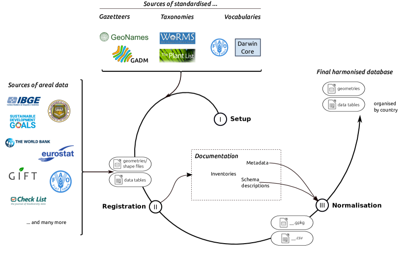
Figure 1: Flow-chart of the general workflow of data integration using arealDB. In stage 1, tables containing standardised terms for all variables of interest are read in to establish an ontological basis. In stage 2, data tables and geometries that have been downloaded from various data sources are registered. In stage 3, those files are harmonised and integrated into the final database. The shown data sources, gazetteers, taxonomies and vocabularies are an exemplary, non exhaustive list of sources that can be handled with arealDB.

2.1 Project setup

An areal database is started with the function setPath(), which creates the standardised directory structure in which the database is stored (Fig. 2a). All further operations within arealDB that rely on a path are then relative to this database directory. Any areal database typically contains a set of variables that identify the observed areal units, such as the unit names. However, it would also include other variables that identify the observed phenomenon, such as timesteps, socioeconomic groups of people, agricultural or other commodities or biological species. The function setVariables() is used to setup the variables that are used in a project to handle lexical translation and semantic harmonisation of the terms of those variables (Fig. 2b). It creates, by default, the skeleton of two files per variable and database, (1) an index table, which relates the variables’ terms to an ID and ancillary information and (2) a translation table, which relates terms in foreign languages and semantics to the target language/ontology. To utilize index tables, an input table that contains term-ID pairs is indispensable and translation tables do not have to, but can be provided with standardised translations of the target variables, which can help improving consistency and data quality (Fig. 1).

Sources of such standardised tabular information may be, for example, gazetteers such as GeoNames (GeoNames (2019)) or the ancillary data in the Global Administrative Areas database (GADM) (Hijmans (2019)), biological taxonomies such as The Plant List (The Plant List (2013)), WoRMS (Horton et al. (2019)) or the IUCN Red List (IUCN (2019)), or standardised ontologies, such as those offered by FAOSTAT (FAO (2019)), the Darwin Core (Wieczorek et al. (2012)), the Humboldt Core (Guralnick et al. (2018)), or the Land Administration Domain Model(Lemmen et al. (2015)).

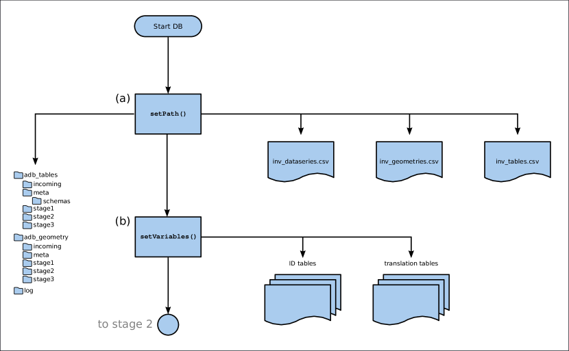
Figure 2: Flow-chart of the project setup. (a) The function setPath()! initiates the project by creating a directory structure in which the files are stored and by creating the inventory tables for data-series, geometries and census tables. (b) The function setVariables()! creates index and translation tables for all variables that should be handled in this project.

2.2 Data registration

An important aspect to ensure the quality of an integrated database is provenance documentation. This allows tracing errors that may show only in the final database to the specific source datasets or to a certain modification process. Documenting provenance requires that the input state of a dataset, as well as procedural metadata that become available as a side-product in the evolution from input to output data, be known.

Thus, the second stage in integrating data with arealDB is to create an inventory of the relevant files and to record metadata on the initial state of data, such as original file names, file locations, licenses and the arrangement of data tables (this process is called registering in arealDB). The arrangement of data tables is managed via the independent R-package tabshiftr (Ehrmann and Rümmler (2020)). Here, so-called schema descriptions are defined, where the table-specific arrangement is described by the position (columns and rows) of data components in the table, which is the basis for automatically reshaping the files in stage 3.

arealDB thoroughly documents metadata on three kinds of information, data-series, geometries and data tables. Data-series are collections of data that are provided by the same source and which share more or less the same tabular arrangement and organisational logic. By documenting the data-series, one mostly documents information about a particular data provider and creates a tag that is common for input data that "belong together" and typically share a common structure. That information will eventually be documented in the three inventory tables of the respective names inv_dataseries.csv, inv_geometries.csv and inv_tables.csv. None of these inventory tables ever need to be modified by hand, as all information documented here is managed automatically.

A new data-series is registered with the function regDataseries(), before geometries and data tables, which are registered with the functions regGeometry() and regTable() (Fig. 3). The functions carry out the following operations:

• check the arguments for valid values and consistency,.

• oversee that the individual items are transformed to the target format with standard names and stored in the correct directory,

• create IDs for all items and insert the provided metadata into the respective inventory tables.

Figure 3: Flow-chart of the registration procedure. (a) The function regDataseries()! is used to document the various data-series (both, of data tables and geometries) that are provided by the data source. (b) The function regGeometry()! is then used to register all geometry files that have been downloaded. (c) Finally, the function regTable()! is used to register all census tables that have been downloaded, and to relate the census tables to data-series and geometries. The registered files are stored in the folders "/adb_geometries/stage2"! and "/adb_tables/stage2"!.

2.3 Data normalisation

The third and final step to integrate areal data consists of reshaping and harmonising the output of stage 2 (Fig. 4) and this process is called normalising in arealDB (Codd (1990)). This final step is crucial, since at stage 2, there is still no guarantee that names of territorial units in geometries are associated with those in data tables or that areal data are georeferenced, that variables are provided in the same language across several sources, or that data tables are provided in a compatible arrangement.

Geometries are typically provided as shape or geopackage files, which have already been optimised for interoperability, and where it is thus sufficient to know which columns in the attribute table contain names of the territorial units (see regGeometry()). The function normGeometry() builds harmonised geometry collections with regard to coordinate reference system, as well as semantically interoperable attribute tables. The overall procedure is detailed in Fig. A.1.

There is no generally accepted way of recording data in tables so that these can be vastly more complex or messy than geometries, and hence require schema descriptions. The schema descriptions that have been recorded at stage 2 document accurate positions of variables held in data tables. The function normTable() utilises those schemas, in concert with the function tabshiftr::reorganise(), to reshape the data into syntactically interoperable tables. It utilises, furthermore, the functions matchUnits() and matchVars() to harmonise labels of territorial units and the levels of identifying variables to end up with semantically interoperable data tables.

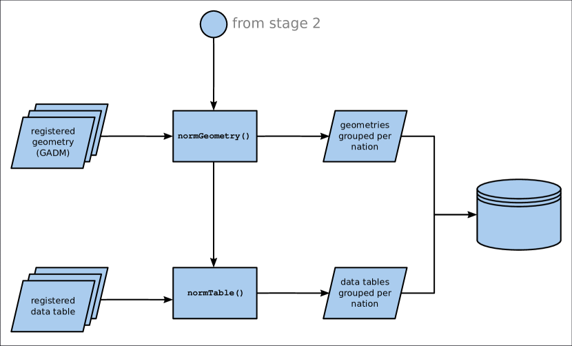
Figure 4: Flow-chart of the normalisation procedure. The function normGeometry()! groups geometries per nation and creates the administrative hierarchy ID (ahID). The function normTable()! reshapes the data tables into tidy format, calls matchUnits()! to assign ahID to the areal data and groups the tables per nation. The normalised files are stored in the folders "/adb_geometries/stage3"! and "adb_tables/stage3"!

2.4 The administrative hierarchy

Geometries in arealDB are assigned a unique ID for each territorial unit at each administrative level. This requires, first of all, an initial geometry dataset from which this administrative hierarchy ID (ahID) can be constructed, and which must thus include information on the hierarchical arrangement of the territorial units. At each administrative level a three-digit ID is assigned to the alphabetically sorted unit names. When descending into a lower level, that ID is restarted at 0 within each parent unit. For instance, Tartu County in Estonia has the ahID 070013, as Estonia is the 70th country (alphabetically) and Tartu County the 13th county within Estonia.

2.5 Translating terms

When handling data from sources that span large spatial extents, these are likely only present in different languages. However, terms may be provided not only in different languages (sensu stricto), but also with distinct semantic meanings. For example, the concept of patch of land that is dominated by grassy vegetation and on which cattle graze, could be called "pasture" (British English), but also "rangeland" (American English), and is called "pastagem" in Portuguese. The language translation "pastagem <-> pasture" from Portuguese to English is functionally similar to the semantic translation "rangeland <-> pasture". Both examples are cases of many-to-one translations because terms in different languages (sensu lato) refer to the same term in the target language. Additionally, in a particular dataset, the term "pasture" might refer to anything from atificially maintained grassland managed for livestock grazing to natural grassland (i.e., with or without livestock). Ideally, these different meanings will become evident from available metadata. In arealDB, an individual term is allowed to refer to different concepts, depending on where it originates, which constitutes a one-to-many semantic translation.

Many-to-one translations are handled quite straightforwardly, in that the target value is repeated in the column target for each translation and terms that refer to it are recorded in the column origin (Tab. 2). One-to-many translations are provided, in the column source, either with geoID or tabID, depending on whether the terms originate from geometries or tables, and in ID with the respective ID.

Table 2: A translation table that includes (a) many-to-one translations (lines 1 and 2) and a case of one-to-many translations (line 3), as well as (b) language (line 1) and semantic (lines 2 and 3) translations of the term ’pasture’.

origin	target	source	ID	notes
pastagem	pasture
rangeland	pasture
pasture	grassland	tabID	3
…

The function translateTerms() manages all translations by comparing new terms individually and explicitly with the translation tables that have been created in stage 1. The user is provided with an interface that suggests a range of terms pre-selected from the translation table via approximate string matching (fuzzy matching). The missing translations then have to be provided by the user, so that the new terms can finally be compared against the look-up section of the translation table to check for consistent translations.

3 Results

We have tested the described functionalities on several dozen agricultural and forestry census datasets from most countries of the American continent. These data represent many of the challenges outlined in Tab. 1, including different table arrangements of the areal data, dissimilar variables provided in different languages and associations to geometries, if they were provided at all, in distinct spatial projections. In Appendix A, we exemplarily showcase the integration of data on the soybean harvested area for Brazil and the US. Downstream applications, such as maps of the spatial patterns (Fig. 5 and Appendix B) or explorative analysis, can profit from the relative ease of accessing all data in a database that has been built with arealDB at once.

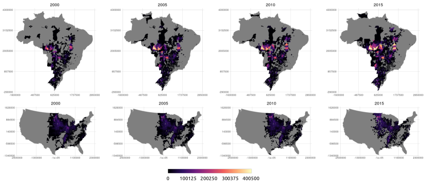
Figure 5: Choropleth maps of the final, integrated database. The maps have been created with the simple code snippet that is shown in Appendix B. The standardised geometries and data tables were read in with a loop through all countries of interest and the maps were created with another loop through the years of interest to plot the data via the R-package geometr (Ehrmann (2019)).

The schema descriptions for each input dataset are central to this workflow. They record the type of each variable, the locationin a spreadsheet (row, col) at which the variable is and other metadata that are relevant to reshape the table.

At stage 2, the Brazilian dataset is organised in a systematic way, however the arrangement is rather complicated (Listing 1). First of all, the spreadsheet contains a metadata header in the first three rows so that the origin of the table is at the fourth row in the first column. The values of the identifying variables "years" and "commodities" and the target variable "harvested" are stored in the same columns. Moreover, states (al2) and municipalities (al3) are combined in the first column, so that this column has to be split. The names of the states are abbreviated, requiring translation to correct names (e.g., "RO <-> Rondônia").

⬇

library(readr)

# input and schema for Brazil

read_csv(file = paste0(dbPath, "/adb_tables/stage2/processed/bra_3_soy_2000_2018_ibge.csv"), col_names = FALSE)

#> # A tibble: 5,569 x 20

#> X1 X2 X3 X4 X5 X6 X7 X8 X9 X10

#> <chr> <chr> <chr> <chr> <chr> <chr> <chr> <chr> <chr> <chr>

#> 1 Tabel NA NA NA NA NA NA NA NA NA

#> 2 Varia NA NA NA NA NA NA NA NA NA

#> 3 Munic Ano x NA NA NA NA NA NA NA NA

#> 4 NA 2000 2001 2002 2003 2004 2005 2006 2007 2008

#> 5 NA Soja Soja Soja Soja Soja Soja Soja Soja Soja

#> 6 Alta - - - - 100 - - - -

#> 7 Ariqu - - 450 - - - 50 - -

#> 8 Cabix 200 486 600 1500 1500 5370 7500 6000 7000

#> 9 Cacoa - - - - - - - - -

#> 10 Cerej 2700 3353 3400 4516 7184 8000 18000 16200 18000

#> # with 5,559 more rows, and 10 more variables: X11 <chr>,

#> # X12 <chr>, X13 <chr>, X14 <chr>, X15 <chr>, X16 <chr>,

#> # X17 <chr>, X18 <chr>, X19 <chr>, X20 <chr>

read_rds(path = paste0(dbPath, "/adb_tables/meta/schemas/schema_1.rds"))

#> 1 cluster

#> origin: 4|1 (top|left)

#>

#> variable type row col rel dist

#> ------------- -------- ----- ------ ----- ------

#> al2 id 1 F F

#> al3 id 1 F F

#> year id 4 2:20 F F

#> commodities id 5 2:20 F F

#> harvested measured 2:20 F F

Listing 1: Schema description of the Brazilian dataset

The US dataset, on the other hand, is already "tidy" at stage 2, i.e., all variables are recorded in individual columns that simply have to be selected, and no lexical or ontological translations are required (Listing 2).

⬇

read_csv(file = paste0(dbPath, "/adb_tables/stage2/processed/usa_3_soy_2000_2018_usda.csv"), col_names = FALSE)

#> # A tibble: 30,143 x 21

#> X1 X2 X3 X4 X5 X6 X7 X8 X9 X10

#> <chr> <chr> <chr> <chr> <chr> <chr> <chr> <chr> <chr> <chr>

#> 1 Progr Year Period Week Geo State Stat Ag D Ag D Coun

#> 2 SURVEY 2018 YEAR NA COUN ALAB 1 BLAC 40 DALL

#> 3 SURVEY 2018 YEAR NA COUN ALAB 1 BLAC 40 ELMO

#> 4 SURVEY 2018 YEAR NA COUN ALAB 1 BLAC 40 OTHE

#> 5 SURVEY 2018 YEAR NA COUN ALAB 1 BLAC 40 PERRY

#> 6 SURVEY 2018 YEAR NA COUN ALAB 1 BLAC 40 SUMT

#> 7 SURVEY 2018 YEAR NA COUN ALAB 1 COAS 50 BALD

#> 8 SURVEY 2018 YEAR NA COUN ALAB 1 COAS 50 OTHE

#> 9 SURVEY 2018 YEAR NA COUN ALAB 1 MOUN 20 BLOU

#> 10 SURVEY 2018 YEAR NA COUN ALAB 1 MOUN 20 CHER

#> # with 30,133 more rows, and 11 more variables: X11 <chr>,

#> # X12 <chr>, X13 <chr>, X14 <chr>, X15 <chr>, X16 <chr>,

#> # X17 <chr>, X18 <chr>, X19 <chr>, X20 <chr>, X21 <chr>

read_rds(path = paste0(dbPath, "/adb_tables/meta/schemas/schema_2.rds"))

#> 1 cluster (whole spreadsheet)

#>

#> variable type row col rel dist

#> ------------- -------- ----- ----- ----- ------

#> al2 id 6 F F

#> al3 id 10 F F

#> year id 2 F F

#> commodities id 16 F F

#> harvested measured 20 F F

Listing 2: Schema description of the US dataset

After normalising (at stage 3), both tables share the same arrangement, where every information is encoded by IDs that point either to metadata (tabID, geoID), territorial units (ahID), or to commodities (faoID).

⬇

read_csv(file = paste0(dbPath, "/adb_tables/stage3/brazil.csv"), col_types = "iiiiidi") %>%

summary()

#> id tabID geoID ahID

#> Min. : 1 Min. :1 Min. :5 Min. :32001001

#> 1st Qu.:24648 1st Qu.:1 1st Qu.:5 1st Qu.:32011029

#> Median :49296 Median :1 Median :5 Median :32015197

#> Mean :49296 Mean :1 Mean :5 Mean :32015793

#> 3rd Qu.:73944 3rd Qu.:1 3rd Qu.:5 3rd Qu.:32021306

#> Max. :98591 Max. :1 Max. :5 Max. :32027137

#>

#> year harvested faoID

#> Min. :2000 Min. : 0 Min. :236

#> 1st Qu.:2004 1st Qu.: 460 1st Qu.:236

#> Median :2009 Median : 2950 Median :236

#> Mean :2009 Mean : 12388 Mean :236

#> 3rd Qu.:2014 3rd Qu.: 11500 3rd Qu.:236

#> Max. :2018 Max. :411224 Max. :236

#> NA’s :65529

read_csv(file = paste0(dbPath, "/adb_tables/stage3/united states of america.csv"), col_types = "iiiiidi") %>%

summary()

#> id tabID geoID ahID

#> Min. : 1 Min. :2 Min. :3 Min. :238001001

#> 1st Qu.: 6871 1st Qu.:2 1st Qu.:3 1st Qu.:238016074

#> Median :13740 Median :2 Median :3 Median :238025054

#> Mean :13740 Mean :2 Mean :3 Mean :238026647

#> 3rd Qu.:20610 3rd Qu.:2 3rd Qu.:3 3rd Qu.:238036065

#> Max. :27480 Max. :2 Max. :3 Max. :238050074

#> year harvested faoID

#> Min. :2000 Min. : 40.47 Min. :236

#> 1st Qu.:2004 1st Qu.: 2954.21 1st Qu.:236

#> Median :2008 Median : 12788.07 Median :236

#> Mean :2009 Mean : 20302.90 Mean :236

#> 3rd Qu.:2013 3rd Qu.: 33108.34 3rd Qu.:236

#> Max. :2018 Max. :218125.56 Max. :236

Listing 3: Summary of the core table of the harmonised and integrated database

4 Discussion

The present R package arealDB provides so far missing software for harmonising and integrating areal data across multiple heterogeneous sources into a single, consistent database (Fig. 6). By guiding users through the three stages ’project setup’, ’data registration’ and ’data normalisation’ , embedded into a collaborative and transparent software environment (Lowndes et al. (2017)), arealDB substantially improves the speed, scientific accuracy, and reproducibility of integrating areal data.

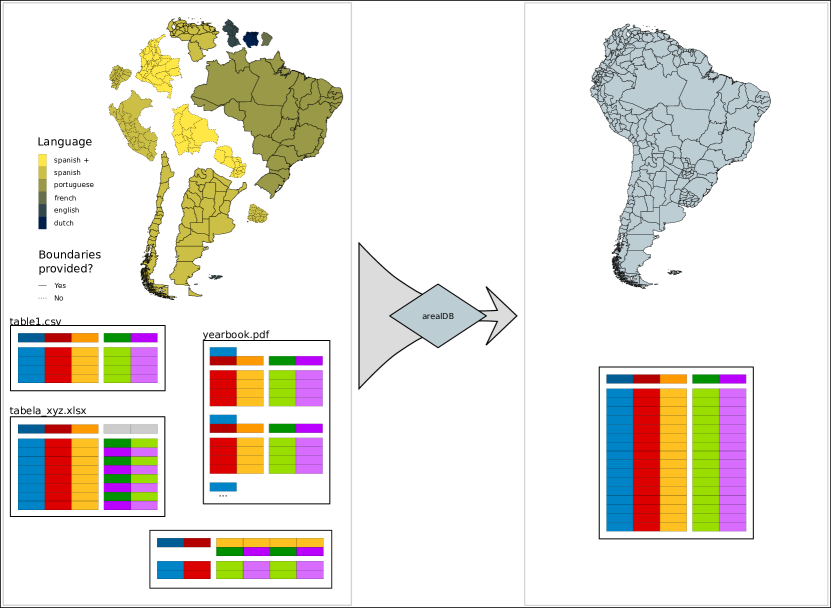
Figure 6: Schematic overview of the purpose of arealDB. Both, data tables that are disorganised and messy and that are based on different languages and concepts, as well as distinctly organised geometric datasets are harmonised and integrated into one consistent database.

Lacking such a tool, many data integrators have thus far gone through a highly time-consuming and error-prone process of opening individual input datasets in Excel, translating variables "by hand", and reshaping tables by copying relevant data from one spreadsheet into another, typically without any provenance documentation. More sophisticated workflows based on advanced tools, such as lookup and pivot tables or programmable statistical/data management tools often require custom-scripted solutions for the different, heterogeneous input data-sets. arealDB, by contrast, merely requires that users document metadata, provide translation tables and specify a schema description for each dataset.

4.1 Handling geometries

Using arealDB, each individual areal data table may be linked to a different geometry dataset. This helps to avoid political and other assumptions where more than one source of areal data exists for territorial units, for example in cases of disputed areas or administrative changes. Data that refer to such disparate geometry sources can coexist in a database without biasing downstream analyses that are sensitive to the areas of measurement units (e.g., when estimating ecological scaling relationships from species checklists; (Kreft and Jetz (2007); Keil and Chase (2019)). Where such considerations are not an issue, datasets may be linked to standardised geometries, such as GADM (Hijmans (2019)).

Currently, arealDB matches areal data via an internal assessment of the geographical overlap of geometries (using the R package sf (Pebesma (2018)); see flowchart in Appendix C). This procedure could be further refined by additionally incorporating functions that can automatically detect and handle temporal changes of territorial units (Bernard et al. (2018)). However, as all raw input geometries are retained in the final database, more sophisticated procedures for matching recorded geometries may be applied alongside arealDB’s own functions.

Another common challenge in matching territorial units lies in names that are shared by multiple territorial units located in different nations and at different administrative levels. For example, the term ’Santa Cruz’ may refer to city districts, municipalities, departments, or other units in over twenty different nations. arealDB addresses this issue by matching territorial unit names to geometries hierarchically.

4.2 Documenting metadata

Even arealDB is still prone to some human error, mostly related to correctly reading in the required files and information. arealDB’s system of unique IDs ensures that all data values can be linked to metadata on their input tables, associated geometries, and original data sources. Hence, inconsistencies that may still exist in an output database are fully traceable, due to the metadata collected while collating the database (Henzen et al. (2013)). Moreover, the relational setup of the resulting database allows that database management software can retrieve metadata on all harmonised datasets (e.g., the recorded number of entities or observations, or value ranges) and make those and other metadata available also to other tools and environments.

4.3 Interoperability

arealDB was primarily designed for the purpose of integrating heterogeneous areal data within a given knowledge domain. However, by storing all variables in the same data structure, the tools provided here enable areal databases that are syntactically interoperable across domains. The areal data in each and every output table of arealDB have a value of ahID (Code-Listing 3) that is by default always derived from the same spatial basis, the GADM dataset. Merely areal data for which ahID was derived from specific non-GADM geometries may deviate from a common list of ahID values. This means that areal databases from several distinct domains (for instance, human health and biodiversity) that have all been built with the same geometries dataset can simply be joined via ahID to combine information on the distinct topics within a consistent database and facilitate interdisciplinary applications (Otto et al. (2015)).

While arealDB enables such data integration technically, the endeavour of actually integrating databases across knowledge domains in a meaningful way hinges crucially on advances in ontological standardisation to come up with concepts that are valid simultaneously across knowledge domains (van den Brink et al. (2017)).

5 Conclusions

arealDB provides a range of tools that standardise the process of integrating heterogeneous areal data sources into a single, harmonised database, removing hurdles that come with high resource and time requirements. It enables users that may lack the necessary background knowledge to address the majority of the anticipated issues in setting up a coherent workflow of data integration. This helps in homogenising data collection methodologies, which is urgently needed to tackle data management strategies that are able to deal with vast amounts of heterogeneous data (Otto et al. (2015)).

The tools presented here allow to process any areal data, such as socioeconomic census and survey data, ecological checklist data, data on infectious diseases, (sub-)national indicator data, cadastral parcel data, and many more. arealDB lowers the effort to surpass barriers of the spatial, temporal or thematic scope of single data sources. This can enable many exciting and easy to set-up applications at the pan-regional and global scale, supporting data-integration needs across application domains and progressing towards multiple Sustainable Development Goals.

6 Acknowledgements

CM acknowledges funding by the Volkswagen Foundation via a Freigeist Fellowship. SE acknowledges funding by iDiv via the Flexpool mechanism (FZT-118, DFG).

7 Appendix

• Appendix A: Replication Script

• Appendix B: Downstream Application

• Appendix C: Normalise Geometries

References

- Baumer (2017) Benjamin S Baumer. A grammar for reproducible and painless extract-transform-load operations on medium data. Journal of Computational and Graphical Statistics, 28(2):256–264, 2017. doi: 10.1080/10618600.2018.1512867.
- Bernard et al. (2018) Camille Bernard, Christine Plumejeaud-Perreau, Marlène Villanova-Oliver, Jérôme Gensel, and Hy Dao. An ontology-based algorithm for managing the evolution of multi-level territorial partitions. In Proceedings of the 26th ACM SIGSPATIAL International Conference on Advances in Geographic Information Systems, pages 456–459. ACM, 2018. doi: 10.1145/3274895.3274944.
- Codd (1990) EF Codd. The Relational Model for Database Management: Version 2. Addison-Wesley Longman Publishing Co., Inc., Boston, MA, USA, 1990. ISBN 0-201-14192-2.
- De Giacomo et al. (2018) Giuseppe De Giacomo, Domenico Lembo, Maurizio Lenzerini, Antonella Poggi, and Riccardo Rosati. Using ontologies for semantic data integration. In A Comprehensive Guide Through the Italian Database Research Over the Last 25 Years, pages 187–202. Springer, 05 2018. ISBN 978-3-319-61892-0. doi: 10.1007/978-3-319-61893-7_11.
- Debroy et al. (2018) Vidroha Debroy, Lance Brimble, and Matt Yost. Newtl: engineering an extract, transform, load (etl) software system for business on a very large scale. In Proceedings of the 33rd Annual ACM Symposium on Applied Computing, pages 1568–1575. ACM, 2018.
- Du et al. (2013) Heshan Du, Natasha Alechina, Mike Jackson, and Glen Hart. Matching formal and informal geospatial ontologies. In Geographic information science at the heart of Europe, pages 155–171. Springer, 2013. doi: 10.1007/978-3-319-00615-4_9. URL https://link.springer.com/chapter/10.1007/978-3-319-00615-4_9.
- Ehrmann (2019) Steffen Ehrmann. geometr: Generate and Modify Interoperable Geometric Shapes, 2019. URL https://github.com/EhrmannS/geometr. R package version 0.2.2.
- Ehrmann and Rümmler (2020) Steffen Ehrmann and Arne Rümmler. rectifyr: Reshape disorganised messy tables, 2020. URL https://gitlab.com/luckinet/software/rectifyr. R package version 0.1.2.
- FAO (2019) FAO. Faostat, 2019. URL http://www.fao.org/faostat.
- GeoNames (2019) GeoNames. Geonames, 2019. URL http://www.geonames.org.
- Guralnick et al. (2018) Robert Guralnick, Ramona Walls, and Walter Jetz. Humboldt core–toward a standardized capture of biological inventories for biodiversity monitoring, modeling and assessment. Ecography, 41(5):713–725, 2018. URL https://onlinelibrary.wiley.com/doi/full/10.1111/ecog.02942.
- Henzen et al. (2013) Christin Henzen, Stephan Mäs, and Lars Bernard. Provenance information in geodata infrastructures. In Geographic Information Science at the Heart of Europe, volume 2013, pages 133–151. Springer International Publishing, 05 2013. ISBN 978-3-319-00615-4. doi: 10.1007/978-3-319-00615-4_8. URL https://doi.org/10.1007/978-3-319-00615-4_8.
- Hijmans (2019) Robert J Hijmans. Global administrative areas, 2019. URL www.gadm.org.
- Horridge (2011) M Horridge. A practical guide to building owl ontologies using protégé 4 and co-ode tools edition 1.3. retrieved march 10, 2013, 2011.
- Horton et al. (2019) T. Horton, A. Kroh, S. Ahyong, N. Bailly, C.B. Boyko, S.N. Brandão, S. Gofas, J.N.A. Hooper, F. Hernandez, O. Holovachov, J. Mees, T.N. Molodtsova, G. Paulay, W. Decock, S. Dekeyzer, T. Lanssens, L. Vandepitte, B. Vanhoorne, K. Verfaille, R. Adlard, P. Adriaens, S. Agatha, K.J. Ahn, N. Akkari, B. Alvarez, G. Anderson, M.V. Angel, C. Arango, T. Artois, S. Atkinson, R. Bank, A. Barber, J.P. Barbosa, I. Bartsch, D. Bellan-Santini, J. Bernot, A. Berta, T.N. Bezerra, R. Bieler, S. Blanco, I. Blasco-Costa, M. Blazewicz, P. Bock, R. Böttger-Schnack, P. Bouchet, N. Boury-Esnault, G. Boxshall, R. Bray, B. Breure, N.L. Bruce, S. Cairns, P. Cárdenas, E. Carstens, B.K. Chan, T.Y. Chan, L. Cheng, M. Churchill, C.O. Coleman, A.G. Collins, L. Corbari, R. Cordeiro, A. Cornils, M. Coste, M.J. Costello, K.A. Crandall, F. Cremonte, T. Cribb, S. Cutmore, F. Dahdouh-Guebas, M. Daly, M. Daneliya, J.C. Dauvin, P. Davie, C. De Broyer, S. De Grave, V. de Mazancourt, N.J. de Voogd, P. Decker, W. Decraemer, D. Defaye, J.L. d’Hondt, S. Dippenaar, M. Dohrmann, J. Dolan, D. Domning, R. Downey, L. Ector, U. Eisendle-Flöckner, M. Eitel, S.C.d. Encarnação, H. Enghoff, J. Epler, C. Ewers-Saucedo, M. Faber, S. Feist, D. Figueroa, J. Finn, C. Fišer, E. Fordyce, W. Foster, J.H. Frank, C. Fransen, H. Furuya, H. Galea, O. Garcia-Alvarez, R. Garic, R. Gasca, S. Gaviria-Melo, S. Gerken, D. Gibson, R. Gibson, J. Gil, A. Gittenberger, C. Glasby, A. Glover, S.E. Gómez-Noguera, D. González-Solís, D. Gordon, M. Grabowski, C. Gravili, J.M.. Guerra-García, R. Guidetti, M.D. Guiry, K.A. Hadfield, E. Hajdu, J. Hallermann, B.W. Hayward, E. Hendrycks, D. Herbert, A. Herrera Bachiller, J.s. Ho, M. Hodda, J. Høeg, B. Hoeksema, R. Houart, L. Hughes, M. Hyžný, L.F.M. Iniesta, T. Iseto, S. Ivanenko, M. Iwataki, R. Janssen, G. Jarms, D. Jaume, K. Jazdzewski, C.D. Jersabek, P. Jóźwiak, A. Kabat, Y. Kantor, I. Karanovic, B. Karthick, Y.H. Kim, R. King, P.M. Kirk, M. Klautau, J.P. Kociolek, F. Köhler, J. Kolb, A. Kotov, A. Kremenetskaia, R.M. Kristensen, M. Kulikovskiy, S. Kullander, G. Lambert, D. Lazarus, F. Le Coze, S. LeCroy, D. Leduc, E.J. Lefkowitz, R. Lemaitre, Y. Liu, A.N. Lörz, J. Lowry, T. Ludwig, N. Lundholm, E. Macpherson, L. Madin, C. Mah, B. Mamo, T. Mamos, R. Manconi, G. Mapstone, P.E. Marek, B. Marshall, D.J. Marshall, P. Martin, R. Mast, C. McFadden, S.J. McInnes, T. Meidla, K. Meland, K.L. Merrin, C. Messing, D. Miljutin, C. Mills, Ø. Moestrup, V. Mokievsky, F. Monniot, R. Mooi, A.C. Morandini, R. Moreira da Rocha, F. Moretzsohn, C. Morrow, J. Mortelmans, J. Mortimer, L. Musco, T.A. Neubauer, E. Neubert, B. Neuhaus, P. Ng, A.D. Nguyen, C. Nielsen, T. Nishikawa, J. Norenburg, T. O’Hara, D. Opresko, M. Osawa, H.J. Osigus, Y. Ota, B. Páll-Gergely, D. Patterson, H. Paxton, R. Peña-Santiago, V. Perrier, W. Perrin, I. Petrescu, B. Picton, J.F. Pilger, A.B. Pisera, D. Polhemus, G.C. Poore, M. Potapova, P. Pugh, G. Read, M. Reich, J.D. Reimer, H. Reip, M. Reuscher, J.W. Reynolds, I. Richling, F. Rimet, P. Ríos, M. Rius, D.C. Rogers, G. Rosenberg, K. Rützler, K. Sabbe, J. Saiz-Salinas, S. Sala, S. Santagata, S. Santos, E. Sar, A. Satoh, T. Saucède, H. Schatz, B. Schierwater, A. Schmidt-Rhaesa, S. Schneider, C. Schönberg, P. Schuchert, A.R. Senna, C. Serejo, S. Shaik, S. Shamsi, J. Sharma, W.A. Shear, N. Shenkar, A. Shinn, M. Short, J. Sicinski, P. Sierwald, E. Simmons, F. Sinniger, D. Sivell, B. Sket, H. Smit, N. Smit, N. Smol, J.F.. Souza-Filho, J. Spelda, W. Sterrer, E. Stienen, P. Stoev, S. Stöhr, M. Strand, E. Suárez-Morales, M. Summers, L. Suppan, C. Suttle, B.J. Swalla, S. Taiti, M. Tanaka, A.H. Tandberg, D. Tang, M. Tasker, J. Taylor, J. Taylor, A. Tchesunov, H. ten Hove, J.J. ter Poorten, J.D. Thomas, E.V. Thuesen, M. Thurston, B. Thuy, J.T. Timi, T. Timm, A. Todaro, X. Turon, S. Tyler, P. Uetz, J. Uribe-Palomino, S. Utevsky, J. Vacelet, D. Vachard, W. Vader, R. Väinölä, B. Van de Vijver, S.E. van der Meij, T. van Haaren, R.W. van Soest, A. Vanreusel, V. Venekey, M. Vinarski, R. Vonk, C. Vos, G. Walker-Smith, T.C. Walter, L. Watling, M. Wayland, T. Wesener, C.E. Wetzel, C. Whipps, K. White, U. Wieneke, D.M. Williams, G. Williams, R. Wilson, A. Witkowski, J. Witkowski, N. Wyatt, C. Wylezich, K. Xu, J. Zanol, W. Zeidler, and Z. Zhao. World register of marine species (worms). =http://www.marinespecies.org, 2019. URL http://www.marinespecies.org. Accessed: 2019-09-11.
- IUCN (2019) IUCN. The iucn red list of threatened species, 2019. URL http://www.iucnredlist.org. Version 2019-2.
- Keil and Chase (2019) Petr Keil and Jonathan M Chase. Global patterns and drivers of tree diversity integrated across a continuum of spatial grains. Nature ecology & evolution, 3(3):390, 2019. doi: 10.1038/s41559-019-0799-0.
- Kreft and Jetz (2007) Holger Kreft and Walter Jetz. Global patterns and determinants of vascular plant diversity. Proceedings of the National Academy of Sciences, 2007. doi: 10.1073/pnas.0608361104. URL https://www.pnas.org/content/104/14/5925.
- Lemmen et al. (2015) Christiaan Lemmen, Peter Van Oosterom, and Rohan Bennett. The land administration domain model. Land use policy, 49:535–545, 2015. doi: 10.1016/j.landusepol.2015.01.014. URL https://www.sciencedirect.com/science/article/pii/S0264837715000174?via%3Dihub.
- Lowndes et al. (2017) Julia S Stewart Lowndes, Benjamin D Best, Courtney Scarborough, Jamie C Afflerbach, Melanie R Frazier, Casey C O’Hara, Ning Jiang, and Benjamin S Halpern. Our path to better science in less time using open data science tools. Nature ecology & evolution, 1(6):1–7, 2017. doi: 10.1038/s41559-017-0160.
- Otto et al. (2015) Ilona M Otto, Anne Biewald, Dim Coumou, Georg Feulner, Claudia Köhler, Thomas Nocke, Anders Blok, Albert Gröber, Sabine Selchow, David Tyfield, et al. Socio-economic data for global environmental change research. Nature Climate Change, 5(6):503, 2015. doi: 10.1038/nclimate2593. URL https://www.nature.com/articles/nclimate2593.pdf.
- Pebesma (2018) Edzer Pebesma. Simple Features for R: Standardized Support for Spatial Vector Data. The R Journal, 10(1):439–446, 2018. doi: 10.32614/RJ-2018-009. URL https://doi.org/10.32614/RJ-2018-009.
- Petersen and Ekstrøm (2019) Anne Helby Petersen and Claus Thorn Ekstrøm. datamaid: Your assistant for documenting supervised data quality screening in r. Journal of Statistical Software, 90(1):1–38, 2019.
- The Plant List (2013) The Plant List. The plant list, 2013. URL http://www.theplantlist.org/. Version 1.1.
- van den Brink et al. (2017) Linda van den Brink, Paul Janssen, Wilko Quak, and Jantien Stoter. Towards a high level of semantic harmonisation in the geospatial domain. Computers, Environment and Urban Systems, 62:233–242, 2017. doi: 10.1016/j.compenvurbsys.2016.12.002.
- Wickham (2014) Hadley Wickham. Tidy data. Journal of Statistical Software, 59(10):1–23, 2014. doi: 10.18637/jss.v059.i10. URL https://www.jstatsoft.org/article/view/v059i10.
- Wieczorek et al. (2012) John Wieczorek, David Bloom, Robert Guralnick, Stan Blum, Markus Döring, Renato Giovanni, Tim Robertson, and David Vieglais. Darwin core: an evolving community-developed biodiversity data standard. PloS One, 7(1):e29715, 2012. doi: 10.1371/journal.pone.0029715. URL https://journals.plos.org/plosone/article/file?id=10.1371/journal.pone.0029715&type=printable.