Learning Interpretable Disease
Self-Representations for Drug Repositioning

Abstract

Drug repositioning is an attractive cost-efficient strategy for the development of treatments for human diseases. Here, we propose an interpretable model that learns disease self-representations for drug repositioning. Our self-representation model represents each disease as a linear combination of a few other diseases. We enforce proximity in the learnt representations in a way to preserve the geometric structure of the human phenome network — a domain-specific knowledge that naturally adds relational inductive bias to the disease self-representations. We prove that our method is globally optimal and show results outperforming state-of-the-art drug repositioning approaches. We further show that the disease self-representations are biologically interpretable.

1 Introduction

New drug discovery and development presents several challenges including high attrition rates, long development times, and substantial costs (Ashburn and Thor, 2004). Drug repositioning, the process of finding new therapeutic indications for already marketed drugs, has emerged as a promising alternative to new drug development. It involves the use of de-risked compounds in human, which translates to lower development costs and shorter development times (Pushpakom et al., 2018).

A wide range of computational approaches has been proposed to predict novel indications for existing drugs. The common assumption underlying these methods is that there is biological or pharmacological relational information between drugs, e.g., chemical structure, and between diseases, e.g., disease phenotypes, that can be exploited for the prediction task. Current methods typically rely on well-defined heuristics and/or hand-crafted features. For instance, the PREDICT (Gottlieb et al., 2011) model extracts drug-disease features from multiple similarity measures, and then trains a logistic regression classifier to predict novel drug indications. Similarly, (Napolitano et al., 2013) obtains features from heterogeneous drug similarity measures and then trains an SVM classifier to predict therapeutic indications of drugs. Other approaches include random walks on bipartite networks (Luo et al., 2016), and low-rank matrix completion-based approaches (Luo et al., 2018).

In this paper, we propose a self-representation learning model for drug repositioning that is able to overcome the limitations of heuristic-based approaches and extend the expressiveness of low-rank factorisation models for matrix completion. Our model builds upon the recent development of high-rank matrix completion based on self-expressive models (SEM) (Elhamifar, 2016), as well as the recent trend of deep learning on graphs (Bronstein et al., 2017; Monti et al., 2017; Hamilton et al., 2017). We propose a geometric SEM model that integrates relational inductive bias about genetic diseases in the form of a disease phenotype similarity graph. Extensive experiments on a standard benchmark dataset show that our method outperforms existing state-of-the-art approaches in drug repositioning, and that the inclusion of relational inductive bias significantly improves the performance while enhancing model interpretability.

2 Geometric Self-Expressive Models (GSEM)

2.1 Regularisation Framework

The goal of self-expressive models (SEM) is to represent datapoints, i.e., diseases, approximately as a linear combination of a small number of other datapoints. Proposed as a framework for simultaneously clustering and completing high-dimensional data lying over the union of low-dimensional subspaces (Fan and Chow, 2017; Wang and Elhamifar, 2018), these models can effectively generalise standard low-rank matrix completion models. Here we cast drug repositioning as a high-rank matrix completion task and propose a model that naturally extends SEM by imposing a relational inductive prior between datapoints. Because of the geometrical structure enforced between datapoints, we refer to our model as Geometric SEM (GSEM).

Let us denote our drug disease matrix for $n$ drugs and $m$ diseases with the matrix $X\in\mathbb{R}^{n\times m}$ (each column is a datapoint) where $x_{ij}=1$ if drug $i$ is associated with disease $j$, and zero otherwise. GSEM aims at learning a sparse zero-diagonal self-representation matrix $C\in\mathbb{R}^{m\times m}$ of coefficients for diseases such that $\hat{X}\approx XC$, where the null diagonal aims at ruling out the trivial solution $C=I$.

To this end, we minimise the following cost function:

$$\begin{split}&\min_{C\geq 0}\,\,\,\underbrace{\frac{1}{2}\|X-XC\|_{F}^{2}}_{\text{self-representation}}+\underbrace{\frac{\beta}{2}\|C\|_{F}^{2}+\lambda\|C\|_{1}}_{\text{sparsity}}+\underbrace{\frac{\alpha}{2}\|C\|_{\mathcal{D},\mathcal{G}}^{2}}_{\text{smoothness}}+\underbrace{\gamma\operatorname{Tr}(C)}_{\text{null diagonal}}\end{split}$$ (1)

where $\|.\|_{F}$ denotes the Frobenius norm, and $\|C\|_{\mathcal{D},G}$ the Dirichlet norm on the graph $\mathcal{G}=(\{1,\ldots,m\},\mathcal{E},W)$, i.e., the weighted undirected graph with edge weights $w_{ij}>0$ if $(i,j)\in\mathcal{E}$ and zero otherwise, representing the similarities between diseases. We further denote the cost function in Eq. (1) by $\mathcal{Q}(C)$. The first term in Eq. (1) is the self-representation constraint, which aims at learning a matrix of coefficients $C$ such that $XC$ is a good reconstruction of the original matrix $X$. The second term is the sparsity constraint, which uses the elastic-net regularisation known to impose sparsity and grouping-effect (Ng, 2004; Zou and Hastie, 2005). The fourth term is a penalty for diagonal elements to prevent the trivial solution $C=I$ by imposing $\mathrm{diag}(C)=0$ (together with $C\geq 0$). Typically, $\gamma\gg 0$ is used. Relational inductive bias between diseases is imposed by the third smoothness term in Eq.1 (Ma et al., 2011; Kalofolias et al., 2014; Monti et al., 2017), incorporating geometric structure into the self-representation matrix $C$ from the disease-disease similarity graph $\mathcal{G}$. Ideally, nearby points in $\mathcal{G}$ should have similar coefficients in $C$, which can be obtained by minimising:

$$\sum_{i,j}G_{ij}\|c_{i}-c_{j}\|^{2}=\operatorname{Tr}(CLC^{T})=\|C\|_{\mathcal{D,G}}^{2}$$ (2)

where $c_{i}$ and $c_{j}$ represent column vectors of $C$ and $L=D-W$ is the graph Laplacian. The parameter $\alpha>0$ in Eq.1 weighs the importance of the smoothness constraint for the prediction. Finally, to favour interpretability of the learned self-representations, we followed (Lee and Seung, 1999) and also imposed a non-negativity constraint on $C$.

2.2 The multiplicative learning algorithm

To minimise Eq. 1, we developed an efficient multiplicative learning algorithm with theoretical guarantees of convergence. Our algorithm consists in iteratively applying the following rule:

$$c_{ij}\leftarrow c_{ij}\frac{(X^{\top}X+\alpha CW)_{ij}}{(X^{\top}XC+\alpha CD+\beta C+\lambda+\gamma I)_{ij}}$$ (3)

We shall prove that the cost function $\mathcal{Q}(C)$ is convex and therefore, our multiplicative rule in Eq. (3) converges to a global minimum.

Lemma 1.

The cost function $\mathcal{Q}(C)$ in Eq. 1 is convex in the feasible region $C\geq 0$.

Proof Sketch.

We need to prove that the Hessian is a positive semi-definite (PSD) matrix. That is, for a non-zero vector $h\in\mathbb{R}^{m}$ the following condition is met $h^{T}\nabla^{2}\mathcal{Q}(C)h\geq 0$. The graph Laplacian is PSD by definition. The remaining terms in the Hessian ($X^{\top}X+\beta I$) are also PSD. Therefore, $\mathcal{Q}(C)$ is convex in $C\geq 0$. ∎

Theorem 1 (Convergence).

The cost function $\mathcal{Q}(C)$ in Eq. (1) converges to a global minimum under the multiplicative update rule in (3).

Proof.

We need to show that our algorithm satisfies the Karush-Khun-Tucker (KKT) complementary conditions, which are both necessary and sufficient conditions for a global solution point given the convexity of the cost function (lemma 1) (Li and Ding, 2006; Boyd and Vandenberghe, 2004). KKT requires $c_{ij}\geq 0$ and $(\nabla\mathcal{Q}(C))_{ij}c_{ij}=0$. The first condition holds with non-negative initialisation of $C$. For the second condition, the gradient is: $\nabla\mathcal{Q}(C)=-X^{\top}X-\alpha CW+X^{\top}XC+\alpha CD+\beta C+\lambda+\gamma I$, and according to the second KKT condition, at convergence $C=C^{*}$ we have $(X^{\top}XC^{*}+\alpha C^{*}D+\beta C^{*}+\lambda+\gamma I)_{ij}c^{*}_{ij}-(X^{\top}X+\alpha C^{*}W)_{ij}c^{*}_{ij}=0$, which is identical to (3). That is, the multiplicative rule converges to a global minimum solution point. ∎

3 Experimental Results

Datasets

Drug-disease associations were obtained from the PREDICT dataset (Gottlieb et al., 2011), a standard benchmark for computational drug repositioning. Our drug-disease matrix $X$ contains $1933$ known drug-disease associations between $593$ drugs (rows) and $313$ genetic diseases (columns). Drugs were extracted from the DrugBank database (Wishart et al., 2018) while diseases were defined using the Online Mendelian Inheritance in Man (OMIM) database (Hamosh et al., 2004). To build the disease-disease graph $\mathcal{G}$, we used the phenotypic disease similarity constructed by (Van Driel et al., 2006). Our adjacency matrix $W$ consists of a dense matrix of $313\times 313$ with values ranging in the interval $[0,1]$.

Settings

Following previous approaches (Gottlieb et al., 2011; Luo et al., 2018), we frame the computational drug repositioning task as a binary classification problem. We used a ten-fold cross-validation procedure while ensuring that all the drugs had at least one association in the training set. For each fold, we used a validation set for hyperparameter tuning ($\lambda,\beta,\alpha$ and $\gamma$). To filter irrelevant relationships between diseases, we also optimised a threshold parameter $\tau$ such that $w_{ij}=0$ if $w_{ij}<\tau$. Given that our data matrix $X$ is highly imbalanced ($1.04\%$ density), we measured the performance of the classifier using the area under the precision recall curve (AUPR) — which has been shown to be more informative than the AUROC in imbalanced scenarios (Saito and Rehmsmeier, 2015) — for varying values of ratio between negative ($0$s) and positive ($1$s) labels. We compared the performance of our method against PREDICT (Gottlieb et al., 2011), a recent low-rank matrix completion model called Drug Repositioning Recommendation System (DRRS) (Luo et al., 2018) and a non-geometric version of our model (with $\alpha=0$, SEM). For both PREDICT and DRRS, we ran the algorithms with the respective similarity measures used in their original papers. An object-oriented implementation of our model, along with datasets to reproduce our study, is available at https://github.com/Noired/GSEM.git.

Performance Evaluation

Figure 1 summarises the performance of the methods. We observed that while GSEM is only marginally better than DRRS and PREDICT in the balanced scenario (negative-to-positive ratio 1:1, AUPR of $0.950\pm 0.010$ for GSEM, $0.947\pm 0.012$ for DRRS and $0.932\pm 0.020$ for PREDICT), it greatly outperforms these competitors in imbalanced scenarios (by 1.0-13.16% at 10:1, 4.67-29.15% at 30:1, 6.48-27.60% at 50:1 and 10.31-33.12% at 100:1). Although PREDICT integrates information from seven heterogeneous similarity measures, it performs poorly with high data imbalance, where, a simple SEM model, which does not use any relational prior between diseases, intriguingly outperforms PREDICT and DRRS by 1.93-23.05% at 50:1 and 6.03-28.84% at 100:1. This means that our high-rank model of $X$ based on self-representations is able to better exploit the intrinsic relationships between diseases inferred from the data matrix $X$ — we checked that indeed the matrix $X$ has a high-rank (rank = $238/313$). The contribution of the relational information between diseases becomes clear when comparing the performances of the GSEM versus SEM model: on average, GSEM outperforms SEM by 4.85% AUPR across all the ratios.

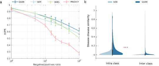
Figure 1: (a) Drug repositioning performance. Mean and standard deviation for AUPR metric computed using ten-fold cross-validation for varying values of negative to positive label ratios (ratio $\in\{1,5,10,15,20,30,40,50,100\}$). Performance of our method (GSEM) is reported, along with that of the state-of-the-art DRRS (Luo et al., 2018), PREDICT (Gottlieb et al., 2011) and standard SEM. Our model performs best in the more realistic unbalanced scenario. (b) Model interpretation. Comparative violin plot of disease self-representation similarities. Diseases were grouped by well-known phenotypic classes. Significance levels between the average intra-class similarities for GSEM and SEM is indicated with asterisks ($p\leq 0.001$, $***$).

4 Model Interpretation

The effectiveness of our model at predicting new disease indications for drugs prompted us to analyse whether the disease self-representations are informative of the biology underlying drug activity. We assessed model interpretability by exploring the extent to which disease self-representations were related to well-known disease classes. We retrieved disease classes from the International Classification of Diseases of the World Health Organization (WHO) (ICD10CM (WHO, 2016)). We only kept diseases belonging to a unique class, and filtered diseases belonging to a class with less than 5 diseases. For 182 diseases, we obtained 11 distinct classes (see Supplementary Materials). We then defined a disease-disease similarity as the cosine similarity of the rows of $\mathcal{S}=(C+C^{T})/2$. For these experiments, we trained our model using all the available data in $X$ and fixed optimal hyper-parameters (see Supplementary Material). Figure 1(b) shows the violin plots of the distribution of similarities for diseases belonging to the same class (intra-class) versus diseases belonging to distinct classes (inter-class), for both GSEM and SEM. We observed that for both GSEM and SEM, the intra-class similarity is significantly higher than the inter-class similarity (Wilcoxon Sum Rank Significance, $p<3.62\times 10^{-107}$ and $p<3.55\times 10^{-249}$ for SEM and GSEM, respectively), meaning that both models learn biologically meaningful self-representations for diseases. However, the intra-class disease self-representation similarity is significantly higher for GSEM than for SEM (Wilcoxon Sum Rank Significance, $p<1.23\times 10^{-174}$), suggesting that our geometric model efficiently integrates the relational phenotypic information between diseases encoded in the human phenome network.

5 Conclusions and Future Work

Inherently interpretable models are critical for applications involving high-stakes decisions such as health care (Rudin, 2019). These are unfeasible to achieve with neural nets, because the learned representations depend on uninterpreted features in other layers (Hinton, 2018). Here we proposed an inherently interpretable model, GSEM, that learns self-representations for diseases. Our model effectively integrates the relational inductive bias from the human phenome network (Van Driel et al., 2006) — better results could possibly be achieved using the (Caniza et al., 2015) disease similarity, which has shown to be effective for the prediction of genes associated to genetic diseases (Cáceres and Paccanaro, 2019). Ongoing research includes the integration of relational inductive bias for drugs as well.

6 Supplementary Material

6.1 Model Implementation

PREDICT

We re-implemented the PREDICT algorithm in Python 3.6. We computed seven drug-disease features using the original data and following the procedure in (Gottlieb et al., 2011). To train the model, we used the LogisticRegression classifier from sklearn.linear_model to obtain the scores for the drug-disease pairs.

DRRS

To run Drug Repositioning Recommender System (Luo et al., 2018), we used the data and code provided in the original publication. DRRS uses two complementary information for the prediction: the 2D Tanimoto chemical similarity for drugs and phenotype similarities for diseases obtained from MimMiner (Van Driel et al., 2006).

GSEM

We implemented our proposed algorithm in Python 3.6. As model learning is based on a multiplicative learning rule similar to that of non-negative matrix factorisation (NMF) (Lee and Seung, 1999, 2001), we followed the recommended guidelines in (Berry et al., 2007) to implement it: (i) $C$ was initialised with weights sampled from a uniform distribution between $[0,b)$, with $b=1\times 10^{-2}$; (ii) a small value $\varepsilon\simeq 1\times 10^{-16}$ was added to the denominator of the learning algorithm to prevent division by zero. The learning rule is iteratively applied until either of the following stopping condition is met: (i) maxiter iterations are completed; (ii) the relative change $\delta^{(t)}$ in the value of $C$ across two subsequent iterations is smaller than a predefined termination tolerance tol (Kearfott and Walster, 2000):

$$\delta^{(t)}=\max_{ij}\left(\frac{|c_{ij}^{(t+1)}-c_{ij}^{(t)}|}{\max_{(i,j)}|c_{ij}^{(t)}|+\varepsilon}\right)<\texttt{tol}$$ (4)

SEM was naturally obtained as a special case of GSEM by setting $\alpha=0.0$.

6.2 Experimental Details

6.2.1 Hyperparameter Tuning

GSEM hyperparameters were tuned within the grid $\alpha,\beta,\lambda\in\{0.0,0.01,0.1,1.0,10.0,100.0\}$, $\tau\in\{0.0,0.25,0.65,0.75,0.85,0.95\}$, with ten-fold cross-validation on the 2:1 negative-to-positive ratio setting, the one originally considered in (Gottlieb et al., 2011). Hyperparameters for SEM were chosen likewise.

Hyperparameters optimizing average performance on validation folds were estimated to be $\alpha=1.0,\beta=0.1,\lambda=0.0,\tau=0.25$ for GSEM and $\beta=10.0,\lambda=0.0$ for SEM. As for model interpretation, in order to support posterior analyses we introduced sparsity by taking the largest values of $\lambda$ not compromising model performance. Accordingly, we set $\lambda=0.01$ for GSEM and $\lambda=1.0$ for SEM.

Penalty with coefficient $\gamma=10^{4}$ was imposed on diagonal elements in every setting, and fitting parameters were set as $\texttt{maxiter}=3\times 10^{3}$ and $\texttt{tol}=1\times 10^{-3}$.

6.2.2 Training and Evaluation

DRRS (Luo et al., 2018), GSEM and SEM are all matrix completion models and, as thus, the whole drug-disease association matrix is taken as input in training. At each step of cross-validation, test and validation folds were hidden by nullifying the associated positives entries. After model fitting, predictions over such fold entries were compared with ground truth values to evaluate performance.

PREDICT (Gottlieb et al., 2011) was learnt as a standard classification model on samples being positive and negative drug-disease associations.

6.3 Model Interpretation

6.3.1 Disease Classes

We report here below in Table 1, the number of disease for each of the $11$ distinct classes considered in model interpretation.

Table 1: Disease category counts

Category	Count
Diseases of the nervous system	$38$
Endocrine, nutritional and metabolic diseases	$25$
Neoplasms	$25$
Diseases of the musculoskeletal system and connective tissue	$16$
Diseases of the circulatory system	$13$
Diseases of the blood(-forming) organs and certain disorders involving the immune mech.	$13$
Diseases of the skin and subcutaneous tissue	$10$
Diseases of the eye and adnexa	$9$
Diseases of the genitourinary system	$9$
Mental, Behavioral and Neurodevelopmental disorders	$7$
Symptoms, signs and abnormal clinical and laboratory findings, not elsewhere classified	$7$
Diseases of the digestive system	$5$
Certain infectious and parasitic diseases	$5$

6.3.2 Disease Similarity Network

Figure 2 depicts the disease network obtained via cosine similarity on the representations learnt by GSEM; here we only considered sufficiently represented classes, i.e., we did not report those associated with less than $10$ diseases. From the figure, it emerges how the network presents class-consistent clustering patterns.

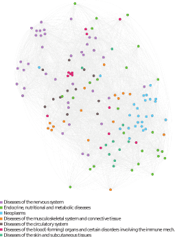
Figure 2: Cosine-similarity network among disease representations learnt by GSEM. Node colour indicates disease class. The plot has been produced via Gephi (Bastian et al., 2009) with ForceAtlas embedding.

7 Acknowledgements

We gratefully acknowledge the ERC-Consolidator Grant No. 724228 (LEMAN) for the support to MB and GG, the Vodafone Foundation supporting KV, IL and GG as part of the ongoing DreamLab/DRUGS project and the Imperial NIHR Biomedical Research Center for prospective clinical trials for the support to MB, KV, IL and GG.

AP and DG were supported in part by Biotechnology and Biological Sciences Research Council (BBSRC), grants BB/K004131/1, BB/F00964X/1 and BB/M025047/1 to AP, CONACYT Paraguay Grant INVG01-112 (14-INV-088) and PINV15-315 (14-INV-088), and NSF Advances in Bio Informatics grant 1660648.

FF was supported by the SNF Grant No. 200021E/176315.

References

- Ashburn and Thor [2004] Ted T Ashburn and Karl B Thor. Drug repositioning: Identifying and developing new uses for existing drugs. Nature Reviews Drug Discovery, 3(8):673–683, aug 2004.
- Bastian et al. [2009] Mathieu Bastian, Sebastien Heymann, and Mathieu Jacomy. Gephi: An open source software for exploring and manipulating networks. In International AAAI Conference on Weblogs and Social Media. Association for the Advancement of Artificial Intelligence, 2009.
- Berry et al. [2007] Michael W Berry, Murray Browne, Amy N Langville, V Paul Pauca, and Robert J Plemmons. Algorithms and applications for approximate nonnegative matrix factorization. Computational statistics & data analysis, 52(1):155–173, 2007.
- Boyd and Vandenberghe [2004] Stephen Boyd and Lieven Vandenberghe. Convex optimization. Cambridge university press, 2004.
- Bronstein et al. [2017] Michael M Bronstein, Joan Bruna, Yann LeCun, Arthur Szlam, and Pierre Vandergheynst. Geometric deep learning: going beyond euclidean data. IEEE Signal Processing Magazine, 34(4):18–42, 2017.
- Cáceres and Paccanaro [2019] Juan J Cáceres and Alberto Paccanaro. Disease gene prediction for molecularly uncharacterized diseases. PLoS computational biology, 15(7):e1007078, 2019.
- Caniza et al. [2015] Horacio Caniza, Alfonso E Romero, and Alberto Paccanaro. A network medicine approach to quantify distance between hereditary disease modules on the interactome. Scientific reports, 5:17658, 2015.
- Elhamifar [2016] Ehsan Elhamifar. High-rank matrix completion and clustering under self-expressive models. In Advances in Neural Information Processing Systems, pages 73–81, 2016.
- Fan and Chow [2017] Jicong Fan and Tommy WS Chow. Matrix completion by least-square, low-rank, and sparse self-representations. Pattern Recognition, 71:290–305, 2017.
- Gottlieb et al. [2011] Assaf Gottlieb, Gideon Y. Stein, Eytan Ruppin, and Roded Sharan. PREDICT: A method for inferring novel drug indications with application to personalized medicine. Molecular Systems Biology, 7(496):1–9, 2011.
- Hamilton et al. [2017] William L Hamilton, Rex Ying, and Jure Leskovec. Representation learning on graphs: Methods and applications. arXiv:1709.05584, 2017.
- Hamosh et al. [2004] A Hamosh, Alan F Scott, Joanna S Amberger, Carol A Bocchini, and Victor A McKusick. Online Mendelian Inheritance in Man (OMIM), a knowledgebase of human genes and genetic disorders. Nucleic Acids Research, 33(Database issue):D514–D517, dec 2004.
- Hinton [2018] Geoffrey Hinton. Deep learning—a technology with the potential to transform health care. Jama, 320(11):1101–1102, 2018.
- Kalofolias et al. [2014] Vassilis Kalofolias, Xavier Bresson, Michael Bronstein, and Pierre Vandergheynst. Matrix completion on graphs. arXiv:1408.1717, 2014.
- Kearfott and Walster [2000] R Baker Kearfott and G William Walster. On stopping criteria in verified nonlinear systems or optimization algorithms. ACM Transactions on Mathematical Software (TOMS), 26(3):373–389, 2000.
- Lee and Seung [1999] Daniel D Lee and H Sebastian Seung. Learning the parts of objects by non-negative matrix factorization. Nature, 401(6755):788, 1999.
- Lee and Seung [2001] Daniel D Lee and H Sebastian Seung. Algorithms for non-negative matrix factorization. In Advances in neural information processing systems, pages 556–562, 2001.
- Li and Ding [2006] Tao Li and Chris Ding. The relationships among various nonnegative matrix factorization methods for clustering. In Data Mining, 2006. ICDM’06. Sixth International Conference on, pages 362–371. IEEE, 2006.
- Luo et al. [2016] Huimin Luo, Jianxin Wang, Min Li, Junwei Luo, Xiaoqing Peng, Fang-Xiang Wu, and Yi Pan. Drug repositioning based on comprehensive similarity measures and Bi-Random walk algorithm. Bioinformatics, 32(17):2664–2671, sep 2016.
- Luo et al. [2018] Huimin Luo, Min Li, Shaokai Wang, Quan Liu, Yaohang Li, and Jianxin Wang. Computational drug repositioning using low-rank matrix approximation and randomized algorithms. Bioinformatics, 34(11):1904–1912, jun 2018.
- Ma et al. [2011] Hao Ma, Dengyong Zhou, Chao Liu, Michael R Lyu, and Irwin King. Recommender systems with social regularization. In Proceedings of the fourth ACM international conference on Web search and data mining, pages 287–296. ACM, 2011.
- Monti et al. [2017] Federico Monti, Michael Bronstein, and Xavier Bresson. Geometric matrix completion with recurrent multi-graph neural networks. In Advances in Neural Information Processing Systems, pages 3697–3707, 2017.
- Napolitano et al. [2013] Francesco Napolitano, Yan Zhao, Vânia M. Moreira, Roberto Tagliaferri, Juha Kere, Mauro D’Amato, and Dario Greco. Drug repositioning: A machine-learning approach through data integration. Journal of Cheminformatics, 5(6):1–9, 2013.
- Ng [2004] Andrew Y Ng. Feature selection, l 1 vs. l 2 regularization, and rotational invariance. In Proceedings of the twenty-first international conference on Machine learning, page 78. ACM, 2004.
- Pushpakom et al. [2018] Sudeep Pushpakom, Francesco Iorio, Patrick A. Eyers, K. Jane Escott, Shirley Hopper, Andrew Wells, Andrew Doig, Tim Guilliams, Joanna Latimer, Christine McNamee, Alan Norris, Philippe Sanseau, David Cavalla, and Munir Pirmohamed. Drug repurposing: progress, challenges and recommendations. Nature Reviews Drug Discovery, 18:41–58, oct 2018.
- Rudin [2019] Cynthia Rudin. Stop explaining black box machine learning models for high stakes decisions and use interpretable models instead. Nature Machine Intelligence, 1(5):206, 2019.
- Saito and Rehmsmeier [2015] Takaya Saito and Marc Rehmsmeier. The precision-recall plot is more informative than the ROC plot when evaluating binary classifiers on imbalanced datasets. PloS one, 10(3):e0118432, mar 2015.
- Van Driel et al. [2006] Marc A Van Driel, Jorn Bruggeman, Gert Vriend, Han G Brunner, and Jack AM Leunissen. A text-mining analysis of the human phenome. European journal of human genetics, 14(5):535, 2006.
- Wang and Elhamifar [2018] Yugang Wang and Ehsan Elhamifar. High rank matrix completion with side information. In Thirty-Second AAAI Conference on Artificial Intelligence, 2018.
- WHO [2016] WHO. International statistical classification of diseases and related health problems (10th Revision), 2016. URL https://icd.who.int/browse10/2016/en.
- Wishart et al. [2018] David S Wishart, Yannick D Feunang, An C Guo, Elvis J Lo, Ana Marcu, Jason R Grant, Tanvir Sajed, Daniel Johnson, Carin Li, Zinat Sayeeda, Nazanin Assempour, Ithayavani Iynkkaran, Yifeng Liu, Adam Maciejewski, Nicola Gale, Alex Wilson, Lucy Chin, Ryan Cummings, Diana Le, Allison Pon, Craig Knox, and Michael Wilson. DrugBank 5.0: a major update to the DrugBank database for 2018. Nucleic Acids Research, 46(D1):D1074–D1082, jan 2018.
- Zou and Hastie [2005] Hui Zou and Trevor Hastie. Regularization and variable selection via the elastic net. Journal of the royal statistical society: series B (statistical methodology), 67(2):301–320, 2005.