How to Pare a Pair: Topology Control and Pruning in Intertwined Complex Networks.

Abstract

Recent work on self-organized remodeling of vasculature in slime-mold, leaf venation systems and vessel systems in vertebrates has put forward a plethora of potential adaptation mechanisms. All these share the underlying hypothesis of a flow-driven machinery, meant to alter rudimentary vessel networks in order to optimize the system’s dissipation, flow uniformity, or more, with different versions of constraints. Nevertheless, the influence of environmental factors on the long-term adaptation dynamics as well as the networks structure and function have not been fully understood. Therefore, interwoven capillary systems such as found in the liver, kidney and pancreas, present a novel challenge and key opportunity regarding the field of coupled distribution networks. We here present an advanced version of the discrete Hu–Cai model, coupling two spatial networks in 3D. We show that spatial coupling of two flow-adapting networks can control the onset of topological complexity in concert with short-term flow fluctuations. We find that both fluctuation-induced and spatial coupling induced topology transitions undergo curve collapse obeying simple functional rescaling. Further, our approach results in an alternative form of Murray’s law, which incorporates local vessel interactions and flow interactions. This geometric law allows for the estimation of the model parameters in ideal Kirchhoff networks and respective experimentally acquired network skeletons.

I Introduction

Many recent studies on biological transportation networks have been focused on the hypothesis that vasculature is remodeled according to the flow-induced stress sensed by the cells making up the tissue le Noble et al. (2005). This self-organized process optimizes the structures for the task at hand , e.g. distributing oxygen and nutrients, getting rid of waste, carrying local secretion. The actual tissue response is dependent on the time-scales probed. On the one hand, short-term changes usually concern rapid vessel diameter changes in response to pressure fluctuations or medication. On the other hand, long-term effects e.g. due to metabolic changes may manifest in permanent diameter changes Hu et al. (2012), usually leaving the vessel structure with a trade-off between efficiency and redundancy Ronellenfitsch and Katifori (2019).
Particular focus has been directed to the long-term remodeling of the capillary plexus and other rudimentary transport systems in the early developmental stages of organisms, i.e. by studying complex signaling cascades involving growth factors like VEGF in vascular systems of mammals Risau (1997) or auxin in plants Dimitrov and Zucker (2006). Yet, the onset of refinement seems to be correlated with mechanical stresses (such as shear flow) as has been shown in a variety of model organisms from chicken embryo le Noble et al. (2005); Nguyen et al. (2006) and zebrafish Lenard et al. (2015) to leaves Roth-Nebelsick et al. (2001) and slime mold Tero et al. (2007).
Early theoretical approaches by Murray Murray (1926a, b) posited that diameter adaptation would minimize the overall power dissipation of the system. Following this ansatz of network optimization, many recent models are using global optimization schemes on expanded vessel networks. These models captured the phenomenon of link pruning involving random damage, flow fluctuations or rescaled volume costs and have been able to account for the trade-off of shunting and redundancies Bohn and Magnasco (2007); Katifori et al. (2010); Corson (2010). Further advances have been made in empirical studies of local vessel dynamics, e.g. blood vessel systems Pries et al. (1998, 2001); Secomb et al. (2013). Local adaptation dynamics were also effectively derived by minimizing various effective network costs via gradient descent methods Hu and Cai (2013); Chang and Roper (2019). It has further been shown that the outcomes of locally adapting networks are robust against variations of the initial topological structure Gräwer et al. (2015) and that plexus growth and correlated flow fluctuations can provide elaborate hierarchies Ronellenfitsch and Katifori (2016, 2019). Many of these effects may also be seen in continuous adaptation models in porous media Haskovec et al. (2015, 2016). It is interesting and important to note here that these adaptation mechanisms may leave certain fingerprints, e.g. in the form of allometric West et al. (1997) and geometric laws Sherman (1981).
These studies typically involve volume or metabolic constraints applied to abstract Kirchhoff networks. Yet they disregard the key characteristic common to all fluid transport systems: spatial embedding, which matters especially in the case of capillary systems as these directly interact via transport of metabolites with the surrounding tissue. These systems have to maintain a robust structure while being embedded in a possibly stiff tissue environment potentially perturbing the shear stress driven adaptation mechanism.
We here focus on the development and function of multicomponent flow networks, which influence each other based on their spatial architecture. Biologically speaking, these systems often consist primarily of blood vessels and a secondary entangled, interacting system as found for example in liver lobule Lautt (2007); Boyer (2013); Meyer et al. (2017); Morales-Navarrete et al. (2015), the kidney’s nephrons Shah et al. (2004); Serluca et al. (2002), the pancreas Magenheim et al. (2011); Villasenor and Cleaver (2012); Azizoglu et al. (2016) or the lymphatic system Planas-Paz and Lammert (2013). Additionally, we intend to include the phenomenon of one flow network being ‘caged’ by another complementary structure, e.g. capillaries embedded in bone marrow Sivaraj and Adams (2016).
In this work we study the adaptation of two coupled spatial networks according to an advanced version of the discrete Hu–Cai model Hu and Cai (2013) including Corson fluctuations Corson (2010). Each network is subject to flow driven and volume-constrained optimization on its own. Meanwhile we introduce the networks’ interaction in the form of a mutual repulsion or attraction of vessel surfaces. Repulsion will prevent them from touching directly by their otherwise flow driven radius expansion, introducing a competition of the two networks for the space they are embedded in. Alternatively, vessel surfaces could be be attracted towards each other, presenting a positive feedback towards maintaining intertwined structures. In combination with fluctuation induced redundancy, we find mutual repulsion to greatly reduce the networks relative loop density even when strong fluctuations are present. On the other hand we observe the emergence of a new sharp transition towards a loopy state when there is attraction between the two networks.
Unfortunately few metrics provide the means to fit or estimate the applied parameters of adaptation models for real systems, even though time-lapse experiments Lenard et al. (2015), counting pruning events and topology analysis on pruned structures Ronellenfitsch and Katifori (2019); Modes et al. (2016); Papadopoulos et al. (2018) allow for qualitative insights into the mechanism at hand for certain model organisms. Yet there has been no proposal to our knowledge to quantitatively acquire or fit the model parameters from real, pruned network structures. In particular, interwoven systems present a special challenge as typical experimental setups for a full 3D reconstruction involve invasive measures, i.e. sacrificing the specimen and preventing any long-term vessel observation. To tackle this problem we generalize an important scaling law, which has been discussed again recently in this context Akita et al. (2016): Murray’s Law. Our generalization enables us to reconstruct the model parameters with high fidelity for Kirchhoff networks solely from a given graph topology and it’s edge radii distribution (assuming the pruning process reached a stationary state). We find order of magnitude estimate for these parameters in experimentally acquired data sets of an interwoven system: sinusoids and canaliculi in the mouse’s liver acinus.
We begin our study in section II with a brief reminder of the hydrodynamical and network theoretical background on which we operate. Next we set up our model framework and its crucial components in detail. In section III we present the numerical evaluation of our model, in particular illuminating the cases of repulsive and attractive coupling between networks. In section IV we derive and test our generalized geometric laws on ideal Kirchhoff networks and on datasets of vessel networks provided by our collaborators. We then go on to discuss the implications and limits of our model framework in the concluding section V.

II Theoretical Framework

The following subsections are intended to provide the reader with the necessary background to proceed to the complex adaptation dynamics on ramified vascular networks that follow. Readers familiar with the general formalities should feel free to skip ahead to section II.3 where we discuss our general set up.
First we introduce the framework of Kirchhoff networks as these provide us with the mathematical tools needed to describe complex flow landscapes. Afterwards, we reintroduce the cost-function ansatz, the associated metabolic costs, and the chosen method of optimization which will render towards adaptation dynamics. Next, we discuss the intended hydrodynamic regime and the geometry of the intertwined system. We then extend our established framework by including fluctuation of the flow landscape as an essential tool to generate robust distribution networks. Finally, in the last subsection we introduce the relevant order parameters and metrics.

II.1 Fundamentals of linear networks

We model the biological vessel networks of interest as a composition of $m$ edges and $n$ vertices (branching points). Each edge carries a flux $f$ such that at any vertex the sum of all currents equal a nodal function $s$,

$$\sum_{e\in\operatorname{inc}(v)}f_{e}=s_{v}$$ (1)

where $\operatorname{inc}(n)$ indicates the set of edges incident to vertex $v$. We refer to $s$ as sink or source when $s$ is non-zero. Equation (1) is Kirchhoff’s current law, which represents mass conversation at every vertex. Further, in linear flow networks one may formulate the flux as a linear function, Ohm’s law, as:

$$f_{e}=c_{e}\Delta p_{e}$$ (2)

where $c_{e}$ is the conductivity of an edge and $\Delta p_{e}$ its respective potential gradient. One may thus characterize the flux in every vessel as a direct response to a gradient of potential energy, concentration, temperature etc. and have it scale linearly with the conductivity which incorporates the geometry and physical nature of the transport problem. The equation systems formulated in (1) and (2) may be bundled in vectorial notation as:

$$\boldsymbol{B}\cdot\boldsymbol{f}=\boldsymbol{s}$$ (3)

$$\boldsymbol{f}=\boldsymbol{C}\cdot\Delta\boldsymbol{p}$$ (4)

Here $\boldsymbol{B}$ designates the incidence matrix and $\boldsymbol{C}$ is a diagonal matrix with $c_{e}$ on the diagonal. Combining equations (3) and (4) one finds the transformation between the sinks/sources and the potentials as:

$$\boldsymbol{B}\cdot\boldsymbol{C}\cdot\Delta\boldsymbol{p}=\boldsymbol{s}$$ (5)

Unfortunately, this equation system is under-determined and accordingly seems to lack a unique solution for $\Delta\boldsymbol{p}$. Interestingly enough one may find a unique solution to the problem (5) by applying the Thomson principle Kelly et al. (1991); Grady and Polimeni (2010). Following the Thomson principle, one considers the system to be characterized by a cost function, i.e. the energy dissipation defined as $\sum_{e}f_{e}^{2}/\tilde{c}_{e}$, with positive coefficients $\tilde{c}_{e}\geq 0$. Further one may use this cost to formulate an optimization problem with Lagrange multipliers $p_{v}$ and the boundary conditions (1) such that:

$$\Gamma=\sum_{e}f_{e}^{2}/\tilde{c}_{e}+\sum_{v}p_{v}\left(s_{v}-\sum_{e^{\prime}\in\operatorname{inc}(v)}f_{e^{\prime}}\right)$$ (6)

The aim is to find the set of flows $f_{e}$ which minimize the system’s cost, $\Gamma$, with respect to the constraints given by the Kirchhoff current law. Doing so one will end up naturally with Ohm’s law, with the conductivities $c_{e}=\tilde{c}_{e}$ for the coefficients and the Lagrange parameters $p_{v}$ representing the nodal potentials. These $p_{v}$ define the potential gradients as $\Delta p_{e}=\left(p_{\omega(e)}-p_{\alpha(e)}\right)$, where $\alpha(e),\omega(e)$ designate the initial and final vertex of any edge $e$. This cost function ansatz enables one to find a unique solution for the potential differences $\Delta p$ in equation (5) as:

$$\Delta\boldsymbol{p}=\boldsymbol{C}^{-1/2}\left[\boldsymbol{B}\cdot\boldsymbol{C}^{1/2}\right]^{\dagger}\boldsymbol{s}$$ (7)

where $\left[\cdot\right]^{\dagger}$ designates the generalized inverse Penrose (1955). This solution represents the optimal potential landscape, which minimizes the overall power dissipation for a given landscape of conductivities and sinks Ben-Israel and Charnes (1963); Penrose (1956). Note that this formalism may be applied to any stationary transport process following the Thomson principle as well as random walks of particles on a lattice. This class of systems is often referred to as lumped systems or Kirchhoff networks, in analogy to simple electric circuits Desoer and Kuh (1969).

II.2 Cost function ansatz and optimization of biological networks

The concept of characterizing a transport network by a cost may readily be transferred to dynamic biological systems. The cells which are forming the walls of vascular networks for example, are able to respond and adapt to a given set of stimuli such as shear stress or hydrostatic pressure. This enables such systems to continuously change their own topology and edge conductivities in order to reach final refined structures. To capture this behavior one may formulate a cost for a vessel systems as proposed in Bohn and Magnasco (2007):

$$\Gamma=\sum_{e}\frac{f_{e}^{2}}{c_{e}}+ac_{e}^{\gamma}$$ (8)

where the first term is the power dissipation as before and the second a metabolic cost term $c_{e}^{\gamma}$, with proportionality factor $a$. This second term encapsulates the notion that a biological organism is constrained by the metabolic costs to deploy and sustain a vessel of a certain conductivity. The exponent $\gamma$ represents a degree of freedom to vary the relative importance of vessels of low or high conductivity.
The minimization of the function (8) is performed by finding the set of conductivities $c_{e}$ which minimizes (8) for a given boundary condition $\boldsymbol{s}$. Following the ansatz in Hu and Cai (2013) we may formulate our minimization in the form of temporal adaptation rules for each vessel, where each element reacts to a local stimulus, instead of a single global optimization procedure. To derive a local adaption dynamic we perform a gradient descent approach. This means we consider the temporal derivative $\Gamma$ as:

$$\frac{d\Gamma}{dt}=\sum_{j}\bigtriangledown_{c_{e}}\Gamma\cdot\partial_{t}c_{e}$$ (9)

We want to ensure $\frac{d\Gamma}{dt}\leq 0$ and therefore that $\Gamma$ converges towards a local minimum. To do so we may formulate the dynamical equations for $c_{e}$ as the negative gradient of $\Gamma$:

$$\partial_{t}c_{e}\propto-\bigtriangledown_{c_{e}}\Gamma=\left(\frac{f_{e}^{2}}{c_{e}^{2}}-a\gamma c_{e}^{\gamma-1}\right)$$ (10)

where we used the definition of $\Gamma$ in equation (8). The dynamics in equation (10) allow for a continuous local adaptation of the vessel’s state by consideration of its local flux, current conductivity and metabolic parameters $a,\gamma$. We extend this approach for interacting multilayer networks in a linear manner by adding up the metabolic cost of the individual systems involved and adding respective interaction terms. In our particular case we do so for two flow networks with:

$$\Gamma=\Gamma_{12}+\Gamma_{1}+\Gamma_{2}$$ (11)

where $\Gamma_{1}$, $\Gamma_{2}$ are given for each network by equation (8). The interaction term $\Gamma_{12}$ incorporates the geometrical nature of the system and encapsulates either a competition or symbiosis of the vessels of the two systems on a local basis as well. The exact nature of this interaction term as well as of the metabolic costs will be discussed in the next section in further detail, where we derive the dynamical systems in accordance with equation (10).

II.3 Modeling intertwined vessel systems

In this section we connect the results of the previous sections to the relevant hydrodynamics and discuss the nature of the exact biological flows problem. The direct applicability of equations (3), (4) to biological systems becomes clear when considering the Hagen–Poiseuille law Landau and Lifshits (1959) which describes the volume flow rate $f$ of a fluid of viscosity $\eta$ at low Reynold numbers through a tube of length $l$ and radius $r$ as:

$$f=\left(\frac{\pi r^{4}}{8\eta l}\right)\Delta p$$ (12)

This provides us with a conductivity $c=\frac{\pi r^{4}}{8\eta l}$ by direct comparison with Ohm’s law, with a fourth order dependency of the radius $r$. We will here focus on radial adaptation and consider the special case of $l_{i}=\text{const.}$ for all vessels in either network. Hence, using equations (8), (12) we may rewrite the cost ansatz in (11) as:

$$\Gamma= \Gamma_{12}+\left(\frac{\pi}{8\eta_{1}l_{1}}\right)\left[\sum_{e_{1}}r_{e_{1}}^{4}\Delta p_{e_{1}}^{2}+a_{1}r_{e_{1}}^{4\gamma_{1}}\right]$$

$$+\left(\frac{\pi}{8\eta_{2}l_{2}}\right)\left[\sum_{e_{2}}r_{e_{2}}^{4}\Delta p_{e_{2}}^{2}+a_{2}r_{e_{2}}^{4\gamma_{2}}\right]$$ (13)

From here on we use the indices $i\in\{1,2\}$ for the two networks. Further, we only consider the specific case $\gamma_{i}=0.5$, which relates the metabolic cost directly towards volume for each vessel. Performing a minimization of the cost (13) at this point, without considering any interactions $\Gamma_{12}$, would result in each network to independently become dissipation minimized, constrained by its overall volume. We thus turn our attention to the interaction term $\Gamma_{12}$.

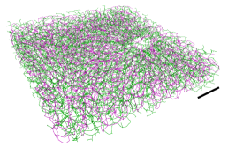
(a)

(b)

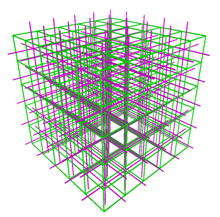
(c)

Figure 1: LABEL:sub@fig:real_network  Biological intertwined structures: segment of bile canaliculi (green) and sinusoids (magenta) in the mouse’s liver acinus (presented as network skeletons, see also Morales-Navarrete et al. (2015) )), scale bar is $200\ \mu m$. Modeling two interacting networks and 3D network skeletons of triply-periodic minimal surfaces for initial plexi: LABEL:sub@fig:model_a  (Cubic) unit cell and indication of spatial constraint for tube surfaces. LABEL:sub@fig:model_b  Complementary cubic lattices.

In order to model interacting networks such as those found in the liver lobule (see Figure 1a) we define a multilayer network consisting of two intertwined, yet spatially separate objects each consisting of edges $e_{i}$, with designated vessel radii $r_{e_{i}}$ see Figure 1b and 1c. Each edge in either network is affiliated with the set of closest adjacent edges of the other respective network. As all theses edges are simply tubes in our model, we define the distance between affiliated tube surfaces to be,

$$\Delta r_{e_{1}e_{2}}=L-\left(r_{e_{1}}+r_{e_{2}}\right)$$ (14)

where $L$ is the initial distance of the abstract network skeletons (equal to distance in case of simultaneously vanishing radii). To model a system of blood vessels entangled with a secondary, secreting vessel network, we postulate that the respective tube surfaces must not fuse or touch directly, i.e. $\Delta r_{e_{1}e_{2}}\geq 0$. Subsequently, we construct the interaction term $\Gamma_{12}$ for the combined system as a power of the relative distance $\Delta r_{e_{1}e_{2}}$:

$$\Gamma_{12} =\frac{b}{2}\sum_{e_{1}e_{2}}F_{e_{1}e_{2}}\Delta r_{e_{1}e_{2}}^{\varepsilon}$$ (15)

$$\text{ with }F_{e_{1}e_{2}} =\begin{cases}1&\text{if edges }e_{1}\text{ and }e_{2}\text{ affiliated}\\ 0&\text{else}\end{cases}$$ (16)

with positive coefficient $b\geq 0$ and exponent $\varepsilon\in\mathbb{R}$ allowing us to switch between a repulsive or attractive behavior of the interaction, see section II.4, resembling either the competition for space or a mechanism to increase mutual contact. We have therefore arrived at the total cost function for the system:

$$\Gamma= \frac{b}{2}\sum_{e_{1}e_{2}}F_{e_{1}e_{2}}\Delta r_{e_{1}e_{2}}^{\varepsilon}$$

$$+\left(\frac{\pi}{8\eta_{1}l_{1}}\right)\left[\sum_{e_{1}}r_{e_{1}}^{4}\Delta p_{e_{1}}^{2}+a_{1}r_{e_{1}}^{2}\right]$$

$$+\left(\frac{\pi}{8\eta_{2}l_{2}}\right)\left[\sum_{e_{2}}r_{e_{2}}^{4}\Delta p_{e_{2}}^{2}+a_{2}r_{e_{2}}^{2}\right]$$ (17)

which we may now use to derive the dynamical system via gradient descent.

II.4 Adaptation dynamics of intertwined vessel systems

In this section we discuss in detail the dynamical systems we intend to construct via the gradient descent approach on the basis of the cost function shown in equation (17). Calculating the gradient we acquire the equations of motion for each network as:

$$\partial_{t}r_{e_{1}}\propto \left[\Delta p^{2}_{e_{1}}r_{e_{1}}^{2}-\frac{a_{1}}{2}\right]r_{e_{1}}$$

$$+\frac{b\eta_{1}l_{1}\varepsilon}{\pi}\sum_{e_{2}}F_{e_{1}e_{2}}\Delta r_{e_{1}e_{2}}^{\varepsilon-1}$$ (18)

$$\partial_{t}r_{e_{2}}\propto \left[\Delta p^{2}_{e_{2}}r_{e_{2}}^{2}-\frac{a_{2}}{2}\right]r_{e_{2}}$$

$$+\frac{b\eta_{2}l_{2}\varepsilon}{\pi}\sum_{e_{1}}F_{e_{1}e_{2}}\Delta r_{e_{1}e_{2}}^{\varepsilon-1}$$ (19)

The details of the derivation are given in the supplementary material A. It may be noted here that the terms $\Delta p_{i}^{2}r_{i}^{2}$ correspond to the wall shear stress exerted, manifesting itself in a positive growth feedback. The negative terms $\frac{a_{i}}{2}$ relate towards the metabolic cost. This term imposes effectively a volume penalty on the system as growing vessels generate an increased negative feedback. The interaction term reacts to the relative vessel distance $\Delta r$ and imposes a feedback connected to the local neighborhood of each vessel which can be either positive (attractive coupling) or negative (repulsive coupling) depending on the choice of $\varepsilon$.
In order to perform a numerical evaluation of the resulting ODE system we define a unit system and non-dimensional parameters as follows: the radii and edge lengths in units of the grid distance $r_{e_{i}}=Lr_{e_{i}}^{*}$ , $l_{i}=Ll_{i}^{*}$, the nodal in and outflow $s_{v_{i}}=\mu_{i}s_{v_{i}}^{*}$, the conductivity $c_{e_{i}}=\eta_{i}^{-1}L^{3}c_{e_{i}}^{*}$ and hence pressure $\Delta p_{e_{i}}=\frac{\mu_{i}\eta_{i}}{L^{3}}\Delta p_{e_{i}}^{*}$ and the networks’ edge surface distance $\Delta r_{{e_{1}e_{2}^{\prime}}}^{\varepsilon-1}=L^{\varepsilon-1}\Delta r_{e_{1}e_{2}}^{*\varepsilon-1}$. We define the time scale via the volume flow rates in the primal network as $t=\frac{L^{3}}{\mu_{1}}t^{*}$. Given positive proportionality constants $\chi_{i}\geq 0$ in the equations (18), (19), we define the effective temporal response parameters in either network as ${\lambda_{0}^{i}=\frac{\chi_{1}L^{3}}{\mu_{1}}\left(\frac{\mu_{i}\eta_{i}}{L^{2}}\right)^{2}}$. Further we define the effective network couplings ${\lambda_{1}^{i}=\frac{b|\varepsilon|L^{3+\varepsilon}}{\pi\eta_{i}\mu_{i}^{2}}}$ and the effective volume penalties ${\lambda_{2}^{i}=\frac{a_{i}}{2}\left(\frac{L^{2}}{\mu_{i}\eta_{i}}\right)^{2}}$. We introduce an effective coupling $g^{*}_{e_{i}}$ term as

$$g_{e_{1}}^{*}=\operatorname{sgn}(\varepsilon)l_{i}^{*}\sum_{e_{2}}F_{e_{1}e_{2}}\Delta r_{e_{1}e_{2}}^{*\varepsilon-1}$$ (20)

$$g_{e_{2}}^{*}=\operatorname{sgn}(\varepsilon)l_{i}^{*}\sum_{e_{1}}F_{e_{1}e_{2}}\Delta r_{e_{1}e_{2}}^{*\varepsilon-1}$$ (21)

using the sign function $\operatorname{sgn}(\varepsilon)$. We thus arrive at the dimensionless form of the dynamical equations for each network:

$$\partial_{t^{*}}r_{e_{i}}^{*}=\lambda_{0}^{i}\left(\Delta p_{e_{i}}^{*2}r_{e_{i}}^{*3}-\lambda_{2}^{i}r_{e_{i}}^{*}+\lambda_{1}^{i}g_{e_{i}}^{*}\right)$$ (22)

The coupling $g_{e_{i}}^{*}$ changes its qualitative behavior with variation of the exponent $\varepsilon$. We will consider the cases of an attractive coupling $\varepsilon>1$ and a repulsive coupling $\varepsilon<0$, see Figure 2. We will further discuss the trivial case of an uncoupled system $\varepsilon=0$ (for which $\lambda_{1}=0$) for direct comparison with the Hu–Cai model. Note that $\varepsilon=1$ will result in a constant $g_{e_{i}}^{*}$ corresponding to a positive constant background stimuli, as proposed by Ronellenfitsch and Katifori (2016). The case $0<\varepsilon<1$ results in a diverging attraction for nearby vessels, while it basically drops out for $\Delta r_{e_{1}e_{2}}\longrightarrow 1$. These numerically and heuristically unfavorable cases of $0<\varepsilon<1$ as well as the linear case $\varepsilon=1$ will be neglected hereafter.

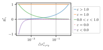
Figure 2: The effective behavior of the coupling term $g_{e_{i}}^{*}$ changes with variation of the exponent $\varepsilon$ . Function values of $g_{e_{i}}^{*}$ are presented here dependent on the distance of a single arbitrary vessel pairing, curves normalized for comparison.

II.5 Incorporating flow fluctuations: Noisy, uncorrelated sink patterns

Next we assume the adaptation of the vascular networks depends on an averaged potential landscape instead of instantaneous configurations, which are bound to occur in real systems due to short-term metabolic changes or vessel blocking/damage. In other words, we assume a constant vessel radius between two adaptation events, while the flow rates change throughout the system due to changes in the sinks’ magnitude, enabling us to substitute ${\Delta p_{e}^{2}\rightarrow\left<\Delta p_{e}^{2}\right>}$ in equation (22). We thus implicitly assume a time-scale separation between the radii adaptation (long-time changes, not to be confused with short term contraction/dilation) and changes of hydrostatic pressure. We define fluctuations in accordance to the Corson model Corson (2010). Subsequently, we will only consider $\boldsymbol{s}$-configurations in which there exists one source-node (here $v_{\text{source}}=0$, $s_{0}=-\sum_{v>0}s_{v}$) and all other nodes are randomly initialized sinks with the following characteristics:

$$\left<s_{v}\right>=\mu_{v}\text{ with }v>0$$ (23)

$$\left<s_{v}s_{w}\right>=\rho_{vw}\sigma_{v}\sigma_{w}+\mu_{v}\mu_{w}\text{ with }v,w>0$$ (24)

We assume the fluctuations are uncorrelated and follow the same probability distribution. We set for the mean $\mu_{v}=\mu$ , standard deviation $\sigma_{w}=\sigma$, and correlation coefficient $\rho_{vw}=\delta_{vw}$. We may subsequently calculate the average squared pressure:

$$\left<\Delta p_{e}^{2}\right>=\mu^{2}\phi_{e}+\sigma^{2}\delta\phi_{e}$$ (25)

where the function $\phi_{e}$ describes the squared pressure in the case of a constant source-sink landscape in the absence of any variance $\sigma^{2}$. Further, the function $\delta\phi_{e}$ describes the pressure perturbation caused by fluctuations with variation $\sigma^{2}$ in analogy to the Hu–Cai models heuristic fluctuation ansatz Hu and Cai (2013). For the full derivation of equation (25) and the detailed computation of $\phi_{e}$, $\delta\phi_{e}$ see supplementary material B. Using this approach we prevent shunting and the generation of spanning trees, which is caused by the typical ‘single source/multiple sinks’ setting. Further, using this ansatz one also prevents accidentally partitioning the graph which can happen when realizing the sink-source configurations one by one Ronellenfitsch and Katifori (2019).
We find this ansatz in particular fitting to model the liver lobule system, as sinusoids are fenestrated structures (meaning the vessel wall is perforated). Additionally, bile and water is frequently secreted by hepatocytes (cells forming the bulk of the tissue and the basic metabolic unit in the liver) into bile canaliculi. On the other hand, one may argue that the fluid leak in the sinusoidal system is negligible in comparison to the overall throughput rate, and an additional distinguished sink would have to be placed at the opposing end of the plexus, extracting the majority of fluid. Here we neglect this factor as one major sink would merely generate one (or a small number of) distinguished large vessel(s), without any further impact on the topological complexity of the rest of the networks.
We incorporate these flow fluctuations with an effective fluctuation strength ${\lambda_{3}^{i}=\frac{\sigma_{i}^{2}}{\mu_{i}^{2}}}$ in equation (22) :

$$\partial_{t^{*}}r_{e_{i}}^{*}=\lambda_{0}^{i}\left(\left(\phi_{e_{i}}^{*}+\lambda_{3}^{i}\delta\phi_{e_{i}}^{*}\right)r_{e_{i}}^{*3}-\lambda_{2}^{i}r_{e_{i}}^{*}+\lambda_{1}g_{e_{i}}^{*}\right)$$ (26)

Thereby $\lambda_{3}^{i}$ scales the strength of pressure perturbations, which effectively impose an increase in the wall shear stress term in equation (26).

II.6 Order parameters for network remodeling

In order to quantify the topological changes occurring in an adapting system we monitor the relative cycle density as an indicator of redundancy. Loosely, one may identify the number of cycles in a network in the following simple way: If we assume that the network’s representing simple graph is one connected component of $n$ vertices and $m$ edges, then we only need $n-1$ edges to connect every vertex into a spanning tree without a single cycle, while each additional edge added from here on will form a cycle. Thus the total amount of such cycles in a network $z$, is the number of excess edges from the total number of edges:

$$z=m-\left(n-1\right)$$ (27)

Strictly speaking, $z$ is the amount of independent cycles (also referred to as nullity) and may be calculated for any simple multicomponent graph Whitney (1932). We use this metric in the following way: We solve the dynamical systems (26) until the networks reach a stationary state. The initial graph structure this process starts from is called a plexus and represents in biological terms the rudimentary vessel network which is formed before perfusion sets in. During this optimization we mark edges whose radius falls below a critical threshold $r^{*}_{c}$. These edges are no longer updated and are considered to have a radius of virtually zero (though for computational reasons they are here set to $r^{*}_{c}=10^{-21}$). We call such edges ’pruned’ which corresponds to the biological phenomenon of having a vessel degenerate and collapse. Then we remove all pruned edges and disconnected vertices from the networks and calculate the remaining number of cycles according to equation (27). We then define the relative nullity of an equilibrated network,

$$\varrho=\frac{m-n+1}{z_{0}}$$ (28)

as an order parameter, where $z_{0}$ is the initial number of independent loops before adaptation. Hence $\varrho=0$ corresponds to a treelike network while $\varrho>0$ captures the relative amount of redundancy in comparison to the initial plexus.

III Numerical evaluation of the model framework

In this section we present the simulation results acquired by solving the dynamical system (26) numerically until the system reaches a stationary state. Of particular interest is the final network’s topology, i.e. its relative reticulation characterized by the order parameter $\varrho$. We study in detail the dependence of $\varrho$ on the coupling $\lambda_{1}$, the volume penalty $\lambda_{2}$, and the fluctuation rate $\lambda_{3}$. Primary focus lies on the interplay of coupling and fluctuation and how the underlying three dimensional lattice topology affects the remodeling process. All diagrams shown represent the results for one of the two intertwined networks; the results are symmetric for the other network due to a symmetric choice of the effective parameters $\lambda^{i}_{1}$, $\lambda^{i}_{2}$ and $\lambda^{i}_{3}$, see Appendix C for further details.
As underlying graph topology for the initial state networks we take the graph skeletons of the triply-periodic minimal surfaces P (‘dual’ simple cubic, see Figure 1c), D (‘dual’ diamond cubic) and G (‘dual’ Laves) Góźdź and Hołyst (1996). These systems present highly symmetric and complementary space filling graphs and enable us to construct well defined intertwined networks with clear local edge affiliations. The initial edge radii are chosen randomly. We set the fluctuation rates identical $\lambda_{3}^{1}=\lambda_{3}^{2}$ as well as the coupling strength $\lambda_{1}^{1}=\lambda_{1}^{2}$. We did not find any qualitative differences in our results among different intertwined topologies. We thus present here the results for the simplest starting topology, the intertwined cubic lattices.

III.1 Fluctuation induced nullity transitions independent of volume penalty and topology

First, we test the original Hu–Cai model in combination with Corson’s fluctuation approach, i.e. the uncoupled case of $\varepsilon=0$ for three dimensional lattices. We do so for two reasons: First, to confirm the robustness of the adaptation mechanic for a plexus represented by non-planar graphs in a similar manner to Gräwer et al. (2015). Second, to confirm the independence of the fluctuation-induced nullity transition from the volume penalty $\lambda_{2}$, as indicated in Hu and Cai (2013). To do so, we calculate the adaptation with a single corner source node (sinks otherwise) for a systematic scan of $\lambda_{2}$ and $\lambda_{3}$ (see Figure 3).
Indeed, we recover the transition from tree-like configurations for $\lambda_{3}\leq 1$ (Figure 3a) towards states exhibiting fluctuation induced loops for large $\lambda_{3}$ (Figure 3b). The emerging transition is of logarithmic nature, effectively saturating for $\lambda_{3}\approx 10^{4}$. In particular, we confirm that only an increase in the fluctuation ratio, $\lambda_{3}$, results in an increase in the nullity (Figure 3c). The continuous transition observed is independent of the system’s effective volume penalty $\lambda_{2}$ (Figure 3d). Note however, that the parameter $\lambda_{2}$ influence the final vessel diameter as well as the time scales for reaching the stationary state (as does the system size if the number of identical sinks scales with system size). Further, we confirm that the adaptation mechanism reproduces the qualitative network topologies in three dimensional lattices as found before in planar graphs. From here we turn our attention to the fluctuation induced transition in comparison to the new spatial coupling.

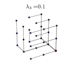
(a)

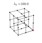
(b)

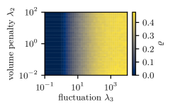
(c)

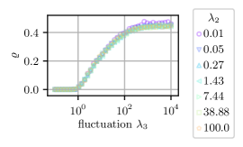
(d)

Figure 3: Stationary network configurations for $\lambda_{2}=1$. The edge thickness is representative for the relative tube radius $\rho$. Sinks are marked as blue dots, the source as large red circle. LABEL:sub@fig:prune_1  Tree-like for $\lambda_{3}=0.1$ LABEL:sub@fig:prune_3  Fluctuation induced loops for $\lambda_{3}=100$. LABEL:sub@fig:scale_a + LABEL:sub@fig:scale_b  Uncoupled adapting networks display continuous, logarithmic $\lambda_{2}$-independent nullity $\varrho$ transitions ($\lambda_{1}=0$, cubic lattice, $n=216$ and $m=540$).

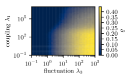
(a)

(b)

(c)

(d)

(e)

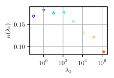
(f)

Figure 4: Nullity $\varrho$ transitions and state diagram for repulsively coupled networks ($\varepsilon=-1)$: LABEL:sub@fig:bilayer_nullity_a_rep Coupling vs fluctuation, $\left(\lambda_{1},\lambda_{3}\right)$-diagram with nullity $\varrho$ color map. LABEL:sub@fig:bilayer_nullity_b_rep Coupling $\lambda_{1}$ induced nullity breakdown for varying fluctuation $\lambda_{3}$. LABEL:sub@fig:bilayer_nullity_c_rep Fluctuation $\lambda_{3}$ induced nullity onset for varying coupling $\lambda_{1}$ LABEL:sub@fig:bilayer_nullity_d_rep Critical $\lambda_{3}$ for onset of nullity transition for $\lambda_{1}$ variation and extrapolated saturation of nullity transition. LABEL:sub@fig:bilayer_nullity_e_rep Single curve collapse near fluctuation induced nullity onset $\lambda_{c}$ and scaled nullity $\varrho/\kappa(\lambda_{3})$. We find the transition to be approximated by ${\varrho\left(\lambda_{1},\lambda_{3}\right)\approx\kappa\left(\lambda_{1}\right)\left(\log_{10}\left(\frac{\lambda_{3}-\lambda_{c}}{\lambda_{c}}\right)-1\right)}$ LABEL:sub@fig:bilayer_nullity_f_rep $\kappa\left(\lambda_{1}\right)$ dependency derived from linear interpolation of rescaled transition curves.

III.2 Repulsive coupling shifts and rescales fluctuation induced nullity transition

To consider the novel, spatially coupled cases, we systematically scan the effective network coupling and flow-fluctuation parameters. In this section we will focus on the case of repulsive interactions, i.e. setting the coupling exponent to $\varepsilon=-1$. Of particular interest is the influence of the negative feedback this interaction introduces to the dynamical system (26).
First, we see the fluctuation-induced nullity transition (as observed for the uncoupled system) to be preserved for weak couplings, $\lambda_{1}<10^{4}$. The full state diagram though (Figure 4a) shows that the system’s nullity may be influenced above that threshold not only by the rate of fluctuations $\lambda_{3}$, but also by the mutual repulsion of the two networks. Figure 4b shows the corresponding $\lambda_{1}$ induced breakdown, displaying the possibility to nullify any reticulated structures by increasing the repulsive coupling strength in the system. Nevertheless, it seems that the influence of the repulsion is weaker in comparison, needing coupling parameters to be orders of magnitudes larger than the fluctuation rates. On the other hand, we also find the fluctuation-induced nullity onset to be continuous, as it was for the uncoupled system. Starting from a tree-like state at small fluctuations and increasing monotonically in a logarithmic manner beyond a critical $\lambda_{3}\geq\lambda_{c}$ (Figure 4c) we have the $\varrho$-trajectory eventually saturating for large fluctuation rates $\lambda_{3}>10^{3}$ towards a maximal nullity $\varrho_{\text{max}}$. This leaves the network in a reticulated state, still displaying a visible vessel hierarchy towards the source. We can recover almost tree-like network states for increased repulsion rates $\lambda_{1}$, even losing the typical vessel hierarchy towards the source, see Figure 5. This increase in $\lambda_{1}$ further shifts the onset of nullity. To quantify these shifts we acquire the critical $\lambda_{c}$ by identifying the departure from zero in Figure 4c. The critical point $\lambda_{c}$ seems to monotonically increase with the coupling parameter $\lambda_{1}$. Following up on this observation we extrapolated the onset of saturation in Figure 4c by means of sigmoidal fits. The shifts of these indicators are shown in Figure 4d, displaying a general increase of both the critical value and the saturation for increasing $\lambda_{1}$. Using the acquired critical values $\lambda_{c}$ we rescale the trajectories of Figure 4c between the onset of the nullity transition and its saturation, as shown in Figure 4e. Introducing the reduced fluctuation parameter $\frac{\lambda_{3}-\lambda_{c}}{\lambda_{c}}$ we find the trajectories to collapse on a single master curve, following a trivial logarithmic law as:

$$\varrho\left(\lambda_{1},\lambda_{3}\right)\approx\kappa\left(\lambda_{1}\right)\left(\log_{10}\left(\frac{\lambda_{3}-\lambda_{c}}{\lambda_{c}}\right)-1\right)$$ (29)

with the coupling dependent scale $\kappa$ acquired by interpolation of the data by equation (29). We find $\kappa$ to be a decreasing function the coupling $\lambda_{1}$ as shown in Figure 4f. This shows that the nullity breakdown and shift can be tuned for any given fluctuation rate by the coupling alone. Further, the negative feedback (caused by the repulsion of the two networks) does not cause any shunting (i.e. collapse and disconnection of large sections of the networks) whatsoever.
For all simulations shown we set the response ${\lambda^{1}_{0}=\lambda_{0}^{2}=10^{-4}}$, and volume penalty ${\lambda^{1}_{2}=\lambda^{2}_{2}=10^{6}}$ (providing reasonable computation times for reaching stationary states and preventing the problem from becoming too stiff). The initial edge radii are chosen randomly and are subsequently continuously monitored to fulfill:

$$0<r^{*}_{e}+r^{*}_{e^{\prime}}<1$$ (30)

in order to prevent negative radii, or radii combinations corresponding to intersections.

Figure 5: Stationary network configurations for $\lambda_{2}=10^{6}$. The edge thickness is representative of the relative tube radius $r^{*}$. Sinks are marked as blue dots, the source as a large red circle. Repulsive coupling causes nullity breakdown and overall reduction in edge thickness leading to the disappearance of the usual vessel hierarchy.

III.3 Attractive coupling induces a new nullity transition, fully recovering initial plexus

We now consider intertwined networks with an attractive spatial coupling. We initialize the system with a positive coupling exponent, $\varepsilon=3$. We are particularly interested how the positive feedback this interaction introduces to the dynamical system (26) interacts and compares with the fluctuation induced nullity transition.
Indeed, the increased positive feedback from $\lambda_{1}$ leads to a significant increase in the system’s redundancy, as can be seen in Figure 6. In Figure 7 we show the resulting nullity state diagrams and transition curves for a systematic scan the couplings and fluctuation rates. For increasing coupling strength $\lambda_{1}$ we see the emergence of a new nullity transition for $\lambda_{1}>\lambda_{c}$. This transition recovers virtually the entire initial plexus for $\lambda_{1}\rightarrow 10^{4}$ (Figure 7b). Furthermore, this transition is significantly sharper than the fluctuation-induced case as it does not occur on a logarithmic scale. Any increase in fluctuations, $\lambda_{3}$, generates positive offset of the nullity curve (Figure 7b) indicating a constructive superposition of the mechanisms at hand. Yet, the trajectory’s general form seems well preserved, while the saturation level is reduced for increased $\lambda_{3}$. Once again we determine the transition’s onset and saturation regime, see Figure 7d. To do so for the onset, we calculate the trajectories’ root of the onset after subtracting the trajectories’ offset. The saturation regime is extrapolated via a sigmoidal fit. As in the previous section we are able collapse the trajectories onto a single master curve(Figure 7e) by following a trivial linear law :

$$\varrho\left(\lambda_{1},\lambda_{3}\right)\approx\kappa\left(\lambda_{3}\right)\left(\frac{\lambda_{1}-\lambda_{c}}{\lambda_{c}}\right)+\varrho_{0}\left(\lambda_{3}\right)$$ (31)

with rescaled x-axis $\frac{\lambda_{1}-\lambda_{c}}{\lambda_{c}}$. The $\lambda_{3}$ dependency of the respective scaling parameters are shown in Figure 7f. We note here that these curves are slightly different from the complementary network in the case of cubic lattice topology as they are considerably more spread out, see the supplementary material C for details. This phenomenon does seem to be topology dependent, as is not present in the case of Lave-graphs or diamond lattices. The fluctuation induced nullity transition on the other hand is in some sense perturbed beyond the $\lambda_{1}$ transition, see Figure 7c. It seems an underlying competition of mechanisms is observable for large $\lambda_{3}$ as the level of saturation is reduced, as can be directly seen in the scale factor $\kappa$, see Figure 7f. Nevertheless, this interplay between different positive feedback mechanisms creates multiple nullity states, see Figure 7a, tuning the structures between spanning trees, partially reticulated and fully recovered plexus.
For all simulations we set the response $\lambda_{0}^{i}=10^{-4}$, and volume penalty $\lambda_{2}^{i}=10^{6}$ as in the previous section. The parameter $\lambda_{3}$ is only considered here for $\lambda_{3}<300$ as affiliated edge pairs will violate the contact condition (30) beyond this range.

Figure 6: Stationary network configurations for $\lambda_{2}=10^{6}$. The edge thickness is representative for the relative tube radius $r^{*}$. Sinks are marked as blue dots, the source as a large red circle. Attractive coupling sets another local positive feedback which fixes overall nullity to the point of total plexus recovery.

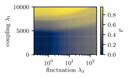
(a)

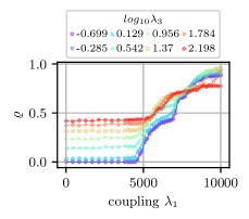
(b)

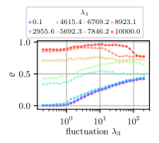
(c)

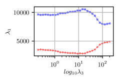
(d)

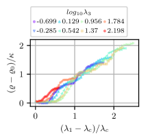
(e)

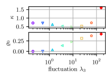
(f)

Figure 7: Nullity $\varrho$ transitions and state diagram for attractively coupled networks ($\varepsilon=3)$: LABEL:sub@fig:bilayer_nullity_a_att Coupling vs fluctuation, $\left(\lambda_{1},\lambda_{3}\right)$-diagram for nullity $\varrho$ color map. LABEL:sub@fig:bilayer_nullity_b_att Coupling $\lambda_{1}$ induced nullity transition for varying fluctuation $\lambda_{3}$. LABEL:sub@fig:bilayer_nullity_c_att Fluctuation $\lambda_{3}$ induced nullity transition for varying coupling $\lambda_{1}$. LABEL:sub@fig:bilayer_nullity_d_att Critical $\lambda_{1}$ for onset of nullity transition for $\lambda_{3}$ variation and extrapolated saturation of nullity transition. LABEL:sub@fig:bilayer_nullity_e_att Single curve collapse near coupling induced nullity onset $\lambda_{c}$ and scaled nullity $(\varrho-\varrho_{0}(\lambda_{3}))/\kappa(\lambda_{3})$. We find the transition to be approximated by $\varrho\left(\lambda_{1},\lambda_{3}\right)\approx\kappa\left(\lambda_{3}\right)\frac{\lambda_{1}-\lambda_{c}}{\lambda_{c}}+\varrho_{0}$ LABEL:sub@fig:bilayer_nullity_f_att $\kappa$ and $\varrho_{0}$ dependency derived from linear interpolation of rescaled curves.

IV Generalizing Murray’s law

Our model of spatial coupling also points to a new form of geometric law at vessel branchings. Recall Murray’s Law, which connects the radii $r_{0}$ of a parent vessel splitting into at least two child branches with radii $r_{1}$, $r_{2}$ as:

$$r_{0}^{\alpha}=r_{1}^{\alpha}+r_{2}^{\alpha}$$ (32)

In the original formulation an exponent of ${\alpha=3}$ was predicted as the outcome of a cost optimization process Murray (1926a) which relates directly to the dissipation-volume minimization procedure discussed in section II.2. Further, rescaled cost models Bohn and Magnasco (2007) which consider cost variations via an exponent ${c_{e}\rightarrow c_{e}^{\gamma}}$ suggest

$$\alpha=2\left(\gamma+1\right)$$ (33)

while discarding flow fluctuations. We illustrate here the problems one encounters when testing these power laws for real intertwined structures such as sinusoids and bile canaliculi in the mammalian liver. Further, we introduce a new generalized form of Murray’s Law which takes into account fluctuations as well as geometric coupling. We then use this new form to estimate the interaction parameters of the real system heretofore inaccessible to experimental investigation.
The datasets were acquired from collaborators at the MPI-CBG in the following way: Mouse livers from adult mice were fixed by trans-cardial perfusion, sectioned into 100 mm serial slices, optically cleared and immunostained, as described in Morales-Navarrete et al. (2015). To visualize the different tissue components, the tissue sections were stained for nuclei (DAPI), cell borders (Phalloidin), bile canaliculi network (CD13), and the extracellular matrix (ECM, fibronectin and laminin) facing the sinusoidal network Morales-Navarrete et al. (2019). High-resolution images of the liver lobule (Central vein – portal vein axis) were acquired by using confocal microscopy with a 63x/1.3 objective ($0.3\ \mu m$ voxel size). Finally, the resulting images were segmented and network skeletons calculated with the Motion Tracking software as described in Morales-Navarrete et al. (2015) and Morales-Navarrete et al. (2016).

IV.1 Classical Murray’s Law inadequate for reticulated, intertwined vessel structures of the liver lobule

We test Murray’s Law for the network skeletons of the sinusoids and bile canaliculi in the liver lobule by fitting the exponent $\alpha$ in equation (32) for every branching of degree three (Y-branching). There is significant deviation from the predicted exponent $\alpha=3$ (Figure 8).

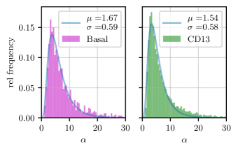
Figure 8: Exponent distributions found for Murray’s Law (32) and respective log-normal fits: Sinusoidal systems (basal marker) with mode $\alpha=e^{\mu-\sigma^{2}}\approx 3.75$ and bile canaliculi systems (cd13 marker) with mode $\alpha=e^{\mu-\sigma^{2}}\approx 3.33$.

The modes of the acquired, log-normally distributed fit exponents are $\alpha\approx 3.75$ for sinusoids and for bile canaliculi $\alpha\approx 3.33$. As capillary systems were already known to defy the cubic relationship Sherman (1981), we suspect this mismatch to be correlated with the reticulated nature of these network types. Further, one expects other mechanisms than mere dissipation-volume minimization will be involved, making these deviations not well described by the cost exponent $\gamma$ alone. Indeed, in accordance to equation (33) one would deduce $\gamma<1$ for the given liver lobule datasets which is in direct contradiction with the rescaled cost model Bohn and Magnasco (2007), which predicts an exponent $\gamma$-induced nullity transition only for $\gamma\geq 1$. On the other hand this could potentially be circumvented if fluctuation-induced loops are considered as well Katifori et al. (2010); Corson (2010). However, to our knowledge it has not yet been discussed how such fluctuations alter Murray’ Law.
We deduce from our pruning model a new set of coefficients, $a_{e}$, which are dependent on their corresponding edge’s neighborhood and the respective coupling strength, as well as the global structure of sinks and sources (which were assumed to be uncorrelated and identically distributed). This procedure greatly alters the form of equation (32) and we derive a new geometric law derived from the steady-states of the ODEs in (26). We recover the cubic exponent of the original model with new coefficient corrections that depend on the strength of fluctuations and spatial coupling:

$$\sum_{e}a_{e}r_{e}^{*,3} =1$$ (34)

$$\text{ with }a_{e} =\pm\sqrt{\frac{\lambda_{2}-\lambda_{1}r_{e}^{*,-1}g_{e}^{*}}{1+\lambda_{3}\frac{\delta\phi_{e}^{*}}{\phi_{e}^{*}}}}$$

The effective coupling $g_{e}^{*}=\operatorname{sgn}(\varepsilon)\sum_{e^{\prime}}F_{ee^{\prime}}\Delta r_{ee^{\prime}}^{*\varepsilon-1}$, and squared edge potentials $\phi^{*}_{e}$, $\delta\phi^{*}_{e}$ are defined as in section II. This new law (34) may be further generalized in case of more complicated flow landscapes, see Appendix D.

IV.2 High accuracy prediction of interaction parameters for ideal Kirchhoff networks

We tested the feasibility of the new generalized Murray’s Law (34) by simulating the pruning on a dual Laves graph topology (3-regular), with $n=206$ ($n^{\prime}=210$) vertices and $m=259$ ($m^{\prime}=261$) edges and setting the parameters symmetrically to $\lambda_{1}^{i}=10^{4}$, $\lambda_{2}^{i}=10^{6}$, $\lambda_{3}^{i}=10^{2}$. The sources were positioned in random vertices of the system. Edges of the respective networks were affiliated with each other by finding the nearest neighbors of edges inside a perimeter $\delta$. We numerically Jones et al. (01) find the roots of equation (34) for a set of positive definite $\lambda_{1}^{i}$, $\lambda_{2}^{i}$, $\lambda_{3}^{i}$. As we do not intend to use information on the direction of the currents at the sink-nodes (as this information is not available in the real system) we solve equation (34) for the seven relevant sign permutations at each branching, see Appendix D, Figure 14. For further evaluation only the fit of highest quality (function value) is used. We use a logarithmic rescaling $x_{i}=\log_{10}\lambda_{i}$ in order to find a symmetric representation of the histogram’s data. Doing so we fit a normal distribution $\mathcal{N}(\mu,\sigma)$ to the histogram’s maxima and we find strong agreement with the actual parameters for both networks, see Figure 9a (depicted here only for the case of repulsive coupling $\varepsilon=-1$). We also tested for an abundance of multiple sources distributed throughout the system (acting as identical copies of each other). We find our procedure correctly recovers the relevant model parameters in these cases as well (Figure 9b). We found in the same way good agreement for the case of attractive coupling.

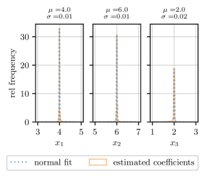
(a) Mono Source

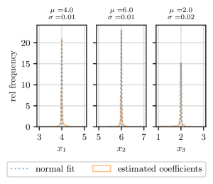
(b) Multiple Sources

Figure 9: Test of coupled ideal Kirchhoff networks, dual Laves-Graph topology, rescaled axis is $x_{i}=\log_{10}\lambda_{i}$, the system was initialized symmetrically with ${x_{1}=4}$ , ${x_{2}=6}$ and ${x_{3}=2}$ for the repulsive case $\varepsilon=-1$. LABEL:sub@fig:murray_par1 : Single source/multi-sink system, parameters histograms and fits $\mathcal{N}(\mu,\sigma)$ presenting the estimated simulation parameters $\lambda_{i}$. LABEL:sub@fig:murray_par5 : Multi-source/multi-sink system, parameters histograms and fits $\mathcal{N}(\mu,\sigma)$ presenting the estimated simulation parameters $\lambda_{i}$.

IV.3 Limited estimation of interaction parameters for sinusoidal networks

Finally we use the extracted graph skeletons of the sinusoids and bile canaliculi in the vicinity of a central vein in the mouse liver to test the generalized Murray’s Law on a real intertwined vessel system. The vascular structure is represented by sets of vertices and edges bearing the positional and radial information of the respective vasculature. We use the same approach as in the prior section to estimate the coupling $\lambda_{1}$, volume penalty $\lambda_{2}$ and fluctuation rate $\lambda_{3}$ for the sinusoidal system. We stress that no information about the actual flow nor the exact point of flow injection or drainage was available. Hence, we first make some simplifying assumptions about the positions of sinks and sources as well as cropping the network skeletons to reduce their complexity: First we identify the vertices in the sinusoidal network which are closest to the central vein and label them as sinks. The geometric center of mass of these vertices is calculated and used as the center of a sphere of radius $R$, representing the range of interest. Any other components, vertices or edges of any network positioned outside this perimeter are discarded (here $R=390\ \mu m$, in order to keep the resulting graphs at a moderate size for computational purposes). Next, all branching points in the sinusoidal network are identified, as are all paths $\boldsymbol{p}=\left(e_{i},...,e_{j}\right)$ consisting of edges $e_{i}$ which start from these points. We proceed for the canaliculi the same way and check for each segment of a path whether there is another segment of another network’s path inside a perimeter $\delta$ (here chosen as $30\ \mu m$). If so, these paths count as affiliated. We merge all edges along a path into a single edge by using the conventional addition theorems for series of conductivities in Kirchhoff networks. Proceeding like this we end up with a reduced sinusoidal network, with $n=318$ vertices and $m=452$ edges. For further details on the reduction procedure see Figure 15 in Appendix D.
We find the parameters $\lambda_{1}$, $\lambda_{2}$, $\lambda_{3}$ numerically by solving equation (34) for randomly sampled tuples of branching points. We do so for a range of exponents $\varepsilon$, under consideration of all sign permutations for $a_{j}$. Hence we probe the system in different coupling regimes and consider all possible flux patterns. The solutions’ histograms as well as the calculated means $\mu\left(x_{i}\right)$ and standard deviations $\sigma\left(x_{i}\right)$ are presented in Figure 10, again using the logarithmic axis rescaling $x_{i}=\log_{10}\lambda_{i}$. We find the histograms to be considerably broadened single peak distributions, indicating relatively stable means for $x_{2}$, $x_{3}$ with varying means of $x_{1}$ for variable exponents $\varepsilon$.
From the previous section III we concluded that attractively coupled networks ($\varepsilon>1$) are able to generate robust, reticulated structures for increased coupling rates of $\lambda_{1}$ and are supported in this by increased fluctuation rates $\lambda_{3}$. The estimates for the attractive coupling case in Figure 10a indicate that increased fluctuation rates are present ($\mu\left(x_{3}\right)>0$) which may account for reticulated structures in flow driven adaption. Further we observe monotonically increasing rates of coupling for increasing $\varepsilon$. Interestingly we find the coupling rates poised just below the actual onset of the topological transition e.g. $\mu\left(x_{1}\right)\pm\sigma\left(x_{1}\right)=2.56\pm 1.04$ for the coupling exponent $\varepsilon=3$.
Further we find the repulsive coupling case to reproduce the same regime of values for $x_{2}$, $x_{3}$, indicating reticulation by flow fluctuation. Yet the coupling parameter $\mu\left(x_{1}\right)$ displays a monotonically decreasing behavior for decreasing values of $\varepsilon$, see Figure 10b. Those low values of $x_{1}$ suggest repulsive interactions to be negligible as the estimates lie far from the regimes with topological implication, e.g. $\mu\left(x_{1}\right)\pm\sigma\left(x_{1}\right)=1.94\pm 1.03$ for the coupling exponent $\varepsilon=-1$.
Unfortunately all estimates $\mu\left(x_{i}\right)$ are accompanied by large standard deviations, which in the logarithmic context, span orders of magnitudes. Further we find no indication for a specific coupling scenario $\varepsilon$, e.g. based on a collapse of the standard deviation for a specific $\varepsilon$, parameter distributions contradicting topological structure, etc. We suspect these issues to originate from several sources: segmentation inaccuracies’ during image analysis, crude approximation of the sink-source landscape of the system, the chosen algorithm of complexity reduction and ambiguity of numeric solutions due to the non-linearity of the problem. Ultimately the very fact that we only make an educated guess about the adaptation mechanisms, might exclude other essential principles of self-organized vessel adaptation in the liver lobule. Nevertheless, considering these findings and the restrictions of our model’s approach we assume the emergence of reticulated sinusoidal structures rather to be the product of flux fluctuations rather than of the newly proposed geometrical interactions. With this technique we have shown that it is possible to extract order of magnitude estimates of otherwise inaccessible parameters of real adapting biological networks, and in doing so to be capable of making qualitative statements about the relative strength or importance of different feedbacks.

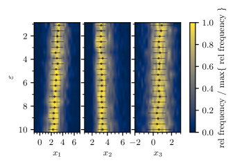
(a) Attractive Coupling

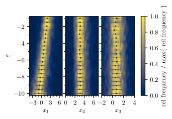
(b) Repulsive Coupling

Figure 10: Estimated parameters for the sinusoidal system near the central vein for $R=397\ \mu m$, $\delta=30\ \mu m$ and rescaled axis $x_{i}=\log_{10}\lambda_{i}$ for different coupling exponents $\varepsilon$.

V Discussion

We have shown that spatial coupling presents another potential mechanism of controlling the topological complexity of optimal transport systems in 3D. We considered the special case of ’single source/multiple sinks’ in combination with simple cubic lattices as plexi as the simplest case possible. In the case of repelling networks we find this interaction to reduce the networks’ relative loop density and provide another method by which a system may be tuned towards its final architecture. It’s also possible to retrieve tree-like states at increased fluctuation levels, which represents a new stabilization mechanism for spanning trees in noisy networks. Nevertheless, the onset of redundancy is primarily driven by the existence of flow fluctuations. On the other hand, we have shown that attracting vessel surfaces allow for the robust emergence of loops on their own. Even the full recovery of the initial plexus is feasible beyond the coupling induced nullity transition, in contrast to what is possible with fluctuations. This presents a new mechanism which allows for the maintenance of dissipation minimized reticulated vessel networks as long as there is an effective scaffold providing a positive growth feedback. No qualitative differences could be found in the phase diagrams in comparison with the dual diamond, or dual Laves graphs. Our model may be interpreted as a toy-model for intertwined flow networks as found in the mammalian liver lobules and other organ structures, such as kidneys, pancreas or bone marrow. The cost function ansatz, though, provides a generally applicable tool in network optimization, and could profitably applied to other boundary conditions or graph geometries which resemble realistic structures.
Our approach further enabled us to derive a more general form Murray’s law, directly involving flow interactions and environmental couplings. We find this technique to predict the model parameters with high fidelity for simulated Kirchhoff networks given their topology and respective edge radii distributions. In the same manner we find order of magnitude estimates for the parameters in experimentally acquired data sets of sinusoids in liver lobule of mice. Hence one could consider this methodology as an effective classification of spatially adapting network structures allowing to probe for relevant parameter regimes of adaptation models.
We aim to expand the purely geometric approach which was studied here, by explicit involvement of hydrodynamic-chemical feedback between a vessel and its local environment. This would be of particular concern in intertwined distribution networks transferring water and metabolites with their respective partner network. Biological systems such as the capillary networks in the liver lobule, present complex dual transport systems where the actual flow rates are not necessarily influenced by their respective partner network’s flow rate Brauer et al. (1954) but rather by the concentration of bile salt components transported Boyer (2013) as well as secretion rates of hepatocytes. Subsequently, future studies should consider concentration/pump-rate dependent flow rate perturbations in the optimization model. One may also consider a direct postulation of cross-network feedback in the adaptation dynamics to account for the actual network structures. Recent studies regarding solute transport and optimization of cross-wall transport Meigel and Alim (2018); Ostrenko et al. (2019) might present a suitable basis for such an approach. Eventually, we strive towards a generalized formulation of environmental factors whose influence can be depicted in the form of local adaptation rules of complex flow networks. Ultimately, complex distribution and flow systems that respect and leverage their spatial embeddings remain a deeply rich topic with myriad opportunities both to make contact with applied and biological settings and to open up new ways to understand the physics of complex systems.

Appendix A Minimization of custom Lyapunov function $\Gamma$

To minimize the cost function $\Gamma$ as given in section II we write it as

$$\Gamma =\Gamma_{12}+\Gamma_{1}+\Gamma_{2}$$ (35)

$$\text{ with }\Gamma_{1} =\frac{\pi}{8\eta_{1}l_{1}}\sum_{e_{1}}\left[\Delta p_{e_{1}}^{2}r_{e_{1}}^{4}+a_{1}r_{e_{1}}^{2}\right]$$ (36)

$$\text{ and }\Gamma_{2} =\frac{\pi}{8\eta_{2}l_{2}}\sum_{e_{2}}\left[\Delta p_{e_{2}}^{2}r_{e_{2}}^{4}+a_{2}r_{e_{2}}^{2}\right]$$ (37)

We may further use the vectorial notation for dissipation-volume terms $\Gamma_{1}$, $\Gamma_{2}$, using (5), to formulate it in terms of the nodal sinks/sources (here just for $\Gamma_{1}$, derivation for $\Gamma_{2}$ is performed analogously),

$$\Gamma_{1} =\Delta\boldsymbol{p}^{T}\cdot\boldsymbol{C}\cdot\Delta\boldsymbol{p}+q\text{ }Tr\left(\boldsymbol{C}^{1/2}\right)$$ (38)

$$=\boldsymbol{s}^{T}\left[\boldsymbol{B}^{T}\boldsymbol{C}\boldsymbol{B}\right]^{\dagger}\boldsymbol{s}+q\text{ }Tr\left(\boldsymbol{C}^{1/2}\right)$$ (39)

with $q=a_{1}\left(\frac{\pi}{8\eta_{1}l_{1}}\right)^{1/2}$ and $c_{e_{1}}=\frac{\pi r_{e_{1}}^{4}}{8\eta_{1}l_{1}}$ as entries of the diagonal $\boldsymbol{C}$. We calculate the (pseudo-)time derivatives of P to be

$$\frac{d\Gamma_{1}}{dt} =\boldsymbol{s}^{T}\partial_{t}\left[\boldsymbol{B}\cdot\boldsymbol{C}\cdot\boldsymbol{B}^{T}\right]^{\dagger}\boldsymbol{s}$$

$$+2\boldsymbol{s}^{T}\left[\boldsymbol{B}\cdot\boldsymbol{C}\cdot\boldsymbol{B}^{T}\right]^{\dagger}\partial_{t}\boldsymbol{s}+q\partial_{t}Tr\left(\boldsymbol{C}^{1/2}\right)$$ (40)

The derivative of the generalized inverse ${\boldsymbol{B}\cdot\boldsymbol{C}\cdot\boldsymbol{B}^{T}=\boldsymbol{A}}$ being Golub and Pereyra (1973),

$$\partial_{t}\boldsymbol{A}^{\dagger} =-\boldsymbol{A}^{\dagger}\left(\boldsymbol{B}\cdot\partial_{t}\boldsymbol{C}\cdot\boldsymbol{B}^{T}\right)\boldsymbol{A}^{\dagger}$$

$$+\left[\boldsymbol{I}-\boldsymbol{A}^{\dagger}\cdot\boldsymbol{A}\right]\left(\boldsymbol{B}\cdot\partial_{t}\boldsymbol{C}\cdot\boldsymbol{B}^{T}\right)\boldsymbol{A}^{T\dagger}\cdot\boldsymbol{A}^{\dagger}$$

$$+\boldsymbol{A}^{\dagger}\cdot\boldsymbol{A}^{T\dagger}\left(\boldsymbol{B}^{T}\cdot\partial_{t}\boldsymbol{C}\cdot\boldsymbol{B}\right)\left[\boldsymbol{I}-\boldsymbol{A}\cdot\boldsymbol{A}^{\dagger}\right]$$ (41)

Fortunately the projector terms vanish as we have,

$$\boldsymbol{s}^{T}\left[\boldsymbol{I}-\boldsymbol{A}^{\dagger}\cdot\boldsymbol{A}\right]=0\text{ and }\left[\boldsymbol{I}-\boldsymbol{A}\cdot\boldsymbol{A}^{\dagger}\right]\boldsymbol{s}=0$$ (42)

Together with the identity $\boldsymbol{A}^{\dagger}=\left(\boldsymbol{A}^{T}\right)^{\dagger}$ the total time-derivative of $\Gamma_{1}$ becomes,

$$\frac{d\Gamma_{1}}{dt} =-\boldsymbol{s}^{T}\boldsymbol{A}^{T\dagger}\left(\boldsymbol{B}\cdot\partial_{t}\boldsymbol{C}\cdot\boldsymbol{B}^{T}\right)\boldsymbol{A}^{\dagger}\boldsymbol{s}$$

$$+2\boldsymbol{s}^{T}\boldsymbol{A}^{\dagger}\partial_{t}\boldsymbol{s}+q\partial_{t}Tr\left(\boldsymbol{C}^{1/2}\right)$$ (43)

With partial derivatives simplifying this formula as:

$$\partial_{t}Tr\left(\boldsymbol{C}^{1/2}\right) =\frac{1}{2}Tr\left(\boldsymbol{C}^{-1/2}\cdot\partial_{t}\boldsymbol{C}\right)$$ (44)

$$\partial_{t}\boldsymbol{s} =0$$ (45)

As we also have $\Delta\boldsymbol{p}=\boldsymbol{B}^{T}\cdot\boldsymbol{A}^{\dagger}\boldsymbol{s}$, we may write the total time-derivative as

$$\frac{d\Gamma_{1}}{dt}=-\Delta\boldsymbol{p}^{T}\cdot\partial_{t}\boldsymbol{C}\cdot\Delta\boldsymbol{p}+\frac{q}{2}Tr\left(\boldsymbol{C}^{-1/2}\partial_{t}\boldsymbol{C}\right)$$ (46)

With diagonals $\partial_{t}c_{e_{1}}=\frac{\pi r^{3}_{e_{1}}}{2\eta_{1}l_{1}}\partial_{t}r_{e_{1}}$ and re-substituting $q$ this becomes

$$\frac{d\Gamma_{1}}{dt}=\frac{\pi}{2\eta_{1}l_{1}}\sum_{e_{1}}r_{e_{1}}\left[\frac{a_{1}}{2}-\Delta p_{e_{1}}^{2}r_{e_{1}}^{2}\right]\partial_{t}r_{e_{1}}$$ (47)

The coupling component’s derivative $\Gamma_{12}$ may be calculated with partial derivatives,

$$\frac{d\Gamma_{12}}{dt}=-\frac{b\varepsilon}{2}\left[\sum_{e_{1}e_{2}}F_{e_{1}e_{2}}\Delta r_{e_{1}e_{2}}^{\varepsilon-1}\partial_{t}r_{e_{1}}+\sum_{e_{1}e_{2}}F_{e_{1}e_{2}}\Delta r_{e_{1}e_{2}}^{\varepsilon-1}\partial_{t}r_{e_{2}}\right]$$ (48)

so combining (47) and (48) we get for the total derivative of $\Gamma$,

$$\frac{d\Gamma}{dt} =\frac{\pi}{2\eta_{1}l_{1}}\sum_{e}r_{e_{1}}\left[\frac{a_{1}}{2}-\Delta p_{e_{1}}^{2}r_{e_{1}}^{2}\right]r_{e_{1}}\partial_{t}r_{e_{1}}$$

$$+\frac{\pi}{2\eta_{2}l_{2}}\sum_{e_{2}}\left[\frac{a_{2}}{2}-\Delta p_{e_{2}}^{2}r_{e_{2}}^{2}\right]r_{e_{2}}\partial_{t}r_{e_{2}}$$

$$-\frac{b\varepsilon}{2}\left[\sum_{e_{1}}F_{e_{1}e_{2}}\Delta r_{e_{1}e_{2}}^{\varepsilon-1}\partial_{t}r_{e_{1}}+\sum_{e_{2}}F_{e_{1}e_{2}}\Delta r_{e_{1}e_{2}}^{\varepsilon-1}\partial_{t}r_{e_{2}}\right]$$ (49)

To find a local minimum of $\Gamma$ when progressing through (pseudo-)time $t$ we have to ensure that $d\Gamma\leq 0$. So we may minimize $\Gamma$, with auxiliary functions $\chi_{i}\geq 0$ by choosing

$$\partial_{t}r_{e_{1}}/\chi_{1} =\left[\Delta p^{2}_{e_{1}}r_{e_{1}}^{2}-\alpha_{1}\right]r_{e_{1}}+\beta_{1}\operatorname{sgn}(\varepsilon)\sum_{e_{2}}F_{e_{1}e_{2}}\Delta r_{e_{1}e_{2}}^{\varepsilon-1}$$ (50)

$$\partial_{t}r_{e_{2}}/\chi_{2} =\left[\Delta p^{2}_{e_{2}}r_{e_{2}}^{2}-\alpha_{2}\right]r_{e_{2}}+\beta_{2}\operatorname{sgn}(\varepsilon)\sum_{e_{1}}F_{e_{1}e_{2}}\Delta r_{e_{1}e_{2}}^{\varepsilon-1}$$ (51)

where we set ${\alpha_{i}=\frac{a_{i}}{2}}$, ${\beta_{i}=\frac{b\eta_{i}l_{i}|\varepsilon|}{\pi}}$ for compact notation.

Appendix B Uncorrelated and coupled flow fluctuations

In this section we give a detailed derivation of the analytic form of the mean squared pressure in case of uncorrelated, identically distributed sink fluctuations as introduced in Corson (2010) and discussed in section II.
From the current law (1) in combination with Ohm’s law (2) one knows that the sum over all in and outflows of the system vanishes Duffin (1959), i.e. $\sum_{v}s_{v}=0$. When considering the sink conditions as well as the source constraint defined in the theory section, we may write the moments as (putting the distinguished source at $v=0$),

$$\left<s_{v}\right> =\mu$$ (52)

$$\left<s_{0}\right> =-\left<\sum_{v>0}s_{v}\right>=\left(1-n\right)\mu$$ (53)

$$\left<s_{v}s_{w}\right> =\delta_{vw}\sigma^{2}+\mu^{2}\text{ if }v,w>0$$ (54)

$$\left<s_{0}^{2}\right> =\left<\sum_{v,w>0}s_{v}s_{w}\right>=\left(n-1\right)\sigma^{2}+\left(n-1\right)^{2}\mu^{2}$$ (55)

$$\left<s_{0}s_{w}\right> =-\left<\sum_{v>0}s_{v}s_{w}\right>=-\left(n-1\right)\mu^{2}-\sigma^{2}$$ (56)

Hence we may calculate the squared-mean pressure by using the auxiliary conductivity tensor ${\boldsymbol{A}^{e}_{vw}=\boldsymbol{C}^{-1}_{ee}\left[\boldsymbol{B}\cdot\boldsymbol{C}^{1/2}\right]_{ev}^{\dagger}\left[\boldsymbol{B}\cdot\boldsymbol{C}^{1/2}\right]_{ew}^{\dagger}}$ as,

$$\left<\Delta p_{e}^{2}\right>= \sum_{vw}\boldsymbol{A}^{e}_{vw}\left<s_{v}s_{w}\right>$$ (57)

$$= \boldsymbol{A}^{e}_{00}\left<s_{0}^{2}\right>+2\sum_{v>0}\boldsymbol{A}^{e}_{v0}\left<s_{0}s_{v}\right>+\sum_{v,w>0}\boldsymbol{A}^{e}_{vw}\left<s_{v}s_{w}\right>$$ (58)

$$= \boldsymbol{A}^{e}_{00}\left(n-1\right)\left[\left(n-1\right)\mu^{2}+\sigma^{2}\right]$$

$$-2\sum_{v>0}\boldsymbol{A}^{e}_{v0}\left[\left(n-1\right)\mu^{2}+\sigma^{2}\right]$$

$$+\sum_{v,w>0}\boldsymbol{A}^{e}_{vw}\left[\delta_{vw}\sigma^{2}+\mu^{2}\right]$$ (59)

$$= \sum_{v,w}\boldsymbol{A}^{e}_{vw}\left(n-1\right)\left[\left(n-1\right)\mu^{2}+\sigma^{2}\right]\delta_{0v}\delta_{0w}$$

$$-\sum_{v,w}\boldsymbol{A}^{e}_{vw}\left[\left(n-1\right)\mu^{2}+\sigma^{2}\right]\left[\left(1-\delta_{0w}\right)\delta_{0v}\right]$$

$$-\sum_{v,w}\boldsymbol{A}^{e}_{vw}\left[\left(n-1\right)\mu^{2}+\sigma^{2}\right]\left[\left(1-\delta_{0v}\right)\delta_{0w}\right]$$

$$+\sum_{v,w}\boldsymbol{A}^{e}_{vw}\left[\delta_{vw}\sigma^{2}+\mu^{2}\right]\left(1-\delta_{0v}\right)\left(1-\delta_{0w}\right)$$ (60)

Ordering the terms for $\mu$ and $\sigma$ respectively we can acquire the coefficient matrices $\boldsymbol{U}$ and $\boldsymbol{V}$,

$$\left<\Delta p_{e}^{2}\right>=\sum_{v,w}\boldsymbol{A}^{e}_{vw}\mu^{2}\left[\left(1-\delta_{0v}\right)\left(1-\delta_{0w}\right)+\delta_{0v}\delta_{0w}\left(n-1\right)^{2}\right.$$

$$\left.-\left(n-1\right)\left(\delta_{0v}\left(1-\delta_{0w}\right)+\delta_{0w}\left(1-\delta_{0v}\right)\right)\vphantom{\left(n-1\right)^{2}}\right]$$

$$+\sum_{v,w}\boldsymbol{A}^{e}_{vw}\sigma^{2}\left[\left(1-\delta_{0w}\right)\left(1-\delta_{0v}\right)\delta_{vw}-\delta_{0v}\left(1-\delta_{0w}\right)\right.$$

$$\left.-\delta_{0w}\left(1-\delta_{0v}\right)+\left(n-1\right)\delta_{0v}\delta_{0w}\right]$$ (61)

$$=\sum_{v,w}\boldsymbol{A}^{e}_{vw}\mu^{2}\left[1+\delta_{0v}\delta_{0w}n^{2}-n\left(\delta_{0v}+\delta_{0w}\right)\right]$$

$$+\sum_{v,w}\boldsymbol{A}^{e}_{vw}\sigma^{2}\left[\delta_{vw}+\left(n+1+\delta_{vw}\right)\delta_{0v}\delta_{0w}\right.$$

$$\left.-\left(1+\delta_{vw}\right)\left(\delta_{0v}+\delta_{0w}\right)\right]$$ (62)

We further suggest to expand this ansatz by introducing additional sources which act as clones of the very first one, i.e. we will have $s_{p}=s_{q}$ using the indices $p,q$ for sources and $m,n$ for sinks. Then conditions (53), (55),(56) will become for $a$ sources and $b$ sinks (with $a+b=n$),

$$\left<\sum_{p}s_{p}\right> =-\left<\sum_{u}s_{u}\right>=-b\mu\rightarrow\left<s_{p}\right>=-\frac{b}{a}\mu$$ (63)

$$\left<s_{p}s_{q}\right> =\frac{1}{a^{2}}\left<\sum_{u,v}s_{u}s_{v}\right>=\frac{1}{a^{2}}\left(b\sigma^{2}+b^{2}\mu^{2}\right)$$ (64)

$$\left<s_{p}s_{u}\right> =-\frac{1}{a}\left<\sum_{v}s_{v}s_{u}\right>=-\frac{1}{a}\left(b\mu^{2}-\sigma^{2}\right)$$ (65)

And hence we may calculate the mean squared pressure and its coefficient matrices respectively as,

$$\left<\Delta p_{e}^{2}\right>=\sum_{v,w}\boldsymbol{A}^{e}_{vw}\mu^{2}\left[\frac{b^{2}}{a^{2}}\sum_{p,q}\delta_{pv}\delta_{qw}\right.$$

$$\left.-\frac{b}{a}\sum_{p,m}\left(\delta_{pv}\delta_{mw}+\delta_{mv}\delta_{pw}\right)+\sum_{m,n}\delta_{mv}\delta_{nw}\right]$$

$$+\sum_{v,w}\boldsymbol{A}^{e}_{vw}\sigma^{2}\left[\frac{b}{a^{2}}\sum_{p,q}\delta_{pv}\delta_{qw}\right.$$

$$\left.-\frac{1}{a}\sum_{p,m}\left(\delta_{pv}\delta_{mw}+\delta_{mv}\delta_{pw}\right)+\sum_{m,n}\delta_{mv}\delta_{nw}\delta_{mn}\right]$$ (66)

Appendix C Simulating coupled, adapting networks

In this section we show additional material of the simulations’ results as performed in section III for both of the networks in comparison. In Figure 11 and 12 we display the nullity transition curves for the cases of repulsive and attractive coupling. It may be noted here once again that all simulation parameters $\lambda_{i}$ were initialized identically for the two networks, meaning any deviations in $\varrho$ have to be caused by topological differences. This phenomenon is particularly apparent in the case of attractive coupling in cubic lattices where the nullity transition in the respective networks becomes smeared out differently for the two structures. Repeating the simulations for coupled networks consisting of complimentary Laves graphs or diamond lattices, we find this effect negligible.

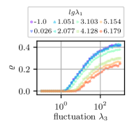
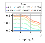
(a) Network # 1

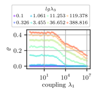
(b) Network # 2

Figure 11: Nullity $\varrho$ transitions for repulsively coupled networks ($\varepsilon=-1)$: Symmetric fluctuation $\lambda_{3}$ induced nullity onset and coupling $\lambda_{1}$ induced nullity breakdown for the two networks LABEL:sub@fig:bilayer_nullity_supplement_a and LABEL:sub@fig:bilayer_nullity_supplement_b

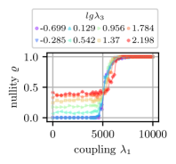
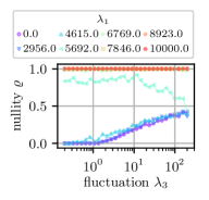
(a) Network # 1

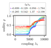
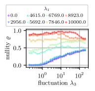
(b) Network # 2

Figure 12: Nullity $\varrho$ transitions for attractively coupled networks ($\varepsilon=3)$: Slightly asymmetric coupling $\lambda_{1}$ induced nullity onset and fluctuation $\lambda_{3}$ induced nullity transition for the two networks LABEL:sub@fig:bilayer_nullity_supplement_c and LABEL:sub@fig:bilayer_nullity_supplement_d

In the case of repulsive coupling (Fig. 13a, 13b), both networks display a shift of the onset of fluctuation induced loops as well as a shift of the estimated saturation point. It may be noted though that a change of several orders of magnitude in the coupling $\lambda_{1}$ is necessary in order to shift the fluctuation onset at all. It is nevertheless crucial to note that the overall nullity is reduced even in the saturated case which itself tends to be achieved only for significantly higher fluctuations $\lambda_{3}$. A similar trend of shifting may be observed in the case of attractive coupling (Fig. 13c, 13d). The onset of full plexus recovery as well as the saturation onset develop on similar scales. Note that the trajectories for network # 2 suggest the possibility of re-entrant behaviour between coupling and fluctuation dominated nullity regimes.

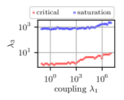
(a) Network # 1

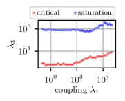
(b) Network # 2

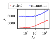
(c) Network # 1

(d) Network # 2

Figure 13: LABEL:sub@fig:bilayer_onset_supplement_1a + LABEL:sub@fig:bilayer_onset_supplement_1b Shift of onset and saturation points of the fluctuation $\lambda_{3}$ induced nullity transitions shift for repulsive coupling, here displayed for negative coupling exponent $\varepsilon=-1$. LABEL:sub@fig:bilayer_onset_supplement_2a + LABEL:sub@fig:bilayer_onset_supplement_2b Shift of onset and saturation points of the attractive coupling $\lambda_{1}$ induced nullity transitions shift for varying fluctuation $\lambda_{3}$, here displayed for positive coupling exponent $\varepsilon=3$

Appendix D Scaling laws in coupled, noisy networks

This section is focused on the geometric law discussed in section IV. One can show that introducing fluctuations and coupling alter the classical form of Murray’s Law $r_{0}^{3}=r_{1}^{3}+r_{2}^{3}$ in the following way: Given the Kirchhoff current law and rewriting it via Ohm’s law, we get for all sink-vertices $i$,

$$\sum_{e\in\operatorname{inc}(v)}f_{e}=s_{v}\Leftrightarrow \sum_{e\in\operatorname{inc}(v)}r_{e}^{*4}\Delta p_{e}^{*}=s_{v}^{*}$$ (67)

Taking the average over all pressure configurations between two adaptation events we get

$$\sum_{e\in\operatorname{inc}(v)}r_{e}^{*4}\left<\Delta p_{e}^{*}\right>=\left<s_{v}^{*}\right>\Leftrightarrow \sum_{e\in\operatorname{inc}(v)}\Theta_{ve}r_{e}^{*4}|\left<\Delta p_{e}^{*}\right>|=\left<s_{v}^{*}\right>$$ (68)

with an effective incidence factor $\Theta_{ve}=\begin{cases}\pm 1\\ 0\end{cases}$ distinguishing between in- and outgoing flows on the relevant edges, see Figure 14. In order to acquire the cubic form we substitute $r_{e}^{*}$ with the result of the stationary state’s equations,

$$\partial_{t^{*}}r_{e}^{*} =0$$ (69)

$$\Rightarrow 0 =\left(r_{e}^{*2}\left<\Delta p_{e}^{*2}\right>-\lambda_{2}\right)r_{e}^{*}+\lambda_{1}\operatorname{sgn}(\varepsilon)\sum_{e^{\prime}}F_{ee^{\prime}}\Delta r_{ee^{\prime}}^{*,-\varepsilon}$$ (70)

$$\Leftrightarrow r_{e}^{*} =\frac{\sqrt{\lambda_{2}-\lambda_{1}r_{e}^{*-1}\operatorname{sgn}(\varepsilon)\sum_{e^{\prime}}F_{ee^{\prime}}\Delta r_{ee^{\prime}}^{*,\varepsilon-1}}}{\sqrt{\left<\Delta p_{e}^{*2}\right>}}$$ (71)

Figure 14: Scheme of identifying different flow combinations at a sink determining the respective sign of $\Theta_{ve}$, here shown for Y-branching point. Let’s identify the sink as $i=0$ and and the respective flow carrying edges as $e\in\{1,2,3\}$ and define an incidence triplet $\boldsymbol{\Theta}=\left(\Theta_{01},\Theta_{02},\Theta_{03}\right)$. Reading from left to right we have in the top diagram:
$\boldsymbol{\Theta}=\left(1,-1,-1\right)$, $\boldsymbol{\Theta}=\left(1,1,-1\right)$
Middle diagram:
$\boldsymbol{\Theta}=\left(1,-1,1\right)$, $\boldsymbol{\Theta}=\left(1,1,1\right)$, $\boldsymbol{\Theta}=\left(-1,1,-1\right)$
Bottom diagram:
$\boldsymbol{\Theta}=\left(-1,-1,1\right)$, $\boldsymbol{\Theta}=\left(-1,1,1\right)$

Plugging (71) into (68) and rewriting ${|\left<\Delta p_{e}^{*}\right>|=\sqrt{\left<\Delta p_{e}^{*}\right>^{2}}}$, ${g^{*}_{e}\left(\varepsilon\right)=\operatorname{sgn}(\varepsilon)\sum_{e^{\prime}}F_{ee^{\prime}}\Delta r_{ee^{\prime}}^{*,\varepsilon-1}}$ we get,

$$\sum_{e\in inc(v)}\Theta_{ve}\sqrt{\left(\lambda_{2}-\lambda_{1}r_{e}^{*-1}g^{*}_{e}\left(\varepsilon\right)\right)\frac{\left<\Delta p_{e}^{*}\right>^{2}}{\left<\Delta p_{e}^{*2}\right>}}r_{e}^{*3}=\left<s_{v}^{*}\right>$$ (72)

We know from section B that $\left<\Delta p_{e}^{2}\right>=\sum_{vw}\boldsymbol{A}^{e}_{vw}\left<s_{v}s_{w}\right>$ and may also deduce ${\left<\Delta p_{e}\right>^{2}=\sum_{vw}\boldsymbol{A}^{e}_{vw}\left<s_{v}\right>\left<s_{w}\right>}$. This enables us to calculate the ratio via the covariance,

$$\frac{\left<\Delta p_{e}^{2}\right>}{\left<\Delta p_{e}\right>^{2}} =\frac{\sum_{vw}\boldsymbol{A}^{e}_{vw}\left<s_{v}s_{w}\right>}{\sum_{vw}\boldsymbol{A}^{e}_{vw}\left<s_{v}\right>\left<s_{w}\right>}$$ (73)

$$=\frac{\sum_{vw}\boldsymbol{A}^{e}_{vw}\left[\left<s_{v}\right>\left<s_{w}\right>+\left<\left(s_{v}-\left<s_{v}\right>\right)\left(s_{w}-\left<s_{w}\right>\right)\right>\right]}{\sum_{vw}\boldsymbol{A}^{e}_{vw}\left<s_{v}\right>\left<s_{w}\right>}$$ (74)

$$=1+\frac{\sum_{vw}\boldsymbol{A}^{e}_{vw}\left<\left(s_{v}-\left<s_{v}\right>\right)\left(s_{w}-\left<s_{w}\right>\right)\right>}{\sum_{vw}\boldsymbol{A}^{e}_{vw}\left<s_{v}\right>\left<s_{w}\right>}$$ (75)

Substituting this into (72) and having $\frac{\left<\Delta p_{e}^{2}\right>}{\left<\Delta p_{e}\right>^{2}}=\frac{\left<\Delta p_{e}^{*2}\right>}{\left<\Delta p_{e}^{*}\right>^{2}}$, $H_{e}=\frac{\sum_{vw}\boldsymbol{A}^{e}_{vw}\left<\left(s_{v}-\left<s_{v}\right>\right)\left(s_{w}-\left<s_{w}\right>\right)\right>}{\sum_{vw}\boldsymbol{A}^{e}_{vw}\left<s_{v}\right>\left<s_{w}\right>}$ we get,

$$\sum_{e\in\operatorname{inc}(v)}a_{e}r_{e}^{*3}=\left<s_{v}^{*}\right>$$ (76)

$$\text{ setting }a_{e}=\Theta_{ve}\sqrt{\frac{\lambda_{2}-\lambda_{1}r_{e}^{*-1}g^{*}_{e}\left(\varepsilon\right)}{1+H_{e}}}$$ (77)

One may simplify this complex by considering the following: Assume that we have all randomly fluctuating sinks distributed uncorrelated yet identically as in section B, (62), then we may set $\left<s_{v}^{*}\right>=1$ and reevaluate $H_{e}$. This leads to the equation presented in section IV,

$$\sum_{\in\operatorname{inc}(v)}a_{e}r_{e}^{*3} =1$$ (78)

$$\text{ with }a_{e} =\Theta_{ve}\sqrt{\frac{\lambda_{2}-\lambda_{1}r_{e}^{*-1}g^{*}_{e}\left(\varepsilon\right)}{1+\lambda_{3}\frac{\delta\phi_{e}}{\phi_{e}}}}$$ (79)

For experimental validation of (78) it will be necessary to know the networks vessel radii as well as the sink/source pattern (although it may be sufficient to know where the system’s source is and to consider every other node as sink). Considering Y-branchings of low sink/source value (points of negligible secretion/leakage) such that $|a_{e}r_{e}^{*,3}|\gg 1$, further setting the index for the largest vessel to zero ( and accordingly increasing for the other vessel pieces at the branching) may write,

$$a_{0}r^{*3}_{0}=a_{1}r^{*3}_{1}+a_{2}r^{*3}_{2}$$ (80)

In Figure 15 we show the applied reduction procedure as used in the section IV.3.

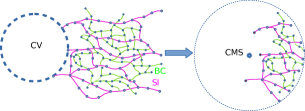
(a)

(b)

Figure 15: Setting the range of interest and coarse-graining the sinusoidal (SI) and bile canaliculi system (BC): LABEL:sub@fig:sketch_roi Left: Vertices closest to the central vein (CV) are identified as sinks. Right: Determine geometric center of mass of all sinks (CMS) and discard all components, vertices, edges outside a set perimeter. LABEL:sub@fig:sketch_coarse Left: Deducting the distance of one path of a network to another path of the partner network by calculating the pair-wise distances of all path-segments and finding its minimum. Right: Coarse-graining paths into one effective edge, with new edge weight according to addition theorem $c^{*}_{eff}=\sum_{e}\frac{1}{c^{*}_{e}}$.

First, the vertices in the sinusoidal network (SI) which are closest to the central vein (CV) are identified. Using these a geometric center of mass(CMS) is calculated and used as the center of a sphere of radius $R$, representing the range of interest (ROI). Any other components, vertices or edges of any network positioned ROI, see Figure 15a. Next, all branching points in the sinusoidal network are identified and all paths $\boldsymbol{p}=\left(e_{i},...,e_{j}\right)$ consisting of edges $e_{i}$ which start from these points. We proceed for the canaliculi the same way and then check for each segment of a path $\boldsymbol{p}$ whether there is another segment of another network’s path $\boldsymbol{p}^{\prime}$ inside a perimeter $\delta$ . If so, these paths count as affiliated. Then we merge all edges along a path towards a single edge by using the conventional addition theorems for series of conductivities, as $c_{eff}=\sum_{e}\frac{1}{c_{e}}$, see Figure 15b. When confronted with datasets of real spatial transport network such as blood capillaries and secretion channels in IV.3 it becomes important to note that the chosen ROI, namely the radius $R$ and the affiliation perimeter $\delta$ will affect the estimation of the parameters $x_{i}=\log\left(\lambda_{i}\right)$.

Figure 16: Histogram displaying the number of affiliated neighbors (edges) found for a given radius around a vessel (threshold, all values the inset in $\mu m$). Total number of pairings found overall for given threshold in the inset for set range of interest $R=397\ \mu m$.

For example see Figure 16, increasing the affiliation parameter $\delta$ will naturally increase the number of edges affiliated with each other, possibly linking vessel structures of several consecutive neighborhoods.
Further we attempt to screen through the range of potential coupling exponents $\varepsilon$ in order to find the $\lambda_{i}$ distributions as displayed in Figure 10, section IV.3. In Figure 17 we display the explicit distributions for selected $\varepsilon$ depicting the different coupling regimes. We smooth the datasets with a Savitzky-Golay filter (red fit line in 17) and identify the local maxima which display a prominence of at least $10\%$ of the maximal function value. We subsequently use Gaussian fits at the identified peak’s positions to acquire the mean values and standard deviations as depicted in 17b,17d.

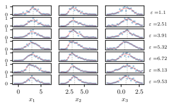
(a)

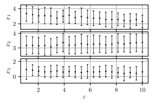
(b)

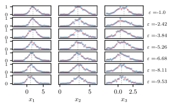
(c)

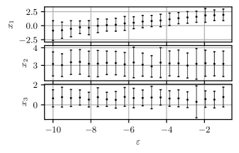
(d)

Figure 17: Estimated parameter distributions with rescaled axis $x_{i}=\log_{10}\lambda_{i}$ (in blue) for selected $\varepsilon$ in the sinusoidal system for $R=397\ \mu m$, $\delta=30\ \mu m$. Applied a Savitzky-Golay regression (in red) to enable an effective peak identification. Subsequently, Gaussian fits are used to calculate the means and standard deviations of the smoothed distributions. LABEL:sub@fig:hist_attractive + LABEL:sub@fig:epsilon_attractive : Attractive Coupling LABEL:sub@fig:hist_repulsive + LABEL:sub@fig:epsilon_repulsive : Repulsive Coupling