Group velocity distribution and short-pulse dispersion in a disordered transverse Anderson localization optical waveguide

Abstract

We investigate the group velocity distribution of waveguide modes in the presence of disorder. The results are based on extensive numerical simulations of disordered optical waveguides using statistical methods. We observe that the narrowest distribution of group velocities is obtained in the presence of a small amount of disorder; therefore, the modal dispersion of an optical pulse is minimized when there is only a slight disorder in the waveguide. The absence of disorder or the presence of a large amount of disorder can result in a large modal dispersion due to the broadening of the distribution of the group velocities. We devise a metric that can be applied to the mode group index probability-density-function and predict the optimal level of disorder that results in the lowest amount of modal dispersion for short pulse propagation. Our results are important for studying the propagation of optical pulses in the linear regime, e.g., for optical communications; and the nonlinear regime for high-power short-pulse propagation.

I Introduction

Transverse Anderson localization (TAL) of light was first proposed by Abdullaev, et al. transverse-Abdullaev and De Raedt, et al. transverse-DeRaedt in a dielectric medium with a transversely random and longitudinally uniform refractive index profile. They showed that an optical beam can propagate freely in the longitudinal direction while being trapped (Anderson-localized Anderson1 ; Anderson1980 ; Abrahams-50-book ; Lagendijk-Physics-Today-2009 ; Abrahams-Scaling-Theory ; Stone ; sheng2006introduction ) in the disordered transverse direction(s). TAL of light has since been observed in various optical systems with one or two transversely disordered dimensions Schwartz2007 ; Lahini-1D-AL-2008 ; Martin-1D-AL-2011 ; Mafi-Salman-OL-2012 ; Mafi-Salman-OPEX-2012 ; Mafi-Salman-OMEX-2012 ; SegevNaturePhotonicsReview ; Mafi-AOP-2015 ; fratini2015anderson ; yao2017beam ; yilmaz2019transverse ; PhysRevA.99.063807 . In particular, Karbasi, et al. reported the first observation of TAL in disordered optical fibers Mafi-Salman-OL-2012 ; Mafi-Salman-OPEX-2012 ; Mafi-Salman-OMEX-2012 . The disordered optical fibers have since been used for high-quality image transport Mafi-Salman-Nature-2014 ; Tuan:18 ; tong2018characterization ; zhao2018image ; zhao2018deep , beam multiplexing Mafi-Salman-Multiple-Beam-2013 , wave-front shaping and sharp focusing Mafi-Marco-singlemode-2017 ; Mafi-Marco-Nature-light-focusing-2014 ; Mafi-Behnam-Optica-2018 , nonlocal nonlinearity Mafi-Marco-APL-self-focusing-2014 ; Mafi-Marco-PRL-Migrating-NL-2014 , single-photon data packing Mafi-Marco-information-2016 , optical diagnostics liang2018surface , and random lasers Mafi-Behnam-Random-Laser-2017 ; joshi2019effect .

TAL optical fiber (TALOF) is essentially a highly multimode optical fiber (MMF) with a transversely random refractive index profile. What sets a TALOF apart from a conventional MMF is that its guided modes are spatially localized due to the transverse disorder, while the guided modes in a conventional MMF typically cover all or a large portion of the guiding region okamoto2005fundamentals ; gloge1973multimode ; Feit:78 . The modal characteristics of MMFs are generally responsible for their performance for the desired functionality jolivet2009beam ; vcivzmar2012exploiting ; papadopoulos2013high ; amitonova2016high ; zhu2010coherent ; e.g., the mean localization radius of the modes in an imaging TALOF determines the average point spread function (PSF) across the tip of the fiber, where a stronger localization leads to a narrower PSF and a higher resolution image transport Mafi-Salman-Nature-2014 . Similarly, the standard deviation in the localization radius of the modes determines the uniformity of the image transport across the fiber. Because the refractive index profile of a TALOF is random and the guided modes are numerous, the modal characteristics of a TALOF must be studied statistically Mafi-AOP-2015 ; Mafi-Salman-Modal-JOSAB-2013 . This stochastic nature of TALOFs and the diversity of the physical attributes of the localized modes is the key differentiating factor between the linear/nonlinear dynamics observed in TALOFs versus conventional MMFs.

The modal area statistics of disordered quasi-one-dimensional (quasi-1D) and quasi-two-dimensional optical waveguides were studied recently by Abaie, et al. Mafi-Behnam-Scaling-PRB-2016 ; Mafi-Abaie-OL-2018 using the mode-area probability-density-function (PDF). The mode-area PDF characterizes the relative distribution of the mode-areas of the guided modes in a disordered waveguide. In particular, Abaie, et al. showed that the mode-area PDF converges to a terminal configuration as the transverse dimensions of the waveguide are increased. Therefore, it may not be necessary to study a real-sized disordered structure to obtain its full statistical localization properties and the PDF can be obtained for a considerably smaller structure. This observation is not only important from a fundamental standpoint, it has practical implications because it can reduce the often demanding computational cost that is required to study the statistical properties of Anderson localization in disordered waveguides. We emphasize that the mode-area PDF encompasses all the relevant statistical information on spatial localization of the guided modes and is a powerful tool for studying the TAL. In this paper, we employ a similar statistical analysis based on the probability-density-function to study the dispersive properties of TAL in disordered waveguides.

In the modal language, the dispersive properties of a waveguide are determined by the frequency ($\omega$) dependence of the propagation constant, $\beta(\omega)$, of the guided modes agrawal2013nonlinear ; agrawal2012fiber . Determining the optical dispersive properties of TALOFs is critical to the understanding of their linear and nonlinear characteristics, or in the continuous wave (CW) or pulsed laser operation, a few examples of which are as follows. For each mode labeled with an index $i$, the full form of $\beta_{i}(\omega)$ over a broad frequency range is needed to determine the phase-matching wavelengths for the intermodal (nonlinear) four-wave mixing (FWM) process stolen1974phase ; lin1981large ; hill1981efficient ; Pourbeyram:15 ; Nazemosadat:13 . In some cases, the Taylor expansion of $\beta(\omega)$ around a central frequency of $\omega_{0}$ and the corresponding local frequency derivatives, $\beta^{(n)}_{i}=\partial^{n}_{\omega}\beta_{i}|_{\omega_{0}}$, are sufficient to characterize the dispersive properties of an optical fiber agrawal2013nonlinear ; agrawal2012fiber . For example, consider $\beta^{(1)}_{i}(\omega)$, which determines the group velocity associated with the mode labeled with the index $i$: in the linear regime, the difference between group velocities of different modes in a multimode fiber is responsible for the intermodal dispersion, which is generally the main limiting factor for the achievable transmission bandwidth (data-rate) in a multimode optical fiber communications system agrawal2012fiber ; gloge1973impulse ; fan2005principal . When an optical pulse is sent through a MMF, the intermodal dispersion (different values of $\beta^{(1)}_{i}$ for different modes) causes the pulse to break into multiple sub-pulses, each propagating with a different group velocity. Therefore, the distribution of group velocities determines the achievable data-rate. For example, a nanosecond-long optical pulse is hardly affected by the propagation through a 1 km-long high-quality graded index fiber Olshansky:76 ; koike1995high ; however, the same pulse is highly distorted by the modal dispersion in a comparable step-index optical fiber. $\beta^{(1)}_{i}(\omega)$ also determines the pulsed nonlinear dynamics, including that of soliton propagation in MMF WiseA5 ; WiseA13 ; Raghavan . For CW laser applications, the cavity response, including the free spectral range (FSR), is determined by the values of $\beta_{i}(\omega)$ for the relevant modes, which are excited in the lasing process; their distribution can dictate the spectrum of the laser via the optical Vernier effect Vasdekis:07 ; EsmaeilSelectivity . The pulsed dynamics of such lasers, including the Q-switching and mode-locking, are similarly controlled by the values of $\beta^{(1)}_{i}(\omega)$ for the relevant modes Mafi-Behnam-Random-Laser-2017 .

I.1 Studying a quasi-1D disordered slab waveguide

In this manuscript, we focus on the statistics of the groups velocity (GV) of the guided modes and determine the GV-PDF of disordered waveguides. Understanding the GV distribution underlies a large number of dispersive phenomena in guided wave systems ho2011statistics . Solving for all the guided modes for a given TALOF and obtaining proper statistical averages over many fiber samples is a formidable task even for large computer clusters. For example, the V-number of the disordered polymer TALOF in Ref. Mafi-Salman-OL-2012 with an air cladding is approximately 2,200 at 405 nm wavelength resulting in more than 2.3 million guided modes. Recall that the V-number is given by

$$V=\dfrac{\pi t}{\lambda}\sqrt{n^{2}_{\rm co}-n^{2}_{\rm cl}},$$ (1)

where $\lambda$ is the optical wavelength, $t$ is the core diameter of the fiber (or the core width for the case of a quasi-1D slab waveguide), and $n_{\rm co}$ ($n_{\rm cl}$) is the effective refractive index of the core (cladding). The total number of the bound guided modes in a step-index optical fiber is $\approx V^{2}/2$. As such, in order to lay the groundwork for understanding the statistical behavior of GV distribution in TALOFs, we have decided to present a comprehensive characterization of a quasi-1D Anderson localized optical waveguide in this manuscript. This exercise is quite illuminating as it sheds light on the general statistical behavior of GV distribution and shows the extent of information that can be extracted from such distributions. The detailed analysis of the TALOF structure will be presented in a future publication.

I.2 Wave equation for the guided modes

Here, we have chosen to calculate the transverse electric (TE) modes of the disordered waveguide using the finite element method (FEM) presented in Refs. Mafi-Behnam-Boundary-OC-2016 ; El-Dardiry-microwave-2012 ; Kartashov-NL-2012 ; Lenahan . Similar observations can be drawn for transverse magnetic (TM) guided modes, but we limit our analysis to TE in this paper for simplicity. The appropriate partial differential equation that will be solved in this manuscript is the Helmholtz equation for electromagnetic wave propagation in a z-invariant dielectric waveguide

$$\nabla^{2}_{\rm T}A({\bf x}_{\rm T})+n^{2}({\bf x}_{\rm T})k_{0}^{2}A({\bf x}_{\rm T})=\beta^{2}A({\bf x}_{\rm T}),$$ (2)

where $A({\bf x}_{\rm T})$ is the transverse profile of the (TE) electric field $E({\bf x}_{\rm T},z,t)=A({\bf x}_{\rm T})\exp(i\beta z-i\omega t)$, which is assumed to propagate freely in the $z$ direction, $\beta$ is the propagation constant, $n({\bf x}_{\rm T})$ is the (random) refractive index of the waveguide, ${\bf x}_{\rm T}$ is generally the one (two) transverse dimension(s) in 1D (2D), $\omega=ck$, and $k=2\pi/\lambda$ where $c$ is the speed of light in vacuum. Equation 2 is an eigenvalue problem in $\beta^{2}$ and guided modes are those solutions (eigenfunctions) with $\beta^{2}>n^{2}_{\rm cl}k_{0}^{2}$. Here, because we consider only quasi-1D waveguides, we only have one transverse dimension, so ${\bf x}_{\rm T}=x$. We use Dirichlet boundary condition, while noting that the choice of the boundary condition is largely inconsequential because most guided modes strongly decay before reaching the boundary.

In this manuscript, we do not consider the chromatic dispersion of the constituent optical materials; therefore, all refractive indexes are assumed to be independent of the optical frequency. The reason is two-fold: first, we would like to isolate primarily the waveguiding contribution to the dispersion, which is driven by the TAL; and second, the size of the chromatic dispersion depends on the choice of the constituent materials and only makes sense in the context of a specific design, rather than the broad observations and arguments presented here.

II Quasi-1D disordered lattice waveguide index profile

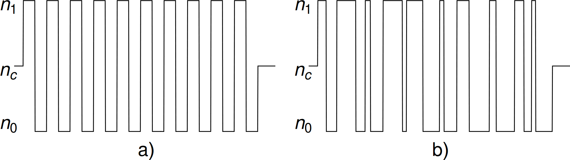
A quasi-1D ordered optical lattice waveguide can be realized by periodically stacking dielectric layers with different refractive indexes on top of each other. Fig. 1(a) shows the refractive index profile of a periodic quasi-1D optical waveguide where $n_{0}$, $n_{1}$, and $n_{c}$ correspond to the lower index layers, higher index layers, and cladding, respectively. We also define the refractive index contrast as $\Delta n=n_{1}-n_{0}$. In order to make a disordered waveguide, the thickness of the layers is randomized around an average value. We always assume that $n_{1}=1.50$ and $n_{c}=n_{0}$, while our simulations are carried out for either high contrast ($\Delta n=0.1$, $n_{0}=1.4$), or low contrast ($\Delta n=0.05$, $n_{0}=1.45$) . The total number of layers alternating in $n_{0}$ and $n_{1}$ in each sample waveguide is always 100, and the average thickness of each waveguide is $2\lambda$, where $\lambda$ is the optical wavelength at which the simulations are performed. The average thickness is chosen for maximum localization according to Ref. Mafi-Salman-Modal-JOSAB-2013 . The actual thickness of each layer is a random number $2\lambda+\Delta d$, where $\Delta d$ represents the variation in the thickness. $\Delta d$ is a random number that is chosen from a uniform random distribution of ${\rm unif}[-2r\lambda,2r\lambda]$. The amount of randomness is controlled by the $r$-parameter, $0\leq r\leq 1$; where $r=0$ corresponds to the periodic lattice. We refer to $r$ as the disorder strength. The waveguide is padded from each side with a layer of $5\lambda$ in thickness and refractive index of $n_{c}$. Fig. 1(b) shows a sketch of the refractive index profile of a quasi-1D disordered optical waveguide, where the number of layers are reduced for an easier visualization.

Note that because the total number of alternating layers is fixed at 100 but the thickness of each layer is random, the total width of the waveguide varies in each element of the random ensemble (each waveguide). The width variation ranges from zero to 5.6% for $0\leq r\leq 1$, respectively. Although a larger value of $r$ is associated with a larger variation in the width of the waveguide, it also results in a stronger confinement, hence making the calculations less dependent on the width of the waveguide Mafi-Behnam-Scaling-PRB-2016 . Therefore, the very same disorder that induces the waveguide width variation is responsible for Anderson localization, which makes the results of this paper independent of the width variation.

Figure 1: Sample refractive index profiles of (a) ordered and (b) disordered slab waveguides are shown.

In Fig. 2(a), we plot two guided modes of a quasi-1D periodic waveguide with the highest propagation constant. These two modes belong to a large group of standard extended Bloch periodic guided modes supported by the ordered optical waveguide, which are modulated by the overall mode profile of the quasi-1D waveguide Mafi-Salman-Modal-JOSAB-2013 . The total number of guided modes depends on the total thickness and the refractive index values of the slabs and cladding. The key point is that each mode of the periodic structure extends over the entire width of the waveguide structure. A similar exercise can be done with a quasi-1D disordered waveguide, where two arbitrarily selected modes are plotted in Fig. 2(b) using the same refractive index parameters as that of the periodic waveguide. It is clear that the modes become localized in the quasi-1D disordered waveguide. While there are variations in the shape and width of the modes, the mode profiles shown in Fig. 2(b) are typical.

Figure 2: Typical mode profiles for (a) an ordered slab waveguide where each mode extends over the entire waveguide, and (b) a disordered slab waveguide, where the modes are spatially localized.

III Mode group index PDF

The group index of mode $i$ is defined as the $n^{i}_{g}=c\beta^{(1)}_{i}$, where $c$ is the speed of light in vacuum. In Fig. 3, we plot the group index PDF for the periodic waveguide ($r=0.0$), and disordered waveguides with $r=0.25$, $r=0.50$, and $r=1.0$; with $\Delta n=0.1$. The area under each PDF curve integrates to unity, and each curve is generated using the statistical information from stimulating 6,000 waveguides, amounting to nearly 770,000 guided modes. The PDF of the periodic waveguide is highly peaked around $n_{g}\approx 1.5065$; however, there are also broad secondary peaks near $n_{g}\approx 1.520$ and $n_{g}\approx 1.485$. The modal patterns do not give any obvious clues on which category of mode shapes belong to which group-index bins. When a moderate amount of disorder with $r=0.25$ is introduced, the broad peak near $n_{g}\approx 1.485$ disappears, the main peak near $n_{g}\approx 1.520$ is lowered and broadened, while the peak around $n_{g}\approx 1.5065$ is raised. As the amount of disorder is further increased to $r=0.5$ and $r=1.0$, third and fourth peaks appear at larger values of group index, respectively.

Figure 3: Mode group index PDF for the periodic waveguide ($r=0.0$), and disordered waveguides with $r=0.25$, $r=0.50$, and $r=1.0$. Simulations are for the refractive index contrast of $\Delta n=0.1$ and the area under each PDF curve integrates to unity.

By looking at the general shapes of PDF curves in Fig. 3, one can claim that a higher level of disorder amounts to a broader PDF curve, i.e., the diversity in groups index values is increased. In other words, on average, a broader range of group velocities becomes accessible in the presence of increasing disorder. In order to further verify this claim, in Fig. 4, we repeat the simulations of Fig. 3, except for the lower refractive index contrast of $\Delta n=0.05$. In Fig. 4, the mode group index PDF related to $r=0.25$ appears to have the narrowest and highest form. Looking at Fig. 4, one can claim that there appears to be an optimal amount of disorder strength that narrows the range of group velocities and possibly reduces the pulse broadening. We will come back to these two seemingly contradictory conclusions in section IV, but for now we continue to look for other clues on the impact of disorder on the statistical behavior of group index in these waveguides.

Figure 4: Similar to Fig. 3, except for the refractive index contrast of $\Delta n=0.05$.

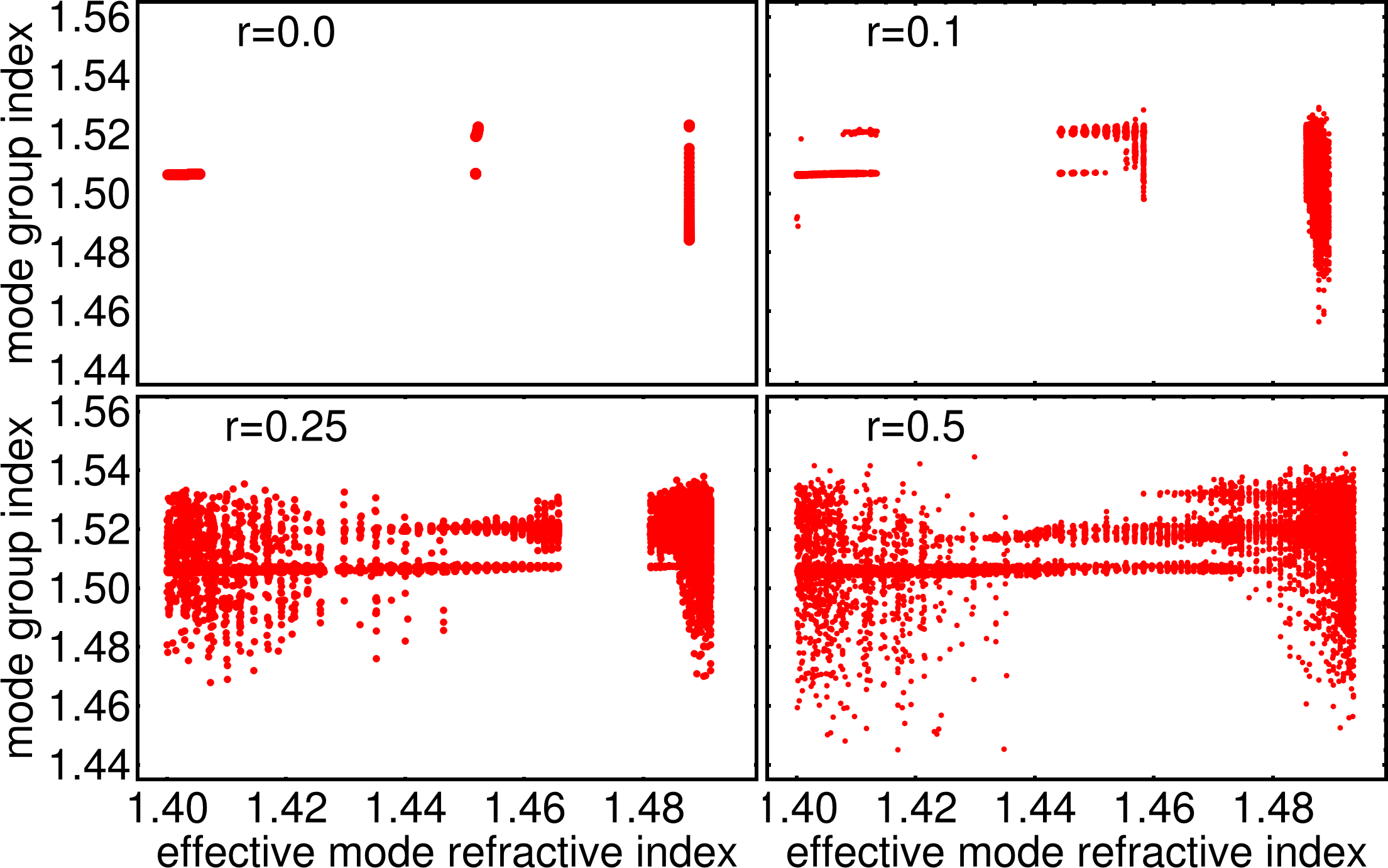
In Fig. 5 we present a scatter plot of the group index, $n_{g}$, versus the effective mode refractive index, $n_{p}=c\beta/\omega$, for each guided mode. The plots are presented again for $r=0.0$, $r=0.25$, $r=0.50$, and $r=1.0$, and each scatter plot is generated from stimulating 100 waveguides with the refractive index contrast of $\Delta n=0.1$. Note that for the periodic case of $r=0.0$, the result is always the same, because the waveguide refractive index profile is fully deterministic. For $r=0.0$, bandgaps in $n_{p}$ are observed and the range of $n_{g}$ is limited. As the disorder is introduced and gradually increased, the available range of both $n_{p}$ and $n_{g}$ are expanded and the gaps in $n_{g}$ eventually close. Again, the disorder increases the diversity in the values of both $n_{p}$ and $n_{g}$. We recall that the accessible values of $n_{p}$ in a waveguide are responsible for the shape of the spatial patterns, in addition to the modal intensity profiles. For example, if the values of $n_{g}$ are regularly spaced, the beam pattern in the waveguide repeats its shape periodically; e.g., in a graded-index optical fiber, this repetition happens with a sub-millimeter period as the beam propagates along the fiber Mafi:11 ; liu2016kerr ; wright2016self . For disordered waveguides where such an order is broken, pattern repetition is eliminated because of the large number of modes and random values of $n_{p}$. This behavior combined with the localized modal intensity profiles is responsible for the high quality of image transport through TALOFs. Similar comments can be made about the diversity in values of $n_{g}$ and its impact of the temporal shape of an optical pulse, which will be discussed in detail in section IV.

Figure 5: Scatter plot of the group index, $n_{g}$, versus the effective mode refractive index, $n_{p}=\beta/\omega$, for each guided mode. The plots are presented for $r=0.0$, $r=0.25$, $r=0.50$, and $r=1.0$. The refractive index contrast is $\Delta n=0.1$.

In order to further elaborate on the diversity of the $n_{g}$ values of the guided modes, in Fig. 6 we plot the values of $n_{g}$ for both the periodic waveguide with $r=0.0$ and the maximally disordered waveguide $r=1.0$. The refractive index contrast is assumed to be $\Delta n=0.1$ in this figure. In the left panel corresponding to $r=0.0$, we plot the values of $n_{g}$ versus the mode number (138 guided modes), where we have ordered the modes based on their $n_{g}$ values. In the right panel corresponding to $r=1.0$, we simulate 100 waveguides and show the $n_{g}$ values in an ascending order. The result shows that in a highly disordered waveguide, the group index values for the majority of the modes are still similar to those of a periodic waveguide with $r=0.0$; however, nearly 10%-20% of the modes exhibit strong deviations in group index and assume considerably smaller or larger values.

Figure 6: Values of the group index, $n_{g}$, versus the mode number for the periodic waveguide with $r=0.0$ and the maximally disordered waveguide $r=1.0$. For $r=1.0$, we simulate 100 waveguides and show the $n_{g}$ values in a ascending order. The refractive index contrast is $\Delta n=0.1$.

IV Pulse propagation and broadening

The results presented in Figs. 3 and 4 show the impact of the disorder strength and refractive index contrast on the group index distribution in these disordered waveguides. However, it may be hard to make a concrete conclusion about pulse broadening from such figures, especially because the results appear to be somewhat contradictory as explained in section III. The reason is that the pulse broadening is affected by the GV distribution of only those guided modes which are excited by the input pulse. For example, a typical input beam with a Gaussian spatial profile is likely to excite those modes which have less phase variations. As we explained in section III, we tried to look at the modal profiles to build a correlation between the profiles and GV values; however, it was inconclusive. As such, in this section, we resort to direct computation to evaluate the impact of the GV distribution of Figs. 3 and 4 on pulse width. The pulse width is important in setting the accessible communication bandwidth and is also essential for nonlinear properties of these waveguides.

In order to evaluate the pulse broadening, we assume that the in-coupling electric field is Gaussian in spatial profile, but is extremely narrow (Dirac delta function) in its temporal profile. The Gaussian spatial profile has a radius of $w=5$ µm, is centrally aligned with the waveguide, and is expressed as

$$\ket{W}=\Big{(}\dfrac{2}{\pi w^{2}}\Big{)}^{1/4}\exp{\left(-\dfrac{x^{2}}{w^{2}}\right)},$$ (3)

where $\braket{W}{W}=1$. The bra-ket notation indicates integration in the transverse $x$-coordinate. The guided modes in each waveguide are identified with $\ket{i}$ ($\braket{i}{i}=1$), where $i=1,\cdots,M$ is the mode index. For example, for $\Delta n=0.1$, there are approximately $M=140$ guided modes supported by the waveguide. For each waveguide, the modal excitation amplitudes are calculated as $c_{i}=\braket{i}{W}$ and the fractional power in each mode is given by $p_{i}=|c_{i}|^{2}$. The fractional power is nonzero mainly for those modes which are positioned near the center of the waveguide and have an overlap with $\ket{W}$. We define the coupling efficiency as $\eta=\sum^{M}_{i=1}p_{i}$, where $0\leq\eta\leq 1$. When $\eta<1$, which is almost always the case, some of the power does not couple to the guided modes and is radiated out. In order to calculate the pulse broadening due to the modal dispersion, we follow the procedure outlined in Ref. Pepeljugoski ; Mafi-bandwidth . The temporal profile of the input excitation is $\delta(t)$; however, as it couples into different modes that propagate with different GVs, the pulse breaks into multiple subpulses:

$$\delta(t)\to\sum^{M}_{i=1}p_{i}\delta(t-\tau_{i}),$$ (4)

where $\tau_{i}=n^{i}_{g}L/c$ is the modal delay for mode $\ket{i}$, $n^{i}_{g}$ is the group index of mode $\ket{i}$, $L$ is the propagation length, and $c$ is the speed of light in vacuum. The pulse broadening, $\delta\tau$, is calculated using

$$(\delta\tau)^{2}=2\eta^{-1}\sum^{M}_{i=1}p_{i}(\tau_{i}-\bar{\tau})^{2},$$ (5)

where $\bar{\tau}$ is the temporal center of the broken (broadened) pulse given by

$$\bar{\tau}=\eta^{-1}\sum^{M}_{i=1}p_{i}\tau_{i}.$$ (6)

In Fig. 7, we plot the coupling efficiency, $\eta$, as a function of the disorder strength for the two cases of $\Delta n=0.1$ and $\Delta n=0.05$. For each data point, we have simulated 1,000 waveguides and calculated the value of $\eta$ for each waveguide; the dark circle shows the mean value of $\eta$ averaged over the 1,000 waveguides and the error-bar indicates one standard deviation around the mean value. Of course, $\eta$ is generally higher for $\Delta n=0.1$ than $\Delta n=0.05$, because a larger number of guided modes are supported in the former case. This result is important because it shows that in coupling to a typical disordered waveguide, on average, only 70%-80% of the power can be coupled in and the rest is radiated out. In Fig. 8, we show the pulse broadening per unit length, $\delta\tau/L$, as a function of the disorder strength for two cases of $\Delta n=0.1$ and $\Delta n=0.05$. Again, the results are averaged over the 1,000 waveguides for each data point. These figures indicate that a small amount of disorder, typically around $r\approx 0.1-0.15$, achieves minimal pulse broadening compared to the case of no-disorder or highly disordered waveguides.

Figure 7: The coupling efficiency is plotted as a function of the disorder strength for two cases of $\Delta n=0.1$ and $\Delta n=0.05$. Each data point is averaged over 1,000 waveguides and the error-bar indicates one standard deviation around the mean value.

Figure 8: Pulse broadening per unit length is plotted as a function of the disorder strength for two cases of $\Delta n=0.1$ and $\Delta n=0.05$. Each data point is averaged over 1,000 waveguides and the error-bar indicates one standard deviation around the mean value.

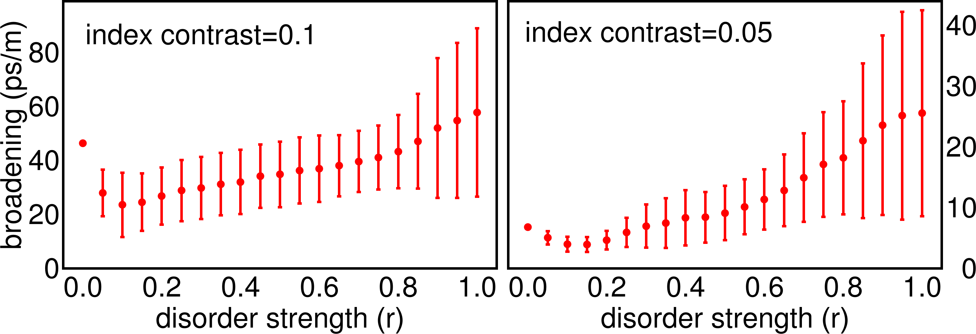
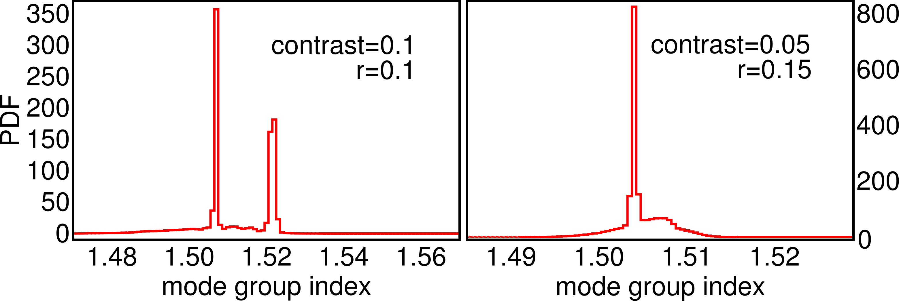
The data from Fig. 8 indicates an optimal disorder value to achieve a minimal amount of pulse broadening. Equipped with this information, we can now go back to the discussion surrounding Figs. 3 and 4 in section III. We recall that Fig. 3 indicated that a higher level of disorder amounts to a broader range of group velocities, while Fig. 4 indicated an optimal value for the disorder strength. In order to address this issue, in Fig. 9, we plot the mode group index PDFs at $r=0.1$ for $\Delta n=0.1$ and $r=0.15$ for $\Delta n=0.05$, respectively. These values correspond to the minima of the pulse broadening curves in Fig. 8. By comparing Fig. 9 and Fig. 4, it can be clearly seen that for $\Delta n=0.05$, $r=0.15$ provides the narrowest and tallest PDF curve, which is clearly consistent with the results reported in Fig. 8. For $\Delta n=0.1$, by comparing Fig. 9 and Fig. 3, in particular comparing $r=0.1$ and $r=0.0$, it can be observed that both the primary peak at $n_{g}\approx 1.5065$ and the secondary peak at $n_{g}\approx 1.520$ narrow down considerably for $r=0.1$ and the mode group index values below the primary peak disappear for $r=0.1$. As such, both results confirm the presence of an optimal value in the disorder strength to achieve the minimum pulse broadening.

Figure 9: Similar to Fig. 3, except for $\Delta n=0.1$ and $r=0.1$ in the left panel and $\Delta n=0.05$ and $r=0.15$ in the right panel.

It must be noted that although the input pulse is assumed to be extremely narrow, i.e., a Dirac delta function, the same results would be readily obtained with a longer input pulse. The choice of a Dirac delta function is merely a matter of convenience. In other words, for a Gaussian input pulse of temporal width $\tau_{\rm in}$, which broadens to $\tau_{\rm out}$ upon propagation through the waveguide, it can be shown that $\delta\tau=(\tau^{2}_{\rm out}-\tau^{2}_{\rm in})^{1/2}$, where $\delta\tau$ is independent of $\tau_{\rm in}$. Therefore, the same value of pulse broadening is obtained from a broader Gaussian pulse as from a Dirac delta function. Note that this statement does not strictly hold if the second or higher order dispersive effects are taken into account, all of which are of higher-order-contribution and play a less important role in the pulse broadening in normal circumstances.

IV.1 Metric for pulse broadening using the PDF curves

In light of the observations in Fig. 8 and how they relate to Figs. 3, 4, and 9, we define a metric to assess the width of the PDF curves; the goal is to establish a relationship between this metric and the the pulse broadening values in Fig. 8. A metric, at the minimum, should be able to predict the optimal of the disorder strength for minimal pulse broadening. We use the square of the inverse population ratio (IPR) of the PDF curves as the metric. The IPR is defined as:

$${\rm IPR}=\int\big{[}\rm PDF(n_{g})\big{]}^{2}\,dn_{g},$$ (7)

where ${\rm PDF}(n_{g})$ represents any of the PDF curves in Figs. 3, 4, and 9. Note that unlike the commonly used 4th power in the definition of IPR (see, e.g., Ref. PhysRevLett.105.183901 ), we only use the 2nd power of PDF in Eq. 7: the reason is that the PDF is a non-negative probability density function and is similar to $|\psi|^{2}$, if $\psi$ is regarded as the (quantum-mechanical) wave amplitude. We recall that the area under each PDF curve integrates to unity: $\int{\rm PDF}(n_{g})\,dn_{g}=1$. In Fig. 10, we plot the metric, i.e. ${\rm IPR^{2}}$ as a function of the disorder strength, both for $\Delta n=0.1$ and $\Delta n=0.05$. Fig. 10 should be compared with Fig. 8; the disorder contrast corresponding to the minimum pulse broadening is almost exactly predicted by the metric. Moreover, the correlation factor between the metric and the mean values presented in Fig. 10 is 89% for $\Delta n=0.1$ and 99% for $\Delta n=0.05$. Therefore, the ${\rm IPR^{2}}$ metric appears to be a powerful tool that can predict the pulse broadening performance of such disordered waveguides directly using the PDF curves and without resorting to specific pulse propagation simulations.

Figure 10: The ${\rm IPR^{2}}$ metric is calculated from the PDF curves as a function of the disorder contrast ($r$) for both $\Delta n=0.1$ and $\Delta n=0.05$. Each PDF curve is obtained by simulating 1,000 waveguides.

V Mode group index PDF versus localization length

We discussed earlier that the presence of disorder results in the TAL of the guided modes. Therefore, as the disorder strength is increased, on average, the modes should become smaller in width. In this section, we explore the correlation between the localization width of the guided modes and their group index. For each guided mode, the mode width $\mathcal{W}$ is defined based on the standard deviation $\sigma$ of the (1D) normalized intensity distribution $I(x)\propto|A(x)|^{2}$ of the mode according to

$$\sigma^{2}=\int_{-\infty}^{+\infty}~{}(x-\bar{x})^{2}~{}I(x)~{}dx,$$ (8)

where we define the mode center as

$$\bar{x} =\int_{-\infty}^{+\infty}x~{}I(x)~{}dx.$$ (9)

$x$ is the spatial coordinate across the width of the waveguide and the mode intensity profile is normalized such that $\int_{-\infty}^{+\infty}I(x)dx=1$. We define $\mathcal{W}=\sqrt{2}\sigma$ as a measure of the width of the modes, i.e. a larger $\mathcal{W}$ signifies a wider mode intensity profile distribution.

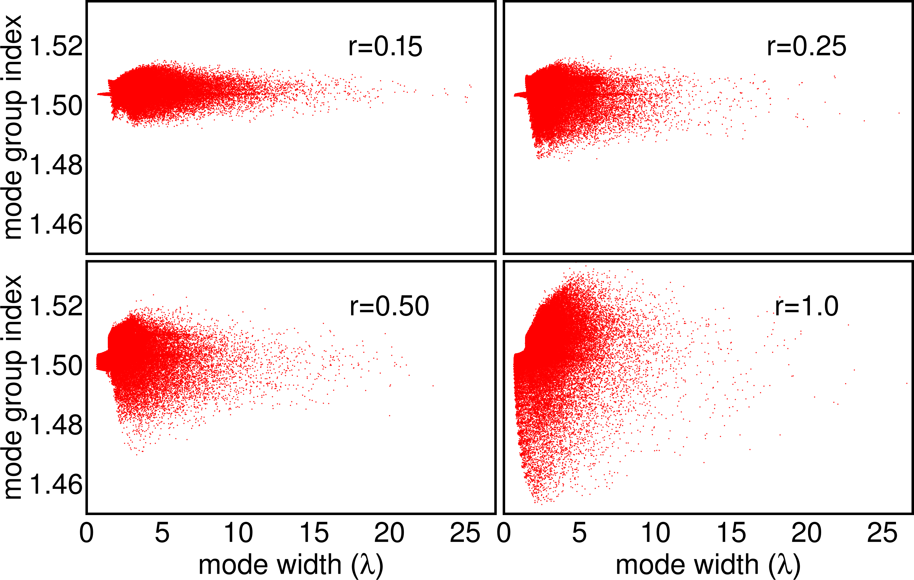
In Fig. 11, we present a scatter plot of the group index, $n_{g}$, versus the mode width, $\mathcal{W}$, for each guided mode. The plots are presented for $r=0.1$, $r=0.25$, $r=0.50$, and $r=1.0$, while the refractive index contrast is assumed to be $\Delta n=0.1$. We note that $r=0.1$ corresponds to the minimum pulse spreading for $\Delta n=0.1$ according to the left panel in Fig. 8. Similarly, in Fig. 12, we present a scatter plot of the group index, $n_{g}$, versus the mode width, $\mathcal{W}$, for each guided mode. The plots are presented for $r=0.15$, $r=0.25$, $r=0.50$, and $r=1.0$, while the refractive index contrast is assumed to be $\Delta n=0.05$. We note that $r=0.15$ corresponds to minimum pulse spreading for $\Delta n=0.05$ according to the right panel in Fig. 8. The data in each subfigure is generated from the simulation of 1,000 independent waveguides resulting in 138,000 modes. We note that the lowest value of $r$ in each figure corresponds to the narrowest group index distribution and the widest mode-width distribution. As the disorder is increased, the group index distribution increases, while the mode-width distribution decreases. This observation is consistent with the TAL behavior is disordered waveguides and our discussions on group index distribution in previous sections.

Figure 11: Scatter plot of the group index, $n_{g}$, versus the mode width, $\mathcal{W}$, for each guided mode. The plots are presented for $r=0.1$, $r=0.25$, $r=0.50$, and $r=1.0$. The refractive index contrast is $\Delta n=0.1$.

Figure 12: Scatter plot of the group index, $n_{g}$, versus the mode width, $\mathcal{W}$, for each guided mode. The plots are presented for $r=0.15$, $r=0.25$, $r=0.50$, and $r=1.0$. The refractive index contrast is $\Delta n=0.05$.

VI conclusion

In this manuscript, we have introduced the mode group index PDF as a powerful tool to study the dispersion properties of guided modes in a disordered quasi-1D slab optical waveguide. We observe that the minimum amount of modal dispersion corresponds to a small amount of disorder, i.e., no disorder or large disorder both result in a large modal dispersion. We establish a metric that is applied to the mode group index PDF and can reliably predict the optimal amount of disorder for a minimal pulse dispersion. The metric is a measure of the width of the PDF and its value is strongly correlated with the modal dispersion of a pulse propagating in the disordered waveguide. While the simulations are for a certain class of disordered quasi-1D waveguides, they appear to conform well with the physical intuition and are likely to hold in other designs. The results presented in the manuscript are intended to establish the framework for a comprehensive analysis of the group velocity statistics for quasi-2D transverse Anderson localization in disordered optical fibers in the future.

It is quite plausible to expect that in a transversely disordered optical fiber, similar to the disordered quasi-1D slab optical waveguide, the minimum amount of modal dispersion corresponds to an optimal (and likely a small) amount of disorder. While a longitudinally invariant and transversely disordered optical fiber is not inherently more lossy than a conventional core-cladding optical fiber, it is likely to be fabricated by a method that is more prone to manufacturing uncertainties, such as the stack-and-draw method Mafi-Salman-OL-2012 . Such manufacturing uncertainties can break the longitudinal invariance and result in attenuation, as well as polarization coupling. The undesirable attenuation must be addressed in a case-by-case basis by making better fibers or amplifying the signal. Pulse broadening due to the random polarization coupling is likely going to be negligible compared to the modal dispersion, similar to a conventional optical fiber; however, this issue warrants further research.

References

- (1) S. S. Abdullaev, F. K. Abdullaev, On propagation of light in fiber bundles with random parameters, Radiofizika 23 (6) (1980) 766–767.
- (2) H. De Raedt, A. Lagendijk, P. de Vries, Transverse localization of light, Phys. Rev. Lett. 62 (1) (1989) 47–50.
- (3) P. W. Anderson, Absence of diffusion in certain random lattices, Phys. Rev. 109 (5) (1958) 1492–1505.
- (4) P. W. Anderson, D. J. Thouless, E. Abrahams, D. S. Fisher, New method for a scaling theory of localization, Phys. Rev. B 22 (8) (1980) 3519–3526.
- (5) E. Abrahams, 50 years of Anderson Localization, World Scientific, Singapore, 2010.
- (6) A. Lagendijk, B. van Tiggelen, D. S. Wiersma, Fifty-years of Anderson localization, Physics Today 62 (8) (2009) 24–29.
- (7) E. Abrahams, P. W. Anderson, D. C. Licciardello, T. V. Ramakrishnan, Scaling theory of localization: Absence of quantum diffusion in two dimensions, Phys. Rev. Lett. 42 (10) (1979) 673–676.
- (8) A. D. Stone, J. D. Joannopoulos, Probability distribution and new scaling law for the resistance of a one-dimensional Anderson model, Phys. Rev. B 24 (6) (1981) 3592–3595.
- (9) P. Sheng, Introduction to wave scattering, localization and mesoscopic phenomena, 2nd Edition, Springer-Verlag, Berlin, Germany, 2006.
- (10) T. Schwartz, G. Bartal, S. Fishman, M. Segev, Transport and Anderson localization in disordered two-dimensional photonic lattices, Nature 446 (7131) (2007) 52–55.
- (11) Y. Lahini, A. Avidan, F. Pozzi, M. Sorel, R. Morandotti, D. N. Christodoulides, Y. Silberberg, Anderson localization and nonlinearity in one-dimensional disordered photonic lattices, Phys. Rev. Lett. 100 (1) (2008) 013906.
- (12) L. Martin, G. D. Giuseppe, A. Perez-Leija, R. Keil, F. Dreisow, M. Heinrich, S. Nolte, A. Szameit, A. F. Abouraddy, D. N. Christodoulides, B. E. A. Saleh, Anderson localization in optical waveguide arrays with off-diagonal coupling disorder, Opt. Express 19 (14) (2011) 13636–13646.
- (13) S. Karbasi, C. R. Mirr, P. G. Yarandi, R. J. Frazier, K. W. Koch, A. Mafi, Observation of transverse Anderson localization in an optical fiber, Opt. Lett. 37 (12) (2012) 2304–2306.
- (14) S. Karbasi, C. R. Mirr, R. J. Frazier, P. G. Yarandi, K. W. Koch, A. Mafi, Detailed investigation of the impact of the fiber design parameters on the transverse Anderson localization of light in disordered optical fibers, Opt. Express 20 (17) (2012) 18692–18706.
- (15) S. Karbasi, T. Hawkins, J. Ballato, K. W. Koch, A. Mafi, Transverse Anderson localization in a disordered glass optical fiber, Opt. Mater. Express 2 (11) (2012) 1496–1503.
- (16) Y. Silberberg, M. Segev, D. N. Christodoulides, Anderson localization of light, Nat. Photonics 7 (3) (2013) 197–204.
- (17) A. Mafi, Transverse Anderson localization of light: a tutorial, Adv. Opt. Photon. 7 (3) (2015) 459–515.
- (18) E. Fratini, S. Pilati, Anderson localization in optical lattices with correlated disorder, Phys. Rev. A 92 (6) (2015) 063621.
- (19) X. Yao, X. Liu, Beam dynamics in disordered p t-symmetric optical lattices based on eigenstate analyses, Phys. Rev. A 95 (3) (2017) 033804.
- (20) H. Yılmaz, C. W. Hsu, A. Yamilov, H. Cao, Transverse localization of transmission eigenchannels, Nat. Photonics 13 (5) (2019) 352.
- (21) J. Guglielmon, M. C. Rechtsman, Inducing maximal localization with fractal waveguide arrays, Phys. Rev. A 99 (2019) 063807.
- (22) S. Karbasi, R. J. Frazier, K. W. Koch, T. Hawkins, J. Ballato, A. Mafi, Image transport through a disordered optical fibre mediated by transverse Anderson localization, Nat. Commun. 5 (3362) (2014).
- (23) T. H. Tuan, S. Kuroyanagi, K. Nagasaka, T. Suzuki, Y. Ohishi, Near-infrared optical image transport through an all-solid tellurite optical glass rod with transversely-disordered refractive index profile, Opt. Express 26 (13) (2018) 16054–16062.
- (24) H. T. Tong, S. Kuroyanagi, K. Nagasaka, T. Suzuki, Y. Ohishi, Characterization of an all-solid disordered tellurite glass optical fiber and its near-infrared optical image transport, Jpn. J. Appl. Phys (2018).
- (25) J. Zhao, J. E. A. Lopez, Z. Zhu, D. Zheng, S. Pang, R. A. Correa, A. Schülzgen, Image transport through meter-long randomly disordered silica-air optical fiber, Sci. Rep. 8 (1) (2018) 3065.
- (26) J. Zhao, Y. Sun, Z. Zhu, J. E. Antonio-Lopez, R. A. Correa, S. Pang, A. Schülzgen, Deep learning imaging through fully-flexible glass-air disordered fiber, ACS Photonics 5 (10) (2018) 3930–3935.
- (27) S. Karbasi, K. W. Koch, A. Mafi, Multiple-beam propagation in an Anderson localized optical fiber, Opt. Express 21 (1) (2013) 305–313.
- (28) G. Ruocco, B. Abaie, W. Schirmacher, A. Mafi, M. Leonetti, Disorder-induced single-mode transmission, Nat. Commun. 8 (14571) (2017).
- (29) M. Leonetti, S. Karbasi, A. Mafi, C. Conti, Light focusing in the Anderson regime, Nat. Commun. 5 (4534) (2014).
- (30) B. Abaie, M. Peysokhan, J. Zhao, J. E. Antonio-Lopez, R. Amezcua-Correa, A. Schülzgen, A. Mafi, Disorder-induced high-quality wavefront in an Anderson localizing optical fiber, Optica 5 (8) (2018) 984–987.
- (31) Leonetti, Marco and Karbasi, Salman and Mafi, Arash and Conti, Claudio, Experimental observation of disorder induced self-focusing in optical fibers, Appl. Phys. Lett. 105 (17) (2014) 171102.
- (32) M. Leonetti, S. Karbasi, A. Mafi, C. Conti, Observation of migrating transverse Anderson localizations of light in nonlocal media, Phys. Rev. Lett. 112 (19) (2014) 193902.
- (33) M. Leonetti, S. Karbasi, A. Mafi, E. DelRe, C. Conti, Secure information transport by transverse localization of light, Sci. Rep. 6 (29918) (2016).
- (34) S. Liang, Y. Zhang, X. Wang, X. Sheng, S. Lou, B. Lin, M. Dong, L. Zhu, Surface brillouin scattering in disordered optical fibers with transverse anderson localization guiding mechanism for evaluation of longitudinal structural fluctuations, IEEE Photonics Journal 10 (1) (2018) 1–8.
- (35) B. Abaie, E. Mobini, S. Karbasi, T. Hawkins, J. Ballato, A. Mafi, Random lasing in an Anderson localizing optical fiber, Light Sci. Appl. 6 (e17041).
- (36) K. Joshi, R. Kumar, M. Balasubrahmaniyam, S. Mujumdar, Effect of critical disorder on lifetime distributions of anderson-localized lasing modes, Phys. Rev. A 100 (2) (2019) 023803.
- (37) K. Okamoto, Fundamentals of Optical Waveguides, 2nd Edition, Academic Press, London, UK, 2006.
- (38) D. Gloge, E. Marcatili, Multimode theory of graded-core fibers, Bell Labs Tech. J. 52 (9) (1973) 1563–1578.
- (39) M. D. Feit, J. A. Fleck, Light propagation in graded-index optical fibers, Appl. Opt. 17 (24) (1978) 3990–3998.
- (40) V. Jolivet, P. Bourdon, B. Bennal, L. Lombard, D. Goular, E. Pourtal, G. Canat, Y. Jaouen, B. Moreau, O. Vasseur, Beam shaping of single-mode and multimode fiber amplifier arrays for propagation through atmospheric turbulence, IEEE Journal of Selected Topics in Quantum Electronics 15 (2) (2009) 257–268.
- (41) T. Čižmár, K. Dholakia, Exploiting multimode waveguides for pure fibre-based imaging, Nat. Commun. 3 (2012) 1027.
- (42) I. N. Papadopoulos, S. Farahi, C. Moser, D. Psaltis, High-resolution, lensless endoscope based on digital scanning through a multimode optical fiber, Biomedical optics express 4 (2) (2013) 260–270.
- (43) L. V. Amitonova, A. Descloux, J. Petschulat, M. H. Frosz, G. Ahmed, F. Babic, X. Jiang, A. P. Mosk, P. S. J. Russell, P. W. Pinkse, High-resolution wavefront shaping with a photonic crystal fiber for multimode fiber imaging, Opt. Lett. 41 (3) (2016) 497–500.
- (44) X. Zhu, A. Schülzgen, H. Li, H. Wei, J. V. Moloney, N. Peyghambarian, Coherent beam transformations using multimode waveguides, Opt. Express 18 (7) (2010) 7506–7520.
- (45) S. Karbasi, K. W. Koch, A. Mafi, Modal perspective on the transverse Anderson localization of light in disordered optical lattices, J. Opt. Soc. Am. B 30 (6) (2013) 1452–1461.
- (46) B. Abaie, A. Mafi, Scaling analysis of transverse Anderson localization in a disordered optical waveguide, Phys. Rev. B 94 (6) (2016) 064201.
- (47) B. Abaie and A. Mafi, Modal area statistics for transverse Anderson localization in disordered optical fibers, Opt. Lett. 43 (16) (2018) 3834–3837.
- (48) G. P. Agrawal, Nonlinear fiber optics, 5th Edition, Academic Press, 2013.
- (49) G. P. Agrawal, Fiber-optic communication systems, 4th Edition, John Wiley & Sons, 2012.
- (50) R. Stolen, J. Bjorkholm, A. Ashkin, Phase-matched three-wave mixing in silica fiber optical waveguides, Applied Physics Letters 24 (7) (1974) 308–310.
- (51) C. Lin, M. Bösch, Large-stokes-shift stimulated four-photon mixing in optical fibers, Applied Physics Letters 38 (7) (1981) 479–481.
- (52) K. Hill, D. Johnson, B. Kawasaki, Efficient conversion of light over a wide spectral range by four-photon mixing in a multimode graded-index fiber, Applied optics 20 (6) (1981) 1075–1079.
- (53) H. Pourbeyram, E. Nazemosadat, A. Mafi, Detailed investigation of intermodal four-wave mixing in smf-28: blue-red generation from green, Opt. Express 23 (11) (2015) 14487–14500.
- (54) E. Nazemosadat, A. Mafi, Nonlinear multimodal interference and saturable absorption using a short graded-index multimode optical fiber, J. Opt. Soc. Am. B 30 (5) (2013) 1357–1367.
- (55) D. Gloge, Impulse response of clad optical multimode fibers, Bell Labs Tech. J. 52 (6) (1973) 801–816.
- (56) S. Fan, J. M. Kahn, Principal modes in multimode waveguides, Opt. Lett. 30 (2) (2005) 135–137.
- (57) R. Olshansky, D. B. Keck, Pulse broadening in graded-index optical fibers, Appl. Opt. 15 (2) (1976) 483–491.
- (58) Y. Koike, T. Ishigure, E. Nihei, High-bandwidth graded-index polymer optical fiber, J. Light. Technol. 13 (7) (1995) 1475–1489.
- (59) Z. Zhu, L. G. Wright, D. N. Christodoulides, F. W. Wise, Observation of multimode solitons in few-mode fiber, Opt. Lett. 41 (20) (2016) 4819–4822.
- (60) W. H. Renninger, F. W. Wise, Optical solitons in graded-index multimode fibres, Nat. Commun. 4 (2013) 1719.
- (61) Spatiotemporal solitons in inhomogeneous nonlinear media, Opt. Commun. 180 (4) (2000) 377 – 382.
- (62) A. E. Vasdekis, G. E. Town, G. A. Turnbull, I. D. W. Samuel, Fluidic fibre dye lasers, Opt. Express 15 (7) (2007) 3962–3967.
- (63) E. Mobini, B. Abaie, M. Peysokhan, A. Mafi, Spectral selectivity in optical fiber capillary dye lasers, Opt. Lett. 42 (9) (2017) 1784–1787.
- (64) K.-P. Ho, J. M. Kahn, Statistics of group delays in multimode fiber with strong mode coupling, J. Light. Technol. 29 (21) (2011) 3119–3128.
- (65) B. Abaie, S. R. Hosseini, S. Karbasi, A. Mafi, Modal analysis of the impact of the boundaries on transverse Anderson localization in a one-dimensional disordered optical lattice, Opt. Comm. 365 (2016) 208–214.
- (66) R. G. S. El-Dardiry, S. Faez, A. Lagendijk, Snapshots of Anderson localization beyond the ensemble average, Phys. Rev. B 86 (12) (2012) 125132.
- (67) Y. V. Kartashov, V. V. Konotop, V. A. Vysloukh, L. Torner, Light localization in nonuniformly randomized lattices, Opt. Lett. 37 (3) (2012) 286–288.
- (68) T. A. Lenahan, Calculation of modes in an optical fiber using the finite element method and eispack, Bell Labs Tech. J. 62 (9) (1983) 2663–2694.
- (69) A. Mafi, P. Hofmann, C. J. Salvin, A. Schülzgen, Low-loss coupling between two single-mode optical fibers with different mode-field diameters using a graded-index multimode optical fiber, Opt. Lett. 36 (18) (2011) 3596–3598.
- (70) Z. Liu, L. G. Wright, D. N. Christodoulides, F. W. Wise, Kerr self-cleaning of femtosecond-pulsed beams in graded-index multimode fiber, Opt. Lett. 41 (16) (2016) 3675–3678.
- (71) L. G. Wright, Z. Liu, D. A. Nolan, M.-J. Li, D. N. Christodoulides, F. W. Wise, Self-organized instability in graded-index multimode fibres, Nat. Photonics 10 (12) (2016) 771.
- (72) P. Pepeljugoski, S. E. Golowich, A. J. Ritger, P. Kolesar, A. Risteski, Modeling and simulation of next-generation multimode fiber links, J. Light. Technol. 21 (5) (2003) 1242–1255.
- (73) A. Mafi, Bandwidth improvement in multimode optical fibers via scattering from core inclusions, J. Light. Technol. 28 (10) (2010) 1547–1555.
- (74) V. Krachmalnicoff, E. Castanié, Y. De Wilde, R. Carminati, Fluctuations of the local density of states probe localized surface plasmons on disordered metal films, Phys. Rev. Lett. 105 (2010) 183901.