Inverse Graphical Method for Global Optimization and Application to Design Centering Problem

Abstract

Consider the problem of finding an optimal value of some objective functional subject to constraints over numerical domain. This type of problem arises frequently in practical engineering tasks. Nowdays almost all general methods for solving such a problem are based on user-supplied routines computing the objective value at some points. We study another approach called inverse relying on some procedure to estimate the set of points instead having objective values bounded by a specified constant.

In particular, we present an inverse optimization algorithm derived from the bisection of the objective range. In case of seeking a proven global optimal solution inherently requiring many computations, and a problem with some kind of coherency utilized in estimation procedure, the inverse scheme is much more efficient than conventional ones. An example of such a problem, namely the design centering, is studied to compare the approaches.

1 Introduction

The numerical global optimization problems are of big importance for science, economics and technology. They are studied extensively for decades [15], [25], [32], [40]. We focus specifically on deterministic approaches, i.e. those leading to a proven result inevitably. The problem is usually formulated as follows:

$$\begin{gathered}f(x)\to\min\\ \mbox{s.t.}\;x\in F\subset X,\end{gathered}$$ (1)

where $f\colon X\to\mathbb{R}$ is an objective functional, $X$ is a problem domain and $F$ is some part of the domain called feasible region. The problem is constrained if $F\neq X$ and unconstrained otherwise. Restriction $x\in F$ is often formulated in terms of some equality or inequality constraints, but this is not necessarily. Note that in case of constant $f(x)$ the problem is called constraint satisfaction and there are plenty of methods solving this kind of problem.

According to the literature, it is almost always assumed in general optimization methods that we have some means to compute or bound $f(x)$ over specified subset $X^{\prime}\subset X$, and the solution algorithms are then based on such routines [32], [40], [34]. Custom algorithms are usually developed for particular explicit forms of objective and constraints [15], [23]. We hereafter call this conventional scheme straight. In this work we present an opposite approach to global optimization called inverse. It is based on computing domain subsets for specified objective bounds, see Fig. 1.

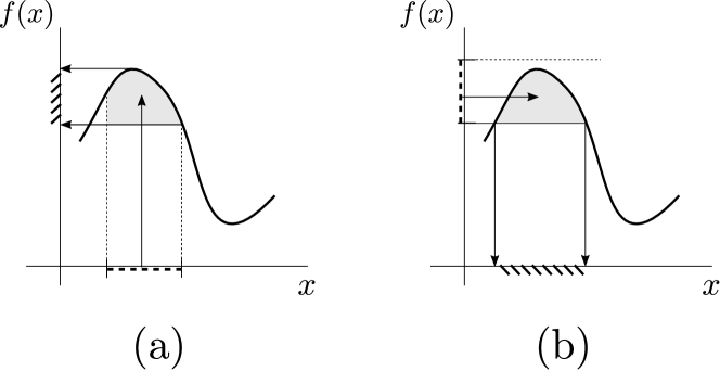
Figure 1: Computations within optimization: (a) straight(conventional), (b) inverse

Such framework is rather common in constraint satisfaction problems, but to the best of our knowledge no similar practical methods have been developed for optimization problems. It is worth noting that the performance of the new approach highly depends on a good domain estimation procedure provided for a particular problem. We present an example problem at the end of the article demonstrating a superiority of the inverse scheme while looking for a proven global optimal solution.

The rest of the article is organized as follows. We start with a brief review of the related research. Then we proceed to development of the inverse graphical method and proof of convergence. The second part of this work deals with a design centering problem arising in the diamond cutting industry. We discuss implementation details and compare the inverse approach to the state of the art technique as well as to the publicly available software libraries.

2 Related work

The closest optimization scheme so far has been pioneered by Sergey P. Shary [36] and studied in some works afterwards [1], [6]. We advance this study by switching entirely to inverse computations as shown in Fig. 1. This is done theoretically by stating sufficient convergency conditions and practically by developing complete algorithm for a specific problem. Note that although the works mentioned above deal with the algorthims in terms of equation solution, which can be thought of as a kind of inverse technique, the latter is still reduced to straight interval computations there. In practice this often means utilizing rather complex and expensive procedures. By contrast, the inverse scheme based on domain estimations could be implemented much simpler and faster for particular problems. Besides, we involve an inherently approximate computation framework providing more freedom to choose effective algorithms.

In addition to the above, we must note the following closely related research. The main idea of computing the domain region satisfying some restrictions is very common in constraint satisfaction study [28]. One notable example is the method based on the feasible region approximation with the help of spatial trees [31]. The inverse graphical method presented later in this article adapts similar ideas to the optimization problem. It can be thought of as a sequence of constraint satisfaction problems with added parametrized optimization constraint [11], [28]. More ideas on interchange between global optimization and constraint satisfaction can be found in [13], [14] and references therein.

Besides, the inverse optimization method can be thought of as a sequence of approximate problem solutions parametrized by the accuracy, or equivalently by the bounds on acceptable objective value. It is tightly connected to the successive approximation global optimization methods [16] as well as to the relief indicator method [39]. Compared to them the top-level algorithm scheme and the theoretical results are alike, but there are two differences of the new method. First, we connect tightly particular domain approximations and objective value boundaries. Precisely, we choose numerical approximations of the problem instead of adding new analytic constraints, and estimate feasible regions with the same tolerance as objective in contrast to accurate solving. Secondly, we involve easier graphical domain estimation technique at every iteration instead of constructing complex relaxations and underestimations [40]. These aspects together allow us to simplify the coarse steps of the overall algorithm and achieve a performance boost.

Furthermore, we can note non-complete optimization procedures called simulated annealing and threshold accepting [9]. They reduce the accuracy value as a parameter much like the inverse approach. However, these methods are non-deterministic, thus differ entirely from the subject of this article.

Now let us describe briefly the relations between the inverse scheme and conventional global optimization techniques. First, the inverse approach is in fact a numerical search of the optimal objective value. It is close to the well-known bisection method and its derivatives [43], but we bisect only on the objective range and use the domain estimation as a decision value. Comparing to the common branch-and-bound technique [32] the difference is the same: we subdivide(”branch”) the objective value range and estimate(”bound”) the domain instead of subdividing the domain and estimating the objective. Secondly, our approach can be treated as the opposite to the penalty function method [25] incorporating the constraints into the objective function. In contrast, we incorporate the bounded objective value as a new constraint and search for feasible points at every iteration of the inverse method.

At last, all the references concerning the design centering problem and the practical application of the inverse scheme are discussed in the second part of the article.

3 General inverse graphical optimization method

This section deals with the basic study of the inverse method. We will first proceed through the algorithm and then move to the proof of its convergence.

We derive the inverse graphical optimization method from the bisection methods [36],[43],[1]. In particular, we split the infinite objective range by some threshold value and then eliminate a part of it at every step of the algorithm. The elimination is done through the estimation of the domain region having objective values within the given range. With the objective value restricted to a range the problem transforms to the constraint satisfaction one and is solved by approximate procedures similarly to [31]. The global optimal solution is then acquired reducing the objective range while ensuring that the corresponding feasible region is not empty. Refer to Fig. 2 for general scheme.

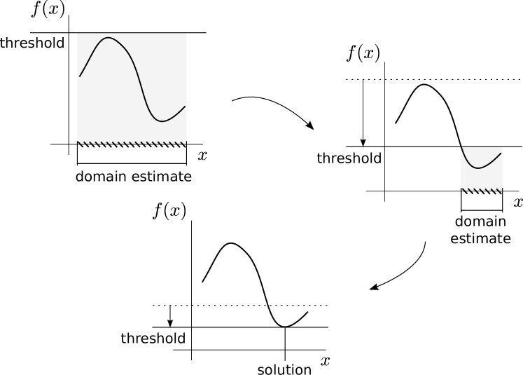
Figure 2: General scheme of the inverse optimization technique

Note that the core part of the inverse method is a domain estimation procedure applied at every step. One could imagine many possible variants, but we describe a specific one leaving the rest to the further research. Precisely, we approximate the domain by equally-sized hyperrectangles and then mark them according to the objective values. This approach is very close to the raster computer graphics. Moreover, we use some rasterization techniques in the application. Thus we call our variant of the inverse method graphical.

Let us formalize the problem to solve. In this article we consider the following optimization problem:

$$\begin{gathered}f(x)\to\min\\ \mbox{s.t.}\;x\in F\subset X\end{gathered}$$ (2)

where $f\colon X\to\mathbb{R}$ is a continuous function, $X=[x_{1}^{L},x_{1}^{R}]\times[x_{2}^{L},x_{2}^{R}]\times\cdots\times[x_{n}^{L},x_{n}^{R}]\subset\mathbb{R}^{n}$ is a compact hyperrectangle in Euclidean space and $F\subset X$ is a closed region called the feasible region. As a restriction of our study we additionally assume that the feasible region contains an interior point, this also leads to existence of the solution. Note that in practice one could take the feasible region bounding box as $X$.

In the rest of the article by $\mathcal{B}$ we denote the set of all hyperrectangles in $\mathbb{R}^{n}$ and any $B\in\mathcal{B}$ we call simply a box. Note that all the boxes are closed sets. For any $B\in\mathcal{B}$ by $\delta(B)$ we denote the diameter of $B$ as a set, i.e. the maximum distance between points in $B$. For any set $S\subset\mathbb{R}^{n}$ by $\mathop{\mathrm{int}}\nolimits(S)$ we denote the interior of $S$ and by $\partial S$ we denote the boundary of $S$.

3.1 The algorithm

Now we develop the inverse graphical optimization algorithm. Consider a problem of form (2) and a target accuracy $\varepsilon>0$ for the solution. The key feature of the algorithm is the assumption that we have a domain estimation procedure for a particular problem. By the domain estimation procedure we consider some algorithm to compute a relation

$$C\colon\mathcal{B}\times\mathbb{R}\to\{0,\beta,1\}$$

such that for any box $B\in\mathcal{B}$ and threshold $t\in\mathbb{R}$

$$C(B,t) =0\mbox{ only if for all $x\in B$ $x\not\in F$ or $f(x)>t$},$$

$$C(B,t) =1\mbox{ only if for all $x\in B$ $x\in F$ and $f(x)\leq t$},$$

$$C(B,t) =\beta\mbox{ in any other or unknown case}.$$

According to this for a given threshold $t$ we call the box $B$ empty if $C(B,t)=0$, filled if $C(B,t)=1$ and boundary if $C(B,t)=\beta$. For more insights on such a procedure, see [31]: our empty, boundary and filled boxes roughly correspond to the black, grey and white ones in [31]. Some ideas on constructing the practical domain estimation procedure can be found in [30] and we provide some research for a different problem in the second part of the article. Note that any filled box lies completely inside the feasible region. Moreover, we emphasize that any actually empty or filled box in general can be labeled as boundary by our definition of the procedure, which is not the case in [30],[31].

Intuitively these notions represent the fact that when we seek for solutions to (2) with the objective value of $t$ or better. Thus, box $B$ is empty if there are no such points in it and $B$ is filled if any point of $B$ constitute such a solution. The boundary boxes represent the area of uncertainty of either the problem or the algorithm. The uncertainties of the problem are the boxes with objective values on both sides of threshold $t$ or both feasible and infeasible. The algorithm uncertainties may come from the approximating techniques, for example when precise domain estimation needs a lot of computational resources and we consider some rough but faster algorithm. We state some sufficient conditions on the choice of the algorithms to ensure the convergence of the method.

To continue developing, assume a given parameter $S$ of the algorithm called domain scale. This parameter controls the balance between domain regions sizes and objective values at iteration steps. It seems that $S$ should be connected to the Lipschitz constant of objective, but this question have not been studied yet. As a rule of thumb, $S=0.6$ performed well enough for the design centering problems tested in the second part of the work. The theoretical results do not depend on the value of $S$ as well.

With all the definitions above the inverse graphical optimization algorithm is defined as follows.

 

The inverse graphical optimization algorithm

1. Let $\mathcal{X}$ be the set of active boxes in the algorithm, $\delta$ be the current accuracy, and $t$ be the current objective threshold for the problem. Assume that an initial value of $t$ satisfying

   $$t>\min_{F}f(x)$$

   is somehow known from the problem domain, see notes below for details. Initialize $\mathcal{X}=\{X\}$ and $\delta=S\delta(X)$ where $X\in\mathcal{B}$ is any box containing the feasible region and $S$ is the domain scale parameter of the algorithm.

2. Find the tight approximate threshold for the problem as follows.

   1. Compute $C(X_{i},t-\delta)$ for every $X_{i}\in\mathcal{X}$ by applying the domain estimation procedure.

   2. If there exists no filled box, i.e. $C(X_{i},t-\delta)\in\{0,\beta\}$ for all $X_{i}\in\mathcal{X}$, then the tight threshold is found and the algorithm proceeds to step 3.

   3. Otherwise, prune all the empty boxes from $\mathcal{X}$, i.e. replace $\mathcal{X}$ by

      $$\left\{X_{i}\in\mathcal{X}\mid C(X_{i},t-\delta)\in\{\beta,1\}\right\}.$$

   4. Replace $t$ by the new threshold $t-\delta$ and return to step 2a.

3. Test for stop condition as follows.

   1. Compute the actual accuracy estimate, i.e. $\delta^{\prime}$ such that

      $$\delta^{\prime}\geq t-\min_{F}f(x).$$

      See notes below for details.

   2. If $\delta^{\prime}\geq\varepsilon$ then a sufficient accuracy is not reached and the algorithm continues to step 4.

   3. Otherwise, the accuracy of the solution is sufficient. So, we stop the algorithm returning $t$ as the approximate solution value and take any point of the last filled box found at step 2 as the approximate solution point.

      In case there is no filled box found so far we split all the boundary active boxes similarly to step 4 and apply domain estimation procedure until a filled box is found.

1. At this point target accuracy is not reached. So, split all the boxes in $\mathcal{X}$ into 2 parts along every coordinate axis. This produces $2^{n}$ boxes from every $X_{i}\in\mathcal{X}$ where $n$ is the domain dimensionality.

2. Replace $\delta$ by $\frac{\delta}{2}$. Note that in accordance with previous step $\delta=S\delta(X_{i})$ for any $X_{i}\in\mathcal{X}$ at every step of the algorithm. Return to step 2.

 

To complete the algorithm we first discuss the accuracy estimation at step 3a and then the choice of the initial upper bound at step 1.

At step 3a one may use any problem-specific algorithm. For example, the accuracy estimation may be derived from the domain estimation procedure internals. One instance of such a procedure is presented in section 4. For the general case we develop the following algorithm using the domain estimation procedure only. All the notions and details are the same as in the main algorithm.

 

The accuracy estimation procedure

1. Let $\delta^{\prime}$ be the current accuracy estimate. Initialize $\delta^{\prime}=\delta$.

2. Compute $C(X_{i},t-\delta^{\prime})$ by applying the domain estimation procedure.

3. If there are non-empty boxes then replace $\delta^{\prime}$ by $\delta^{\prime}+\delta$ and return to step 2.

4. Return $\delta^{\prime}$ as the accuracy estimate.

 

Notice that we only use the accuracy estimate $\delta^{\prime}$ at step 3b comparing it to $\varepsilon$. So, there is no need in computing the correct value of $\delta^{\prime}$ in case of $\delta^{\prime}\geq\varepsilon$, and one could skip accuracy estimation steps by this condition.

Now we describe the choice of the initial threshold at step 1 of the inverse graphical algorithm. In most practical problems a reasonable value is known immediately, for example see the design centering problem in section 4. Beside that one can use an objective value at any feasible point if it is easy to compute. Nevertheless, it is possible to use the inverse method even without the means of direct computing the objective values or the feasible points. Assuming that only the domain estimation procedure is available the following algorithm may be used to compute the initial threshold. Formal details of this procedure are identical to the main algorithm above.

 

The initial threshold search procedure

1. Initialize $t=0$, $\mathcal{X}=\{X\}$, $\delta=S\delta(X)$.

2. Compute $C(X_{i},t)$ for every $X_{i}\in\mathcal{X}$ by applying the domain estimation procedure.

3. If there exists a filled box in $\mathcal{X}$ then stop the algorithm returning $t$.

4. Otherwise, replace $t$ by $t+\delta$.

5. If all the boxes in $\mathcal{X}$ are empty than return to step 2.

6. Otherwise, split every box $X_{i}\in\mathcal{X}$ into $2^{n}$ equal parts, replace $\delta$ by $2\delta$ and return to step 2.

 

We prove later that these procedures always return correct result. However, they will not necessarily finish in finite time for any domain estimation algorithm and they may not be the best ones for a particular application. We leave this part of study for the future research as it highly depends on the properties of a particular problem and domain estimation procedure.

3.2 Formal study

Let us proceed to the formal study of the inverse graphical optimization algorithm. The main aim is to settle the convergence of the inverse graphical method to the actual problem solution with theorems 1 and 2.

Let us start with the proof of the algorithm overall correctnes.

Lemma 1.

Consider the inverse graphical optimization algorithm for the problem of form (2). The current threshold $t$ in the algorithm is always an upper bound for the problem, i.e.

$$t>\min_{F}f(x)$$ (3)

at any step of the algorithm.

Proof.

At the beginning of the algorithm (3) holds by definition. After that $t$ is only changed at step 2 of the algorithm. Note that we replace $t$ by $t^{\prime}=t-\delta$ only if there are filled boxes for $t^{\prime}$, i.e. there exist at least one point $x$ such that $x\in F$ and

$$t^{\prime}>f(x)\geq\min_{F}f(x).$$

So, (3) holds at any step of the algorithm. ∎

This immediately leads us to the first convergence theorem.

Theorem 1.

Consider the inverse graphical optimization algorithm for the problem of form (2). Then the following holds for any target accuracy $\varepsilon$ if the algorithm actually finishes:

1. The approximate solution value $f_{\varepsilon}$ returned by the algorithm is a global $\varepsilon$-optimal solution [40], i.e.

   $$\left|f_{\varepsilon}-\min_{F}f(x)\right|\leq\varepsilon.$$

   Note that this implies

   $$f_{\varepsilon}\to\min_{F}f(x)$$

   as $\varepsilon\to 0$.

2. The sequence of the approximate solution points returned by the algorithm is feasible, has an accumulation point and every accumulation point $x^{\prime}$ of this sequence is the solution point for the problem (2), i.e. $x^{\prime}\in F$ and

   $$f(x^{\prime})=\min_{F}f(x).$$

Proof.

First notice that the algorithm can stop only at step 3c and only when

$$t-\min_{F}f(x)\leq\delta^{\prime}<\varepsilon.$$

Moreover, by lemma 1

$$t>\min_{F}f(x)$$

at any step of the algorithm. Therefore, for $f_{\varepsilon}=t$ returned as the solution we have

$$\left|f_{\varepsilon}-\min_{F}f(x)\right|<\varepsilon.$$

This completes the first statement of the theorem. In addition, notice that any solution point $x_{\varepsilon}$ returned at step 3c lies inside the filled box for the corresponding threshold, so $x_{\varepsilon}\in F$ and

$$\min_{F}f(x)\leq f(x_{\varepsilon})\leq f_{\varepsilon}<\min_{F}f(x)+\varepsilon.$$

Moreover, the feasible region $F$ is a compact set by the problem definition. Consequently the infinite sequence of

$$\{x_{\varepsilon}\mid\varepsilon\to 0\}$$

has a feasible accumulation point $x^{\prime}$ and for every such point we have

$$f(x^{\prime})=\min_{F}f(x),$$

which is essentially the second statement of the theorem. ∎

To complete the convergence theory it remains to show that the inverse graphical algorithm stops in finite time. This part requires some restrictions on estimation procedures.

First, recall that a domain estimation procedure is allowed by definition to label any empty or filled box as boundary. So, the trivial example of such a procedure maps any box to the boundary value $\beta$. Obviously, such a procedure does not account the problem at all and thus cannot lead to a solution. This argument motivates a restriction on domain estimation procedures. We introduce it by the following definition.

Definition 1.

Given the problem of form (2) and a domain estimation procedure $C$ we call the procedure $C$ problem approximating if for every $x\in\mathop{\mathrm{int}}\nolimits(F)$ and $t\in\mathbb{R}$ whenever $f(x)<t$ there exists $\delta>0$ such that

$$C(B,t)=1$$

for any $B\in\mathcal{B}$ whenever $x\in B$ and $\delta(B)<\delta$.

Intuitively, a problem approximating domain estimation procedure recognize the filled boxes precisely when the box sizes becomes sufficiently small. Note that even for the absolutely precise domain estimation procedure every box containing a point $x\in\partial F$ is boundary. Consequently, when the point tends to the feasible region boundary the corresponding box size $\delta$ needed for precise labeling tends to 0. This explains the definition based on interior feasible points.

Now we need some restriction on the actual accuracy estimate at step 3a of the algorithm. Notice that one can use too big actual accuracy estimate with $\delta^{\prime}>\varepsilon$ holding always. Such accuracy estimate results in the algorithm running infinitely, so we introduce the following definition to avoid this.

Definition 2.

Consider the inverse graphical optimization algorithm for the problem of form (2). We say that the actual accuracy estimation procedure is convergent if for any $\varepsilon>0$ there exist such $\delta(\varepsilon)$ and $\theta(\varepsilon)$ that the obtained accuracy estimate $\delta^{\prime}>0$ satisfies

$$\delta^{\prime}<\varepsilon$$

whenever the algorithm does not finish before and reaches $\delta<\delta(\varepsilon)$ along with

$$t<\min_{F}f(x)+\theta(\varepsilon).$$

This definition means that the computed estimate of the actual accuracy tends to 0 if the current accuracy in the algorithm tends to 0 and the current thresholds tends to the actual optimal solution.

Having all the definitions we complete the inverse graphical algorithm convergency theory with the following theorem.

Theorem 2.

Consider the inverse graphical optimization algorithm for the problem of form (2). Suppose the domain estimation procedure is problem approximating and the accuracy estimation procedure is convergent. Then the algorithm finishes after finite number of steps for any target accuracy $\varepsilon$.

The proof of theorem 2 is given in appendix section A. To finalize the theoretical results we provide the basic correctness statements for the supporting routines of the inverse graphical algorithm.

Theorem 3.

Consider the inverse graphical optimization algorithm for the problem of form (2) and the accuracy estimation procedure described in section 3.1. If the accuracy estimation procedure finishes with value $\delta^{\prime}$ then $\delta^{\prime}$ is the actual accuracy estimate, i.e.

$$\delta^{\prime}\geq t-\min_{F}f(x).$$

Theorem 4.

Consider the inverse graphical optimization algorithm for the problem of form (2) and the initial threshold search procedure described in section 3.1. If this procedure finishes with value $t$ then $t$ is an upper bound for the problem, i.e.

$$t>\min_{F}f(x).$$

Moreover, if the domain estimation procedure is problem approximating, then the initial threshold search procedure finishes in finite number of steps.

The proofs can be found in appendix section A. Combining these results with theorem 1 we deduce, that even when utilizing solely the domain estimation procedure the inverse graphical algorithm always produces $\varepsilon$-optimal solution whenever it finishes in finite time. For the algorithm to stop inevitably it only remains to show that the accuracy estimation procedure is convergent for a particular problem. As was stated above, we leave this to the research of applications.

4 Solving the design centering problem

In this section we study an application of the general framework developed above to a special design centering problem. First, the problem statement and a brief review of the previous work is provided. Then we discuss the implementation details of the state-of-the-art methods along with the inverse approach. At the end the practical comparison of the algorithms is presented.

Let us start with the problem description. We consider the design centering problem arising in the field of diamond manufacturing [24], [16]. Precisely, in the diamond industry an important problem is to cut the largest diamond of a prescribed shape from a given rough stone. Following [24] we limit the allowed transformations to translation and scaling, so the formal problem stament is as follows. Let $Q\subset\mathbb{R}^{n}$ be a nonempty compact set. In addition, let $K\subset\mathbb{R}^{n}$ be a nonempty compact star-shaped set. The latter means that the whole boundary $\partial K$ is visible from a single interior point. Without loss of generality we assume this point to be origin $0\in\mathbb{R}^{n}$. Under these assumptions the problem is to find center $x\in\mathbb{R}$ and radius $r\geq 0$ solving the mathematical program

$$\begin{gathered}r\to\max\\ \mbox{s.t.}\;x+rK\subset Q,\end{gathered}$$ (4)

see Fig. 3.

Figure 3: Design centering problem

For convenience we use the following equivalent statement when needed:

$$\begin{gathered}r(x)=\max\{r\geq 0\mid x+rK\subset Q\}\to\max\\ \mbox{s.t}\;x\in Q.\end{gathered}$$ (5)

In the rest of the article we call $Q$ a contour and $K$ a pattern in the sense of searching for a set similar to $K$ inside $Q$. In addition, we call function $r(x)$ defined above a radius value. Note that we depend on a weaker star-shapeness property of $K$ as opposed to the convexity in [24] and [16]. The practical importance of this is obvious when considering the widely used heart diamond cut which is essentially star-shaped and non-convex, see Fig. 6 (b). In addition, we assume when needed through this section that $Q$ and $K$ are polytopes. In practice, it is always the case because the real stone models are represented and visualized by the computers as the sets of simplex faces constituting the polytope boundary. Accordingly, by polytope we denote the compact connected region bounded by a finite set of $n-1$ simplices. Note that the diamond industry deals with 3-dimensional bodies only, so we study this case primarily. However, most of the research remains valid for higher dimensions as well.

Let us continue with a review of the previous work related to the problem. In [24] the problem is reduced to a difference of convex programming problem. It is assumed there that $K$ is convex and $Q$ is an intersection of a convex set with a finite number of complementary convex sets. In that case the problem can be solved by the combination of the outer approximation and successive partition methods [37]. Note that it is essential for these algorithms that $Q$ and $K$ satisfy the convexity requirements. As a consequence, such approaches are not directly applicable to a problem we consider in this article. Nevertheless, a useful algorithm computing the radius value for problem (5) was developed in [24].

The related study for a general design centering problem is provided in [38]. It is proved there that the problem is globally Lipschitzian whenever $K$ is convex. Therefore, in addition to the scheme of [37] any method of Lipschitzian global optimization can be used. Moreover, in practice contour $Q$ is usually given by a set of simplex faces, i. e. without a direct difference of convex decomposition. In such a case using a general Lipschitzian method may be the only possible approach [38]. In particulal, the state of the art branch-and-bound framework can be easily applied to this kind of problem [32]. So, the design centering problem under consideration is a good candidate to test the straight and the inverse solution methods simultaneously. In [15] a performance research is provided for a variety of branch-and-bound based methods, we use it to choose a good technique to compare to. In addition, we compare the inverse method to the widely used and recent Lipschitzian optimization techniques [17], [12], [22]. Note that we do not involve into comparison advanced bisection methods [1],[36]. The reason is high computational complexity of solving equations $r(x)=c$ for objective functional in (5) resulting from nonsmoothness of $r(x)$. However, it is still worth looking at various equation solving techniques, we leave this for future research.

The supporting algorithms described below for the inverse approach are based on the Minkowski sum concept and voxelization techniques. Let us note the related works. An application of the Minkowski sums to the geometric placement problems related to the one under consideration can be found in [27]. However, it deals with the patterns of fixed size only, i.e. variable radius in problem (4) is not considered. As for the Minkowski sums computation, the good algorithms are developed in [29], [41], [20]. In our appproach the complete Minkowski sum computation can be omitted, so we use a custom technique inspired by the spatial tree labelling [30] and based on the general convex decomposition [41] along with the volumetric geometry representation [18].

In addition to the above, the design centering problem arising from diamond industry can be treated as the geometric placement problem. Examples of the related research can be found in [7, 5, 8, 42]. However, all the techniques discovered by the author so far either are limited to 2-dimensional case only or depend on the convexity of the pattern. In this article we extend the class of problems to solve by allowing non-convex star-shaped patterns in $\mathbb{R}^{3}$ and the core results can be applied to the problems of an arbitrary number of dimensions.

4.1 Implementation of conventional methods

Let us describe the application of general optimization schemes to problem (5). First of all we need to compute the radius value at any given point, which is done by means of [24]. In addition, we have to ensure that the points selected actually lie inside the contour. This is done by the well-known ray-casting algorithm assuming the contour to be a polytope.

Now consider application of the branch-and-bound technique. Note that we study a maximization problem, so the upper and lower bounds may be the opposite to the ones in references. The general branch-and-bound scheme [16] depends on three operations: bounding, selection and refining. Various selection and refining procedures may be used in the inverse method as well as in branch-and-bound ones. For the sake of simplicity we have used the partition into boxes and selection of all the active boxes in the inverse framework above, so we do for the branch-and-bound method implementation. The main question remains is chosing the bounding operations.

The common way to determine a lower bound is computing the objective value at some point inside the region [32], it has been discussed already. As for the upper bounds, notice that the radius value depending on center $x$ in problem (5) is a Lipschitz function. For the case of convex pattern it was proved in [38]. We extend this result to the star-shaped patterns in order to compare the conventional and new approaches.

Theorem 5.

Consider the problem of form (5). Suppose the pattern is a star-shaped polytope and no pattern face is coplanar with pattern origin $0$. Then radius value $r(x)$ is a Lipschitz function with constant

$$L=\frac{1}{\Delta},$$

where $\Delta$ is the minimum distance from origin $0$ to hyperplanes containing pattern faces.

The proof can be found in appendix section A. As a consequence from theorem 5, we can use a Lipschitzian bounding operation [32] in the branch-and-bound method. Moreover, the lemma statement provides us the precise Lipchitz constant.

4.2 Implementation of the inverse graphical optimization scheme

Now we move to the implementation of the inverse graphical method. By the theory before, we need to specify a domain estimation procedure satisfying the problem approximating property along with the convergent accuracy estimation algorithm.

Let us start with developing the domain estimation procedure. The key observation allowing the application to the design centering problems is a relation between the translated sets inclusion and a morphology operation called erosion [27, 35]. The latter can be expressed in terms of Minkowski sums. We use the following definition.

Definition 3.

Let $A$ and $B$ be sets in $\mathbb{R}^{n}$. The Minkowski sum of $A$ and $B$ is defined as

$$A\oplus B=\{a+b\mid a\in A,\,b\in B\}.$$

The erosion of $A$ by $B$ is defined as

$$A\ominus B=A\setminus\left(\partial A\oplus B\right).$$

The Mikowski sums have been extensively used for solving motion planning problems [26, 2, 21]. Following this study, in scope of problem (5)

$$x+rK\subset Q$$

if and only if

$$x\in Q\ominus r(-K)=Q\setminus\left(\partial Q\oplus r(-K)\right)$$ (6)

where

$$-K=\{-k\mid k\in K\}$$

is the reflection of $K$. See Fig. 4 for details.

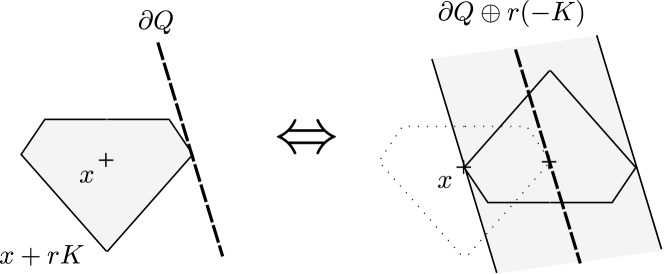
Figure 4: Relation between design centering and morphology

Now let us define domain estimation procedure $C(B,t)$ for box $B\in\mathcal{B}$ and threshold $t\in\mathbb{R}$ as follows:

$$C(B,t) =0\mbox{ if $B\cap Q=\emptyset$ or $B\subset\left(\partial Q\oplus t(-K)\right)$},$$ (7)

$$C(B,t) =1\mbox{ if $B\subset Q$ and $B\cap\left(\partial Q\oplus t(-K)\right)=\emptyset$},$$

$$C(B,t) =\beta\mbox{ in any other or unknown case}.$$

Notice that for star-shaped patterns $r_{1}(-K)\subset r_{2}(-K)$ whenever $r_{2}>r_{1}>0$. Combining this with (6) it can be easily seen that $C(B,t)$ is a domain estimation procedure for problem (5).

Intuitively our domain estimation procedure erodes the contour by the reflection of the pattern. The boxes lying too close to the contour boundary and not containing a good solution to the problem are marked empty. Eventually we shrink the search area to a small region containing the optimal solution. Formal study of this procedure is presented later in this section.

Let us continue with practical implementation of (7). In this section the main references are provided, see [48] for particular implementation details. Notice that the domain estimaiton procedure in the inverse graphical optimization algorithm is already defined on equally-sized boxes, so in fact we need volumetric images [18] of Minkowski sums and the contour. For the Minkowski sums we apply the general scheme based on convex decompositions [41]. First, we compute the convex decomposition of polyhedra and reduce the overall Minkowski sum to the union of pairwise convex ones. For the pattern decomposition we implement the surface flood-fill algorithm inspired by works [4, 10]; the contour boundary is used without any preprocessing as the set of simplex faces. Then we compute pairwise convex Minkowski sums with the help of CGAL [45]. After that we need to acqire the volumetric images of individual convex Minkowski sum. For this we involve a straightforward algorithm considering convex polytope as an intersection of half-spaces. As for the contour image, we first label the boundary boxes by a surface voxelization algorithms [33] and then separate inner and outer ones by testing a point inside every box. The latter is done with the help of simultaneous ray-casting procedure, which is essentially equivalent to a distance field computation along single direction [19].

Although some different techniques of Minkowski sums voxelization are known [20, 3], the method described above is rather easy to implement and fits perfectly into the inverse graphical method. The performance is good enough as well, see comparison at the end of the article.

The result domain estimation algorithm for threshold $t$ is as follows, refer to Fig. 5 and [48] for details.

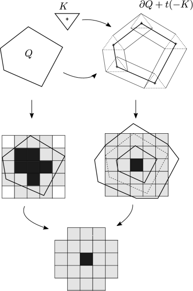
Figure 5: Domain estimation procedure for design centering

 

The domain estimation procedure for design centering

1. Decompose the contour boundary $\partial Q$ and the reflection of pattern $-K$ into convex parts.

2. Scale the reflected pattern convex parts by $t$.

3. Compute all the pairwise Minkowski sums of convex parts by the convex-hull based algorithm. We call these sums convex elements of $\partial Q\oplus t(-K)$.

4. Compute voxelizations of the convex elements on active boxes. This means that for every box under consideration in the inverse graphical algorithm we decide whenever it is inner, outer or boundary relative to the convex element.

5. Analogiously, we compute the voxelization of the contour itself.

6. Unite all the voxelizations. This is done by simple boolean operations on the results of previous steps for every box. By (7) we put $C(B,t)=0$ if $B$ is outside the contour at step 5 or $B$ is inside any element at step 4; $C(B,t)=1$ if $B$ is inside the contour at step 5 and $B$ is outside all the elements at step 4; $C(B,t)=\beta$ in all the remaining cases.

 

The theoretical result is given by the following theorem.

Theorem 6.

The domain estimation procedure defined by the algorithm above is problem-approximating.

See appendix section A for the proof.

Let us continue with constructing a convergent accuracy estimation procedure for the design centering problem under consideration. Although the general accuracy entimation procedure described in section 3.1 could be used, it is a bit complicated to prove its convergency. Nevertheless, it still gives a correct result by theorem 3 and even provided a better performance in practice, refer to section 4.3 for details. In this section we propose a simple method based on the Lipschitz property of the radius value to make a theoretically complete implementation. Precisely, the following theorem holds.

Theorem 7.

Consider a problem of form (5) and the inverse graphical optimization algorithm. Let $L$ be the Lipschitz constant of the radius value by theorem 5, $S$ be the domain scale and $\delta$ be the current accuracy in the algorithm. Then

$$\delta^{\prime}=(1+\frac{L}{S})\delta$$ (8)

is the convergent actual accuracy estimate.

For the proof refer to appendix section A. Note that the value of $L$ needed for (8) is easy to compute due to theorem 5. Now all the supporting algorithms required for the practical implementation of the inverse graphical optimization method for problem (5) are specified.

4.3 Comparison results

In this section we discuss the practical performance of the inverse and straight approaches to the diamond cutting problem described above. The algorithms have been implemented in C++ programming language and tested on various data using a machine with Core i7-8750H CPU and 16Gb RAM. For the implementation details refer to the source code published by the author [48]. We emphasize that only single-threaded CPU-based implementations have been tested as we aim on comparison of the general approaches. It is worth noting that one can apply more optimized algorithms mentioned above and in the references, especially parallelized and GPU-based ones. We leave these ideas for the future research.

The testing data used in comparison consists of publicly available diamond cut models [44] along with generated rough stone models of different resolution and complexity. Some examples are shown in Fig. 6 and Fig. 7. The precise data can be found at [48]. Note that we involve non-convex patterns as opposed to the traditional problem research. Besides, we have included some defects and irregularities in the rough stone models as they are common in the real-life industry

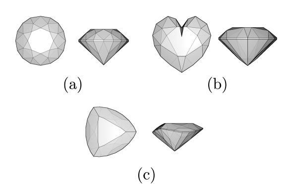
Figure 6: Diamond cut models: (a) standard_126, (b) rosehrttrue_104, (c) 1stwave_172

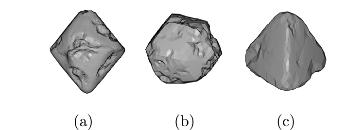
Figure 7: Rough stone models: (a) octa_rough_6432, (b) rhombic_rough_2304, (c) tetra_rough_912

Let us describe briefly the particular algorithms of global numerical optimization we compare. First, we have choosen a branch-and-bound variant due to Gourdin, Hansen and Jaumard, as it is stated to be the fastest in [15]. We denote it by ”GHJ” later in this section. Next, we consider modern Lipschitzian optimization schemes, not related to the branch-and-bound directly. The ones available in the open libraries are the DIRECT algorithm [17, 12] as provided by the nlopt library [47] and the LIPO scheme [22] implemented by the dlib C++ library [46]. Both algorithms are direct-search ones by nature. Recent research [22] indicates that their performance is competitive, however we were unable to reach meaningful results with LIPO. The reason seems to be in random sampling of the domain which takes too much time finding feasible points. Additionally, it is quite hard to implement a correct stopping criterion to get a proven optimal result. So we do not present this method in our research and refer the readers to [22] for a relative comparison with DIRECT and to [48] for the implementation and testing. As for DIRECT algorithm, the main problem is the absense of the proven precision estimations in nlopt library. So we have adapted the Lipschitzian bounds in the stopping criterion. For the comparisons we have choosen the best variants provided by the library, namely scaled DIRECT and locally-biased non-scaled DIRECT with randomization. We refer to them as ”DIRECT” and ”local DIRECT” respectively.

Concerning the inverse graphical method we include two variants in comparison differing only by the accuracy estimation procedure. As was described above, we implement the general scheme from section 3 as well as a Lipschitzian accuracy estimation procedure provided by theorem 7. We denote these variants as ”general inverse” and ”Lipschitzian inverse” respectively.

Let us proceed to the actual results. First, we compare the running times while searching for a proven global optimal solution with a specified precision. The results are presented in Table 1 with ”$>$ 5 hours” meaning that the algorithm failed to reach the target accuracy within five hours. As we can see, the inverse methods are superior, especially on hard problems and high precision requested. This remains true even when using the same Lipschitzian accuracy estimation as within the straight algorithms.

Problem	GHJ	DIRECT	local DIRECT	general inverse	Lipschitzian inverse
standard_126 rhombic_rough_576 1e-2	99	292	478	12	15
standard_126 rhombic_rough_576 1e-3	336	1665	2375	41	49
standard_126 rhombic_rough_576 1e-4	679	4663	6638	62	69
bstilltrue_194 rhombic_rough_2304 1e-2	$>$ 5 hours	$>$ 5 hours	$>$ 5 hours	193	638
rosehrttrue_104 tetra_rough_912 1e-2	5329	10347	$>$ 5 hours	69	78
rosehrttrue_104 tetra_rough_912 1e-3	11545	$>$ 5 hours	$>$ 5 hours	84	89
1stwave_172 tetra_flat_3648 1e-3	1568	$>$ 5 hours	$>$ 5 hours	160	165
novice7_86 octa_rough_6432 1e-2	1688	4526	5680	359	672
novice7_86 octa_rough_6432 1e-3	9434	$>$ 5 hours	$>$ 5 hours	1235	1268

Table 1: Runtimes acquiring proven solution, seconds

Next, we compare the time needed to accomplish the specified solution, see Table 2. Now we can see that DIRECT methods are reaching the good points earlier during computation. However, it is worth noting that in this case we need to know beforehand the optimal value we are actually looking for to stop the algorithm, otherwise we have no measure of the result quality.

Problem	GHJ	DIRECT	local DIRECT	general inverse	Lipschitzian inverse
standard_126 rhombic_rough_576 v1.429	97.18	7.70	3.44	37.40	37.54
bstilltrue_194 rhombic_rough_2304 v0.312	$>$ 5 hours	10.69	8.61	369.30	369.45
rosehrttrue_104 tetra_rough_912 v0.288	10147.29	14.43	24.57	94.52	95.04
1stwave_172 tetra_flat_3648 v5.089	1186.32	117.70	34.67	150.76	151.03
novice7_86 octa_rough_6432 v1.279	1587.34	87.43	84.09	1260.66	1247.45

Table 2: Runtimes reaching objective value, seconds

Combining all the results together we can conclude that the inverse graphical method is very promising for finding precise global optimal solutions to the optimization problems, and indeed provide ones within a practically tractable time. However, when one needs any good solution quickly regardless of its global quality, it is sensible to use something like DIRECT method or even local search.

In addition, note that one need to know the Lipschitz constant of the objective to get the proven global optimum by the straight methods. In contrast, the inverse scheme with general accuracy estimation does not depend on it to acquire the guaranteed result. Though it has not been proved theoretically that the algorithm would always finish in that case, in practice it does and even shows the best performance.

5 Conclusions and future work

A novel inverse approarch to deterministic global optimization has been developed within this article. It is based on domain estimation instead of objective value computation. We have proved theoretically its convergency and studied requirements on the procedures involved. The algorithm has been implemented in practice demonstrating clear advantage of the new method while searching for a proven global optimum for the design centering problem. Additionally, it have been shown that the inverse method is able to reach a guaranteed optimal solution even without knowing the Lipschitz constant, and the current theoretical results only depend on the continuity of the objective.

Concerning the application to the design centering, the problem has been extended to the case of non-convex star-shaped patterns and the complete implementation of various optimization methods has been provided.

Among drawbacks and future directions we should note that the inverse scheme depends heavily on estimation procedures and particular algorithms. These procedures differ in essence from the widely used black-box objective computations, and they could be hard or even impossible to implement for particular problems. So, it would be of high interest to research more applications of the inverse optimization approach, not necessarily the graphical one. Besides, it still remains to study sufficient conditions for the inverse graphical method to converge with the general accuracy estimation procedures. Nevertheless, the inverse technique is worth considering for the practical search of global solutions to optimization problems.

Appendix A Proofs

A.1 Supporting theory

First, let us prove some correctness lemmas for the inverse graphical optimization algorithm.

Lemma 2.

Consider the problem of form (2), any domain estimation procedure $C$ and any threshold $t\in\mathbb{R}$ satisfying

$$t>\min_{F}f(x).$$

Suppose box $B$ is empty under $C$ for threshold $t$; then for every threshold $t^{\prime}\leq t$ every box $B^{\prime}\subset B$ is empty as well.

Proof.

By the definition of the domain estimation procedure for every point $x\in B$ either $x\not\in F$ or $f(x)>t$. Consequently, for every point $x^{\prime}\in B^{\prime}\subset B$ either $x^{\prime}\not\in F$ or $f(x^{\prime})>t\geq t^{\prime}$. So, $B^{\prime}$ is empty by definition. ∎

Corollary 1.

Consider the inverse graphical optimization algorithm for the problem of form (2). Then the set of active boxes always covers the feasible set for the current threshold, i.e.

$$F(t)=\{x\in F\mid f(x)<t\}\subset\bigcup_{\mathcal{X}}X_{i}$$ (9)

at any step of the algorithm.

Proof.

At the beginning (9) holds obviously. After that $t$ is nonincreasing and we prune the empty boxes only, i.e. the ones containing no feasible points satisfying $f(x)<t$. It then follows from lemma 2 that (9) holds at any step of the algorithm. ∎

Now we continue with the proof that for every threshold satisfying $t>\min_{F}f(x)$ the boxes inside the feasible set eventually become filled by the inverse graphical algorithm. This property is crucial for the convergence of the algorithm iterations at steps 2 and 3c proved subsequently.

Lemma 3.

Consider the problem of form (2) and domain estimation procedure $C$. Suppose $C$ is problem approximating; then for every threshold $t$ satisfying

$$t>\min_{F}f(x)$$

there exists $\delta>0$ such that every cover of

$$F(t)=\{x\in F\mid f(x)<t\}\subset F$$

by boxes of size at most $\delta$ contains a filled box.

Proof.

Consider the objective function $f$ of the problem. By definition, $f$ is continuous and $F$ is compact with non-empty interior, so the problem solution

$$f_{min}=\min_{F}f(x)$$

is reached at some point. Assuming $f_{min}<t$ we additionally imply that $f(x)<t$ holds at least on some ball inside $F$ centered at $f_{min}$. Therefore, the set

$$I(t)=\{x\in\mathop{\mathrm{int}}\nolimits(F)\mid f(x)<t\}\subset F(t)$$

is nonempty. Consider any $x\in I(t)$ and $t$ as threshold. By definition 1 there exists $\delta>0$ such that every box $B$ of size $\delta(B)<\delta$ containing $x$ is filled. Every cover of $F(t)$ by boxes of size at most $\delta$ contains such a box, so the proof is completed. ∎

Corollary 2.

Consider the inverse graphical optimization algorithm for the problem of form (2). If the algorithm does not stop then

$$\delta\to 0.$$

In addition, suppose the domain estimation procedure is problem approximating. Then for every $\theta>0$ after finite number of steps in the algorithm

$$t<\min_{F}f(x)+\theta$$ (10)

if the algorithm does not stop before.

Proof.

First notice that step 2 of the algorithm finishes after finite number of iterations. Indeed, $t$ is decreased by a constant value $\delta$ and by lemma 1 it is strictly bounded from below by the problem solution. Consequently, if the algorithm does not stop at step 3 then it proceeds infinitely through step 5 and

$$\delta\to 0.$$

Now consider any $\theta>0$ and put

$$t^{\prime}=\min_{F}f(x)+\frac{\theta}{2}.$$

Suppose $t>t^{\prime}$, otherwise the corollary statement already holds. By corollary 1 the set of active boxes covers

$$F(t)=\{x\in F\mid f(x)<t\}$$

at every step of the algorithm. Obviously, $F(t^{\prime})\subset F(t)$, so the same boxes cover $F(t^{\prime})$. We proved above that box sizes

$$\delta(X_{i})=\frac{1}{S}\delta$$

eventually become as small as needed if the algorithm does not stop. It then follows from lemma 3 that there exists a filled box at some iteration of the algorithm for threshold $t^{\prime}$. Consequently, the iteration of step 2 continues at least until $t-\delta<t^{\prime}$ equivalent to $t<t^{\prime}+\delta$. This holds for any $\delta$ in the algorithm and $\delta\to 0$, so eventually

$$\delta<\frac{\theta}{2}$$

is satisfied. Combining the inequalities we obtain

$$t<t^{\prime}+\delta<\min_{F}f(x)+\frac{\theta}{2}+\frac{\theta}{2}=\min_{F}f(x)+\theta.$$

∎

Corollary 3.

Consider the inverse graphical optimization algorithm for the problem of form (2). Suppose the domain estimation procedure is problem approximating. Then step 3c of the algorithm finishes finding a filled box after finite number of attempts.

Proof.

After every attempt at step 3c we split all the boundary boxes reducing their sizes. By corollary 1 these boxes cover

$$F(t)=\{x\in F\mid f(x)<t\}.$$

Eventually box sizes become sufficiently small, so it then follows from lemma 3 that there exists a filled box and the iterating stops. ∎

A.2 Proof of theorem 2

Proof.

Consider target accuracy $\varepsilon>0$ and corresponding $\delta(\varepsilon)$, $\theta(\varepsilon)$ from definition 2. By corollary 2 after finite number of steps within the inverse graphical optimization algorithm we obtain

$$t<\min_{F}f(x)+\theta(\varepsilon)$$

and $\delta<\delta(\varepsilon)$ if the algorithm does not stop before. Hence, by definition 2 the convergent accuracy estimation procedure at step 3a of the algorithm produces

$$\delta^{\prime}<\varepsilon$$

after finite number of iterations. The algorithm then proceeds to step 3c which finishes in finite number of steps by corollary 3. So, the whole algorithm stops. ∎

A.3 Proof of theorem 3

Proof.

Indeed, the accuracy estimation procedure stops only when the result of domain estimation with threshold $t-\delta^{\prime}$ contains only empty boxes. This means by definition that for any $x\in F$

$$f(x)>t-\delta^{\prime}$$

or

$$\delta^{\prime}>t-f(x).$$

Note that $f(x)$ is continuous and $F$ is compact by the problem statement, so there exists $x_{min}$ such that

$$\min_{F}f(x)=f(x_{min}).$$

Combining with the previous inequality we obtain

$$\delta^{\prime}>t-f(x_{min})=t-\min_{F}f(x).$$

∎

A.4 Proof of theorem 4

Proof.

First statement of the theorem is straightforward. Indeed, the initial threshold search procedure returns $t$ only if the domain estimation procedure with threshold $t$ produces a filled box $B$. The latter means by definition that for any point $x\in B$ we have $x\in F$ and

$$t>f(x)\geq\min_{F}f(x).$$ (11)

Note that we start with non-empty box and only split boxes into $2^{n}$ equal parts, so $B\neq\emptyset$ and (11) actually holds.

Let us prove the second statement. Notice that the algorithm runs infinitely through step 4 if it does not stop. So, eventually

$$t>\min_{F}f(x)$$

becomes true and by problem definition there is a point $x\in F$ such that $t>f(x)$. After that the domain estimation procedure always produces a boundary or filled box by definition. This forces the initial threshold search procedure to either stop or run infinitely through step 6. In the latter case the boxes become arbitrarily small and the problem approximating domain estimation procedure eventually produce a filled box. The initial threshold search algorithm stops after that. ∎

A.5 Proof of theorem 5

Lemma 4.

Consider a star-shaped polytope $K$ having no faces coplanar with its origin $0$. Let $a\neq b$ be points in $\mathbb{R}^{n}$ such that rays $0a$, $0b$ intersect the same simplex face of $K$. Then for any point $x$ of the cut $[a,b]$ ray $0x$ intersects $\partial K$ at single point belonging to the same face.

Proof.

First notice that any ray starting at $0$ intersects $\partial K$ at single point. Indeed, any two points of intersection lie in the same face, otherwise one of them is not visible from $0$ violating star-shapeness condition. Thus, if there are two distinct intersection points then all the line passing through these points and containing $0$ is coplanar with the face, which is not allowed by the lemma statement.

Now denote by $D(y)$ the intersection point of ray $0y$ and $\partial K$. It remains to show that for any $x\in[a,b]$ $D(x)$ lies in face $F\subset\partial K$ whenever $D(a)\in F$ and $D(b)\in F$. In the rest of the proof we interpret all the points as vectors starting at $0$.

By lemma statement $0\not\in F$, so $D(a)\neq 0$, $D(b)\neq 0$, and by definition any $D(y)$ is collinear with $y$. Thus, there exist $s>0$, $k>0$ such that

$$D(a)=sa,\,D(b)=kb.$$

Moreover, $D(a)$, $D(b)$ lie in the same hyperplane containing face $F$, so there exist $n\in\mathbb{R}^{n}$, $c\in\mathbb{R}$ such that

$$D(a)\cdot n=c,\,D(b)\cdot n=c.$$

Combining equations we acquire

$$a\cdot n=\frac{c}{s},\,b\cdot n=\frac{c}{k}.$$

Now consider any $x\in[a,b]$. The latter means that there exists $\lambda\in[0,1]$ such that

$$x=\lambda a+(1-\lambda)b.$$

Let $D$ be the intersection point of line passing through $0$ and $x$ with hyperplane containing face $F$. This means that there exists $\mu\in\mathbb{R}\cup\infty$ such that

$$D=\mu x,\,D\cdot n=c.$$

Combining with previous equations we obtain

$$c=\mu x\cdot n=\mu\lambda a\cdot n+\mu(1-\lambda)b\cdot n=\mu\lambda\frac{c}{s}+\mu(1-\lambda)\frac{c}{k}.$$

Notice that by lemma statement $0$ is not coplanar with $F$, so $c\neq 0$. Therefore, from the previous equation

$$\mu=\frac{sk}{\lambda k+(1-\lambda)s}\in\mathbb{R}$$

Moreover, $s>0$ and $k>0$, so $\mu>0$, $\mu\neq\infty$ and $D=\mu x$ is the intersection of ray $0x$ and hyperplane of face $F$. We can express it as follows

$$D=\frac{sk}{\lambda k+(1-\lambda)s}\left(\lambda a+(1-\lambda)b\right)=\\ \frac{sk}{\lambda k+(1-\lambda)s}\left(\frac{\lambda}{s}D(a)+\frac{1-\lambda}{k}D(b)\right)=\\ \frac{\lambda k}{\lambda k+(1-\lambda)s}D(a)+\frac{(1-\lambda)s}{\lambda k+(1-\lambda)s}D(b).$$

From the latter we can see that $D$ is a convex combination of $D(a)$ and $D(b)$. Therefore, $D\in[D(a),D(b)]\subset F$, because by our convention all the faces are simplices. As was shown before, every ray starting at $0$ intersects $\partial K$ at single point, so $D(x)=D\in F$. ∎

Lemma 5.

Consider a star-shaped polytope $K$ having no faces coplanar with its origin $0$. Let $y_{1}$ and $y_{2}$ be points in $\mathbb{R}^{n}$ such that rays $0y_{1}$, $0y_{2}$ intersect the same simplex face $f$ of $K$. Suppose that $r_{1}>0$ and

$$y_{1}\in r_{1}K$$

then

$$y_{2}\in\left(r_{1}+L|y_{2}-y_{1}|\right)K$$

where

$$L=\frac{1}{\Delta}$$

and $\Delta$ is the minimum distance from origin $0$ to hyperplanes containing pattern faces.

Proof.

Let us put

$$r_{2}=r_{1}+L|y_{2}-y_{1}|$$

and consider scaled patterns $r_{1}K$ and $r_{2}K$. Notice that for any $r>0$ homothety with center $0$ and ratio $r$ transforms $K$ into $rK$ and lefts all the rays starting from $0$ in place. Therefore, for any $y\in\mathbb{R}^{n}$ and $r>0$ ray $0y$ intersects the boundary of $rK$ at image $rf$ of face $f$ whenever $0y$ intersects $\partial K$ at $f$. Let us denote by $D_{1}$, $D_{2}$ intersection points of rays $0y_{1}$, $0y_{2}$ with faces $r_{1}f$, $r_{2}f$ and by $H_{1}$, $H_{2}$ hyperplanes containing $r_{1}f$, $r_{2}f$ respectively, see Fig. 8.

Figure 8: Proof of lemma 5

Note that $D_{1}$ and $D_{2}$ are unique due to lemma 4. It then follows from lemma assumption $y_{1}\in r_{1}K$ and star-shapeness of $K$ that $|0y_{1}|\leq|0D_{1}|$, so $y_{1}$ and $0$ are in the same half-space bounded by $H_{1}$. In addition, notice that $r_{2}>r_{1}>0$, so it follows from the properties of homothety that $H_{2}$ is further from $0$ and parallel to $H_{1}$. Consequently, point $0$ and $H_{2}$ lie on the different sides of $H_{1}$. Combining with the above we deduce that $y_{1}$ and $H_{2}$ lie on the different sides of $H_{1}$ as well. Thus, the distance from $y_{1}$ to $H_{2}$ is greater than the distance between $H_{1}$ and $H_{2}$. Let us estimate the latter. Denote by $d$ the distance from $0$ to hyperplane containing $f$ in non-scaled pattern $K$. It then follows from the properties of homothety that the distance between parallel hyperplanes $H_{1}$ and $H_{2}$ is

$$d^{\prime}=(r_{2}-r_{1})d=Ld|y_{2}-y_{1}|.$$

By the lemma statement $L=\frac{1}{\Delta}$ and $\Delta\leq d$, therefore $Ld\geq 1$ and $d^{\prime}\geq|y_{2}-y_{1}|$. Notice that $|y_{2}-y_{1}|$ is precisely the distance between $y_{1}$ and $y_{2}$. Now remember that the distance between $y_{1}$ and $H_{2}$ is greater than $d^{\prime}$, therefore points $y_{1}$ and $y_{2}$, as well as $0$, lie in the same half-space bounded by $H_{2}$. Consequently,

$$|0y_{2}|\leq|0D_{2}|$$

by definition of $D_{2}$. It then follows from star-shapeness of $K$ that

$$y_{2}\in r_{2}K.$$

∎

of theorem 5.

Consider radius value at any point $x_{1}\in Q$:

$$r_{1}=r(x_{1})=\max\{r\geq 0\mid x_{1}+rK\subset Q\}$$

and let $x_{2}\in Q$ be any other point. Obviously, there exists a point $D\in(x_{1}+r_{1}K)\cap\partial Q$, otherwise $r_{1}$ can be increased a little bit keeping $x_{1}+r_{1}K\subset Q$. In the rest of the proof we treat all the points as vectors in $\mathbb{R}^{n}$ starting at $0$. For any point $y\in\mathbb{R}^{n}$ let us denote by $F(y)$ a single pattern face intersecting ray $0y$. Put

$$D_{1}=D-x_{1},\;D_{2}=D-x_{2}$$

and consider cut $\left[D_{1},D_{2}\right]$. From lemma 4 it follows that any set

$$\{y\in\left[D_{1},D_{2}\right]\mid F(y)=f\}$$ (12)

of points mapping to the same face $f$ is a continuous cut inside $\left[D_{1},D_{2}\right]$. By definition the pattern boundary consists of finite number of faces, so $\left[D_{1},D_{2}\right]$ is split into finite number of cuts of form (12), i.e.

$$\left[D_{1},D_{2}\right]=\bigcup_{i=1}^{n-1}\left[y_{i},y_{i+1}\right],$$

where the points of every cut $\left[y_{i},y_{i+1}\right]$ map to the same face under $F$. By definition $D\in x_{1}+r_{1}K$, so $D_{1}\in r_{1}K$. Applying lemma 5 to every pair of points $y_{i}$, $y_{i+1}$ starting with $D_{1}$ we obtain

$$D_{2}\in\left(r_{1}+\sum_{i=1}^{n-1}L|y_{i+1}-y_{i}|\right)K=\left(r_{1}+L|D_{2}-D_{1}|\right)K.$$

The latter combined with definitions of $D_{1}$ and $D_{2}$ leads to

$$D=x_{2}+D_{2}\in x_{2}+\left(r_{1}+L|x_{2}-x_{1}|\right)K.$$ (13)

Now put

$$r_{2}=r_{1}+L|x_{2}-x_{1}|$$

and consider any $r>r_{2}$. It then follows from (13) and star-shapeness of the pattern that

$$D\in x_{2}+r_{2}K\subset x_{2}+rK.$$ (14)

From lemma 4 we obtain that ray $x_{2}D$ intersects $\partial\left(rK\right)$ at single point $D^{\prime}$, and by the properties of homothety

$$D^{\prime}=x_{2}+\frac{r}{r_{2}}\left(D-x_{2}\right)\neq D.$$

Combining the latter with (14) we deduce that $D$ is an interior point of $x_{2}+rK$. By construction $D\in\partial Q$, therefore $x_{2}+rK\not\subset Q$ for any $r>r_{2}$. The latter immediately leads to

$$r(x_{2})\leq r_{2}=r_{1}+L|x_{2}-x_{1}|$$

which is the desired Lipschitz property. ∎

A.6 Proof of theorem 6

Proof.

First notice that all the filled boxes in the inverse graphical scheme are marked precisely by the algorithm of section 4.2. Indeed, by (6) at any step of the inverse graphical algorithm box $B$ is actually filled if and only if $B$ lies inside contour $Q$ and outside $\partial Q+t(-K)$. Moreover, Minkowski sum $\partial Q+t(-K)$ is the set union of convex elemets [41], so $B$ lies outside $\partial Q+t(-K)$ if and only if $B$ lies outside all the convex elements. So, every actually filled box does not intersect any geometry within the algorithm and is voxelized precisely as outer for every convex element and inner for the contour. This leads to precise marking at step 6 of the algorithm.

Now we trivially check definition 1 for the algorithm of this section. In scope of problem 2 suppose $x\in\mathop{\mathrm{int}}\nolimits(F)$ and $f(x)<t$. By the continuity of $f$ $f(x)<t$ holds in some neighbourhood $U(x)\subset F$. For sufficiently small $\delta$ any box $B$ with $\delta(B)<\delta$ containing $x$ lies inside $U$. By the definition such boxes are filled, so they are marked precisely, i.e. $C(B,t)=1$. ∎

A.7 Proof of theorem 7

Proof.

Note that (5) is a maximization problem, so all the relations of radius value and threshold through the proof will be in accordance to the problem and opposite to the study in section 3.

Now consider any $\varepsilon>0$ and let us specify values of $\delta(\varepsilon)$ and $\theta(\varepsilon)$ to satisfy definition 2. Indeed, by putting

$$\delta(\varepsilon)=\frac{S}{S+L}\varepsilon$$

we easily acquire

$$\delta^{\prime}<\left(1+\frac{L}{S}\right)\delta(\varepsilon)\leq\varepsilon$$

for the accuracy estimate $\delta^{\prime}$ whenever the curent accuracy satisfies $\delta<\delta(\varepsilon)$. The value of $\theta(\varepsilon)$ have no impact on the further study, so we just put $\theta(\varepsilon)=\varepsilon$. It then remains to make sure that $\delta^{\prime}$ is the actual accuracy estimate, i.e.

$$\delta^{\prime}\geq\max_{Q}r(x)-t$$

holds at every step 3a of the inverse graphical optimization algorithm. Indeed, the move from step 2 to step 3 in the optimization algorithm happens only when there are no boxes marked as filled by the domain estimation procedure for threshold $t+\delta$. In addition, it have been shown during the proof of theorem 6 that all the actually filled boxes are marked as filled. This means that every remaining active box $X_{i}\in\mathcal{X}$ is either outside the contour or contains a point $x_{i}$ within $\partial Q+(t+\delta)(-K)$ meaning that

$$r(x_{i})\leq t+\delta.$$

By theorem 5 for every $x\in X_{i}\cap Q$

$$r(x)-r(x_{i})\leq L\left|x-x_{i}\right|\leq L\delta(X_{i}),$$

where $\delta(X_{i})$ is the diameter of active box $X_{i}$. Therefore,

$$r(x)\leq t+\delta+L\delta(X_{i})$$

for every $x\in Q$ within active boxes. By step 5 of the algorithm $\delta=S\delta(X_{i})$, hence

$$r(x)\leq t+\delta+\frac{L}{S}\delta=t+\delta^{\prime}.$$ (15)

This holds for every feasible point in every active box. For all the prunned boxes $r(x)\leq t$ by step 2 of the algorithm. Therefore, (15) holds globally and

$$\max_{Q}r(x)\leq t+\delta^{\prime}$$

or equivalently

$$\delta^{\prime}\geq\max_{Q}r(x)-t.$$

This is exactly the definition of the actual accuracy estimate holding at every step 3a of the algorithm. ∎

References

- [1] Abaffy J., Galántai A.: An always convergent algorithm for global minimization of multivariable continuous functions. // Acta Polytechnica Hungarica, Vol. 15, Issue 1, pp. 177–195 (2018)
- [2] Aronov B., Sharir M.: On Translational Motion Planning of a Convex Polyhedron in 3-Space. // SIAM J. Comput., Vol. 26, Issue 6, pp. 1785–-1803 (1997)
- [3] Barki, H., Denis, F., Dupont, F.: Contributing vertices-based Minkowski sum of a non-convex polyhedron without fold and a convex polyhedron. // In: 2009 IEEE International Conference on Shape Modelling and Applications, pp. 73–80 (2009)
- [4] Chazelle, B., Dobkin, D., Shouraboura, N., Tal, A.: Strategies for polyhedral surface decomposition: An experimental study. // Comp. Geom. Theory Appl., Vol. 7, Issues 5-6, pp. 327–342 (1997)
- [5] Chebrolu, U., Kumar, P., Mitchell, J. S. B.: On Finding Large Empty Convex Bodies in 3D Scenes of Polygonal Models. // In: 2008 International Conference on Computational Sciences and Its Applications, pp. 382–393 (2008)
- [6] Contreras A. F. G., Ceberio M.: Comparison of strategies for solving global optimization problems using speculation and interval computations. // In: 2016 Annual Conference of the North American Fuzzy Information Processing Society (NAFIPS), pp. 1–6 (2016)
- [7] Deits, R., Tedrake, R.: Computing Large Convex Regions of Obstacle-Free Space Through Semidefinite Programming. // In: Algorithmic Foundations of Robotics XI: Selected Contributions of the Eleventh International Workshop on the Algorithmic Foundations of Robotics, pp. 109–124 (2015)
- [8] Solving Geometric Optimization Problems using Graphics Hardware. // Computer Graphics Forum, Vol. 22, Issue 3, pp. 441–451 (2003)
- [9] Dueck, G., Scheuer, T.: Threshold Accepting: A General Purpose Optimization Algorithm Superior to Simulated Annealing. // Journal of Computational Physics, Vol. 90, pp. 161–175 (1990)
- [10] Ehmann S., Lin M.: Accurate and fast proximity queries between polyhedra using convex surface decomposition. // Computer Graphics Forum, Vol. 20, Issue 3, pp. 500–511 (2001)
- [11] van Emden M.H.: Using the duality principle to improve lower bounds for the global minimum in nonconvex optimization. // In: Second COCOS workshop on intervals and optimization (2003)
- [12] Gablonsky J. M., Kelley C. T.: A Locally-Biased form of the DIRECT Algorithm. // Journal of Global Optimization, Vol. 21, Issue 1, pp. 27–37 (2001)
- [13] Hooker J. N.: Duality in optimization and Constraint Satisfaction. // In: International Conference on Integration of Artificial Intelligence (AI) and Operations Research (OR) Techniques in Constraint Programming, pp. 3–15 (2006)
- [14] Hooker J. N., van Hoeve W.-J.: Constraint programming and operations research. // Constraints, Vol. 23, Issue 2, pp. 172–195 (2017)
- [15] Horst, R., Pardalos, P.M.: Handbook of Global Optimization. Nonconvex Optimization and its Applications: Vol. 2. (1995)
- [16] Horst, R., Tuy, H.: Global Optimization: Determenistic Approaches. 3rd ed. (1996)
- [17] Jones D. R., Perttunen C. D., Stuckman B. E.: Lipschitzian optimization without the Lipschitz constant. // Journal of Optimization Theory and Applications, Vol. 79, Issue 1, pp. 157–181 (1993)
- [18] Kaufman, A.: Voxels as a Computational Representation of Geometry. // In: The Computational Representation of Geometry. SIGGRAPH ’94 Course Notes (1994)
- [19] Kobbelt, L., Botsch, M., Schwanecke, U., Seidel, H. P.: Feature-sensitive surface extraction from volume data. // In: Proc. of ACM SIGGRAPH, pp. 57–66 (2001)
- [20] Li, W., McMains, S.: Voxelized Minkowski Sum Computation on the GPU with Robust Culling. // Computer-Aided Design, Vol. 43, Issue 10, pp. 1270–1283 (2011)
- [21] Lien J.-M.: Hybrid motion planning using Minkowski sums. // In: Proc. Robotics: Science and Systems IV (2008)
- [22] Malherbe, C., Vayatis, N.: Global optimization of Lipschitz functions. arXiv:1703.02628 (2017)
- [23] Neumaier, A.: Complete search in continuous global optimization and constraint satisfaction. // Acta Numerica, Vol. 13, pp. 271–369 (2004)
- [24] Nguyen, V. H., Strodiot, J.-J.: Computing a global optimal solution to a design centering problem. // Mathematical Programing, Vol. 53, pp. 111–123 (1992)
- [25] Nocedal, J., Wright, S. J.: Numerical Optimization. (2006)
- [26] Lozano-Pérez T.: Spatial planning: A configuration space approach. // IEEE Trans. Comput., Vol. C-32, Issue 2, pp. 108–120 (1983)
- [27] Pustylnik, G: Spatial Planning with Constraints on Translational Distances between Geometric Objects. arXiv:0808.2931 (2008)
- [28] Rossi F., van Beek P., Walsh, T.: Handbook of Constraint Programming (Foundations of Artificial Intelligence). (2006)
- [29] Sacks, E., Kyung, M. H., Milenkovic, V.: Robust Minkowski Sum Computation on the GPU. // In: Computer Science Technical Reports, Paper 1765, Purdue University. (2013)
- [30] Sam-Haroud D.: Constraint consistency techniques for continuous domains. Ph.D. thesis, École polytechnique fédérale de Lausanne, Switzerland. (1995)
- [31] Sam-Haroud D., Faltings B.: Consistency techniques for continuous constraints. // Constraints, Vol. 1, Issue 1-2, pp. 85–118 (1996)
- [32] Scholz, D.: Determenistic Global Optimization: Geometric Branch-and-bound Methods and Their Applications. (2012)
- [33] Schwarz M.,Seidel H.-P.: Fast Parallel Surface and Solid Voxelization on GPUs. // ACM Transactions on Graphics, Vol. 29, Issue 6, Article No. 179. (2010)
- [34] Kvasov D. E., Sergeyev Ya. D.: Deterministic approaches for solving practical black-box global optimization problems. // Advances in Engineering Software, Vol. 80, pp. 58–66 (2015)
- [35] Serra J.: Image Analysis and Mathematical Morphology, Volume 1. (1982)
- [36] Shary S. P.: A Surprising Approach in Interval Global Optimization. // Reliable Computing, Vol. 7, Issue. 6, pp. 497–505 (2001)
- [37] Thoai N.: A Modified Version of Tuy’s Method for Solving d.c. Programming Problem. // Optimization: A Journal of Mathematical Programming and Operations Research, Vol. 19, Issue 5, pp. 665–674 (1988)
- [38] Thach P.: The Design Centering Problem as a D.C. Programming Problem. // Mathematical Programming, Vol. 41, pp. 229–248 (1988)
- [39] Thach, P., Tuy, H: The Relief Indicator Method for Constrained Global Optimization. // Naval Research Logistics, Vol. 37, pp. 473–497 (1990)
- [40] Tuy H.: Convex Analysis and Global Optimization. 2nd ed. (2016)
- [41] Varadhan, G., Manocha, D.: Accurate Minkowski Sum Approximation of Polyhedral Models. // Graphical Models, Vol. 68, Issue 4, pp. 343–355. (2006)
- [42] Winterfeld A.: Application of general semi-infinite programming to lapidary cutting problems. // European Journal of Operational Research, Vol. 191, Issue 3, pp. 838–854 (2008)
- [43] Wood G. R.: The bisection method in higher dimensions. // Mathematical Programming, Vol. 55, Issue 1-3, pp. 319–337 (1992)
- [44] http://3dlapidary.com
- [45] CGAL, Computational Geometry Algorithms Library. https://www.cgal.org
- [46] Dlib C++ Library http://dlib.net
- [47] Johnson S.G.: The NLopt nonlinear optmization package. http://ab-initio.mit.edu/nlopt
- [48] https://github.com/kserz/xdscribe