Axion boson stars

Abstract

We study novel solitonic solutions to Einstein-Klein-Gordon theory in the presence of a periodic scalar potential arising in models of axion-like particles. The potential depends on two parameters: the mass of the scalar field $m_{a}$ and the decay constant $f_{a}$; the standard case of the QCD axion is recovered when $m_{a}\propto 1/f_{a}$. When $f_{a}\to\infty$ the solutions reduce to the standard case of “mini” boson stars supported by a massive free scalar field. As the energy scale $f_{a}$ of the scalar self-interactions decreases we unveil several novel features of the solution: new stability branches emerge at high density, giving rise to very compact, radially stable, boson stars. Some of the most compact configurations acquire a photon sphere. When $f_{a}$ is at the GUT scale, a boson star made of QCD axions can have a mass up to ten solar masses and would be more compact than a neutron star. Gravitational-wave searches for these exotic compact objects might provide indirect evidence for ultralight axion-like particles in a region not excluded by the black-hole superradiant instability.

1 Introduction

The nature of dark matter remains one of the greatest mysteries in physics. The most compelling hypothesis is that dark matter is made of new particles beyond the Standard Model, but their properties mostly unknown. The mass of particle dark matter candidates spans a range of several tens of orders of magnitude (with candidates as light as $10^{-22}\,{\rm eV}$ or as massive as $10^{4}\,{\rm GeV}$). One of the most compelling dark-matter candidates is the axion [1, 2, 3], a pseudo Nambu-Goldstone boson which acquires a non-derivative coupling to the Standard Model only due to topological charges [4, 5, 6, 7, 8, 9]. While originally introduced by Peccei and Quinn to solve the strong CP problem in quantum chromodynamics (QCD), the axion later served as a prototype for weakly-interacting ultralight bosons beyond the Standard Model [10, 11, 12, 13]. For instance, axion-like particles (ALPs) with various masses are ubiquitous in string-theory compactification and have been suggested as a generic signature of extra dimensions [14, 15]. Several experiments are ongoing to search for ALPs in a wide mass range (for a recent review see Ref. [16]).

Ultralight bosons might form macroscopic Bose-Einstein condensates obtained as localized and coherently oscillating solutions to their classical field equations. When the boson mass is $\sim 10^{-22}\,{\rm eV}$, these condensates provide a natural alternative to the standard structure formation through dark matter seeds [17, 18, 19, 20, 21, 22]. When the boson mass is heavier, these condensates are smaller and can have the typical size and mass of an astrophysical compact object. These solutions are generically known as boson stars (BSs) (when the field is complex) or oscillatons [23] (when the field is real), and provide the prototypical example of an exotic compact object (ECO) [24], namely a hypothetical dark compact star that is neither a black hole nor a neutron star [25, 26].

More specifically, a BS (also known as Klein-Gordon geon) is a stationary configuration of a scalar field bounded by gravity [27, 28, 29, 23] (see Refs. [30, 31, 32, 33] for reviews), which is a solution to the Einstein-Klein-Gordon theory (see action (2.1) below). Both BSs and oscillatons can arise naturally as the end-state of gravitational collapse of scalar fields [23, 34, 35] and share similar features. If BSs can form in the universe, they might also form binary systems which would be a novel gravitational-wave (GW) source [36, 33, 24, 37, 38, 39]. The hypothetical detection of a BS could provide indirect evidence for physics beyond the Standard Model [40, 41].

The properties of BSs are strongly related to the scalar self-interactions of the model [27, 28, 29, 23, 42, 43, 44, 45]. For a given scalar potential, static BSs form a one-parameter family of solutions governed by the value of the bosonic field at the center of the star. Similarly to the case of perfect-fluid stars – whose properties depend on the value of the central density – the mass displays local maxima and minima corresponding to the threshold between branches of stability/instability against radial perturbations [46, 47, 48]. The maximum mass and compactness of a BS depend strongly on the boson self-interactions. As a rule of thumb, the stronger the self-interaction the higher the maximum compactness and mass of a stable BS [31, 32, 33, 45].

The scope of this work is to study a novel class of BSs obtained in the case of a periodic potential [cf. Eq. (2.12)] inspired by that of the QCD axion [1, 49]. The standard QCD axion model depends on a single parameter (either the axion mass or the axion decay constant, since these two quantities are inversely proportional to each other). We shall consider an extended version of the parameter space in which the scalar-field mass is independent from the decay constant, as in several ALP models [16]. Gravitationally bound configurations of QCD axions (dubbed axion stars) have been studied in the past few years [50, 51, 52, 53, 54, 55, 56, 57], mostly in the nonrelativistic limit or considering relativistic collisions in a limited number of configurations. One of our goals is to extend these studies to provide a detailed general relativistic description of equilibrium solutions and to include the case of an ALP potential in which the axion mass and the decay constant are independent from each other. Since we focus on complex scalar fields that oscillate in time, we shall dub our solutions as axion boson stars (ABSs). We refer to the Sec. 4 for a discussion about the close connection between complex- and real-field solutions.

2 Setup

2.1 Axion boson stars in Einstein-Klein-Gordon theory

BSs are equilibrium solutions to Einstein-Klein-Gordon theory

$$S=\int\text{d}^{4}x\sqrt{-g}\left[\frac{R}{2\kappa}-\tensor{g}{{}^{\alpha\beta}}\partial\indices{{}_{\alpha}}\psi\indices{{}^{*}}\partial\indices{{}_{\beta}}\psi-V(|\psi|^{2})\right]\ ,$$ (2.1)

where $\kappa=8\pi$, $R$ is the Ricci curvature, $\psi(x^{\mu})$ is a (generically complex) scalar field, and $V(|\psi|^{2})$ is the scalar self-interaction potential. The field equations are

$$\tensor{R}{{}_{\mu\nu}}-\frac{1}{2}\tensor{g}{{}_{\mu\nu}}R = \kappa\left(\partial\indices{{}_{\mu}}\psi\indices{{}^{*}}\partial\indices{{}_{\nu}}\psi+\partial\indices{{}_{\nu}}\psi\indices{{}^{*}}\partial\indices{{}_{\mu}}\psi-\tensor{g}{{}_{\mu\nu}}\left[\tensor{g}{{}^{\alpha\beta}}\partial\indices{{}_{\alpha}}\psi\indices{{}^{*}}\partial\indices{{}_{\beta}}\psi+V\right]\right)\,,$$ (2.2)

$$\dfrac{1}{\sqrt{-g}}\partial\indices{{}_{\alpha}}\left(\sqrt{-g}\,\tensor{g}{{}^{\alpha\beta}}\partial\indices{{}_{\beta}}\psi\right) = \dfrac{\partial\,V}{\partial|\psi|^{2}}\,\psi\,,$$ (2.3)

together with the complex conjugate of Eq. (2.3).

We consider spherically symmetric, equilibrium configurations, described by the line element

$$\text{d}s^{2}=-e^{v(r)}\text{d}t^{2}+e^{u(r)}\text{d}r^{2}+r^{2}\left[\text{d}\vartheta^{2}+\sin^{2}(\vartheta)\text{d}\varphi^{2}\right]\ ,$$ (2.4)

in terms of two real metric functions, $v(r)$ and $u(r)$. The scalar field is instead oscillating in time,

$$\psi=\phi(r)\,e^{i\omega t}\ .$$ (2.5)

where $\omega$ is a real parameter to be determined. The ansatz for the scalar field is required such that the equations of motion are real. With the above ansatz the field equations reduce to

$$\frac{1}{r^{2}}\,\frac{\partial}{\partial r}\left(r\,e^{-u}\right)-\frac{1}{r^{2}} = -\kappa\,\rho\ ,$$ (2.6)

$$e^{-u}\left[\frac{v^{\prime}}{r}+\frac{1}{r^{2}}\right]-\frac{1}{r^{2}} = \kappa p_{\rm rad}\ ,$$ (2.7)

$$\phi^{\prime\prime}+\left[\frac{2}{r}+\frac{v^{\prime}-u^{\prime}}{2}\right]\phi^{\prime} = e^{u}\left[U(\phi)-\omega^{2}e^{-v}\right]\ ,$$ (2.8)

where $U(\phi)=\text{d}V(\phi^{2})/\text{d}(\phi^{2})$ and we have introduced the energy density $\rho$ and the radial pressure $p_{\rm rad}$ which, together with the tangential pressure $p_{\rm tan}$, are expressed in terms of the stress-energy tensor of the scalar field, $T_{\alpha\beta}$, as follows

$$\rho \equiv -\tensor{T}{{}^{0}_{0}}=\omega^{2}e^{-v}\phi^{2}+e^{-u}{\phi^{\prime}}^{2}+V(\phi)\ ,$$ (2.9)

$$p_{\rm rad} \equiv \tensor{T}{{}^{1}_{1}}=\omega^{2}e^{-v}\phi^{2}+e^{-u}{\phi^{\prime}}^{2}-V(\phi)\ ,$$ (2.10)

$$p_{\rm tan} \equiv \tensor{T}{{}^{2}_{2}}=\omega^{2}e^{-v}\phi^{2}-e^{-u}{\phi^{\prime}}^{2}-V(\phi)\ .$$ (2.11)

Unlike the case of perfect fluid stars, the scalar field introduces anisotropies, $p_{\rm rad}\neq p_{\rm tan}$.

In the following we shall focus on a specific form of the potential, motivated by that of the QCD axion. The latter acquires a periodic potential due to non-linear instanton effects (for a detailed derivation, see Ref. [8]). We shall consider the following extension of the QCD axion potential:

$$V(\phi)=\frac{2\mu^{2}_{a}\,f_{a}^{2}}{\hbar B}\left(1-\sqrt{1-4\,B\,\sin^{2}\left(\dfrac{\phi\sqrt{\hbar}}{2\,f_{a}}\right)}\right)\ ,$$ (2.12)

where $B=\frac{z}{(1+z)^{2}}\approx 0.22$ and $z\equiv m_{u}/m_{d}\approx 0.48$ is the mass ratio of the up and down quarks. The second term in the above potential is the standard QCD axion potential [8], to which we added the first constant term to ensure $V(0)=0$ and hence asymptotically flat solutions.

In the above potential, $\mu_{a}$ and $f_{a}$ are two free parameters, with dimensions of an inverse length and of an energy, respectively. By expanding Eq. (2.12) around the minimum at $\phi=0$, we obtain

$$V(\phi)\sim\mu_{a}^{2}\phi^{2}-\left(\frac{3B-1}{12}\right)\frac{\hbar\mu_{a}^{2}}{f_{a}^{2}}\phi^{4}+{\cal O}(\phi^{6})\,,$$ (2.13)

from which we can identify the ALP mass

$$m_{a}=\mu_{a}\hbar\,,$$ (2.14)

and the ALP quartic coupling. In this model $\mu_{a}$ and $f_{a}$ are independent parameters. The case of a QCD axion is included when [8]

$$m_{a}\approx 5.7\,\mu{\rm eV}\left(\frac{10^{12}\,{\rm GeV}}{f_{a}}\right)\,.$$ (2.15)

Note that the expansion in Eq. (2.13) is valid when $f_{a}\gg\phi\sqrt{\hbar}$. In this limit, to the leading order, the potential reduces to the standard mass term, which leads to the family of so-called “mini” BSs [27, 28].

2.2 Numerical method

The field equations (2.6)-(2.8) can be solved for $v(r)$, $u(r)$ and $\phi(r)$ by imposing regularity boundary conditions at the center

$$\phi(0)=\phi_{c}\,,\quad u(0)=0\,,\quad v(0)=v_{c}\,,$$ (2.16)

and asymptotic flatness

$$\lim_{r\to\infty}\phi=0\,,\quad\lim_{r\to\infty}v=0\,.$$ (2.17)

The value of $v_{c}$ is arbitrary since it can be set to unity by a rescaling of the time coordinate.

For any choice of the central value of the scalar, $\phi_{c}$, the above conditions define a boundary value problem, whose eigenvalues $\omega=\omega_{m}$ form an infinite discrete set $(m=0,1,2,...$). We solve numerically the one-dimensional boundary-value problem through a shooting method [58, 59], following the same procedure detailed in Ref. [33]. For a given $\phi_{c}$, different eigenvalues correspond to the fundamental mode – for which the corresponding scalar eigenfunction has zero radial nodes ($m=0$) – and to excited states – with one ($m=1$) or more ($m>1$) nodes. Excited states are expected to be unstable and therefore we focus only on the fundamental mode [47].

As in the case of ordinary fluid stars, we can also characterize our solutions according to their total mass $M$ and radius $R$. Both quantities can be defined through the mass function ${\cal M}(r)$, given by

$${\cal M}(r)=\frac{r}{2}\left[1-e^{-u(r)}\right]\ .$$ (2.18)

Then, the total mass is $M={\cal M}(r\to\infty)$. At distances much larger than the Compton wavelength of the scalar field, the latter is exponentially suppressed but it has nonetheless support up to infinity. Therefore, there is no real vacuum for BS spacetimes. For this reason, the radius of a BS is not uniquely defined. It is customary to define an effective radius, $R$, as that containing $99\%$ of the mass, i.e., ${\cal M}(R)=0.99M$. Note that very compact BSs might have a very steep scalar profile, practically removing the ambiguity in the definition of the radius [33].

2.3 Stability analysis

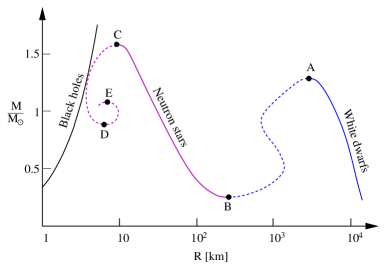
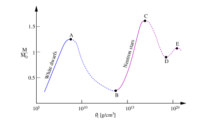
Figure 1: Schematic diagrams of the mass-radius (left) and mass-central density (right) relations for ordinary compact stars. The continuous (dotted) curves represent stable (unstable) equilibrium configurations. In the left diagram, the black curve represents the black-hole case, $R=2M$. Taken from Ref. [61] (adapted from [46]).

The radial stability analysis of a BS can be performed by looking at the $M(\phi_{c})$ and $M(R)$ diagrams, similarly to the case of perfect-fluid stars [46, 47, 48, 62]. A schematic representation of these diagrams for perfect-fluid stars is shown in Fig. 1. The critical points are those for which $dM/d\rho_{c}=0$ and correspond to a change of sign of a given radial mode, $w_{n}$. The stability can be studied by recalling that the modes are ordered, i.e. $w_{0}^{2}<w_{1}^{2}<w_{2}^{2}<...$, and that $dR/d\rho_{c}>0$ (resp. $dR/d\rho_{c}<0$) corresponds to the change of sign of a mode with odd (resp. even) value of $n$ [46].

Thus, if the left-most branch of the $M(\rho_{c})$ diagram is stable (“white dwarf” branch, $w_{n}^{2}>0$ for any $n$), the first point at which $dM/d\rho_{c}=0$ (Point A in Fig. 1) corresponds to $dR/d\rho_{c}<0$ and therefore $w_{0}^{2}$ changes sign, leading to an instability in the AB branch. In Point B $dR/d\rho_{c}<0$ so $w_{1}^{2}$ cannot change sign, nor can $w_{2}^{2}$ become negative since it must be larger than $w_{1}$. Therefore the only option is that $w_{0}^{2}$ returns positive, bringing back stability in the BC branch (“neutron star” branch). Following the same argument, it is straightforward to see that all configurations after Point C are unstable. This is due to the fact that $dR/d\rho_{c}$ is alternatively positive and negative at the extrema points D, E and so on, corresponding to the typical “curl” of the $M(R)$ diagram shown in Fig. 1. Therefore, standard perfect-fluid stars beyond the stable neutron-star branch are unstable and bound to either collapse to a black hole or to migrate to a stable stellar configuration by losing mass.

As we shall discuss, the same analysis can be performed for our ABS configurations, with the central scalar field $\phi_{c}$ playing the same role of the central mass density $\rho_{c}$ [47, 48]. In contrast with many BS models, ABSs can present many stable and unstable branches depending on the parameter $f_{a}$.

3 Results

Here we present the properties of spherically-symmetric ABSs by solving Eqs. (2.6)-(2.8) with the aforementioned boundary conditions and assuming the potential given in Eq. (2.12).

For the purpose of the numerical integration, it is convenient to use dimensionless quantities by performing the following rescaling

$$r\to\frac{\tilde{r}}{\mu_{a}}\ ;\quad{\cal M}(r)\to\frac{\tilde{{\cal M}}(\tilde{r})}{\mu_{a}}\ ;\quad\omega\to\tilde{\omega}\,\mu_{a}\ ;\quad\phi(r)\to\frac{\tilde{\phi}(\tilde{r})}{\sqrt{4\pi}}\ ;\quad f_{a}\to\tilde{f}_{a}\sqrt{\hbar}\ ,$$ (3.1)

where all tilded variables are dimensionless. (Henceforth we shall also rescale the radius and the mass as $\tilde{R}=R\mu_{s}$ and $\tilde{M}=R\mu_{s}$.) The rescaled field equations that we integrated numerically are given in Appendix A for completeness. Notice that the parameter $\mu_{a}$ disappears from the equations after the rescaling, so effectively any dimensionful quantity is written in units of $\mu_{a}$. This also implies that the mass and the radius of a given configuration scale as $1/\mu_{a}$ so they can assume any value depending on $\mu_{a}$. The compactness of the star, $M/R$, is instead independent of $\mu_{a}$ and therefore fixed for a given configuration.

Table 1: Representative examples of ABS configurations for $\tilde{f}_{a}=10$ (i.e., $f_{a}\approx 1.22\times 10^{20}\,\text{GeV}$). Configurations I and II correspond to that of maximum mass and that of maximum compactness. Since in this case $\tilde{f}_{a}\gg 1$, the results are in very good agreement with the mini BS case [36].

Configuration	$\tilde{\phi}_{c}$	$\tilde{\omega}$	$\tilde{M}$	$\tilde{R}$	$\tilde{R}/\tilde{M}$
I	$0.19150$	$0.85314$	$0.63299$	$7.86381$	$12.4231$
II	$0.43550$	$0.77018$	$0.51725$	$4.6588$	$9.00685$

As a check of our numerical method, we first integrate the equations for large values of $\tilde{f}_{a}$, which should reduce to the mini BS case. The large-$\tilde{f}_{a}$ limit is quickly saturated and $\tilde{f}_{a}\sim{\cal O}(10)$ is already in the asymptotic regime. In Table 1 we show two representative configurations for

$$\tilde{f}_{a}=10\quad\Rightarrow\quad f_{a}\approx 1.22\times 10^{20}\,\text{GeV}\ .$$ (3.2)

which are in very good agreement with the mini BS case [36], as expected. The above value of the decay constant corresponds to a mass of the QCD axion $m_{a}\approx 5.6\times 10^{-14}\,{\rm eV}$ [cf. Eq. (2.15)], which would give a maximum BS mass $M_{\rm max}\approx 1049\,M_{\odot}$ [cf. Table 1].

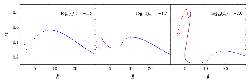
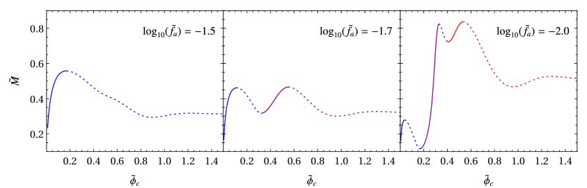
Figure 2: Mass-radius (upper panels) and mass-$\phi_{c}$ (lower panels) relation for ABSs for different values of $f_{a}$. Solid (dashed) curves correspond to stable (unstable) configurations. Different colors correspond to different branches. Decreasing the value of the energy scale $\tilde{f}_{a}$ causes the appearance of more stable/unstable branches.

In Fig. 2 we show the $M-R$ (upper panels) and $M-\tilde{\phi}_{c}$ (lower panels) diagrams for three representative cases. In the left panels we consider a relatively large value of $\tilde{f}_{a}$, which behaves similar to the mini BS limit. As expected the model displays a single stable branch up to a critical value of $\tilde{\phi}_{c}$, beyond which all configurations are unstable. Remarkably, the decrease of the decay constant leads to the formation of several new branches. As $\tilde{f}_{a}$ decreases, the $M-\tilde{\phi}_{c}$ diagram starts developing multiple maxima, which correspond to various turning points in the $M-R$ diagram, as shown Fig. 2. A radial stability analysis shows that new stable branches appear, which might correspond to very compact configurations. In the middle panels of Fig. 2 we show the case of $f_{a}\approx 2.4\times 10^{17}\,{\rm GeV}$, which leads to the formation of two stable branches, similarly to the fluid star case shown in Fig. 1, and also to the case of non-relativistic axion stars [51], and of solitonic BSs [33]. In the right panels of Fig. 2 we show the case $f_{a}\approx 1.2\times 10^{17}\,{\rm GeV}$, which leads to the formation of three stable branches. This is possible because – at variance with the previous case and with the perfect-fluid case shown in Fig. 1 – the second minimum of $M(\phi_{c})$ occurs when $dR/d\rho_{c}<0$, which in turn depends on the peculiar “turn” made by the second branch in the top-right panel of Fig. 2.

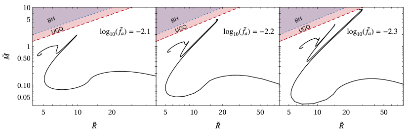
Figure 3: Same as in Fig. 2 but for a representative sample of ABSs with smaller values of $\tilde{f}_{a}$. Decreasing the value of $f_{a}$ leads to the appearance of more stable/unstable branches. Additionally, highly compact configurations, with $R\lesssim 3M$, also appear. The dotted and dashed straight line correspond to the black-hole case, $R=2M$, and to the photon-sphere radius, $R=3M$, which define the “ultracompact objects” (UCOs) introduced in Refs. [25, 26]. Even if $R>3M$ for all configurations, some of the most compact ones feature a photon-sphere and therefore classify as UCOs.

This peculiar behavior keeps occurring as $\tilde{f}_{a}$ decreases further. In this case the diagram becomes increasingly more intricate and highly sensitive to the value of $\tilde{f}_{a}$. This is shown in Fig. 3 for highly compact ABSs. As $\tilde{f}_{a}$ decreases, it becomes increasingly more difficult to find a solution, as the corresponding eigenvalue requires an extreme fine tuning. Thus, we were able to construct complete diagrams down at most to $\tilde{f}_{a}=10^{-2.3}$, corresponding to $f_{a}\approx 6\times 10^{16}\,{\rm GeV}$, i.e. close to the GUT scale.

As shown in Fig. 3, as $f_{a}$ decreases the most compact configurations approach the compactness $M/R\sim 1/3$. We expect that the compactness of such solutions increases when the value of $f_{a}$ decreases, i.e., that the curves in Fig. 3 approach more the UCO region [25, 26] (shaded region). Due to the numerical limitations of our code, we were unable to further explore the mass-radius diagram for smaller values of $f_{a}$. However, we performed a numerical search and we indeed confirm that the compactness decreases for smaller $f_{a}$, although always satisfying the bound $M/R>1/3$. Thus, the effective radius is always outside the Schwarzschild photon-sphere. However, since the radius of these solutions cannot be defined uniquely, we searched for light rings in our numerical solutions by computing the effective potential for null particles [63]. In regular, horizonless objects, due to the structure of the effective potential and to the centrifugal barrier at the center of the star, light-rings come in pair: an inner stable one and an outer unstable one [63, 64]. We found that a pair of light-rings appear for approximately $\log_{10}(\tilde{f}_{a})\leq-2.34$. Although it is numerically challenging to find ultracompact solutions with significantly smaller values of $f_{a}$, we expect that light-rings exist generically in this regime. Therefore, even if $R>3M$ for all configurations found in this work, the most compact ones – existing for $f_{a}\lesssim 6\times 10^{16}\,{\rm GeV}$ – classify as UCOs [25, 26].

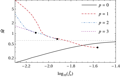
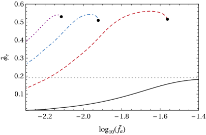
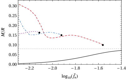
Figure 4: Mass (top-left), scalar field (top-right) and compactness (bottom) of the maximum mass MSCs as function of the axion decay constant. The dotted horizontal lines represent the mini BS limit and the markers indicate the appearance of additional branches at $\tilde{f}_{a}=\tilde{f}_{a}^{\rm crit}$. As $f_{a}$ decreases, more stable branches appear. The maximum mass of the first branch – the one with the BS limit (dotted line) – decreases as $f_{a}$ decreases, while the mass of the other branches increases. In the plots we track the first three additional branches, but subsequent branches appear for lower values of $\tilde{f}_{a}$ (three additional branches are shown in Table 2)

We notice that the appearance of additional branches continues for lower values of $f_{a}$. Each new branch corresponds to the appearance of two additional marginally stable configurations (MSCs) occurring at the maximum and minimum of the diagrams (see Fig. 2). In Fig. 4 we track the MSCs with maximum masses as function of $f_{a}$. We notice that while the mass of the first MSC – the one that has mini BS as limiting case – decreases as $f_{a}\to 0$, there are other MSCs whose masses increase quickly in the same limit. These solutions are responsible for the appearance of stable UCOs, discussed previously. Another interesting feature of these secondary MSCs is that they seem to appear around the same value of the central scalar field $\tilde{\phi}_{c}\sim 0.52$, and for critical values of the decay constant corresponding to the minima of the potential (where the latter also vanishes), i.e.

$$\tilde{f}_{a}^{\rm crit}\sim\frac{0.52}{4p\pi^{3/2}}\,,$$ (3.3)

with $p\geq 1$ being an integer label for the additional branches. In Table 2, we compare the numerical computation of $\tilde{f}_{a}^{\rm crit}$ with Eq. (3.3) for the first six additional branches. We see that the agreement improves for lower values of $f_{a}$. It is not clear up to which point this behavior (or the appearance of new branches) will hold for even lower values of $f_{a}$, but we expect this general trend of the solutions.

Table 2: Comparison between the numerically computed $\log_{10}(\tilde{f}_{a}^{\rm crit})$ and the analytical expression given by Eq. (3.3).

$p$	Numerical	Eq. (3.3)
1	-1.562	-1.6318
2	-1.922	-1.9328
3	-2.115	-2.1089
4	-2.242	-2.2338
5	-2.338	-2.3307
6	-2.416	-2.4099

4 Discussion

We were able to construct solutions with a decay constant as small as $f_{a}\approx 6\times 10^{16}\,{\rm GeV}$, i.e. close to the GUT scale. This corresponds to a QCD axion mass $m_{a}\approx 9.3\times 10^{-11}\,{\rm eV}$. It is worth noting that this value of the QCD axion mass evades the constraints coming from the black-hole superradiant instability [13, 65, 66, 67, 68, 69] for two reasons: first because the mass is slightly larger than what probed by superradiance (smaller values of $f_{a}$ would correspond to even larger masses, for which the superradiant constraints do not apply), and second because the corresponding value of the decay constant would give a relatively strong axion-photon coupling, potentially quenching the superradiant instability [70, 71].

In this unconstrained region of the parameter space [16], GW observations of isolated or binary ABSs might provide indirect evidence for ultralight bosonic fields in the universe. From the right top panel of Fig. 3, an axion with mass $m_{a}\approx 9.3\times 10^{-11}\,{\rm eV}$ and $f_{a}\approx 6\times 10^{16}\,{\rm GeV}$ would correspond to an ABS with maximum mass $M_{\rm max}\approx 9\,M_{\odot}$, and with a radius only slightly larger that of the photon-sphere, i.e. $M/R\lesssim 1/3$. The signal from the coalescence of such two ABSs would be very similar to that from two black holes with the same mass, but with some distinctive features [26]: (i) if the ABSs are spinning, their quadrupole moment would differ from that of a Kerr black hole [72]; (ii) even when the binary is nonspinning, tidal heating is expected to be negligible for BS binaries while it might affect a black-hole binary in a detectable way [73]; (iii) at variance with black holes, BSs can be tidally deformed in the last stages of the inspiral, similarly to neutron stars [39, 74]. These three effects would leave an imprint in the inspiral (at various post-Newtonian orders) compared to the case of a black-hole binary. Furthermore, the merger of two ABSs might be much richer than that of two black holes. For instance, scalar modes might be excited in the post-merger phase, and the merger remnant might be either a distorted ABS or a black hole, depending on the mass of the binary components [32, 37]. The mass-radius diagram in the right-top panel of Fig. 3 suggests that, when the decay constant is at the GUT scale, the merger of two ABSs with $M\approx 4\,M_{\odot}$ (corresponding to a compactness $M/R\approx 0.2$) can result in a radially stable ABS. The corresponding GW signal falls in the band of ground-based detectors. Furthermore, even for binaries with total mass exceeding the maximum mass of a given model, the presence of several stable branches makes it more difficult to predict the final state. Indeed, we expect multiple outcomes for the merger remnant, depending on the initial conditions. We therefore expect that inspiral-merger-ringdown consistency tests of the entire coalescence signal [75] can provide a strong discriminator between ABSs and black-hole binaries, similarly to case of two highly-compact “solitonic” BSs [37].

Furthermore, for an ALP field with $m_{a}\lesssim 10^{-16}\,{\rm eV}$, the corresponding ABS is supermassive, $M\gtrsim 10^{6}\,M_{\odot}$. While this is true for all BS models, in the ABS case when $f_{a}$ is sufficiently small the corresponding star is very compact and can feature a photon sphere. It would be therefore interesting to constrain this model with the recent shadow observation of the Event Horizon Telescope [76, 77]. In this case, isolated and binary supermassive ABSs would also be an exotic target of the LISA mission [78] and of evolved concepts thereof [79].

Although the most compact ABS configurations possess two light rings, our numerical results lead us to conjecture that the compactness of stable ABSs approaches the photon-sphere limit, $M/R=1/3$, but never exceeds it. This is possible because the geometry near the effective surface of the ABS is not Schwarzschild, and therefore a light ring might appear even when $R\gtrsim 3M$. It would be interesting to test our conjecture by decreasing the value of $\tilde{f}_{a}$ further and, possibly, to find an analytical explanation for the maximum value of the compactness of ABSs. Probing smaller values of $f_{a}$ is a natural technical extension of our work, which might be better achieved using relaxation methods [59], since the latter might be more efficient to find highly-compact solutions than the shooting method.

Another relevant follow-up of our work concerns the non-radial stability of ABSs, which requires a proper linear-perturbation analysis. In case such solutions turn out to be linearly stable, it would be interesting to study whether they can form in ABS collisions [54, 37, 57], or what would be the outcome of the coalescence of two highly-compact ABSs [54, 37].

For simplicity we focused on the case in which the scalar field is complex and oscillating in time. This gives a static stress-energy tensor and therefore a static metric, at variance with the case of oscillatons [23]. Both BSs and oscillatons can be formed as the end-state of gravitational collapse of scalar fields [23, 34, 35], and both configurations share similar features. Therefore, we expect that the properties discussed above for ABSs would be qualitatively the same also for axion stars made of a real field, which is the most relevant case for ALPs and the QCD axion.

Alternatively, due to the similarities of the solutions presented here with the solitonic BSs [80], it would be interesting to compare the general relativistic case with calculations in absence of gravity (i.e., considering Q-balls [81] or oscillons [82]). These solutions have been receiving considerable attention, and cases with oscillatory potentials similar to the one adopted here were explored recently [83, 84]. The existence of a Q-balls and oscillons with the same self-interacting potential could be an indication that these solutions might describe ultracompact objects when gravity is present.

Finally, BSs made of complex massive vector fields (so-called Proca stars) also exist and have properties similar to their scalar counterparts [43, 44]. We expect that Proca stars with a self-interaction potential similar to the one assumed in this work would share the same qualitative features of ABSs.

Appendix A Field equations in dimensionless form

For completeness we give here the field equations that we integrated numerically –after the rescaling (3.1). Setting $\tilde{r}=x$ and $W(x)=e^{v(x)}$, the final equations are

$$\begin{split}\tilde{{\cal M}}^{\prime}(x)-\frac{x}{B\,W(x)}\left[B\,W(x)\left(x-2\tilde{{\cal M}}(x)\right)\tilde{\phi}^{\prime}(x)^{2}+B\,x\,\omega^{2}\tilde{\phi}_{a}^{2}(x)\right.\\ \left.+8\pi\,x\,\tilde{f}_{a}^{2}\,W(x)\left(1-\sqrt{1-2\,B+2\,B\,\cos\left(\frac{\tilde{\phi}}{2\sqrt{\pi}\,\tilde{f}_{a}}\right)}\right)\right]=0\ ,\\ \end{split}$$ (A.1)

$$\begin{split}B\,x\left(x-2\,\tilde{{\cal M}}(x)\right)W^{\prime}(x)-\left[\left(2\,B\,x^{3}-4\,B\,x^{2}\,\tilde{{\cal M}}(x)\right)\tilde{\phi}^{\prime}(x)^{2}\right.\\ \left.-16\pi\,f_{a}^{2}\,x^{3}\left(1-\sqrt{1-2\,B+2\,B\,\cos\left(\frac{\phi(x)}{2\sqrt{\pi}\,f_{a}}\right)}\right)\right.\left.+2\,B\,\tilde{{\cal M}}(x)\right]W(x)-2\,B\,x^{3}\,\omega^{2}\,\tilde{\phi}(x)^{2}=0\ ,\\ \end{split}$$ (A.2)

$$\begin{split}\frac{x-2\,\tilde{{\cal M}}(x)}{x}\,\tilde{\phi}^{\prime\prime}(x)+\frac{2}{B\,x^{2}}\left[x\left(B-B\,\tilde{{\cal M}}(x)\right.\right.\\ \left.\left.-8\pi\,\tilde{f}_{a}^{2}\,x^{2}\left(1-\sqrt{1-2\,B+2\,B\,\cos\left(\frac{\tilde{\phi}(x)}{2\sqrt{\pi}\,f_{a}}\right)}\right)\right)\right]\tilde{\phi}^{\prime}(x)\\ +\frac{\omega^{2}}{W(x)}\,\tilde{\phi}(x)-\frac{2\sqrt{\pi}\,\tilde{f}_{a}}{\sqrt{1-2\,B+2\,B\,\cos\left(\frac{\tilde{\phi}(x)}{2\sqrt{\pi}\,f_{a}}\right)}}\,\sin\left(\frac{\tilde{\phi}(x)}{2\sqrt{\pi}\,f_{a}}\right)=0\ .\end{split}$$ (A.3)

References

- [1] Peccei, R. D. and Quinn, H. R., CP Conservation in the Presence of Instantons, Phys. Rev. Lett. 38 (1977) 1440–1443.
- [2] S. Weinberg, A new light boson?, Phys. Rev. Lett. 40 (Jan, 1978) 223–226.
- [3] F. Wilczek, Problem of strong and invariance in the presence of instantons, Phys. Rev. Lett. 40 (Jan, 1978) 279–282.
- [4] Preskill, J., Wise, M. B. and Wilczek, F., Cosmology of the Invisible Axion, Phys. Lett. 120B (1983) 127–132.
- [5] Davidson, S. and Schwetz, T., Rotating Drops of Axion Dark Matter, Phys. Rev. D93 (2016) 123509, [1603.04249].
- [6] Baer, H., Choi, K., Kim, J.E. and Roszkowski, L., Dark matter production in the early Universe: beyond the thermal WIMP paradigm, Phys. Rept. 555 (2015) 1–60, [1407.0017].
- [7] ADMX collaboration, Carosi, G., Searching for old (and new) light bosons with the axion dark matter experiment (ADMX), AIP Conf. Proc. 1441 (2012) 494–496.
- [8] Grilli di Cortona, G., Hardy, E., Pardo Vega, J. and Villadoro, G., The QCD axion, precisely, JHEP 01 (2016) 034, [1511.02867].
- [9] Klaer, Vincent B. and Moore, Guy D., The dark-matter axion mass, JCAP 1711 (2017) 049, [1708.07521].
- [10] J. Jaeckel and A. Ringwald, The Low-Energy Frontier of Particle Physics, Ann.Rev.Nucl.Part.Sci. 60 (2010) 405–437, [1002.0329].
- [11] R. Essig et al., Working Group Report: New Light Weakly Coupled Particles, in Community Summer Study 2013: Snowmass on the Mississippi (CSS2013) Minneapolis, MN, USA, July 29-August 6, 2013, 2013. 1311.0029.
- [12] M. Goodsell, J. Jaeckel, J. Redondo and A. Ringwald, Naturally Light Hidden Photons in LARGE Volume String Compactifications, JHEP 0911 (2009) 027, [0909.0515].
- [13] A. Arvanitaki and S. Dubovsky, Exploring the String Axiverse with Precision Black Hole Physics, Phys.Rev. D83 (2011) 044026, [1004.3558].
- [14] P. Svrcek and E. Witten, Axions In String Theory, JHEP 06 (2006) 051, [hep-th/0605206].
- [15] Arvanitaki, A., Dimopoulos, S., Dubovsky, S., Kaloper, N. and March-Russell, J., String Axiverse, Phys. Rev. D81 (2010) 123530, [0905.4720].
- [16] I. G. Irastorza and J. Redondo, New experimental approaches in the search for axion-like particles, Prog. Part. Nucl. Phys. 102 (2018) 89–159, [1801.08127].
- [17] Guzman, F. S. and Rueda-Becerril, J. M., Spherical boson stars as black hole mimickers, Phys. Rev. D80 (2009) 084023, [1009.1250].
- [18] A. Suárez, V. H. Robles and T. Matos, A Review on the Scalar Field/Bose-Einstein Condensate Dark Matter Model, Astrophys. Space Sci. Proc. 38 (2014) 107–142, [1302.0903].
- [19] B. Li, T. Rindler-Daller and P. R. Shapiro, Cosmological Constraints on Bose-Einstein-Condensed Scalar Field Dark Matter, Phys. Rev. D89 (2014) 083536, [1310.6061].
- [20] L. Hui, J. P. Ostriker, S. Tremaine and E. Witten, Ultralight scalars as cosmological dark matter, Phys. Rev. D95 (2017) 043541, [1610.08297].
- [21] P. S. B. Dev, M. Lindner and S. Ohmer, Gravitational waves as a new probe of Bose–Einstein condensate Dark Matter, Phys. Lett. B773 (2017) 219–224, [1609.03939].
- [22] P.-H. Chavanis, Collapse of a self-gravitating Bose-Einstein condensate with attractive self-interaction, Phys. Rev. D94 (2016) 083007, [1604.05904].
- [23] E. Seidel and W. Suen, Oscillating soliton stars, Phys.Rev.Lett. 66 (1991) 1659–1662.
- [24] G. F. Giudice, M. McCullough and A. Urbano, Hunting for Dark Particles with Gravitational Waves, JCAP 1610 (2016) 001, [1605.01209].
- [25] V. Cardoso and P. Pani, Tests for the existence of black holes through gravitational wave echoes, Nat. Astron. 1 (2017) 586–591, [1709.01525].
- [26] V. Cardoso and P. Pani, Testing the nature of dark compact objects: a status report, Living Rev. Rel. 22 (2019) 4, [1904.05363].
- [27] Kaup, D. J., Klein-Gordon Geon, Phys. Rev. 172 (1968) 1331–1342.
- [28] Ruffini, R. and Bonazzola, S., Systems of selfgravitating particles in general relativity and the concept of an equation of state, Phys. Rev. 187 (1969) 1767–1783.
- [29] M. Khlopov, B. A. Malomed and I. B. Zeldovich, Gravitational instability of scalar fields and formation of primordial black holes, Mon. Not. Roy. Astron. Soc. 215 (1985) 575–589.
- [30] P. Jetzer, Boson stars, Phys. Rept. 220 (1992) 163–227.
- [31] F. Schunck and E. Mielke, General relativistic boson stars, Class. Quant. Grav. 20 (2003) R301–R356, [0801.0307].
- [32] Liebling, S. L. and Palenzuela, C., Dynamical Boson Stars, Living Rev. Rel. 15 (2012) 6, [1202.5809].
- [33] Macedo, C. F. B., Pani, P., Cardoso, V. and Crispino, L. C. B., Astrophysical signatures of boson stars: quasinormal modes and inspiral resonances, Phys. Rev. D88 (2013) 064046, [1307.4812].
- [34] D. Garfinkle, R. B. Mann and C. Vuille, Critical collapse of a massive vector field, Phys. Rev. D68 (2003) 064015, [gr-qc/0305014].
- [35] H. Okawa, V. Cardoso and P. Pani, Collapse of self-interacting fields in asymptotically flat spacetimes: do self-interactions render Minkowski spacetime unstable?, Phys. Rev. D89 (2014) 041502, [1311.1235].
- [36] Macedo, Caio F. B., Pani, P., Cardoso, V. and Crispino, L. C. B., Into the lair: gravitational-wave signatures of dark matter, Astrophys. J. 774 (2013) 48, [1302.2646].
- [37] Palenzuela, C., Pani, P., Bezares, M., Cardoso, V., Lehner, L. and Liebling, S., Gravitational Wave Signatures of Highly Compact Boson Star Binaries, Phys. Rev. D96 (2017) 104058, [1710.09432].
- [38] Cardoso, V., Franzin, E. and Pani, P., Is the gravitational-wave ringdown a probe of the event horizon?, Phys. Rev. Lett. 116 (2016) 171101, [1602.07309].
- [39] V. Cardoso, E. Franzin, A. Maselli, P. Pani and G. Raposo, Testing strong-field gravity with tidal Love numbers, Phys. Rev. D95 (2017) 084014, [1701.01116].
- [40] L. Barack et al., Black holes, gravitational waves and fundamental physics: a roadmap, Class. Quant. Grav. 36 (2019) 143001, [1806.05195].
- [41] B. S. Sathyaprakash et al., Extreme Gravity and Fundamental Physics, 1903.09221.
- [42] A. H. Guth, M. P. Hertzberg and C. Prescod-Weinstein, Do Dark Matter Axions Form a Condensate with Long-Range Correlation?, Phys. Rev. D92 (2015) 103513, [1412.5930].
- [43] R. Brito, V. Cardoso, C. A. R. Herdeiro and E. Radu, Proca stars: Gravitating Bose-Einstein condensates of massive spin 1 particles, Phys. Lett. B752 (2016) 291–295, [1508.05395].
- [44] M. Minamitsuji, Vector boson star solutions with a quartic order self-interaction, Phys. Rev. D97 (2018) 104023, [1805.09867].
- [45] G. Choi, H.-J. He and E. D. Schiappacasse, Probing Dynamics of Boson Stars by Fast Radio Bursts and Gravitational Wave Detection, 1906.02094.
- [46] Shapiro, S. L. and Teukolsky, S. A., Black holes, white dwarfs, and neutron stars: The physics of compact objects. 1983, 10.1063/1.2915325.
- [47] T. D. Lee and Y. Pang, Stability of Mini - Boson Stars, Nucl. Phys. B315 (1989) 477.
- [48] M. Gleiser, Stability of Boson Stars, Phys. Rev. D38 (1988) 2376.
- [49] Peccei, R. D., QCD, strong CP and axions, J. Korean Phys. Soc. 29 (1996) S199–S208, [hep-ph/9606475].
- [50] Visinelli, Luca, Baum, Sebastian, Redondo, Javier, Freese, Katherine and Wilczek, Frank, Dilute and dense axion stars, Phys. Lett. B777 (2018) 64–72, [1710.08910].
- [51] Braaten, Eric, Mohapatra, Abhishek and Zhang, Hong, Dense Axion Stars, Phys. Rev. Lett. 117 (2016) 121801, [1512.00108].
- [52] Eby, Joshua, Leembruggen, Madelyn, Suranyi, Peter and Wijewardhana, L. C. R., QCD Axion Star Collapse with the Chiral Potential, JHEP 06 (2017) 014, [1702.05504].
- [53] Eby, Joshua, Leembruggen, Madelyn, Suranyi, Peter and Wijewardhana, L. C. R., Collapse of Axion Stars, JHEP 12 (2016) 066, [1608.06911].
- [54] T. Helfer, D. J. E. Marsh, K. Clough, M. Fairbairn, E. A. Lim and R. Becerril, Black hole formation from axion stars, JCAP 1703 (2017) 055, [1609.04724].
- [55] E. D. Schiappacasse and M. P. Hertzberg, Analysis of Dark Matter Axion Clumps with Spherical Symmetry, JCAP 1801 (2018) 037, [1710.04729].
- [56] P.-H. Chavanis, Phase transitions between dilute and dense axion stars, Phys. Rev. D98 (2018) 023009, [1710.06268].
- [57] K. Clough, T. Dietrich and J. C. Niemeyer, Axion star collisions with black holes and neutron stars in full 3D numerical relativity, Phys. Rev. D98 (2018) 083020, [1808.04668].
- [58] M., Douglas, B., Silvana and E.W., Ralph, The shooting technique for the solution of two-point boundary value problems, Maple Tech 3 (11, 1995) .
- [59] Press, William H., Teukolsky, Saul A., Vetterling, William T. and Flannery, Brian P., Numerical Recipes in FORTRAN: The Art of Scientific Computing, .
- [60] B. Hartmann, B. Kleihaus, J. Kunz and I. Schaffer, Compact Boson Stars, Phys. Lett. B714 (2012) 120–126, [1205.0899].
- [61] B. Kleihaus, J. Kunz and S. Schneider, Stable Phases of Boson Stars, Phys. Rev. D 85 (2012) 024045, [1109.5858].
- [62] P.-H. Chavanis, Mass-radius relation of newtonian self-gravitating bose-einstein condensates with short-range interactions. i. analytical results, Phys. Rev. D 84 (Aug, 2011) 043531.
- [63] V. Cardoso, L. C. B. Crispino, C. F. B. Macedo, H. Okawa and P. Pani, Light rings as observational evidence for event horizons: long-lived modes, ergoregions and nonlinear instabilities of ultracompact objects, Phys. Rev. D90 (2014) 044069, [1406.5510].
- [64] P. V. P. Cunha, E. Berti and C. A. R. Herdeiro, Light-Ring Stability for Ultracompact Objects, Phys. Rev. Lett. 119 (2017) 251102, [1708.04211].
- [65] A. Arvanitaki, M. Baryakhtar and X. Huang, Discovering the QCD Axion with Black Holes and Gravitational Waves, Phys. Rev. D91 (2015) 084011, [1411.2263].
- [66] R. Brito, V. Cardoso and P. Pani, Superradiance, Lect. Notes Phys. 906 (2015) pp.1–237, [1501.06570].
- [67] R. Brito, S. Ghosh, E. Barausse, E. Berti, V. Cardoso, I. Dvorkin et al., Stochastic and resolvable gravitational waves from ultralight bosons, Phys. Rev. Lett. 119 (2017) 131101, [1706.05097].
- [68] R. Brito, S. Ghosh, E. Barausse, E. Berti, V. Cardoso, I. Dvorkin et al., Gravitational wave searches for ultralight bosons with LIGO and LISA, Phys. Rev. D96 (2017) 064050, [1706.06311].
- [69] V. Cardoso, O. J. C. Dias, G. S. Hartnett, M. Middleton, P. Pani and J. E. Santos, Constraining the mass of dark photons and axion-like particles through black-hole superradiance, JCAP 1803 (2018) 043, [1801.01420].
- [70] T. Ikeda, R. Brito and V. Cardoso, Blasts of Light from Axions, Phys. Rev. Lett. 122 (2019) 081101, [1811.04950].
- [71] M. Boskovic, R. Brito, V. Cardoso, T. Ikeda and H. Witek, Axionic instabilities and new black hole solutions, Phys. Rev. D99 (2019) 035006, [1811.04945].
- [72] N. V. Krishnendu, K. G. Arun and C. K. Mishra, Testing the binary black hole nature of a compact binary coalescence, Phys. Rev. Lett. 119 (2017) 091101, [1701.06318].
- [73] A. Maselli, P. Pani, V. Cardoso, T. Abdelsalhin, L. Gualtieri and V. Ferrari, Probing Planckian corrections at the horizon scale with LISA binaries, Phys. Rev. Lett. 120 (2018) 081101, [1703.10612].
- [74] Sennett, N., Hinderer, T., Steinhoff, J., Buonanno, A. and Ossokine, S., Distinguishing Boson Stars from Black Holes and Neutron Stars from Tidal Interactions in Inspiraling Binary Systems, Phys. Rev. D96 (2017) 024002, [1704.08651].
- [75] Virgo, LIGO Scientific collaboration, Abbott, B. P. et al., Tests of general relativity with GW150914, Phys. Rev. Lett. 116 (2016) 221101, [1602.03841].
- [76] Event Horizon Telescope collaboration, K. Akiyama et al., First M87 Event Horizon Telescope Results. I. The Shadow of the Supermassive Black Hole, Astrophys. J. 875 (2019) L1.
- [77] H. Olivares, Z. Younsi, C. M. Fromm, M. De Laurentis, O. Porth, Y. Mizuno et al., How to tell an accreting boson star from a black hole, 1809.08682.
- [78] H. Audley, S. Babak, J. Baker, E. Barausse, P. Bender, E. Berti et al., Laser Interferometer Space Antenna, ArXiv e-prints (Feb., 2017) , [1702.00786].
- [79] V. Baibhav et al., Probing the Nature of Black Holes: Deep in the mHz Gravitational-Wave Sky, 1908.11390.
- [80] T. D. Lee and Y. Pang, Nontopological solitons, Phys. Rept. 221 (1992) 251–350.
- [81] S. R. Coleman, Q Balls, Nucl. Phys. B262 (1985) 263.
- [82] I. L. Bogolyubsky and V. G. Makhankov, On the Pulsed Soliton Lifetime in Two Classical Relativistic Theory Models, JETP Lett. 24 (1976) 12.
- [83] K. Mukaida, M. Takimoto and M. Yamada, On Longevity of I-ball/Oscillon, JHEP 03 (2017) 122, [1612.07750].
- [84] J. Eby, K. Mukaida, M. Takimoto, L. C. R. Wijewardhana and M. Yamada, Classical nonrelativistic effective field theory and the role of gravitational interactions, Phys. Rev. D99 (2019) 123503, [1807.09795].